Periodic orbits in Rössler system

Abstract.

We prove the existence of $n$-periodic orbits for almost all $n\in\mathbb{N}$ in the Rössler system with attracting periodic orbit, for two sets of parameters. The proofs are computer-assisted.

1. Introduction

Rössler in [13] studied the system

(1) $$\begin{cases}x^{\prime}=-y-z,\\ y^{\prime}=by+x,\\ z^{\prime}=z(x-a)+b\end{cases}$$

with $a=5.7$, $b=0.2$ as an example of a low-dimensional polynomial system with a single nonlinear term, which admits chaotic behaviour. The existence of symbolic dynamics in it was proven with computer assistance in [17]. Studying Rössler system’s dynamics and its periodic orbits for varying parameters is an active field of research (see [7, 9, 16, 2, 12, 4] and references therein).

Numerical simulations of the Rössler system show that for wide range of parameters for suitable Poincaré map there exists an attracting set, which is essentially one dimensional. In such a situation one expects that the forcing relations between periods described in the Sharkovskii’s theorem should be applicable. Let us recall the Sharkovskii’s theorem in its original form in dimension one (see [14, 15, 1]):

Theorem 1 (Sharkovskii).

Define an ordering ‘$\triangleleft$’ of natural numbers:

$$\begin{array}[]{r@{\ \triangleleft\ }c@{\ \triangleleft\ }c@{\ \triangleleft\ }c@{\ \triangleleft\ }l}3\triangleleft 5\triangleleft 7\triangleleft 9\triangleleft\dots&2\cdot 3&2\cdot 5&2\cdot 7&\dots\\ \dots&2\cdot 3^{2}&2\cdot 5^{2}&2\cdot 7^{2}&\dots\\ \dots&2\cdot 3^{3}&2\cdot 5^{3}&2\cdot 7^{3}&\dots\\ \lx@intercol\hfil\dots\dots\dots\dots\dots\dots\dots\dots\dots\dots\hfil\lx@intercol\\ \dots&2^{k+1}&2^{k}&2^{k-1}&\ldots\ \triangleleft 2^{2}\triangleleft 2\triangleleft 1.\\ \end{array}$$

Let $f:I\to\mathbb{R}$ be a continuous map of an interval. If $f$ has an $m$-periodic point and $m\triangleleft n$, then $f$ also has an $n$-periodic point.

In [20, 19] the above theorem has been extended to multidimensional perturbations of 1-dimensional maps and in [18] it is explained how it fits to the symbolic dynamics established [17] for system (1) with $a=5.7$, $b=0.2$.

In our study of (1) we fix $b=0.2$. Consider the Poincaré map $P$ partly defined on the section $\Pi=\{x=0,y<0\}$. Studying the bifurcation diagram for $(a,y)$ (see Fig. 1) we see that a $3$-periodic attracting orbit appears, for example, for $a=5.25$. The other interesting case is the $5$-periodic attracting point for $a=4.7$. These are two sets of parameter values treated in our work.

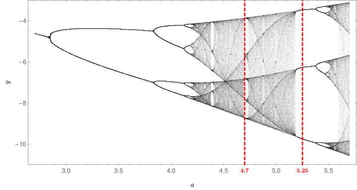
Figure 1. Bifurcation diagram for the Poincaré map of the system (1) with $b=0.2$. The attracting periodic orbits for $a=4.7$ and $a=5.25$ are expected ($3$-periodic for $a=5.25$ and $5$-periodic for $a=4.7$, respectively).

From numerical evidence we see that $P$ exhibits a strong contraction in the $z$ direction and the invariant sets containing the periodic orbits are almost 1-dimensional (see Figs. 5 and 10). Therefore we can assume in both cases considered in our work (and, most probably, also for a larger range of $a$s) that $P$ can be treated as a 2-dimensional perturbation of a 1-dimensional model map. Hence, as suggested by Theorem 1 and its multidimensional version from [20, 19, 18], we can expect a large set of periodic points also for $P$.

In this paper we prove the existence of all periods for $a=5.25$ (with an attracting $3$-periodic orbit). In the second case, $a=4.7$ (with an attracting orbit of period $5$), we show the existence of all periods with an exception of the period $3$, which agrees with the forcing relation between periods for interval maps described in Theorem 1. Moreover, we show that the period $3$ is indeed not realised in an attracting set for $P$.

The methods used in the present work combine the topological tools, the covering relations, with rigorous numerics. Our proofs are inspired by the approach to multidimensional perturbations of 1-dimensional maps from [20, 19, 18], but the strategy of constructing suitable covering relations needed to obtain the desired infinite sets of periodic orbits is different. In the second case some orbits with low periods has been established using the interval Newton method [11].

All the programs are written in C++ with the use of CAPD (Computer-Assisted Proofs in Dynamics) library [3, 8] for interval arithmetic, differentiation and integration.

2. Notation

In the paper, we consider the system (1) with fixed $b=0.2$ and $a=5.25$ or $a=4.7$. In both cases, we denote by $\Pi$ the half-plane $\{x=0,y<0\}$ with induced coordinates $(y,z)$, and $P$ is a Poincaré map on section $\Pi$, that is the map

$$P(y,z)=\pi_{(y,z)}\left(\Phi_{T(y,z)}\left(x=0,y,z\right)\right)\text{,}$$

where $\pi_{(y,z)}$ is the projection on the $(y,z)$ plane, $\Phi_{t}$ is the dynamical system induced by considered system and $T=T(y,z)$ is a return time, if well-defined. Note that for $y+z=0$ the vector field given by the right-hand-side of (1) is not transversal to $\Pi$. In our area of interest, however, $z$ is sufficiently small to guarantee $\dot{x}>0$ on the section.

To simplify the notation, by ‘$n$-periodic orbit’ or ‘point’, we understand an orbit or point with basic period $n$ for map $P$. Whenever we refer to a ‘$n$-periodic orbit of the system’ we mean a periodic orbit of the system, which passes through an $n$-periodic orbit of $P$.

3. Horizontal covering and periodic points

The idea of one-dimensional covering relation between intervals which Block et al. [1] used to prove Sharkovskii’s theorem (Th. 1) is given by the following definition.

Definition 1.

Assume that $I,J\subset\mathbb{R}$ are intervals and $f:I\to\mathbb{R}$ is continuous.

An interval $I$ $f$-covers $J$ (denoted by $I\overset{f}{\longrightarrow}J$) if there exists a subinterval $K\subset I$ such that $f(K)=J$.

The following easy theorem gives the periodic orbits in the proofs of Sharkovskii’s theorem (see, for example, [1]).

Theorem 2.

Assume that $f:\mathbb{R}\supset I\to\mathbb{R}$ is continuous and we have a sequence of intervals $I_{j}\subset I$ for $j=0,\dots,n-1$ such that

$$I_{0}\overset{f}{\longrightarrow}I_{1}\overset{f}{\longrightarrow}I_{2}\overset{f}{\longrightarrow}\dots\overset{f}{\longrightarrow}I_{n-1}\overset{f}{\longrightarrow}I_{0}.$$

Then there exists $x\in I_{0}$, such that $f^{j}(x)\in I_{j}$ for $j=1,\dots,n-1$ and $f^{n}(x)=x$.

For higher-dimensional perturbations of $f$ a stronger notion of covering is needed to have an analogous result. We use the notion of the horizontal covering from [20, 18] with small modifications. It is simplified, set in two-dimensional space, and the notion of ‘left-’ and ‘right side’ is slightly extended.

By $\mathcal{C}(r)$ we will denote the family of rectangles (two-dimensional cylinders) of the form $[a,b]\times[-r,r]\subset\mathbb{R}^{2}$ for $r>0$.

Definition 2.

A two-dimensional h-set (shortly: an h-set) is a rectangle $N=[a,b]\times[-r,r]\in\mathcal{C}(r)$ with the following elements distinguished:

• its left edge  $L(N)=\{a\}\times[-r,r]$;

• its right edge  $R(N)=\{b\}\times[-r,r]$;

• its horizontal boundary  $H(N)=[a,b]\times\{-r,r\}$;

• its left side  $S_{L}(N)=(-\infty,a)\times(-\infty,\infty)$;

• its right side  $S_{R}(N)=(b,\infty)\times(-\infty,\infty)$.

We need these notions to define horizontal covering relation.

Definition 3.

Let $N_{0}$, $N_{1}\in\mathcal{C}(r)$ be two h-sets and $f:\mathbb{R}^{2}\to\mathbb{R}^{2}$. We say that $N_{0}$ $f$-covers $N_{1}$ horizontally and denote by $N_{0}\overset{f}{\Longrightarrow}N_{1}$ if

(2) $$f(N_{0})\subset S_{L}(N_{1})\cup N_{1}\cup S_{R}(N_{1})\setminus H(N_{1})\text{,}$$

and one of the two conditions hold:

(3) either $$f(L(N_{0}))\subset S_{L}(N_{1}) \text{\quad and \quad}f(R(N_{0}))\subset S_{R}(N_{1})\text{,}$$

or $$f(L(N_{0}))\subset S_{R}(N_{1}) \text{\quad and \quad}f(R(N_{0}))\subset S_{L}(N_{1}).$$

See Fig. 2 for the illustration of horizontal covering.

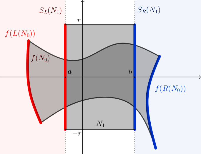
Figure 2. Horizontal covering $N_{0}\overset{f}{\Longrightarrow}N_{1}$

Let us emphasize that the above conditions can be easily checked with the use of computer via interval arithmetic and ‘$<$’, ‘$>$’ relations.

The following theorem might be seen as the generalization of Theorem 2.

Theorem 3 ([20]).

Suppose that we have a loop of $n$ horizontal $f$-coverings:

$$N_{0}\overset{f}{\Longrightarrow}N_{1}\overset{f}{\Longrightarrow}\dots\overset{f}{\Longrightarrow}N_{n-1}\overset{f}{\Longrightarrow}N_{n}=N_{0}\text{,}$$

then there exists $x\in\operatorname{int}N_{0}$ such that $f^{n}(x)=x$ and

$$\text{for }i=0,\dots,n-1:\qquad f^{i}(x)\in\operatorname{int}N_{i}.$$

The example of topological horseshoe discussed below shows how from a finite number of covering relations we can obtain periodic orbits of all periods.

Example 1 (A topological horseshoe).

Let $N_{0}$, $N_{1}\subset\mathcal{C}(r)$ be two disjoint h-sets. Suppose that a continuous map $f:\mathbb{R}^{2}\to\mathbb{R}^{2}$ fulfils the horizontal covering relations (see Fig. 3)

(4) $$\begin{array}[]{cc}N_{0}\overset{f}{\Longrightarrow}N_{0}\text{,}&N_{0}\overset{f}{\Longrightarrow}N_{1}\text{,}\\ N_{1}\overset{f}{\Longrightarrow}N_{0}\text{,}&N_{1}\overset{f}{\Longrightarrow}N_{1}.\end{array}$$

Figure 3. Topological horseshoe in $\mathbb{R}^{2}$: each $N_{0,1}$ covers itself and the other set. The vertical egdes of $N_{0}$ and $N_{1}$ are marked in red and green, respectively.

Such a map is called in literature a topological horseshoe for $N_{0}$, $N_{1}$ [10].

Choose now any finite sequence of zeros and ones of any length $l$ : $(i_{0},i_{1},\dots,i_{l-1})$, $i_{k}\in\{0,1\}$. The conditions (4) imply in particular the following chain of covering relations:

$$N_{i_{0}}\overset{f}{\Longrightarrow}N_{i_{1}}\overset{f}{\Longrightarrow}\dots\overset{f}{\Longrightarrow}N_{i_{l-1}}\overset{f}{\Longrightarrow}N_{i_{0}}\text{,}$$

and, from Theorem 3, we can deduce that there exists an $l$-periodic orbit for $f$, which additionally moves between the sets $N_{0}$, $N_{1}$ according to the pattern $(i_{0},i_{1},\dots,i_{l-1})$. We can do it for any period $l$ and we are able to choose such a sequence of length $l$ to be sure that $l$ is the fundamental period of the orbit.

The same is also true for (bi-)infinite sequences of indicators $i_{k}$. In general, the maps admitting a topological horseshoe are semi-conjugate to the dynamical system generated on the space $\Sigma_{2}=\{0,1\}^{\mathbb{Z}}$ by the shift map, called also the symbolic dynamics [10].

4. Orbits of all periods for $a=5.25$

Consider now the system (1) with $a=5.25$, $b=0.2$, that is

(5) $$\begin{cases}x^{\prime}=-y-z,\\ y^{\prime}=0.2\,y+x,\\ z^{\prime}=z(x-5.25)+0.2\end{cases}$$

We expect from the bifurcation diagram (Fig. 1) that there exists a $3$-periodic orbit for the system (5). The Lemma 4 below establishes this fact.

Lemma 4.

The Poincaré map $P$ of the system (5) has a 3-periodic orbit $\mathcal{O}^{3}=\{p_{1}^{3},p_{2}^{3},p_{3}^{3}\}$ contained in the following rectangles in the $(y,z)$ coordinates on the section $\Pi$:

(6) $$p_{1}^{3}\in -3.4664152050_{12922}^{08744}\times 0.034631605476_{4013}^{51117}\text{,}$$

$$p_{2}^{3}\in -6.2640075332_{82922}^{74157}\times 0.032654358846_{02701}^{20798}\text{,}$$

$$p_{3}^{3}\in -9.7488899180_{93569}^{88608}\times 0.030752873380_{62635}^{70747}\text{,}$$

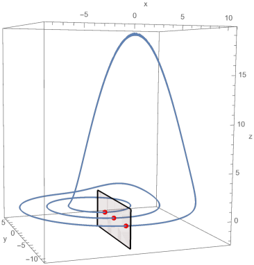
Figure 4. The attracting $3$-periodic orbit for the system (5).

Proof.

Computer-assisted by interval Newton method applied to $P$: [5], Case 1 of the program 01-Roessler_a525.cpp. See also the outline in Appendix, Subsec. 6.1. ∎

Theorem 5.

The Rössler system (5) has $n$-periodic orbits for any $n\in\mathbb{N}$.

Before we present a formal proof we explain the heuristics behind our construction.

We follow the idea of the proof of [18, Th. 2.11]. Assume that there exists a 1-dimensional manifold $\mathcal{M}\subset\Pi$ with boundary (or simply a homeomorphic image of a closed interval), such that $\mathcal{O}^{3}\subset\mathcal{M}$ and apparently $P(\mathcal{M})$ is contained in a small neighbourhood of $\mathcal{M}$ (see Fig. 5).

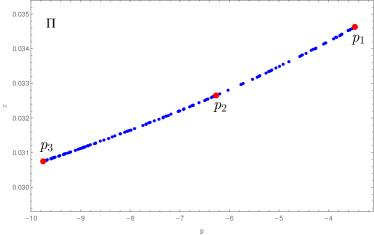
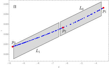
Figure 5. To the left: the fragment of $\Pi$ section containing the $3$-periodic orbit $\mathcal{O}^{3}$ (red) and some orbits attracted by it. The attracted orbits sketch the shape of the hypothetical $1$-dim manifold $\mathcal{M}$.
To the right: the location of the sets $L_{0}$, $L_{1}$ relative to the orbit $\mathcal{O}^{3}$.

Considering Fig. 5, we see that it is reasonable to parameterize $\mathcal{M}$ by the $y$ coordinate. We can now try to make a numerical ‘plot’ of $\mathcal{M}$’s self map $\mathcal{P}$ (a model map for $P$), using the $y$ coordinates of the attracted orbits:

$$y\mapsto\pi_{y}P(y,z)=:\mathcal{P}(y)\text{,\quad where $(y,z)$ apparently belongs to $\mathcal{M}$,}$$

as on Fig. 6.

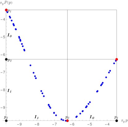
Figure 6. The images of the points near $\mathcal{M}$ through $P$ sketch the plot of the model map $\mathcal{P}$.

Let us denote the ‘segment’ $[p_{1}^{3},p_{2}^{3}]$ by $I_{0}$ and $[p_{2}^{3},p_{3}^{3}]$ by $I_{1}$, as on Fig. 6. Note that $\mathcal{M}$’s segments would fulfil the one-dimensional covering relations:

$$I_{0}\overset{\mathcal{P}}{\longrightarrow}I_{1}\overset{\mathcal{P}}{\longrightarrow}I_{1}\overset{\mathcal{P}}{\longrightarrow}I_{0}.$$

Basing on this observation, we find two-dimensional sets $L_{0}$, $L_{1}$ on $\Pi$, lying close to the segments $I_{0}$, $I_{1}$, which most probably fulfil the similar horizontal covering relations. Their location relative to the orbit $\mathcal{O}^{3}$ is depicted on Fig. 5, to the right. In the proof below we show that these horizontal covering relations indeed occur.

Proof.

Let $M=\begin{bmatrix}-1&0.000706767\\ -0.000706767&-1\end{bmatrix}$ and (with some abuse of notation) $p_{2}^{3}=\begin{bmatrix}-6.264007533274157\\ 0.03265435884602701\end{bmatrix}$. Define an affine map $C$ on $\mathbb{R}^{2}$ by

$$C(x)=Mx+p_{2}^{3}.$$

The matrix $M$ is chosen to place the images of horizontal h-sets through $C$ approximately along $\mathcal{M}$. Consider now two h-sets $N_{0},N_{1}\subset\mathbb{R}^{2}$:

(7) $$N_{0} =[-1.23094\pm 1.41278]\times[\pm 7\cdot 10^{-4}]\text{,}$$

$$N_{1} =[1.84699\pm 1.55949]\times[\pm 7\cdot 10^{-4}].$$

Denote their images through $C$ by

$$L_{0}=C(N_{0})\text{, }\qquad L_{1}=C(N_{1})\text{, }$$

and consider these parallelograms as sets on the section $\Pi$ (see Fig. 7).

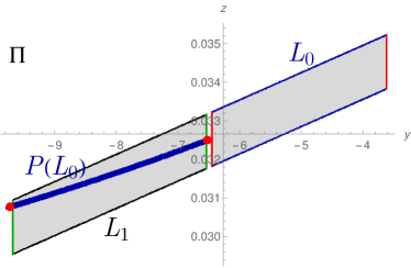
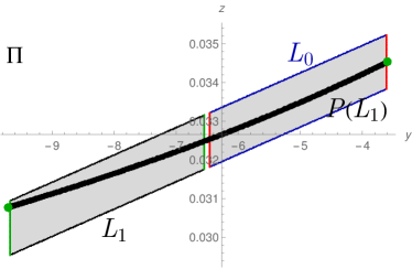
Figure 7. The sets $L_{0}$, $L_{1}$ and their images through $P$. The axes’ origin is moved to the point $p_{2}^{3}$. The sets fulfil $L_{0}\overset{P}{\Longrightarrow}L_{1}\overset{P}{\Longrightarrow}L_{1}\overset{P}{\Longrightarrow}L_{0}$ in an affine coordinate system.

Denote $P_{C}=C^{-1}\circ P\circ C$. Then the following horizontal covering relations occur (from computer-assisted proof [5], Case 2 of the program 01-Roessler_a525.cpp, see also the outline in Appendix, Subsec. 6.2):

$$N_{0}\overset{\text{\raisebox{2.0pt}{$P_{C}$}}}{\Longrightarrow}N_{1}\overset{\text{\raisebox{2.0pt}{$P_{C}$}}}{\Longrightarrow}N_{1}\overset{\text{\raisebox{2.0pt}{$P_{C}$}}}{\Longrightarrow}N_{0}.$$

Now, all periods for $P_{C}$ can be obtained as the loops of horizontal $P_{C}$-covering, as in Theorem 3:

• for $n=1$: the existence of a stationary point follows from the self-covering

  $$N_{1}\overset{P_{C}}{\Longrightarrow}N_{1}\text{;}$$

• for $n\geq 2$: the existence of an $n$-periodic orbit follows from the chain of covering relations:

  $$N_{0}\overset{P_{C}}{\Longrightarrow}N_{1}\underbrace{\overset{P_{C}}{\Longrightarrow}N_{1}\dots\overset{P_{C}}{\Longrightarrow}N_{1}}_{\text{`}\overset{P_{C}}{\Longrightarrow}N_{1}\text{' }n-2\text{ times}}\overset{P_{C}}{\Longrightarrow}N_{0}.$$

  Note that in this case $n$ must be the fundamental period of the point.

Finally, observe that an $n$-periodic orbit for $P_{C}$ defines an $n$-periodic orbit for $P$. ∎

5. Periodic orbits for $a=4.7$

Consider now the system (1) with $a=4.7$, $b=0.2$, that is

(8) $$\begin{cases}x^{\prime}=-y-z,\\ y^{\prime}=0.2\,y+x,\\ z^{\prime}=z(x-4.7)+0.2\end{cases}$$

Our goal is to establish the following result.

Theorem 6.

Consider a parallelogram $\mathcal{A}$ in the $(y,z)$ coordinates on the section $\Pi$ (see Fig. 8):

(9) $$\mathcal{A}=\begin{bmatrix}-6.19384\\ 0.0356629\end{bmatrix}+\begin{bmatrix}-1.&0.000777754\\ -0.000777754&-1.\end{bmatrix}\cdot\begin{bmatrix}\pm 2.66856\\ \pm 4\cdot 10^{-4}\end{bmatrix}.$$

Then $\mathcal{A}$ is forward-invariant for the map $P$, that is

(10) $$P(\mathcal{A})\subset\mathcal{A}\text{,}$$

and the Rössler system (8) has $n$-periodic orbits for any $n\in\mathbb{N}\setminus\{3\}$, passing through $\mathcal{A}$, and it does not have any $3$-periodic orbit there.

Let us comment first the statement about the existence of the forward-invariant $\mathcal{A}$. Such a set was not mentioned in the statement of Theorem 5 because we had proved there the existence of all periods. Now beside the existence of some periodic points we also want to exclude the period $3$, and for this we need to be precise about where this exclusion happens.

The proof relies on several lemmas.

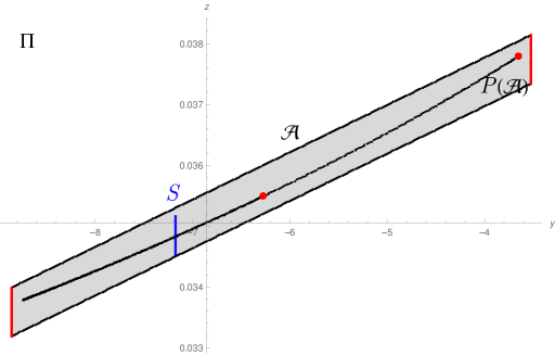
Figure 8. The forward-invariant set $\mathcal{A}$ containing an attractor for the system (8), and its image through $P$. The blue rectangle $S$ contains a stationary point.

From the bifurcation diagram (Fig. 1) it is apparent that there exists a $5$-periodic orbit for the system (8) (see Fig. 9), contained in $\mathcal{A}$. As previously, one proves it by interval Newton method [5] (Case 1 of the program 02-Roessler_a47.cpp, see also Appendix, Subsec. 6.1).

Lemma 7.

The Poincaré map $P$ of the system (8) on the section $\Pi$ has a 5-periodic orbit $\mathcal{O}^{5}=\{p_{1}^{5},p_{2}^{5},p_{3}^{5},p_{4}^{5},p_{5}^{5}\}$, contained in the following rectangles in the $(y,z)$ coordinates on the section $\Pi$:

(11) $$p_{1}^{5}\in -3.885277116_{910041}^{888829}\times 0.037558391444_{32487}^{85094},$$

$$p_{2}^{5}\in -6.8582604471_{62484}^{26429}\times 0.03505366666_{495363}^{561609},$$

$$p_{3}^{5}\in -7.7666312453_{92379}^{48371}\times 0.034417133928_{18681}^{63033},$$

$$p_{4}^{5}\in -5.895584354_{611225}^{509201}\times 0.03578591178_{706747}^{835873},$$

$$p_{5}^{5}\in -8.7223960200_{73123}^{49997}\times 0.033796299364_{04972}^{3551}.$$

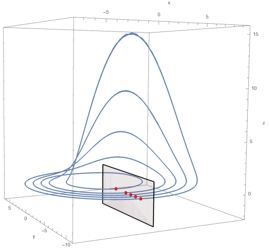
Figure 9. The attracting $5$-periodic orbit for the system (8).

Lemma 8.

The Rössler system (8) has $n$-periodic orbits for any $n\in\mathbb{N}\setminus\{4,3,2\}$.

Heuresis.

Similarly as in the proof of Theorem 5, consider a hypothetical 1-dimensional manifold $\mathcal{M}\subset\Pi$ containing $\mathcal{O}^{5}$ and its self-map, for which the Poincaré map $P$ is a 2-dimensional perturbation (see Fig. 10).

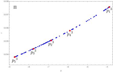
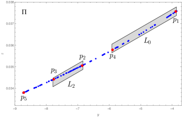
Figure 10. To the left: The fragment of $\Pi$ section containing the $5$-periodic orbit $\mathcal{O}^{5}$, marked in red. Some orbits attracted by $\mathcal{O}^{5}$ allow to estimate the shape of $\mathcal{M}$.
To the right: The location of the sets $L_{0}$, $L_{2}$ relative to the orbit $\mathcal{O}^{5}$.

Let us now parameterize $\mathcal{M}$ by the $y$ coordinate and consider, as previously, the ‘plot’ of the model map $\mathcal{P}:\mathcal{M}\to\mathcal{M}$. Denote the four ‘segments’ of $\mathcal{M}$ by $I_{0}$, $I_{1}$, $I_{2}$ and $I_{3}$, as depicted on Fig. 11.

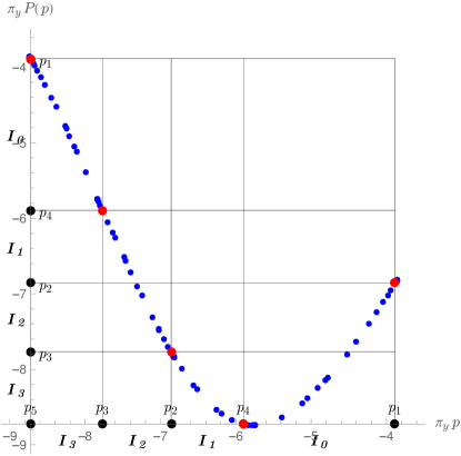
Figure 11. The images of the points near $\mathcal{M}$ through the model map $\mathcal{P}$.

In this case, $\mathcal{M}$’s segments fulfil the following diagram of one-dimensional covering relations:

(12)

In particular, the following chain of covering relations occurs:

$$I_{0}\overset{\mathcal{P}}{\longrightarrow}I_{2}\overset{\mathcal{P}}{\longrightarrow}I_{2}\overset{\mathcal{P}^{3}}{\longrightarrow}I_{0}.$$

Similarly as before, we find two-dimensional sets $L_{0}$, $L_{2}$ on $\Pi$, close to the segments $I_{0}$, $I_{2}$, which are expected to fulfil the analogous horizontal covering relations. One can compare their positions to the orbit $\mathcal{O}^{5}$ on Fig. 10, to the right. Further we will see the proof of these horizontal covering relations.

Proof.

Let $M=\begin{bmatrix}-1&0.000842495\\ -0.000842495&-1\end{bmatrix}$ and $p_{2}^{5}=\begin{bmatrix}-6.858260447127058\\ 0.03505366666527084\end{bmatrix}$. Define an affine map $C$ on $\mathbb{R}^{2}$ by $C(x)=Mx+p_{2}^{5}$ and denote $P_{C}=C^{-1}\circ P\circ C$. As before, the map $C$ is chosen to straighten approximately the set $\mathcal{M}$. Consider now two h-sets $N_{0},N_{2}\subset\mathbb{R}^{2}$:

(13) $$N_{0} =[-1.96783\pm 1.02]\times[\pm 2\cdot 10^{-4}]\text{,}$$

$$N_{2} =[0.454186\pm 0.476895]\times[\pm 2\cdot 10^{-4}].$$

Denote their images through $C$ by $L_{0}=C(N_{0})$ and $L_{2}=C(N_{2})$, and consider these parallelograms as sets on the section $\Pi$ (see Fig. 10, to the right). Compare also to Fig. 12, where the images of $L_{0}$, $L_{2}$ on the $\Pi$ section are depicted.

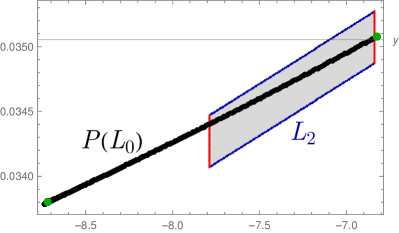
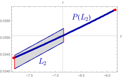
Figure 12. The sets $L_{0}$, $L_{2}$ and their images through $P$ and $P^{3}$. The axes’ origin is moved to the point $p_{2}^{5}$. The sets fulfil $L_{0}\overset{P}{\Longrightarrow}L_{2}\overset{P}{\Longrightarrow}L_{2}\overset{P^{3}}{\Longrightarrow}L_{0}$ in an affine coordinate system.

Let $P_{C}=C^{-1}\circ P\circ C$. Then the following horizontal covering relations occur (from computer-assisted proof [5], Case 2 of the program 02-Roessler_a47.cpp, see also the outline in Appendix, Subsec. 6.2):

$$N_{0}\overset{\text{\raisebox{2.0pt}{$P_{C}$}}}{\Longrightarrow}N_{2}\overset{\text{\raisebox{2.0pt}{$P_{C}$}}}{\Longrightarrow}N_{2}\overset{\text{\raisebox{2.0pt}{$P_{C}^{3}$}}}{\Longrightarrow}N_{0}.$$

Now, we obtain all desired periods for $P_{C}$ as the loops of horizontal $P_{C}$-covering, as in Theorem 3:

• for $n=1$: the existence of a stationary point follows from the self-covering

  $$N_{2}\overset{P_{C}}{\Longrightarrow}N_{2}\text{;}$$

• for $n\geq 5$: the existence of an $n$-periodic orbit follows from the chain of covering relations:

  $$N_{0}\overset{P_{C}}{\Longrightarrow}N_{2}\underbrace{\overset{P_{C}}{\Longrightarrow}N_{2}\dots\overset{P_{C}}{\Longrightarrow}N_{2}}_{\text{`}\overset{P_{C}}{\Longrightarrow}N_{2}\text{' }n-4\text{ times}}\overset{P_{C}^{3}}{\Longrightarrow}N_{0}.$$

  Also in this case $n$ must be the fundamental period of the point.

An $n$-periodic orbit for $P_{C}$ defines an $n$-periodic orbit for $P$, so we get all periods $n$ for $n\in\mathbb{N}\setminus\{2,3,4\}$. ∎

To complete the study, we find also $2$- and $4$-periodic orbits. Note that from Fig. 11 and diagram (12) we expect that for the model map $\mathcal{P}$:

$$I_{0}\overset{\mathcal{P}^{2}}{\longrightarrow}I_{0}\text{, \quad and \quad}I_{1}\overset{\mathcal{P}^{4}}{\longrightarrow}I_{1}\text{,}$$

therefore we may look for a $2$-periodic point on the segment $I_{0}$ and for a $4$-periodic point on $I_{1}$.

Lemma 9.

1. The Poincaré map $P$ of the system (8) on the section $\Pi$ has a 2-periodic orbit $\mathcal{O}^{2}=\{p_{1}^{2},p_{2}^{2}\}$, contained in the following rectangles in the $(y,z)$ coordinates on the section $\Pi$:

   (14) $$p_{1}^{2}\in -4.88392425874_{3846}^{2264}\times 0.0366312810972_{0363}^{9599},$$

   $$p_{2}^{2}\in -8.22095155223_{5825}^{3453}\times 0.0341162008426_{8562}^{9375}.$$

2. The Poincaré map $P$ of the system (8) on the section $\Pi$ has a 4-periodic orbit $\mathcal{O}^{4}=\{p_{1}^{4},p_{2}^{4},p_{3}^{4},p_{4}^{4}\}$, contained in the following rectangles in the $(y,z)$ coordinates on the section $\Pi$:

   (15) $$p_{1}^{4}\in -6.3322511801_{91433}^{86209}\times 0.035445799547_{48502}^{86024},$$

   $$p_{2}^{4}\in -8.4703436541_{25783}^{19862}\times 0.033955548564_{30393}^{40434},$$

   $$p_{3}^{4}\in -4.3626672599_{1514}^{017}\times 0.037102455850_{53683}^{75971},$$

   $$p_{4}^{4}\in -7.5716695403_{62099}^{41765}\times 0.0345497016342_{597}^{7861}.$$

Proof.

Computer-assisted [5], Cases 3 and 4 of the program 02-Roessler_a47.cpp. See also the outline in Appendix, Subsec. 6.1. ∎

Proof of Theorem 6.

First we verify the forward invariance of $\mathcal{A}$: [5], Case 5 of the program 02-Roessler_a47.cpp (see also the outline in Appendix, Subsec. 6.4).

From Lemmata 8 and 9 we have already $n$-periodic orbits for $n\in\mathbb{N}\setminus\{3\}$ in $\mathcal{A}$. It remains to prove that there is no $3$-periodic orbit for $P$ in $\mathcal{A}$. We verify that by the interval Newton method applied to $P$ and $P^{3}$: [5], Case 6 of the program 02-Roessler_a47.cpp (see also the outline in Appendix, Subsec. 6.4). ∎

6. Appendix. Outlines of computer-assisted proofs [5]

We use the CAPD library for C++ [8] containing, in particular, modules for interval arithmetic, linear algebra, differentiation and integration of ODEs. The important utility of the library is calculating Poincaré maps rigorously: we are able to enclose the image of an interval vector (a rectangle $R$, in our case) through $P$ in an interval vector, denoted below by $[P(R)]$. Applying suitable affine coordinate systems helps to reduce the wrapping effect. If that is not enough and the estimated images are too large, we also often divide the sets into grids of smaller boxes and use the fact that the image of the whole set must be contained in the sum of small boxes’ images.

The programs have been tested under Linux Mint 18.1 with gcc compiler. They use the CAPD library ver. 5.0.6. All cases execute within seconds on a laptop type computer with Intel Core i7 2.7GHz $\times$ 2 processor (Case 6 of the program 02-Roessler_a47.cpp takes the longest time: no more than 10 seconds).

6.1. Detecting stationary points for a Poincaré map’s $n$th iterate $P^{n}$

The outline refers to the following proofs:

• existence of a $3$-periodic orbit for $P$, $a=5.25$ (Lemma 4)
  – Case 1 of the program 01-Roessler_a525.cpp;

• existence of a $5$-periodic orbit for $P$, $a=4.7$ (Lemma 7)
  – Case 1 of the program 02-Roessler_a47.cpp;

• existence of $2$- and $4$-periodic orbits for $P$, $a=4.7$ (Lemma 9)
  – Cases 3 and 4 of the program 02-Roessler_a47.cpp.

Outline of the computer-assisted proof.

1. We define the system and a starting point $x_{0}$ close to the expected periodic point;

2. We apply the function anyStationaryPoint, which:

   • initially iterates the interval Newton operator (INO)

     $$N(x_{0},X)=x_{0}-[DP^{n}(X)]^{-1}P^{n}(x_{0})$$

     in a small neighbourhood $X$ of $x_{0}$ to get a better starting point (this step is not necessary, but we finally obtain a better approximation of the periodic point);

   • finally applies INO on the small neighbourhood of the better starting point: if the image $N$ is contained in the interior of the neighbourhood, then a unique stationary point exists in it.

   • returns $N$.

3. Finally we apply a given iteration of $P$ to $N$, to print the whole orbit.

6.2. Horizontal covering relations between h-sets on the section $\Pi$ for the Poincaré map $P$ or its higher iterate

The outline refers to the following proofs:

• the chain of covering relations $N_{0}\overset{\text{\raisebox{2.0pt}{$P_{C}$}}}{\Longrightarrow}N_{1}\overset{\text{\raisebox{2.0pt}{$P_{C}$}}}{\Longrightarrow}N_{1}\overset{\text{\raisebox{2.0pt}{$P_{C}$}}}{\Longrightarrow}N_{0}$ (Theorem 5)
  – Case 2 of the program 01-Roessler_a525.cpp;

• the chain of covering relations $N_{0}\overset{\text{\raisebox{2.0pt}{$P_{C}$}}}{\Longrightarrow}N_{2}\overset{\text{\raisebox{2.0pt}{$P_{C}$}}}{\Longrightarrow}N_{2}\overset{\text{\raisebox{2.0pt}{$P_{C}^{3}$}}}{\Longrightarrow}N_{0}$ (Theorem 6)
  – Case 2 of the program 02-Roessler_a47.cpp;

Outline of the computer-assisted proof.

1. We define the system and the h-sets with their affine coordinate systems;

2. We apply the function covers2D, which checks the conditions from Definition 3 for the estimated images of the h-sets and their vertical edges;

3. If the conditions are fulfilled, then the function returns true.

See also a similar method for 2-dimensional covering described in [6].

6.3. Forward invariance of the set $\mathcal{A}$

The outline refers to the case of the Poincaré map $P$, $a=4.7$ and the set $\mathcal{A}$ from Theorem 6) – Case 5 of the program 02-Roessler_a47.cpp.

Outline of the computer-assisted proof.

1. We define the set $\mathcal{A}$ with its affine coordinate system;

2. We apply the function inside, which divides $\mathcal{A}$ into small boxes $A_{i}$ and checks if each $A_{i}$ is mapped to the interior of $\mathcal{A}$.

3. If the above condition is fulfilled, then the function returns true.

6.4. Non-existence of the $3$-periodic point for the Poincaré map $P$ in the set $\mathcal{A}$

The outline refers to the case of the Poincaré map $P$, $a=4.7$ and the set $\mathcal{A}$ from Theorem 6) – Case 6 of the program 02-Roessler_a47.cpp.

Outline of the computer-assisted proof.

1. We define the set $\mathcal{A}$ with its affine coordinate system;

2. We apply the function whatIsNotMappedOutside, which:

   • divides $\mathcal{A}$ into $500\times 10$ small boxes $A_{i}$

   • checks if each image $[P^{3}(A_{i})]\cap A_{i}=\varnothing$

   • returns a set $S$, which is an interval closure of the sum of all $A_{i}$’s such that $[P^{3}(A_{i})]\cap A_{i}\neq\varnothing$ (see on Fig. 8):

     $$S=-7.1_{86544568881281}^{65195528898398}\times 0.03_{44908202443027}^{522742411001666}.$$

3. We check by interval Newton method (function newtonDivided) that $S$ contains a unique stationary point for $P^{3}$; it still may be in fact a stationary point for $P$.

4. We check by newtonDivided that $S$ contains a unique stationary point also for $P$ and therefore $S$ does not contain any points of fundamental period $3$.

References

- [1] L. Block, J. Guckenheimer, M. Misiurewicz, and L. Young. Periodic points and topological entropy of one dimensional maps. Lecture Notes Math., 819:18, 11 2006.
- [2] Murilo R Cândido, Douglas D Novaes, and Claudia Valls. Periodic solutions and invariant torus in the Rössler system. Nonlinearity, 33(9):4512–4539, Jul 2020.
- [3] CAPD group. Computer Assisted Proofs in Dynamics C++ library. http://capd.ii.uj.edu.pl.
- [4] Z. Galias. Counting low-period cycles for flows. International Journal of Bifurcation and Chaos, 16:2873–2886, 11 2011.
-
[5]
A. Gierzkiewicz and P. Zgliczyński.
C++ source code.
Available online on
http://kzm.ur.krakow.pl/~agierzkiewicz/publikacje.html. - [6] A. Gierzkiewicz and P. Zgliczyński. A computer-assisted proof of symbolic dynamics in Hyperion’s rotation. Celestial Mechanics and Dynamical Astronomy, 131(7), 2019.
- [7] P. Glendinning and C. Sparrow. Local and global behavior near homoclinic orbits. Journal of Statistical Physics, 35:645–696, 1984.
- [8] T. Kapela, M. Mrozek, D. Wilczak, and P. Zgliczyński. CAPD::DynSys: a flexible C++ toolbox for rigorous numerical analysis of dynamical systems. To appear in Communications in Nonlinear Science and Numerical Simulation.
- [9] A. P. Krishchenko. Localization of limit cycles. Differentsial’nye uravneniya, 31(11):1858–1865, 1995.
- [10] M. Morse and G. Hedlund. Symbolic dynamics. Amer. J. Math., 60:815–866, 1938.
- [11] A. Neumaier. Interval Methods for Systems of Equations. Encyclopedia of Mathematics and its Applications. Cambridge University Press, 1991.
- [12] P. Pilarczyk. Topological–numerical approach to the existence of periodic trajectories in ODE’s. Discrete and Continuous Dynamical Systems, 2003, 01 2003.
- [13] O.E. Rössler. An equation for continuous chaos. Physics Letters A, 57(5):397 – 398, 1976.
- [14] A.N. Sharkovskii. Co-existence of cycles of a continuous mapping of the line into itself. Ukrainian Math. J., 16:61–71, 1964. (in Russian, English translation in J. Bifur. Chaos Appl. Sci. Engrg., 5:1263-1273, 1995.).
- [15] P. Stefan. A theorem of Sarkovskii on the existence of periodic orbits of continuous endomorphisms of the real line. Comm. Math. Phys., 54(3):237–248, 1977.
- [16] M. Tërekhin and T. Panfilova. Periodic solutions of the Rössler system. Russian Math. (Iz. VUZ), 43(8):66–69, 1999.
- [17] P. Zgliczyński. Computer assisted proof of chaos in the Rössler equations and in the Hénon map. Nonlinearity, 10(1):243–252, 1997.
- [18] P. Zgliczyński. Multidimensional perturbations of one-dimensional maps and stability of S̆arkovskĭ ordering. International Journal of Bifurcation and Chaos, 09(09):1867–1876, 1999.
- [19] P. Zgliczyński. Sharkovskii theorem for multidimensional perturbations of one-dimensional maps II. Topological Methods in Nonlinear Analysis, 14:169, 09 1999.
- [20] P. Zgliczyński. Sharkovskii’s theorem for multidimensional perturbations of one-dimensional maps. Ergodic Theory and Dynamical Systems, 19(6):1655–1684, 1999.