or with if of and to -off off for in versus subject the
\titlecapoptimal network topology of multi-agent systems subject to computation and communication latency (with proofs)*
Abstract
We study minimum-variance feedback-control design for a networked control system with retarded dynamics, where inter-agent information exchange is subject to latency. We prove that such a control design can be solved efficiently for circular formations and compute near-optimal control gains in closed form. Also, we show that the centralized control is in general a poor design choice when adding communication links to the network increases the latency, and propose a control-driven optimization of the network topology.
Index Terms:
Communication latency, Decentralized control, Feedback latency, Minimum-variance control, Multi-agent systems, Networked control systems.10(2,-4.5)
©2021 IEEE.
Personal use of this material is permitted.
Permission from IEEE must be obtained for all other uses, in any current or future media, including reprinting/republishing this material for advertising or promotional purposes, creating new collective works, for resale or redistribution to servers or lists, or reuse of any copyrighted component of this work in other works.
{textblock}10(2,-3.5)
This paper has been accepted for the 29th Mediterranean Conference on Control and Automation.
Please cite the paper as: L. Ballotta, M. R. Jovanović, and L. Schenato,
“Optimal Network Topology of Multi-Agent Systems subject to Computation and Communication Latency”,
29th Mediterranean Conference on Control and Automation (MED), 2021.
I Introduction
Large-scale networked control systems have been scaling up both in terms of number of agents and spatial distribution over the last years, taking advantage of new communication protocols for massive systems, e.g., 5G [17, 5], and of advances in embedded electronics [25] enhancing the computing performance of the network agents [26, 23]. Indeed, distributed sensing and computation represent the true asset of such systems, whose tasks would otherwise be infeasible. Since the concept of multi-agent systems was introduced to the literature, decentralized control techniques have been developed to adapt classical approaches to network applications [3]. A few examples can be found in control of vehicular formations [7, 10] and of traffic congestion in vehicular networks [12], ground and aerial robot swarms [27, 22, 16] and UAV-UGV cooperative teams [1].
One of the main issues in multi-agent systems is latency, due to communication constraints, limited computational power, or delayed sensing and actuation. In particular, limited bandwidth and finite channel capacity pose a practical limitation to the scalability of large-scale systems and when the information exchange among agents involves heavy data, as with multimedia or in federated learning [24, 20].
Several works deal with decentralized control in the presence of latency. [9, 8] design control laws with convergence conditions for platoons under various network topologies. [28, 29] study consensus of multi-agent systems with time-delays, showing its dependence on parameters such as dynamics and communication graph and giving conditions for mean-square stability. [21] is concerned with finite-time stability of discrete-time neutral-delay systems.
Drawing inspiration from this approach, we design minimum-variance control of networked systems where the information exchange among agents is subject to latency, and we assume that the delays increase with the number of links. Such a situation occurs, e.g., when the total bandwidth available to the network is fixed a priori [11], so that additional links reduce the bandwidth for all communications, or when multi-hop transmissions yield cumulative delays [14]. Also, we demonstrate that adding links beyond a certain threshold worsens the performance, because the latency increase overtakes the benefit accrued by a larger amount of feedback information. In particular, centralized control (the complete graph) is in general a poor choice. To the best of our knowledge, this analysis is new in the existing literature.
To approach such control design in the presence of latency, we consider circular formations. Such systems are deployed for, e.g., source seeking by smart mobile sensors [19, 6] or target tracking by robots [2, 18]. This allows to get analytical results which give insights on the design, while extension to more general topologies is straightforward.
I-A contribution and paper outline
The paper is organized as follows. Section II introduces the system model, detailing results on circular formations (Section II-B) and delay systems (Section II-C). Section III formalizes the control problem: namely, we optimize the feedback gains in order to minimize the steady-state scalar variance of the system. We first solve the problem with a single parameter (equal gains) in Section III-A and then let multiple parameters in Section III-B. In the latter, we prove that an efficient solution coincides with a particular single-parameter configuration. In Section IV, we discuss the control performance under varying network topologies, proposing an optimization that takes into account how the delays increase with the number of links. Specifically, we show that using all communication links (centralized control) yields in general poor performance. Finally, concluding remarks are drawn in Section V, together with proposals for further study.
II setup
II-A system model
We consider a circular formation composed of agents, where each agent is modeled as a single integrator:
| (1) |
where are the state and the control input of agent at time , respectively, and is a standard Brownian motion. Each agent computes its control input exploiting the mismatches between its own state (measured) and other agents’ states (received via wireless).
Assumption 1.
Agent receives state measurements from the agent pairs located positions ahead and behind, . Measurements are received after the delay from the corresponding state sampling, where is a non-decreasing sequence and is a constant.
Remark 1.
The time embeds both the communication delay, due to channel constraints, and the computation delay, arising if the agents preprocess the acquired measurements. In practice, is to be estimated or learned from data.
The control input at time has the following structure:
| (2a) | |||
| (2b) |
where is the desired reference (feedforward control input), is the feedback control input for agent , is -th the feedback gain, , and
| (3) |
are the state mismatches computed with the received measurements,
which in (2b) are delayed according to 1.
System (1)–(2) can be modeled in vector-matrix form as
| (4) |
where is the vector of all ones of dimension , contains the stacked states of all agents at time , and . Denoting the gain vector as , the circulant feedback matrix can be written as
| (5a) | |||
| (5b) |
where is the circulant matrix with the vector as first row. For example, if and ,
| (6) |
II-B decoupling the error dynamics
Let us decompose the state as , where all components of equal the mean of and represents the current mismatches of the agents’ states:
| (7) | |||
| (8) |
The mean-vector dynamics equation reads (c.f. (4))
| (9) |
because the columns of belong to the kernel of . The error dynamics is
| (10) | ||||
where . From now on, we focus on system (10).
We exploit symmetry to diagonalize , with orthogonal and -th eigenvalue equal to (c.f. [13])
| (11) |
The dynamics of the new state reads
| (12) |
where with covariance matrix
| (13) |
because the leftmost eigenvector in , associated with , belongs to the kernel of , and all the other eigenvectors in are also in . In particular, the coordinate (i.e., the mean of ), has trivial dynamics and does not affect system (10), whose state coordinates converge to random variables with expectation equal to . For the sake of simplicity, in the following we assume that is zero mean.
II-C minimum-variance control of scalar delay systems
Let us consider the stochastic retarded differential equation
| (14) | ||||
where , is the delay, is standard Brownian noise, and , , is the initial condition.
Theorem 1 (15).
Lemma 1.
The variance in (16) is strictly convex in .
Proof.
Tedious but standard computations yield . See Section -A for details. ∎
Let us consider the scalar system with delayed dynamics
| (18) |
and control input . We wish to design the gain in order to minimize the steady-state variance of . If , the (infeasible) optimum is and can be increased arbitrarily. Instead, if , the following holds.
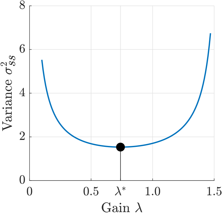
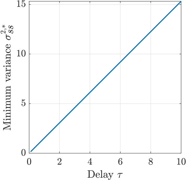
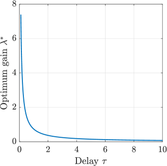
Proposition 1.
Proof.
Setting the derivative of (19) equal to zero leads straightly to (21). See Section -B for details. ∎
III Optimization of feedback gains
In this section, we aim to optimize the feedback gains in (5b) to minimize the steady-state scalar variance of .
Problem 1.
Problem reformulation. In virtue of the change of basis presented in Section II-B, we can write
| (23) |
where the contribution of is neglected in virtue of the trivial dynamics of . Eq. 22 can be rewritten as
| (24) | ||||
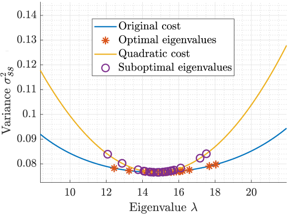
where and the constraint ensures stability (c.f. (15)). In virtue of (11) and Lemma 1, problem (24) is convex and the optimal gains can be found numerically. To achieve analytical intuition, we shift to the (sub-optimal) quadratic optimization of the variance arguments:
| (25) | ||||
The intuition behind the above reformulation is that the quadratic cost function in (25) approximates well the variance in (24) about the minimum (up to scaling and translation). In particular, the spectrum of needs to be “close” to the optimal gain because the variance grows quickly with the smallest and largest eigenvalues (c.f. Fig. 3). Fig. 4 compares the two cost functions in (24)–(25) for , and , together with their optimal eigenvalues in the single-parameter case (see Section III-A).
Remark 2 (Control regularization).
III-A Single parameter
We first impose that all feedback gains are equal to the parameter , such that (5) simplifies to
| (26a) | |||
| (26b) |
and the eigenvectors of are proportional to ,
i.e., , ,
where the coefficients depend on and according to (11).
The variance minimization (22) is reduced to
| (27) | ||||
and the quadratic approximation (25) becomes
| (28) | ||||
Theorem 2.
The solution of (28) is .
Proof.
The result follows by computing the critical points of the cost. See Section -C for details. ∎
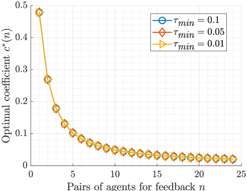
In view of (21), 2 implies that the sub-optimal gain (control effort) decreases as , where the first factor is related to the denser communication topology (more feedback information) and the second, which depends on the delay increase rate , is a direct consequence of the constraint (15) that embeds a stability condition.
III-B multiple parameters
We now let such that can be any vector in .
Theorem 3.
The solution of (25) is .
Proof.
The result follow from properties of the DFT applied to the cost function. See Section -D for details. ∎
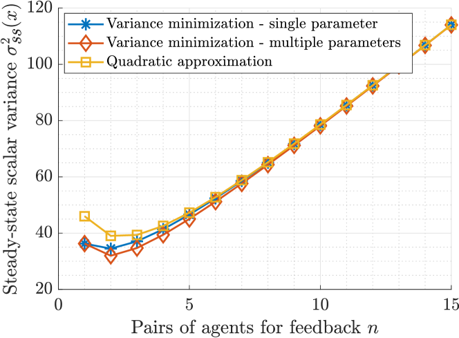
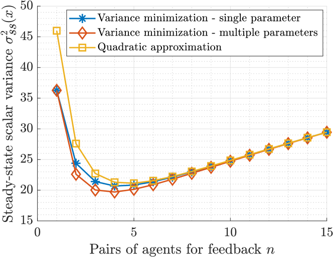
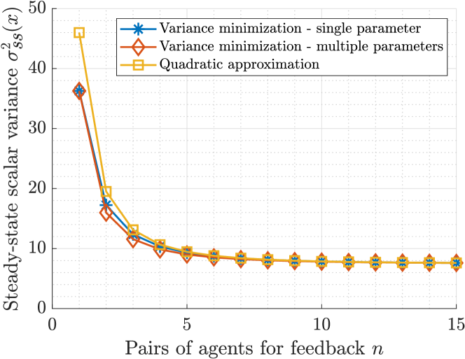
3 states that optimizations (25) and (28) coincide, i.e., choosing the same gain for all agents is a good choice even if different gains are allowed. Fig. 8 compares the scalar variances obtained from the two variance minimizations (27) and (22) and from the quadratic approximation (28) with , and three rates .
IV discussion: the role of latency in decentralized control
The gains obtained by solving 1 or its quadratic approximation (28), and the resulting steady-state variance, depend on the pairs of communicating agents and the delay . The following result quantifies such dependence for the solution of the approximated problem (28).
Proposition 2.
The scalar variance can be written as
| (30) |
where does not depend on and can be computed exactly. The network topology is optimized by
| (31) |
Proof.
The result follows from straightforward manipulations of the analytical expression of . See Section -E for details. ∎
Given how is computed, characterizing analytically is hard. Numerical tests show that is submodular decreasing and that the steady-state variance has a unique point of minimum when is discrete-concave, as shown in Fig. 8. Eq. 30 suggests that the optimal number of links is smaller than or equal to the maximum, i.e., , with the centralized control (corresponding to the complete graph, ) performing poorly in general. Also, depends on the rate in a “non-increasing” fashion, namely, slower rates yield larger optima. For example, the optimal number of links is greater with (, Fig. 8) than with (, Fig. 8). Centralized control is optimal when the delay is constant (Fig. 8), because in this case adding links does not penalize the dynamics.111Although the same holds true with , in this case the computations in Appendix E cannot be applied.
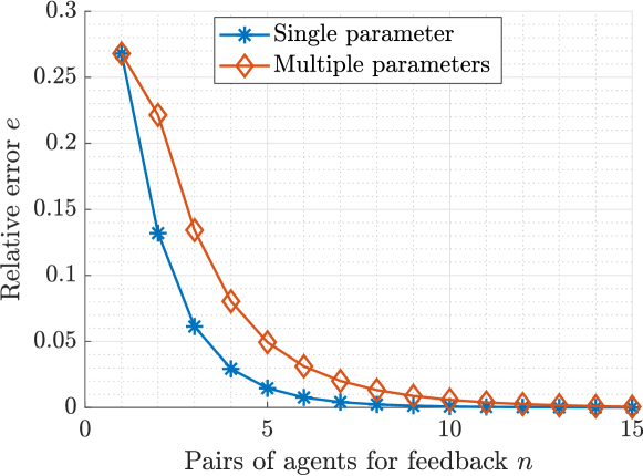
What discussed so far involves the performance when the gains are computed according to 2. As shown in the proof of 2, the key argument to (30) is that is linear in through a coefficient that only depends on . Even though proving the same analytically for the optimal gains of 1 is hard, numerical evidence suggests that this is indeed the case. For example, Fig. 10 shows the ratio , which is independent of both and and hence is consistent with the guess . Simulations show that the relative gap depicted in Fig. 9 is also independent of , reinforcing such a hypothesis: in fact, (29) can be rewritten as
| (32) |
only if the optimal variance can be expressed as . This suggests that the minimum variance obtained from (22)–(27) can also be optimized over , as show by Fig. 8, for both the single-gain and multiple-gain designs. The optimal network topology trades the feedback information (maximized by the centralized architecture) for the latency (minimized by the fully distributed control): the optimizer represents a threshold beyond which the benefit of adding communication links is overwhelmed by the delay increase in the retarded dynamics.
Remark 3.
All above results assume a fixed system size for ease of notation. As one can notice from the proof, the coefficient is parametric in , and therefore the optimal values and in (31) also depend on .
Remark 4.
Eq. 30 shows that does not depend on . In particular, the optimal topology is only determined by the delay increase rate and by the system size .
V Conclusions
In this paper, motivated by delay networked control systems, we design minimum-variance feedback control assuming that the latency in information exchange increases with the amount of links, i.e., the number of agents involved in the decentralized feedback loops. Sub-optimal gains, whose performance tends to the optimum as the network topology becomes denser, are characterized by a simple expression. We show that the network topology can be optimized over the number of links, and that centralized control yields poor performance in general. Future improvements might involve a more complex model for the system dynamics or heterogeneous agents with different delays.
-A Proof of Lemma 1
| (33) |
Because does not impact convexity, we let . The second derivative of , written in (33) in the next page, is positive if
| (34) |
The constraint (15) ensures that , and are positive. We now consider three cases for and show that the negative terms in (34) are always outbalanced by the positive terms.
- :
-
(35) (36) - :
-
(37) (38) - :
-
(39) (40)
-B Proof of 1
-C Proof of 2
According to (11), we first rewrite each eigenvalue as . The cost function in (28) can then be rewritten as
| (43) |
We first exploit strict convexity to find the global minimum of (43). To this aim, we set
| (44) |
which admits the unique solution
| (45) |
The coefficients are the eigenvalues of when . Because the eigenvalues of a circulant matrix are the Discrete Fourier Transform (DFT) of its first row, we can write
| (46) | |||
| (47) |
where is the first row of , (46) comes from the definition of inverse DFT and (47) from Plancherel theorem.
The final expression of follows by substituting (46)–(47) in (45).
We now need to check if such solution satisfies the constraint.
We first note that
by studying the sign of (41). We then have the following relations for the maximum eigenvalue:
| (48) | ||||
-D Proof of 3
Exploiting linearity of the DFT and Plancherel theorem, problem (25) can be recast as follows:
| (49) | ||||
where is the first row of and is the -th canonical vector in . Given , consider now the problem
| (50) | ||||
with and . We show that , which implies that the optimal gains in are equal. Assume there exists such that for all . The cost of is
| (51) |
Let such that , for all . We have
| (52) | ||||
and the cost associated with is
| (53) |
We then have the following chain of inequalities:
| (54) | ||||
which implies for any .
The statement follows from optimality of in (28).
-E Proof of 2
The proof follows straightforward manipulations of the analytical expression of . From (23), we have
| (55) |
where are the near-optimal eigenvalues (c.f. Appendix -C). Consider the formula in 2 for the gain , which we rewrite as . Then, each variance can be written as follows:
| (56) | ||||
where (21) has been used, and multiplies in the third line of (56). The scalar variance can then be written as
| (57) |
where .
References
- [1] Barbara Arbanas, Antun Ivanovic, Marko Car, Matko Orsag, Tamara Petrovic, and Stjepan Bogdan. Decentralized planning and control for uav–ugv cooperative teams. Autonomous Robots, 42(8):1601–1618, 2018.
- [2] Lara Brinón Arranz, Alexandre Seuret, and Carlos Canudas De Wit. Translation control of a fleet circular formation of auvs under finite communication range. In Proceedings of the 48h IEEE Conference on Decision and Control (CDC) held jointly with 2009 28th Chinese Control Conference, pages 8345–8350. IEEE, 2009.
- [3] Lubomír Bakule. Decentralized control: An overview. Annual Reviews in Control, 32(1):87 – 98, 2008.
- [4] Luca Ballotta, Mihailo R. Jovanović, and Luca Schenato. Optimal Network Topology of Multi-Agent Systems subject to Computation and Communication Latency. arXiv e-prints, page arXiv:2101.10394, January 2021.
- [5] Andrea Biral, Marco Centenaro, Andrea Zanella, Lorenzo Vangelista, and Michele Zorzi. The challenges of m2m massive access in wireless cellular networks. Digital Communications and Networks, 1(1):1–19, 2015.
- [6] Lara Briñón-Arranz, Luca Schenato, and Alexandre Seuret. Distributed source seeking via a circular formation of agents under communication constraints. IEEE Transactions on Control of Network Systems, 3(2):104–115, 2015.
- [7] Hossein Chehardoli and Ali Ghasemi. Adaptive centralized/decentralized control and identification of 1-d heterogeneous vehicular platoons based on constant time headway policy. IEEE Transactions on Intelligent Transportation Systems, 19(10):3376–3386, 2018.
- [8] Hossein Chehardoli and Ali Ghasemi. Formation control of longitudinal vehicular platoons under generic network topology with heterogeneous time delays. Journal of Vibration and Control, 25(3):655–665, 2019.
- [9] F. de Oliveira Souza, L. A. B. Torres, L. A. Mozelli, and A. A. Neto. Stability and formation error of homogeneous vehicular platoons with communication time delays. IEEE Transactions on Intelligent Transportation Systems, 21(10):4338–4349, 2020.
- [10] Ioannis M Delimpaltadakis, Charalampos P Bechlioulis, and Kostas J Kyriakopoulos. Decentralized platooning with obstacle avoidance for car-like vehicles with limited sensing. IEEE Robotics and Automation Letters, 3(2):835–840, 2018.
- [11] Eloy Garcia, Yongcan Cao, and David W Casbeer. Periodic event-triggered synchronization of linear multi-agent systems with communication delays. IEEE Transactions on Automatic Control, 62(1):366–371, 2016.
- [12] H. Günther, R. Riebl, L. Wolf, and C. Facchi. Collective perception and decentralized congestion control in vehicular ad-hoc networks. In 2016 IEEE Vehicular Networking Conference (VNC), pages 1–8, 2016.
- [13] Robert M. Gray. Toeplitz and circulant matrices: A review. Foundations and Trends® in Communications and Information Theory, 2(3):155–239, 2006.
- [14] Gagan Rajesh Gupta and Ness Shroff. Delay analysis for multi-hop wireless networks. In IEEE INFOCOM 2009, pages 2356–2364. IEEE, 2009.
- [15] Uwe Küchler and Beatrice Mensch. Langevins stochastic differential equation extended by a time-delayed term. Stochastics and Stochastic Reports, 40(1-2):23–42, 1992.
- [16] Hanjun Li, Chunhan Feng, Henry Ehrhard, Yijun Shen, Bernardo Cobos, Fangbo Zhang, Karthik Elamvazhuthi, Spring Berman, Matt Haberland, and Andrea L Bertozzi. Decentralized stochastic control of robotic swarm density: Theory, simulation, and experiment. In 2017 IEEE/RSJ International Conference on Intelligent Robots and Systems (IROS), pages 4341–4347. IEEE, 2017.
- [17] Shancang Li, Li Da Xu, and Shanshan Zhao. 5g internet of things: A survey. Journal of Industrial Information Integration, 10:1–9, 2018.
- [18] Lili Ma and Naira Hovakimyan. Cooperative target tracking in balanced circular formation: Multiple uavs tracking a ground vehicle. In 2013 American Control Conference, pages 5386–5391. IEEE, 2013.
- [19] Brandon J Moore and Carlos Canudas-de Wit. Source seeking via collaborative measurements by a circular formation of agents. In Proceedings of the 2010 American control conference, pages 6417–6422. IEEE, 2010.
- [20] Emre Ozfatura, Baturalp Buyukates, Deniz Gunduz, and Sennur Ulukus. Age-Based Coded Computation for Bias Reduction in Distributed Learning. arXiv e-prints, page arXiv:2006.01816, June 2020.
- [21] Hangli Ren, Guangdeng Zong, Linlin Hou, and Yi Yang. Finite-time resilient decentralized control for interconnected impulsive switched systems with neutral delay. ISA transactions, 67:19–29, 2017.
- [22] Fabrizio Schiano, Antonio Franchi, Daniel Zelazo, and Paolo Robuffo Giordano. A rigidity-based decentralized bearing formation controller for groups of quadrotor uavs. In 2016 IEEE/RSJ International Conference on Intelligent Robots and Systems (IROS), pages 5099–5106. IEEE, 2016.
- [23] Weisong Shi, Jie Cao, Quan Zhang, Youhuizi Li, and Lanyu Xu. Edge computing: Vision and challenges. IEEE internet of things journal, 3(5):637–646, 2016.
- [24] Wenqi Shi, Sheng Zhou, Zhisheng Niu, Miao Jiang, and Lu Geng. Joint device scheduling and resource allocation for latency constrained wireless federated learning. IEEE Transactions on Wireless Communications, 20(1):453–467, 2020.
- [25] Amr Suleiman, Zhengdong Zhang, Luca Carlone, Sertac Karaman, and Vivienne Sze. Navion: A fully integrated energy-efficient visual-inertial odometry accelerator for autonomous navigation of nano drones. In 2018 IEEE Symposium on VLSI Circuits, pages 133–134. IEEE, 2018.
- [26] Shanhe Yi, Cheng Li, and Qun Li. A survey of fog computing: concepts, applications and issues. In Proceedings of the 2015 workshop on mobile big data, pages 37–42, 2015.
- [27] Quan Yuan, Jingyuan Zhan, and Xiang Li. Outdoor flocking of quadcopter drones with decentralized model predictive control. ISA transactions, 71:84–92, 2017.
- [28] X. Zong, T. Li, G. Yin, L. Y. Wang, and J. Zhang. Stochastic consentability of linear systems with time delays and multiplicative noises. IEEE Transactions on Automatic Control, 63(4):1059–1074, April 2018.
- [29] Xiaofeng Zong, Tao Li, and Ji-Feng Zhang. Consensus conditions of continuous-time multi-agent systems with time-delays and measurement noises. Automatica, 99:412 – 419, 2019.