An Updated Formalism For Line-Driven Radiative Acceleration and Implications for Stellar Mass Loss

Abstract

Radiation contributes to the acceleration of large-scale flows in various astrophysical environments because of the strong opacity in spectral lines. Quantification of the associated force is crucial to understanding these line-driven flows, and a large number of lines (due to the full set of elements and ionization stages) must be taken into account. Here we provide new calculations of the dimensionless line strengths and associated opacity-dependent force multipliers for an updated list of approximately 4.5 million spectral lines compiled from the NIST, CHIANTI, CMFGEN, and TOPbase databases. To maintain generality of application to different environments, we assume local thermodynamic equilibrium, illumination by a Planck function, and the Sobolev approximation. We compute the line forces in a two-dimensional grid of temperatures (i.e., values between 5,200 and 70,000 K) and densities (varying over 11 orders of magnitude). Historically, the force multiplier function has been described by a power-law function of optical depth. We revisit this assumption by fitting alternative functions that include a saturation to a constant value (Gayley’s $\bar{Q}$ parameter) in the optically-thin limit. This alternate form is a better fit than the power-law form, and we use it to calculate example mass-loss rates for massive main-sequence stars. Because the power-law force multiplier does not continue to arbitrarily small optical depths, we find a sharp decrease, or quenching, of line-driven winds for stars with effective temperatures less than about 15,000 K.

1 Introduction

The study of flows driven by photons has a long history. For example, Johnson (1925) hypothesized that that helium atoms could be ejected from a star via radiation pressure, suggesting that photon-driven flows can be responsible for stellar mass loss. We now know that photon-driven outflows exist in various astrophysical environments, including accreting objects such as protostars, cataclysmic variables, and active galactic nuclei (AGN) (Owocki, 2004; Puls et al., 2008; Higginbottom et al., 2014). The driving mechanism of these flows by photons is often referred to as “radiation pressure,” where the force of radiation from the spectral lines acts on the material of the outflow. The very large number of spectral lines in any given ion has a dominant effect on this pressure on the flow material (Castor, 1974; Castor et al., 1975). The absorption and re-emission of photons in a spectral line of frequency $\nu_{0}$ results in a radial transfer of momentum, driving a wind outward from the star.

Quantifying and understanding mass and energy flows is critical in the understanding of how affected objects evolve and interact with their surroundings. Massive star winds can be directly observed in the stellar spectral energy distributions once the star is above a certain threshold luminosity (Kudritzki & Puls, 2000). Ultraviolet (UV) observations showing P Cygni profiles and high flow velocities initially suggested that an extension of solar wind theory was insufficient to explain the winds of O and B stars (Cassinelli, 1979). Lucy & Solomon (1970) demonstrated that the absorption and re-emission of photons by 12 UV resonance lines can drive a wind in O type stars, consequently driving mass loss in the form of the stellar wind. Castor et al. (1975) (hereafter CAK) found that the large number of lines in any given ion of an atom contribute to the radiation force, proportional to the continuum flux at their specific frequency. Using 900 multiplets of C III, CAK found a mass loss rate estimate $\sim$100 times greater than those predicted by Lucy & Solomon (1970), leading to the conclusion that the force from the lines should exceed gravity by approximately two orders of magnitude for small optical depths in O type stars. Therefore, O stars cannot have static atmospheres, as there is no mechanism that can prevent the ejection of the surface layers of the star. This was a major advancement in the understanding of stellar winds. Models based on the theory of line-driven winds have yielded results that agree well with observations of mass loss and terminal flow rates (Owocki et al., 1988; Puls et al., 2008; Sundqvist et al., 2019).

Line-driven outflows are also encountered in various other environments. For example, broad absorption lines are present in the UV spectra of quasars, as well as in other wavelengths. In these cases, the blueshift of the lines suggests the presence of winds from the AGN, sometimes with velocities of up to $0.2c$, making a line-driven disk wind a promising hydrodynamical scenario for AGN outflows (Proga, 2007; Risaliti & Elvis, 2010). Additionally, Kee et al. (2016) suggested that the strong line-driven winds from OB type stars with circumstellar disks could drive ablation of the disk’s surface layers on short timescales that could be a contributing factor to the relative rarity of O type stars in the galaxy (see also Kee et al., 2018a, Kee et al., 2018b, Kee & Kuiper, 2019). By themselves, winds from massive stars can drive galactic evolution by injecting momentum, energy, and stellar material into the interstellar medium (Kudritzki & Puls, 2000).

Previous authors have computed lists of spectral lines and modeled the distributions of the line strength parameters (see for example Abbott, 1982; Shimada et al., 1994; Gormaz-Matamala et al., 2019). However, these line lists have been comprised of significantly fewer lines than those currently available. Lucy & Solomon (1970) originally used 12 lines, CAK updated this to include 900 transitions, and Pauldrach (1987) used a list of 10,000 transitions. More recently, Gormaz-Matamala et al. (2019) used a list of $\sim$900,000 lines, and Björklund et al. (2020) has used a database of approximately one million lines (see also Sundqvist et al. 2019). In this work we construct a newly updated line list, comprised of 4,514,900 spectral lines. To this end, atomic data is assembled from four separate databases. We also reexamine the validity of the historical assumption of a power law to describe the line strength distribution.

This work primarily aims to provide new insight into the form of the line-force multiplier, beyond that of the CAK power-law form. This new form will also provide an alternative to computationally expensive simulations that use the full line list, such as those described in Gormaz-Matamala et al. (2019). To do this, we make some basic assumptions, such as those of local thermodynamic equilibrium (LTE), and an initial Planck function central source. These assumptions and the calculation process of dimensionless line strengths and weighting functions are described in further detail in Section 2. Section 3 describes the collection and compilation of the spectral lines. Section 4 describes the calculation of the updated force multiplier $M(t)$, as well as the fitting of a CAK-form power-law (Section 4.2) and an alternate function (Section 4.3) to the calculated values. Section 5 describes the calculation of mass-loss rates from both the CAK (Section 5.2) and alternate (Section 5.3) multiplier forms, and a comparison of the two (Section 5.5). We end with a discussion of our conclusions in Section 6.

2 Radiative Acceleration of Line-Driven Flows

A general way of expressing the radiative acceleration ${\bf g}_{\rm rad}$ on a parcel of gas is to take the first moment of the equation of radiative transfer. Following Hubeny & Mihalas (2014),

$${\bf g}_{\rm rad}({\bf r})\,=\,\frac{1}{c}\int d\nu\int d\Omega\hat{\bf n}\,(\kappa_{\nu}I_{\nu}-j_{\nu})$$ (1)

where $\hat{\bf n}$ is the unit vector specifying an arbitrary ray-path, $\kappa_{\nu}$ and $j_{\nu}$ are the absorption coefficient (cm² g^-1) and emissivity, and $I_{\nu}$ is the specific intensity. In the comoving frame of a flow, it is often assumed that $j_{\nu}$ is an even function of $\hat{\bf n}$ (so it cancels out of the above moment integral) and that angle anisotropies of $\kappa_{\nu}$ are sufficiently weak to allow it to be taken out of the solid-angle integral. Thus, the expression we use is

$$\textbf{g}_{\rm rad}(\textbf{r})=\frac{1}{c}\int\kappa_{\nu}\textbf{F}_{\nu}(\textbf{r})d\nu$$ (2)

where ${\bf F}_{\nu}$ is the radiative flux (photon energy flux). Below, we also write the opacity $\chi_{\nu}$ in units of cm^-1 as

$$\chi_{\nu}=\kappa_{\nu}\rho=\sigma_{\nu}n$$ (3)

where it is sometimes useful to use the absorption coefficient $\kappa_{\nu}$ or the cross section $\sigma_{\nu}$, and we also define the mass density $\rho$ and number density $n$ in units of cm^-3.

From Equation (2), we see that opacity is necessary for any acceleration due to the radiation field to occur; with zero opacity, the radiation cannot interact with the material of the flow. Spectral lines have a dramatic effect on the wind driving due to resonance that occurs when encountering continuum photons, leading to a large cross section. This effect can be strong enough that it is still magnified after being averaged over the entire continuum. Therefore, to find the total radiative force on a parcel of gas of given temperature and density, all the spectral lines that are encountered by the radiation field must be accounted for. The inclusion of as many lines as possible is imperative in developing a more complete understanding of this phenomenon.

2.1 Dimensionless Line Strengths

We follow Gayley (1995) in characterizing the distribution of spectral line strengths as a set of dimensionless ratios $q_{i}$ that describe the atomic physics, and dimensionless weighting factors $\widetilde{W}_{i}$ that describe the illumination of the atom from a given spectral energy distribution. The product $q_{i}\widetilde{W}_{i}$ represents the full ratio of radiative acceleration due to a specific line $i$ to the acceleration on free electrons. In such a ratio of accelerations (see Equation (2)), the pre-factors of $1/c$ cancel out, and we choose to multiply both the numerator and denominator by the mass density $\rho$. We can write the bound line opacity as

$$\chi_{\nu}=\chi_{\rm{L}}\phi(\nu)$$ (4)

where $\phi(\nu)$ is the line profile function. Thus, the ratio of accelerations can be written as

$$\frac{g_{\rm bound}}{g_{\rm free}}=\frac{\int\chi_{\nu}F_{\nu}d\nu}{\int\chi_{e}F_{\nu}d\nu}=\frac{\chi_{L}\int\phi(\nu)F_{\nu}d\nu}{\chi_{e}\int F_{\nu}d\nu}.$$ (5)

For this work, we assume that the environments in question are in LTE. This assumption (also used by CAK) is often set aside when modeling line-driven winds from, e.g., massive stars, but here we retain it to maintain a level of generality concerning the environments in question. Of course, this assumption will need to be reevaluated in future applications to specific systems (see, e.g, Pauldrach, 1987). Under the assumption of LTE, the quantity $\chi_{L}$ is then given by

$$\chi_{L}=\frac{\pi e^{2}}{m_{e}c}f_{ij}n_{i}\left(1-e^{-h\nu_{0}/kT}\right),$$ (6)

where $f_{ij}$ is the semiclassical oscillator strength, where $i$ and $j$ are used to refer to the lower and upper atomic levels, respectively. The Thomson scattering opacity $\chi_{e}$ is given by

$$\chi_{e}=\sigma_{T}n_{e}=\left(\frac{8\pi r_{e}^{2}}{3}\right)n_{e}$$ (7)

where $\sigma_{T}$ is the Thomson scattering cross section and the classical electron radius is given by

$$r_{e}=\frac{e^{2}}{m_{e}c^{2}}.$$ (8)

Each line profile function $\phi\nu)$ is very narrow when integrated over the energy distribution, so we can approximate it to a Dirac delta function when evaluated at frequency $\nu_{0}$

$$\int\phi(\nu)F_{\nu}d\nu\approx F_{\nu_{0}}.$$ (9)

We can additionally define the frequency integrated flux $F$ as

$$\int F_{\nu}d\nu\equiv F.$$ (10)

We can then define a dimensionless weighting ratio

$$\widetilde{W}_{i}=\frac{\nu_{0}F_{\nu_{0}}}{F},$$ (11)

which accounts for the flux integrals in Equation (3).

In this paper, we maintain a generality of application by assuming a Planck function for the illuminating flux. We use a temperature $T$, presumed equal to the local temperature of the gas ($T=T_{\rm rad}=T_{\rm eff}$), to characterize this Planck function (Noebauer & Sim, 2015; Gormaz-Matamala et al., 2019). Although some authors have suggested the electron temperature is a fraction (usually 0.8$T_{\rm eff}$) of the effective temperature, the radiative temperature is often taken to be equal to that of $T_{\rm eff}$ in the Planck case (see, for example, Puls et al., 2000). This assumption is commonly used for the wind-driving circumstellar regions near massive-star photospheres (e.g., Drew 1989, Kee et al. 2016), in which radiative cooling in an isothermal gas efficiently maintains a nearly constant temperature $T$, roughly equal to the stellar effective temperature $T_{\rm eff}$. Thus, we specify

$$F_{\nu_{0}}=\frac{2\pi h\nu_{0}^{3}/c^{2}}{e^{h\nu_{0}/k_{\rm B}T}-1},$$ (12)

and the frequency-integrated flux is given by

$$F=\sigma T^{4},$$ (13)

where $\sigma$ is the Stefan-Boltzmann constant. Since these are dependent on the wavelength of the transition, there is a unique weighting parameter $\widetilde{W_{i}}$ for each line in every ion and temperature $T$.

Using Equation (11), we can write the ratio of the bound to free acceleration as

$$\frac{g_{\rm bound}}{g_{\rm free}}=\frac{\chi_{L}}{\chi_{e}}\frac{\widetilde{W}_{i}}{\nu_{0}}=\frac{\chi_{L}}{\chi_{e}}\frac{\lambda_{0}\widetilde{W}_{i}}{c}.$$ (14)

Finally, combining Equations (6), (7), and (14), we have

$$\frac{g_{\rm bound}}{g_{\rm free}}=\frac{3}{8}\frac{\lambda_{0}}{r_{e}}f_{ij}\frac{n_{i}}{n_{e}}\left(1-e^{-h\nu_{0}/k_{\rm B}T}\right)\widetilde{W}_{i},$$ (15)

and we define the dimensionless line strength parameter $q_{i}$ as

$$q_{i}\equiv\frac{3}{8}\frac{\lambda_{0}}{r_{e}}f_{ij}\frac{n_{i}}{n_{e}}\left(1-e^{-h\nu_{0}/k_{\rm B}T}\right).$$ (16)

This is similar to Equation 9 of Gayley (1995). However, here we have included the traditional correction factor for stimulated emission.

We also define the sum of the line strengths $\bar{Q}$ as

$$\bar{Q}=\sum_{i}q_{i}\widetilde{W}_{i}.$$ (17)

2.2 Ionization Equilibrium

In order to calculate Equation (16), we first must first calculate the number density ratio $n_{i}/n_{e}$, which is given by

$$\frac{n_{i}}{n_{e}}=\left(\frac{n_{i}}{n_{\rm ion}}\right)\left(\frac{n_{\rm ion}}{n_{\rm el}}\right)\left(\frac{n_{\rm el}}{n_{H}}\right)\left(\frac{n_{H}}{n_{e}}\right).$$ (18)

In LTE, the total number of particles in the lower transition level can be described as a fraction of the total number of particles in the given ionization state:

$$\frac{n_{i}}{n_{\rm ion}}=\frac{g_{i}e^{-(E_{i}-E_{0})/k_{\rm B}T}}{U_{\rm ion}(T)}.$$ (19)

Here $U_{ion}$ is the ion-specific temperature dependent partition function, $g_{i}$ is the ground state statistical weight, $E_{i}$ is the energy of the lower level of the transition, and $E_{0}$ is the ground level energy, which was set to zero by the atomic databases used here. It should also be noted that the oscillator strength $f_{ij}$ (as in Equation (16)) is needed only to form the product $g_{i}f_{ij}$ (as in Equation (19)) and never appears alone.

The elemental abundance ratio $n_{\rm el}/n_{H}$ was obtained from tabulated solar abundances (Asplund et al., 2009), whereas the other two quantities in parentheses, $n_{\rm ion}/n_{\rm el}$ and $n_{H}/n_{e}$, were found using the Saha equation:

$$\frac{n_{i+1}}{n_{i}}n_{e}=\frac{2}{\lambda_{e}^{3}}\frac{U_{i+1}}{U_{i}}\exp{\left[-\frac{E_{i+1}-E_{i}}{k_{\rm B}T}\right]},$$ (20)

where the thermal de Broglie wavelength of a free electron $\lambda_{e}$ is given by

$$\lambda_{e}=h/\sqrt{2\pi m_{e}k_{\rm B}T}.$$ (21)

To solve Equation (20) for the pairwise ionization fractions $n_{i+1}/n_{i}$, we also need to know the electron number density $n_{e}$. Therefore, we made an initial estimate for $n_{e}$, which was then refined using an undercorrection technique. This was done at the end of each iteration over the Saha equation by tabulating a new estimate of $n_{e}$ from the calculated ionization balance, which was then multiplied by the previous estimate. The square root of this product was then used as the estimate of $n_{e}$ for the next iteration. We found that 20 iterations were sufficient to reach a stable value for $n_{e}$. An example set of calculations is shown in Figure 1, which shows the final converged-upon values of $n_{e}$ for our temperature range, for an example density of $\rho=10^{-13}$ g cm^-3.

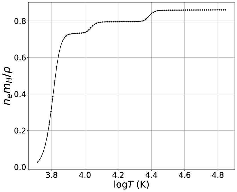
Figure 1: Iterated values of $n_{e}$ as a function of temperature, for $\rho=10^{-13}$ g cm^-3.

The initial estimate for $n_{e}$ was given by

$$n_{e}=0.1\left(\frac{\rho}{m_{H}}\right)$$ (22)

where $\rho$ is the density of the wind and $m_{H}$ is the mass of Hydrogen. For this work, we used a grid of density with 22 values spanning $10^{-20}$ to $10^{-10}$ g cm^-3, a similar density range to that used by Abbott (1982). This broad range is applicable to both massive star winds as well as other astrophysical environments that exhibit line-driven outflows.

The quantity $n_{\rm el}$ can be found from the initial elemental abundances, here taken from Asplund et al. (2009). These are given in the form of number density ratios to the abundance of hydrogen (i.e. $n_{\rm el}/n_{\rm H}$). From these we find the fractional abundance by mass $\mu$ of each element:

$$\mu=\frac{A_{\rm el}\left(n_{\rm el}/n_{\rm H}\right)}{\sum_{\rm el}A_{\rm el}\left(n_{\rm el}/n_{\rm H}\right)}$$ (23)

where $A_{\rm el}$ is the atomic weight of the element. The number density in cm^-3 for each element can then be found from the total mass density $\rho$, the fractional abundance $\mu$, and the mass of hydrogen $m_{\rm H}$:

$$n_{\rm el}=\frac{\rho\mu}{A_{\rm el}m_{\rm H}}.$$ (24)

Knowing $n_{e}$ and the tabulated number density of hydrogen $n_{H}$ from Equations (23)–(24), we can then calculate the quantity $n_{H}/n_{e}$, leaving only the second quantity in Equation (18), $n_{\rm ion}/{n_{\rm el}}$. For ionization stage I this is given by

$$\frac{n_{\rm I}}{n_{\rm el}}=\left[\frac{n_{\rm II}}{n_{\rm I}}+\frac{n_{\rm III}}{n_{\rm II}}\frac{n_{\rm II}}{n_{\rm I}}+...\right]^{-1},$$ (25)

where II and III represent ionization stages I and II of the element in question. Here $n_{\rm I}$ represents $n_{\rm ion}$ as seen in Equation (18). Each fraction in the brackets is given by the Saha equation (Equation (20)). We can similarly isolate $n_{\rm II}/n_{\rm el}$ and the higher ratios to find $n_{\rm ion}/n_{\rm el}$ for any ionization stage, and consequently $n_{\rm ion}/n_{e}$ and $n_{i}/n_{e}$ as in Equation (18), of any element that we consider. Figure 2 shows an example calculation of $n_{\rm ion}/n_{\rm el}$ for the ionization stages of oxygen. These steps were carried out for all elements from H to Ni. We considered all ionization stages for elements with atomic numbers $Z\leq 10$, and only the first ten ionization stages for elements with $Z>10$.

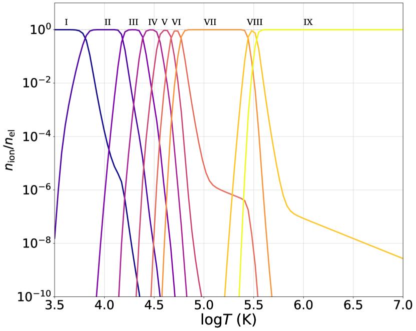
Figure 2: The ionization fraction $n_{\rm ion}/n_{\rm el}$ for the ionization stages of oxygen, for a fixed wind density of $\rho=10^{-13}$ g cm^-3.

3 Atomic Data

3.1 Partition Functions

The LTE partition functions used in Equations (19)–(20) were calculated according to the fitting procedure set forth by Cardona et al. (2010). Namely, for elements with $Z\leq 20$, we used the tabulated fit parameters in the expression

$$U=g_{1jk}+G_{jk}e^{-\epsilon_{jk}/k_{\rm B}T}\\ +\frac{m}{3}(n_{*}^{3}-343)e^{-E_{n_{*}jk}/k_{\rm B}T}$$ (26)

where $g_{1jk}$ is the ground state statistical weight, and $E_{n_{*}jk}$ is given by

$$E_{n_{*}jk}=\chi_{jk}-\frac{Z_{\rm eff}^{2}\mbox{Ry}}{n_{*}^{2}}$$ (27)

for ionization state $j$ of element $k$. Here $\chi_{jk}$ is the ionization potential, Ry is the energy of one Rydberg (13.6 eV), and $Z_{\rm eff}$ is the effective ion charge $j+1$. The effective maximum upper level index $n_{*}$ is given by

$$n_{*}=\frac{q}{2}\left(1+\sqrt{1+\frac{4}{q}}\right),\textrm{ with }q=\sqrt{\frac{Z_{\rm eff}}{2\pi a_{0}}}n_{\rm tot}^{-1/6}$$ (28)

where $a_{0}$ is the Bohr radius. The total number density of the gas $n_{\rm tot}$ is given by

$$n_{\rm tot}=n_{e}+\sum n_{\rm el},$$ (29)

with $n_{e}$ given by the iterative undercorrection process described above, and $n_{\rm el}$ given by Equation (24).

The quantities $m$, $G_{jk}\textrm{ and }\epsilon_{jk}$ are drawn from Table 1 of Cardona et al. (2010). The values of $g_{1jk}$ and $\chi_{jk}$ are taken from CHIANTI for all modeled elements and ionization stages (see Section 3.2). Cardona et al. (2010) does not provide the fit parameters for the partition function for elements of $Z>20$, and a simple fitting procedure on the available parameters was performed to empirically calculate estimates of these parameters for higher-$Z$ elements. The Cardona $\epsilon_{jk}$ parameter correlated fairly well with ionization potential with no more than $\sim$20% error, while the $m$ and $G$ parameters are well correlated with each other and weakly correlated with the ground state statistical weight $g_{1jk}$. These fits are given by

$$\epsilon_{jk}=\chi_{jk}(0.946-0.007Z_{\rm eff}),$$ (30)

$$m=4(g_{1jk})^{0.79},$$ (31)

and

$$G_{jk}=113m^{0.66}.$$ (32)

These were used for all considered elements with $Z>20$. Because these new fitting parameters were developed for the first time here, we first investigated their impact by repeating the partition-function calculations with a simpler low-temperature approximation for elements with $Z>20$: $U\approx g_{1jk}$. Doing this for the grids of temperature and density discussed below resulted in only negligible differences in the values of $U$.

3.2 Database Selection

To find the total radiative force on a parcel of gas for a given temperature and density, we need to construct the most complete line list of atomic data possible, as all spectral lines encountered by the radiation field must be accounted for. To this end, we compiled spectral line data from four sources: the National Institute of Standards and Technology (NIST) (Kramida et al., 2018), version 9.0 of the CHIANTI database (Dere et al., 1997, 2019), the database of lines used by the radiative transfer code CMFGEN (Hillier, 1990; Hillier & Miller, 1998; Hillier & Lanz, 2001), and the Opacity Project’s TOPbase (Cunto & Mendoza, 1992; Cunto et al., 1993). The use of multiple databases was necessary, as there exist gaps in the atomic data available from each individual database.

We retrieved energy level classifications and wavelength data for each ion. For each selected element and ionization stage, tabulations of line oscillator strengths (i.e., $g_{i}f_{ij}$) were extracted, along with lower-level energies $E_{i}$ and rest-frame wavelengths $\lambda_{0}$. These are the parameters necessary to compute the line strength parameter $q_{i}$. We did this for all elements up to Ni. For the ionization stages, we retrieved data for each element up to nine times ionized (that is, data were retrieved for ionization stages I through X). For elements with atomic number $Z<10$, we retrieved data for all the available ionization states, up to fully ionized. In Appendix A, we summarize the process used to determine which database would be used for each ion. The final line list contains 4,514,900 lines. The detailed breakdown of line counts and the database used for each ion are given in Table 1.

Figure 3(a) shows histograms for the occurrence frequency of different values of $q_{i}\widetilde{W}_{i}$ for one example choice of the local temperature and density. All plotted histograms were constructed using 95 logarithmically spaced bins. Stacked underneath the uppermost curve (corresponding to the total counts in each bin) are individual histograms that break out the contributions from each individual element. In Figure 3(b) we also show histograms computed from a subset of the CMFGEN and CHIANTI databases that includes only lines that have been observed experimentally (i.e., 589,186 lines out of the full set of 4,514,900 lines). Thus, this panel ignores the vast majority of lines (i.e., 87%) with only theoretically predicted properties. There is a notable drop-off in line strengths below $q_{i}\widetilde{W}_{i}\approx 10^{-19}$ for the distribution that excludes the theoretical lines. While the contributions by low-$Z$ elements are the same in both cases, this drop-off in line strengths represents a lack of observed lines for high-$Z$ elements, most notably cobalt. However, in both cases there is a significant contribution to the distribution by high-$Z$ elements, notably that of iron, at high line strengths. For the sake of completeness, we use the line list comprised of both theoretical and observed transitions for the remainder of this work. However, for the purpose of comparison Section 4 includes calculations of the force multiplier for both the full line list and the observed-only subset.

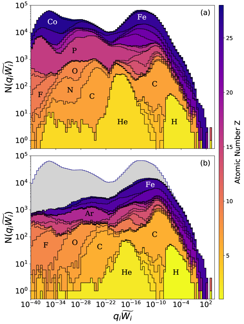
Figure 3: Comparison of the contributions by element to the total distribution of line strengths. (a) shows all transitions, including theoretical. (b) excludes theoretical transitions from the CMFGEN and CHIANTI databases. Major element contributions labeled, for example temperature $T=5200$ K and density $\rho=10^{-13}$ g cm^-3. In (b) grey indicates contour of the total histogram from (a).

4 Calculating and Fitting the Line Force Multiplier

In order to examine the dynamics of the outflows, we first calculate the line force multiplier, a measure of the strength of the radiation force, from our updated list of spectral lines and distributions of $q_{i}\widetilde{W}_{i}$. We then fit and compare two functions to the resulting distributions.

4.1 Calculating $M(t)$

The line acceleration is defined as the radiative acceleration due to electron scattering, multiplied by the line force multiplier $M(t)$. Here, $t$ is an optical depth parameter that is independent of the line strength. It is given by

$$t=\kappa_{e}\rho v_{\rm th}\left|\frac{dv}{dr}\right|^{-1}$$ (33)

for expanding atmospheres (Sobolev, 1957, 1960, CAK). In the case of a static atmosphere, $t$ is equivalent to the electron scattering optical depth, while in the expanding case $t$ is less than this depth.

In an expanding wind, we cannot simply take the sum of the $q_{i}\widetilde{W_{i}}=g_{\rm bound}/g_{\rm free}$ as found in Equation (15) above. The full force multiplier depends on other radiative transfer effects, such as the “self-shadowing” of the lines, due to differences in the Doppler-shifted local reference frames (Gayley, 1995). Therefore the full calculation of the force multiplier $M(t)$ from the line list can be written as

$$M(t)\,=\,\eta\,\sum_{i}q_{i}\widetilde{W}_{i}\left(\frac{1-e^{-\tau_{i}}}{\tau_{i}}\right)$$ (34)

where the geometrical finite-disk factor $\eta$ is the ratio of the true line force to that derived in the limit of purely radial photons (e.g., it is the same as the ratio $F$ given by Equation (21) of Gayley 1995). Equation (34) assumes the Sobolev approximation and no overlapping lines, for supersonic flows. The dimensionless optical depth $\tau_{i}$ of each line is defined as

$$\tau_{i}=\frac{c}{v_{\rm th}}q_{i}t$$ (35)

where $v_{\rm th}^{2}=2k_{\rm B}T/m_{p}$ is the proton thermal speed for all ions of a single temperature.

$M(t)$ corresponds to the sum over the spectral lines that contribute to the wind. Originally, $M(t)$ was parameterized by Castor (1974) in terms of the optical depth, depending only on the structure of the wind. However, CAK proposed that $M(t)$ could take the form of a power-law, expressed as

$$M(t)\,=\,\eta\,kt^{-\alpha}$$ (36)

where $k$ and $\alpha$ are the fit constants of the power-law. Because the finite disk factor $\eta$ appears in both Equations (34) and (36), we can safely neglect it when performing fits and parameterizations for quantities such as $k$ and $\alpha$. We re-examine the assumption presented in Equation (36) that the line force multiplier takes the form of a power law. To do this, we will fit both power laws and an alternative fitting function to the values of $M(t)$ calculated from the updated line list.

Although the CAK $t$ parameter can be evaluated at any point in a radiatively-driven outflow, here we evaluate $M(t)$ over a logarithmic grid of $t$ spanning from $10^{-15}$ to $10$. In the limit of $t\rightarrow 0$ the line-force multiplier $M(t)$ should become equal to $\bar{Q}$. It should be noted that Abbott (1982) considers only values of $t$ from $10^{-7}$ to $t=0.1$. However, we include values beyond this range in order to better examine the behavior of $M(t)$. For example, the asymptotic behavior of $M(t)$ in the limit of small $t$ is not seen in the range used by Abbott (1982).

In calculating the dimensionless line strength parameter $q_{i}$, the weighting function $\widetilde{W_{i}}$, and subsequently the force multiplier $M(t)$ as described above, we used a grid of 100 logarithmically spaced temperatures ranging from 5,200 to 70,000 K and 22 densities ranging from $10^{-20}$ to $10^{-10}$ g cm^-3. We calculated the force multiplier $M(t)$ for two cases: (1) the full line list that includes both observed and theoretical lines, and (2) only the subset of observed lines with laboratory wavelengths. Figure 4 shows results for $M(t)$ for both cases. In general, note that both higher temperatures and higher densities tend to result in higher values of the force multiplier. Note also that the turnover to a constant value of $M(t)\approx\bar{Q}$ occurs at different values of $t$; this is sometimes as low as $t\approx 10^{-10}$ and sometimes as high as $t\approx 10^{-4}$. Stevens & Kallman (1990) calculated the radiative force due to X-ray ionization on the stellar wind in massive X-ray binaries. The flattening of the $M(t)$ curve seen in Figure 4 is similar to Figure 1 of that paper, where the force multiplier is suppressed with increasing X-ray ionization.

Figure 5 shows the ratio of the full and observed-only calculations for an example value of $t\approx 1$. The discrepancy between the two multipliers is most pronounced at high temperatures, with the full line list producing a much higher force multiplier than the observed-only list. This is to be expected, as the observed-only list does not include many lines from high-$Z$ elements which require high temperatures to ionize. However, at lower temperatures the discrepancy between the two calculations is slight. In light of these factors, going forward we use only the full line list that includes theoretical lines.

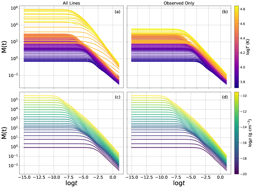
Figure 4: The force multiplier $M(t)$: (a) Varying with temperature from $T=$5,200 K to $T=$70,000 K for a constant density of $\rho=10^{-20}$ g cm^-3, for observed and theoretical transitions. (b) Varying with temperature from $T=$5,200 K to $T=$70,000 K for a constant density of $\rho=10^{-20}$ g cm^-3, for only observed transitions. (c) Varying with density from $\rho=10^{-20}$ g cm^-3 to $\rho=10^{-10}$ g cm^-3 for a constant temperature of $T=5,200$ K, for theoretical and observed transitions. (d) Varying with density from $\rho=10^{-20}$ g cm^-3 to $\rho=10^{-10}$ g cm^-3 for a constant temperature of $T=5,200$ K, for only observed transitions.

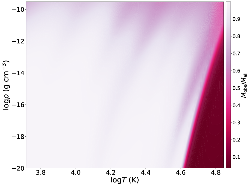
Figure 5: Ratio of the calculated force multiplier for line lists comprised of all lines to observed lines only, shown here for an example value of $t\approx 1$.

Figure 6 shows the sum $\bar{Q}=\sum_{i}q_{i}\widetilde{W_{i}}$, which was calculated for each temperature and density. These are compared to values from Gayley (1995), who also provided values of $\bar{Q}$ as converted from previous works such as Abbott (1982). Note that temperatures corresponding to O and early-B spectral types ($\log T$ between 4.2 and 4.6) tend to exhibit values of $\bar{Q}$ around $10^{3}$, independent of density, as also found by Gayley (1995). Above and below this range, there is a strong dependence of $\bar{Q}$ on density, with $\bar{Q}$ varying drastically at both very low temperatures ($\log T\lesssim 4.0$), and very high temperatures ($\log T\gtrsim 4.7$). This probably indicates that departures from LTE Saha ionization balance are more important to take into account for these temperatures.

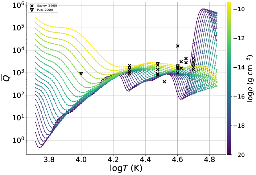
Figure 6: Evolution of $\bar{Q}$ for our chosen density and temperature range, compared to values from Table 1 of Gayley (1995) (black crosses) and Table 2 of Puls et al. (2000) (black triangles).

4.2 CAK Power Law Fitting

We begin by fitting a power law of the form proposed by CAK (Equation (36)) to the calculated values of $M(t)$. This fitting was performed using the Levenberg-Marquardt method of least-squares fitting. As is readily apparent from Figure 4, the full range of calculated $M(t)$ values cannot be described by a single power law. Therefore, we fit the initial CAK power law form to only to values of $\log(t)>-3$, in order to exclude the flat portion of the curve.

As with $\bar{Q}$, we also compare the fitted values of $\alpha$ and $k$ to those from previous work. Figure 7 shows a comparison to Abbott (1982), Shimada et al. (1994), Gayley (1995), and Gormaz-Matamala et al. (2019), with a good agreement with those values, most especially for densities that fall in the middle of our considered density range. Note that for the lowest values of $T$, our values for the power-law slope $\alpha$ never get as small as some of the plotted literature values that are of order $\sim$0.45. This may be explained if the power-law fits performed in other papers included portions of the flattened parts of $M(t)$. For example, Abbott (1982) calculated values of $\alpha$ and $k$ for a range of $-6\leq\log(t)\geq-1$ for a density grid similar to our own. We find that for low temperatures, the flat portions of the $M(t)$ curve begin at values of $t$ as high as $\log(t)\sim-2.5$. Inclusion of these flat portions during fitting would yield shallower slopes than those found in this work.

Despite acceptable agreement with previous works for these two parameters ($\alpha$, $k$), this preliminary power law form of the force multiplier presents a decent fit to the calculated values of $M(t)$ for only a narrow range of $t$, namely between $\log(t)\approx-3$ and $\log(t)\approx 0$.

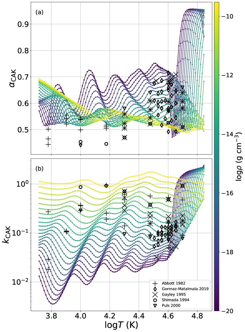
Figure 7: Comparison of CAK power law parameters $\alpha$ (a) and $k$ (b) with values from Abbott (1982), Shimada et al. (1994), Gayley (1995), Puls et al. (2000), and Gormaz-Matamala et al. (2019), for the our chosen range of densities.

4.3 Alternate Fitting Function

We present an alternative fitting function in the form of a saturated power law, given by

$$M(t)=\frac{\eta\bar{Q}k}{(k^{s}+\bar{Q}^{s}t^{\alpha s})^{1/s}}.$$ (37)

In this case, $\alpha$, $k$, and $s$ are fit parameters, and $\bar{Q}$ is the calculated value as found from the line list and shown in Figure 6. The parameter $s$ is a sharpness parameter that determines how rapidly the function transitions from the low-$t$ to high-$t$ limits. This function reduces to the CAK power law form in the limit of large $t$, and in the limit of small $t$ reduces to $\bar{Q}$, consistent with the behavior of the calculated values of $M(t)$. Figure 8 shows the resulting fits compared to the calculated $M(t)$ values, for an example density of $\rho=10^{-20}$ g cm^-3. The above function was found to be flexible enough to fit the calculated $M(t)$ values quite accurately. For the full grid of parameters ($T$, $\rho$, and $t$) we computed the fractional difference $D$ between the numerical and best-fit values of $M(t)$. The median of this distribution was $\langle D\rangle=1.95$%, and only a tiny fraction of the model values (1.03%) had values of $D>30$%.

The fits of the alternative function and the CAK power law are comparable for values of $\log t\gtrsim-4$. However, for values of $\log t\lesssim-4$, the fit achieved using the alternate function is drastically improved over that of the CAK power law. As can be seen in Figure 4, the value of $t$ at which the CAK power law begins to fail also strongly depends on temperature and density. Additionally, we do not include a high opacity cut-off in our new form of $M(t)$, such as that suggested by Gayley (1995). Upon calculation of the force multiplier out to high $t$ ($t\sim 10^{15}$), we find that $M(t)$ continues to decrease as a power-law rather than as an exponential drop-off at high opacities, generally approaching the form $M(t)\propto t^{-1}$ as temperature and density increase. Therefore, we do not impose a cut-off of the force multiplier at high opacities.

Figure 9 shows the dependence of the saturated power law fit parameters $\alpha$, $k$, and $s$ on temperature and density. Also shown is the evolution with temperature and density of $M(t)$ at $t=1$. At high values of $t$ such as $t=1$, the force multiplier behaves as a power-law. The values of $M(t=1)$ provide an alternate estimation of the fit parameter $k$. Comparison of Figures 9(a) and 9(b) additionally provide insight into the deviation of the fitted saturated power-law (a) from the actual calculated value (b). We also include an estimate of the CAK critical point density across the range of effective temperatures (see Section 5.4). Additionally, we indicate a locus of parameters at which the Saha ionization balance produces equal amounts of Fe III and Fe IV. The relevance of this to a proposed explanation for the phenomenon of “bistability” in line-driven winds is discussed further in Section 6.

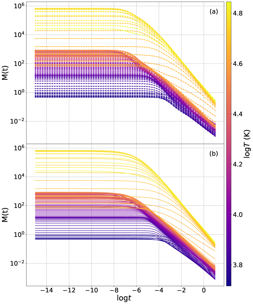
Figure 8: Comparison of alternate fits and calculated values of M(t) for an example density of $\rho=10^{-20}$ g cm^-3. (a) $M(t)$ as calculated from line list. (b) Fits produced by Equation (37).

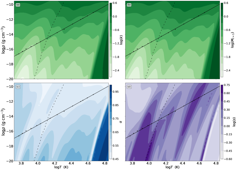
Figure 9: Two-dimensional contour plots of the temperature and density dependence of the fit parameters for the alternate fitting function. (a) $k$, (b) $M(t=1)$, (c) $\alpha$, (d) $s$. Solid lines indicate estimates of the density at the CAK critical point (Equation (56)), and dashed lines indicate the calculated recombination temperature of Fe between Fe III and Fe IV.

5 Mass-Loss Estimates for Massive Stars

In addition to determining a function to better describe the line force multiplier $M(t)$, we also explore the consequences of this updated form on the calculated mass-loss rates of massive stars. We do this by calculating mass-loss rates for both the traditional power-law form and our newly updated alternate form.

5.1 General Mass-Loss Solution

We begin with the time-steady radial component of the momentum conservation equation. To approximate the supersonic winds of OB stars, we omit the gas-pressure gradient term. Because gas pressure does not play a fundamental role in highly supersonic winds such as the ones considered in this work, we can safely neglect these terms (see, e.g., Gayley, 2000; Owocki, 2004). Doing this, we have

$$v\frac{\partial v}{\partial r}=-\frac{GM_{*}}{r^{2}}+g_{\rm free}+g_{\rm bound}.$$ (38)

Here, $v(r)$ is the radially dependent wind velocity, $M_{*}$ is the mass of the central star, and $G$ is the gravitational constant. The free radiative acceleration due to Thomson scattering $g_{\rm free}$ can be written as the Eddington factor $\Gamma$ times the gravitational acceleration. With stellar bolometric luminosity $L_{*}$, the Eddington factor $\Gamma$ can be written as

$$\Gamma=\frac{\kappa_{e}L_{*}}{4\pi cGM_{*}}$$ (39)

with the mixture-dependent Thomson scattering coefficient given by

$$\kappa_{e}\,=\,\frac{\sigma_{T}n_{e}}{\rho}\,\approx\,\frac{\sigma_{T}}{m_{H}}\left(\frac{1+X}{2}\right)$$ (40)

where $X$ is the hydrogen mass fraction. The final approximation above is provided only for reference in the limit of full ionization (see, e.g., Mihalas, 1978). In all results shown below, we use the self-consistent values of $n_{e}$ computed from the Saha equation. For the values of $X$ and $Y$, we use the bulk composition chemical abundances of H and He given in Table 4 of Asplund et al. (2009), with $X=0.7154$ and $Y=0.2703$. Using Equations (38)–(40), we can write the equation of motion as

$$v\frac{\partial v}{\partial r}=\frac{GM_{*}}{r^{2}}\left[-1+\Gamma+\Gamma M(t)\right].$$ (41)

As in Gayley (1995), we also define the dimensionless wind acceleration factor $w$:

$$w=\frac{r^{2}v}{GM_{*}(1-\Gamma)}\frac{dv}{dr}.$$ (42)

This allows us to write Equation (41) as

$$F_{1}=w+1-\frac{\Gamma}{1-\Gamma}M(t)=0.$$ (43)

We use this form because the CAK critical-point solution requires at least two conditions to be true for a time-steady wind:

$$F_{1}=0\textrm{ and }F_{2}=\frac{\partial F_{1}}{\partial w}=0.$$ (44)

Using mass conservation, we can write the density as $\rho=\dot{M}/(4\pi r^{2}v)$. Combining the definitions of the CAK $t$ parameter and the wind acceleration factor $w$, as given in Equations (33) and (42) respectively, we can then write $t$ as $t=t_{m}/w$, where

$$t_{m}=\frac{v_{\rm th}c\dot{M}\Gamma}{L_{*}(1-\Gamma)}.$$ (45)

This is equivalent to Equation (52) of Gayley (1995). We now can solve Equation (44) for $w$ and $t_{m}$ to determine the mass-loss rate.

5.2 Mass-Loss Rates for the CAK Multiplier

We begin with the traditional CAK power-law form of the force multiplier as given in Equation 36, assuming that the parameters $\alpha$ and $k$ are known for a given set of lines. Extending beyond CAK, we also include the finite disk factor $\eta$, which has a simple form for a CAK-like force multiplier when evaluated at the stellar surface:

$$\eta\approx\frac{1}{1+\alpha}$$ (46)

(Kudritzki et al., 1989). Therefore we can write the critical point conditions $F_{1}$ and $F_{2}$ as

$$F_{1}=w+1-Cw^{\alpha}=0$$ (47)

$$F_{2}=1-\alpha Cw^{\alpha-1}=0$$ (48)

where $C=\eta\Gamma k(1-\Gamma)^{-1}t_{m}^{-\alpha}$. Solving $F_{2}$ for $C$ and re-solving $F_{1}$ for $w$, we find the analytic solutions

$$w=\frac{\alpha}{1-\alpha}\textrm{ and }C=\frac{1}{\alpha^{\alpha}(1-\alpha)^{1-\alpha}}.$$ (49)

Using this solution for $C$, we can solve for $t_{m}$, which can then be converted to $\dot{M}_{\rm CAK}$. Combining equations (47)–(49) and recalling the definition of $t_{m}$ from Equation (33), we find the mass-loss rate $\dot{M}_{\rm CAK}$:

$$\dot{M}_{\rm CAK}=\frac{L_{*}(1-\Gamma)}{v_{\rm th}c\Gamma}\left[\frac{\alpha^{\alpha}\eta\Gamma k(1-\alpha)^{1-\alpha}}{(1-\Gamma)}\right]^{1/\alpha}.$$ (50)

It is worth mentioning here that the apparent dependence of $\dot{M}_{CAK}$ on the Doppler thermal width $v_{\rm th}$ is in fact only a fiducial dependence, due to the definition of the $t$ parameter (Equation (33)), which introduces $v_{\rm th}$ and is subsequently present in Equation (45). While a reformulation of $t$ could eliminate this dependence, we choose to carry it through our calculations in order to maintain a level of comparability with previous works, notably that of CAK.

5.3 Mass-Loss Rates for Updated Formalism

Next, we solve the critical-point equations for our more general form of $M(t)$, given by Equation (37). Combining Equations (43) and (44), we find $F_{1}$ and $F_{2}$ are now given by

$$F_{1}=w+1-B\left[\frac{kw^{\alpha}}{(k^{s}w^{\alpha s}+\bar{Q}^{s}t_{m}^{\alpha s})^{\frac{1}{s}}}\right]=0$$ (51)

$$F_{2}=1-B\alpha\left[\frac{(kw^{\alpha-1})(\bar{Q}^{s}t_{m}^{\alpha s})}{(k^{s}w^{\alpha s}+\bar{Q}^{s}t_{m}^{\alpha s})^{\frac{1}{s}+1}}\right]=0$$ (52)

where $B=\eta\Gamma\bar{Q}/(1-\Gamma)$. Solving Equation (51) for

$$\bar{Q}^{s}t_{m}^{\alpha s}=\left(\frac{kw^{\alpha}B}{w+1}\right)^{s}-k^{s}w^{\alpha s},$$ (53)

we substitute the result into Equation (52). This gives

$$0=wB^{s}+\alpha(w+1)\left[(w+1)^{s}-B^{s}\right].$$ (54)

In the $\bar{Q}\rightarrow\infty$ ($B\gg 1$) limit, Equation (54) reduces to the CAK behavior, with a solution of $w=\alpha/(1-\alpha)$ as in Equation (49). In the opposite limit ($B\rightarrow 0$), the above equation is solved only by $w\approx-1$, which is unphysical (see below).

For the nominal case of $s=1$, Equation (54) reduces to a quadratic equation with two unique solutions for $w$:

$$w=-\frac{B(1-\alpha)}{2\alpha}-1\pm\frac{B(1-\alpha)}{2\alpha}\sqrt{1+\frac{4\alpha}{B(1-\alpha)^{2}}}$$ (55)

However, in the more general case of $s\neq 1$ Equation (54) must be solved numerically. In this work this is done using the Newton-Raphson method. Once the acceleration factor $w$ is known, we can then find $t_{m}$ from Equation (53), which then in turn allows us to find the mass-loss rate $\dot{M}_{\rm alt}$ from Equation (45).

It is relevant to note that in calculating the mass-loss rates that result from both the CAK and alternate forms, we discard any sets of parameters that result in $\Gamma\geq 1$ (since we do not include multiple-scattering effects or super-Eddington flows). Similarly, we discard as unphysical any negative solutions of the wind acceleration factor $w$. In Equations (54) and (55) above, the condition $w\geq 0$ corresponds to $B\geq 1$. Since both $\eta$ and $(1-\Gamma)$ tend to be order-unity quantities, the condition for physically realistic solutions is thus $\Gamma\gtrsim\bar{Q}^{-1}$. With typical values of $\bar{Q}$ of a few thousand, this implies that whenever $\Gamma$ drops below $\sim 10^{-3}$, a steady-state line-driven wind may not be possible.

5.4 CAK Critical Point and Stellar Parameters

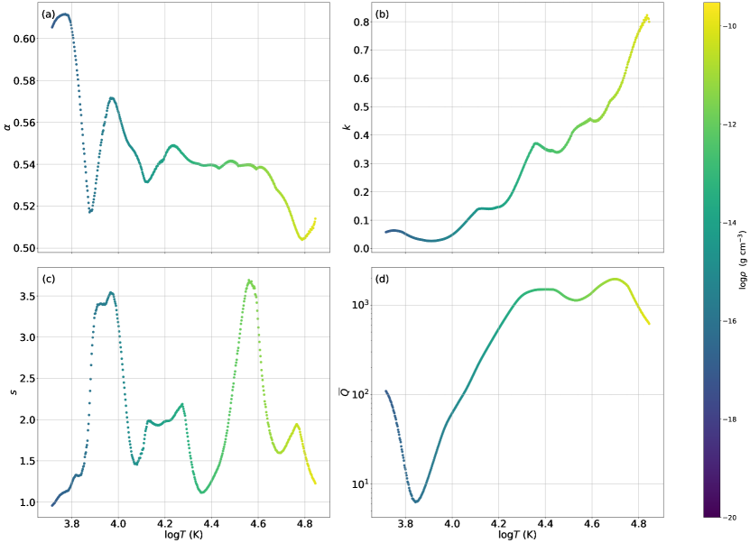
Figure 10: Evolution with temperature of the four parameters that define the saturated power-law form of $M(t)$ along the CAK critical point line. (a) $\alpha$, (b) $k$, (c) $s$, (d) $\bar{Q}$.

Although the force multiplier $M(t)$ is a function of both $T$ and $\rho$, it is possible to characterize much of the physics by evaluating $M(t)$ at the critical point of the flow (see, e.g., CAK; Abbott, 1980; Pauldrach et al., 1986; Bjorkman, 1995). To do this, we need to know both the temperature and the density at the critical point. For an isothermal wind, $T$ at the critical point is given more or less by the photospheric effective temperature. The only way to estimate the density $\rho_{\rm crit}$ at the critical point, though, is to have an associated “initial guess” for the full radial dependence of the plasma parameters. We provide this initial guess for a set of idealized main-sequence stellar properties (see Section 5.5) by using a modified-CAK (mCAK) numerical code developed by Cranmer & Owocki (1995). This code solves the equations of mass and momentum conservation for the power-law CAK force multiplier and a standard version of the uniformly illuminated finite-disk factor $\eta$. When considering finite sound-speed effects, it is necessary to solve simultaneous singularity and regularity conditions for the properties of the critical point (CAK).

For a sequence of stellar properties spanning effective temperatures between 5,920 and 46,000 K (see below for details), we produced mCAK models with fixed line-force constants $\alpha=0.6$ and $k=0.5$. These models all exhibited critical points at radial distances between 1.01 and 1.02 times the photospheric stellar radius, critical wind speeds between about 50 and 120 km s^-1 (i.e., typically about 3% of the asymptotic or terminal wind speeds of 2,000–3,000 km s^-1), and values of $\rho_{\rm crit}$ between $10^{-17}$ and $10^{-11}$ g cm^-3. Figure 9 shows this trend in two-dimensional ($T$, $\rho$) diagrams. A power law of the form

$$\rho_{\rm crit}=\left(6.33\times 10^{-16}\textrm{ g~{}cm}^{-3}\right)\left(\frac{T}{10^{4}\textrm{ K}}\right)^{6.2}$$ (56)

is reasonably successful at capturing this trend as well. Figure 10 shows how the calculated parameter $\bar{Q}$ and the fit parameters $\alpha$, $k$, and $s$ vary with temperature along the CAK critical point curve, which corresponds to the black dashed line shown in Figure 9.

For the remainder of this work we use the stellar color and effective temperature sequence as in Table 5 of Pecaut & Mamajek (2013) to calculate mass-loss rates using the methods described in above. Figure 11 shows the continuous functions fit to the data from this table for both temperature-luminosity and temperature-mass relationships. These take the the form of a power-law and a third order polynomial respectively, given by

$$\log(L/L_{\odot})=6.73\log(T)-25.47$$ (57)

and

$$\log(M/M_{\odot})=1.29\log(T)^{3}-15.44\log(T)^{2}\\ +63.02\log(T)-87.23.$$ (58)

For the purposes of this work, we assume that the wind temperature $T$ in K remains equal to the stellar effective temperature $T_{\rm eff}$. These fits were done so that mass and luminosity could be calculated for any temperature along our temperature range. These fits were only calculated for the range of data that our temperature range encompasses in order to disregard behavior at the low temperature end of the main sequence.

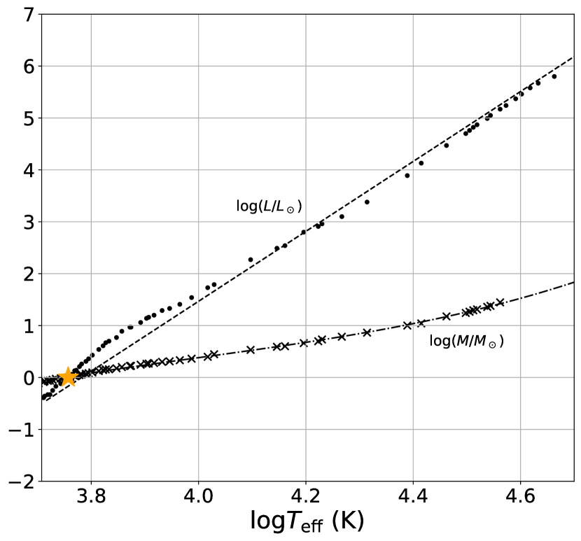
Figure 11: Main-sequence stellar parameters from Pecaut & Mamajek (2013). Black points indicate temperature-luminosity relationship, black crosses indicate temperature-mass relationship. Functions fitted to the data points are indicated by dashed and dot-dashed lines respectively. Orange star indicates the location of the Sun.

5.5 Comparison of Mass-Loss Rates

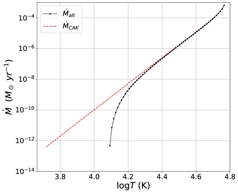
Figure 12: Preliminary comparison of $\dot{M}_{\rm CAK}$ and $\dot{M}_{\rm alt}$ for $\alpha=0.7$, $k=0.5$, and $\bar{Q}=2000$. Red dashed line indicates $\dot{M}_{\rm CAK}$.

Figure 12 shows a preliminary comparison of $\dot{M}_{\rm CAK}$ and $\dot{M}_{\rm alt}$. We hold steady the parameters $\bar{Q}$, $\alpha$, $k$, and $s$, with only temperature $T$ varying, and mass and luminosity dependent on temperature as described above. There is good agreement between $\dot{M}_{\rm CAK}$ and $\dot{M}_{\rm alt}$ at high temperatures. However, there is a steep drop off exhibited at $\sim 12,000$K in $\dot{M}_{\rm alt}$, whereas $\dot{M}_{\rm CAK}$ continues as a power-law described by

$$\dot{M}_{\rm CAK}\propto T^{8.51}.$$ (59)

Using Equation (57), this can also be written as

$$\dot{M}_{\rm CAK}\propto\left(\frac{L_{\ast}}{L_{\odot}}\right)^{1.26}.$$ (60)

This is in comparison to the common form $\dot{M}\propto L_{\ast}^{1/\alpha}$. For a value of $\alpha=0.7$ as in Figure 12, this would take the form $\dot{M}\propto L_{\ast}^{1.42}$, whereas Equation (60) shows a slightly weaker dependence on luminosity. In Figure 12, the black curve for $\dot{M}_{\rm alt}$ shows a strong drop-off, or quenching, which is a result of the flattening of the force multiplier at low values of $t$.

Next we introduce varying values of $\alpha$, $k$, $\bar{Q}$ and $s$. These parameters vary according to temperature and density, as seen in Section 4.3. For the remainder of this work we consider only the version of $\dot{M}_{\rm alt}$ in which all four parameters ($\alpha$, $k$, $\bar{Q}$, $s$) are allowed to vary with temperature and density. Figure 13 shows the variations of $\dot{M}_{\rm alt}$ with $T$ and $\rho$.

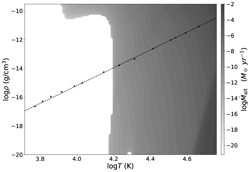
Figure 13: Contours of $\dot{M}_{\rm alt}$ over density and temperature. Dashed line indicates the CAK critical point density.

Figure 14 compares the mass-loss rates resulting from the CAK and alternate form. As in Figure 12, we see a sharp drop-off of $\dot{M}_{\rm alt}$ in comparison to the CAK form, commonly occurring at $\log T\approx 4.2$. At high densities ($\rho>10^{-11}$ g cm^-3) the departure from the CAK form is less pronounced, although still present. It should be noted that in these figures the apparent plotted end of $\dot{M}_{\rm alt}$ between $10,000$ and $20,000$ K is a result of discarding any wind solution that results in a negative wind acceleration factor $w$. Physically, this represents regions of the parameter space where the wind is quenched, a phenomenon that is not evident when $M(t)$ is modeled as a pure power-law function of $t$.

Also shown in Figure 14 is the photon-tiring limit, which constrains the maximum possible mass-loss rate $\dot{M}_{\rm max}$ (Owocki & Gayley, 1997). This is limit is defined by when the kinetic energy carried away by the wind is equal to the photon energy carried by the stellar luminosity, and is also dependent on the terminal velocity of the wind. If the terminal velocity $v_{\infty}$ is defined as $v_{\infty}=fv_{\rm esc}$, then the limit $\dot{M}_{\rm max}$ is given by

$$\dot{M}_{\rm max}=\frac{2}{f^{2}}\frac{L_{\ast}}{v_{\rm esc}^{2}},$$ (61)

with the escape velocity given by $v_{\rm esc}^{2}=2GM_{\ast}/R_{\ast}$. For this work we take the traditional value of $f=3$. For lower densities ($\rho\lesssim 10^{-16}$ g/cm^-3), we see that the photon-tiring limit intersects the mass-loss rate curves at approximately the same point at high temperatures where $\Gamma\geq 1$.

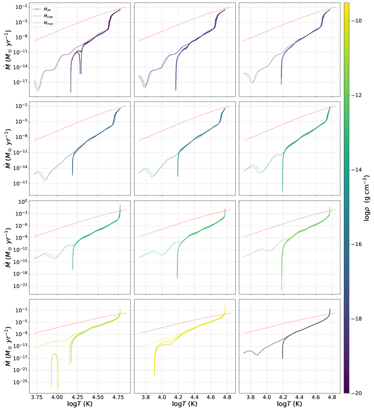
Figure 14: Comparison of $\dot{M}_{\rm CAK}$ and $\dot{M}_{\rm alt}$, by density order of magnitude. Dashed lines indicate $\dot{M}_{\rm CAK}$, solid lines indicate $\dot{M}_{\rm alt}$. Lower right corner shows calculations of $\dot{M}_{\rm CAK}$ and $\dot{M}_{\rm alt}$ for the calculated critical point densities. Red dashed lines indicate the photon-tiring limit.

6 Discussion and Conclusions

In this work, we have constructed an updated list of atomic data, with data for 4,514,900 spectral lines taken from the NIST, CMFGEN, CHIANTI, and TOPbase databases. These atomic data were then used to calculate the line strength parameter $q_{i}$ for each line for a density range of $10^{-20}$ to $10^{-10}$ g cm^-3 over a temperature range of 5,200 to 70,000 K. The weighting function $\widetilde{W_{i}}$ was also calculated. These parameters were used to find the line force multiplier $M(t)$ over a range of $t$ from $10^{-15}$ to $10$. The distribution of $M(t)$ was fit using a power-law as described by Equation (36), as well as an alternate function in the form of a saturated power-law, as described by Equation (37). We found that this alternative function better describes the values of the line-force multiplier as calculated from the updated line list, especially at low values of $t$. The residuals of this alternate function are consistently lower than those that result from the CAK form in the case of low $t$, and comparable for high values of $t$. This is consistent across temperatures and densities. We include the parameter $s$ to control the sharpness of the turn-over from the power-law segment to the flat segment. $M_{\rm alt}(t)$ reduces to the power-law form in the limit of high-$t$ for all values of the sharpness parameter s. In the limit of low-$t$ $M_{\rm alt}(t)$ similarly reduces to the calculated value of $\bar{Q}$.

Using the alternate function for $M(t)$, we also calculate mass-loss rates for the temperatures and densities in our grid, using the fitted parameters $\alpha,k,\textrm{ and }s$, along with the corresponding calculated values of $\bar{Q}$. We find that the sharpness parameter $s$ has a drastic effect on the determined mass-loss rates, especially at high temperatures. Additionally, there is a sharp drop-off in the mass-loss rates calculated from the updated form of $M(t)$ and a resulting discrepancy between it and the CAK mass-loss form. This drop-off in the mass-loss rate describes a quenching of the line-driven wind that is not present in the CAK form.

We find that the quenching of the wind typically occurs between temperatures of $10,000$ K and $20,000$ K and at luminosities of ${2.5}\lesssim\log(L_{*}/L_{\odot})\lesssim{2.75}$. This may be a partial explanation for the discrepancy noted between empirically derived mass-loss rates and predicted values for stars of luminosities below $\sim 10^{5}\,L_{\odot}$ ($T\approx 36,000$ K), often referred to in the literature as the “weak-wind problem” (Muijres et al., 2012), although it should be noted that our calculations place the quenching of the wind at lower luminosities and temperatures. It is also possible that these effects could be important to include when modeling the oscillations of Slowly Pulsating B (SPB) stars, which have $T_{\rm eff}$ values between about 10,000 and 20,000 K (De Cat, 2007). The interactions between their oscillations and winds remain poorly understood (e.g., Saio, 2015).

Lastly, there is another physical effect that must be taken into account to fully understand how the predicted quenching effect manifests itself: collisionless decoupling between the line-driven ions and the dominant hydrogen/helium gas. This has been proposed to be important both for B-type stars (Springmann & Pauldrach, 1992; Babel, 1996; Krtička, 2014) and some metal-enriched AGNs (Baskin & Laor, 2012). In some low-density systems this decoupling can lead to frictional heating with wind temperatures far in excess of the stellar $T_{\rm eff}$, and in others may produce fully-separated multi-component winds with peculiar chemical abundances. It may be possible that the drastic reduction in the ion line-force (which arises due to the flattening of the force multiplier) allows these systems to undergo a more gentle and gradual transition from a coupled single-fluid outflow to a quiescent hydrostatic atmosphere.

Although here we consider only the assumption of LTE, other similar works consider the effects of NLTE (see, for example, Gormaz-Matamala et al., 2019). Puls et al. (2000) accounted for NLTE effects in the line distribution by restricting the types of lines used to those with or directly connected to those with a ground or metastable lower level. For our purposes, it will be useful to refine the ionization balance used here using the modified nebular approach described by others (see, for example, Abbott & Lucy, 1985, Gormaz-Matamala et al., 2019). Although the assumption of a Planck function for $F(\nu)$ allowed us to maintain generality in this work, in future work it will be necessary to refine our choice of $F(\nu)$ to a more realistic distribution. For example, a self-consistent treatment of absorption in the near-star atmosphere could be applied to the phenomenon of “bistability” (e.g Lamers & Pauldrach, 1991) in which the wind sees a lower flux shortward of 91.2 nm—and a higher flux in the Balmer continuum—and this affects the relative strengths of the lines that contribute to $M(t)$. Alternatively, this bistability jump could be a result of the recombination of Fe between Fe III and Fe IV, with the contribution of the Fe III lines dominating the radiative acceleration of the subsonic part of the wind (Vink et al., 1999; Vink, 2000). Puls et al. (2000) similarly found that at low line strengths mass-loss is dominated largely by the radiative acceleration of iron group elements, with lighter ions playing a more important role at larger line strength. This bistability jump is predicted to be reflected by an increase in mass loss, occurring around $\sim$20,000 K. Our calculations show that the relevant recombination temperature of Fe IV does occur at a local maximum of the CAK $k$ parameter (see Figure 9(a)). However, while the mass-loss rate is usually quite sensitive to $k$, we do not see any significant increase in our final calculations for $\dot{M}$ at these parameters (e.g., Figure 14).

In this study we have also limited ourselves to the solar elemental abundances of Asplund et al. (2009). Other abundance patterns, such as those found in nearby galaxies with lower metallicity (Puls et al., 1996) or in certain types of chemically peculiar stars (Alecian & Stift, 2019) should be explored. Additionally, we plan to explore the radial dependence of the $t$ parameter and the associated spatial variation of $M(t)$ in self-consistent models of radial outflow from stars and other luminous astrophysical sources such as active galactic nuclei.

Appendix A Database Selection and Specific Line Counts

In cases where more than one database listed atomic data for a given ion, the database with the largest number of available transitions was used for each ionization state of each element. In general, CMFGEN was found to contain the most lines for a majority of ions. However, where CMFGEN data was nonexistent or insufficient, the database with the next most lines was used. Generally, this was CHIANTI. For several elements and ionization states (namely N VI, N VII, Cl VIII, Cl IX, and Ni X), the necessary atomic data was not available from the databases used. Table 1 shows a breakdown of line counts $n$ by ion, with the database used for each also listed. In some databases, transitions with a both a radiative decay rate and an autoionization rate were represented twice. After compiling the line list from the total available data, we discarded any such duplicate transitions.

Table 1: Number of lines ($n$) and database used for each ion. A dash (-) indicates that no data were available. CMFGEN, NIST, CHIANTI, and TOPbase are abbreviated as CM, N, CH, and T respectively.

Ion	$n$	Database	Ion	$n$	Database	Ion	$n$	Database	Ion	$n$	Database
H I	435	CM	Na V	10644	CM	Cl IV	8612	CM	V III	21	N
He I	3857	CM	Na VI	10994	CM	Cl V	3388	CM	V IV	239	N
He II	435	CM	Na VII	5436	CM	Cl VI	2377	CM	V V	10	N
Li I	68	N	Na VIII	4742	CM	Cl VII	1557	CM	V VI	4	N
Li II	134	N	Na IX	4201	CH	Cl VIII	-	-	V VII	7	N
Li III	2	N	Na X	331	CH	Cl IX	-	-	V VIII	6	N
Be I	175	N	Mg I	2841	CM	Cl X	24	CH	V IX	16	N
Be II	97	N	Mg II	2641	CH	Ar I	3824	CM	V X	13	N
Be III	100	N	Mg III	4753	CH	Ar II	79388	CM	Cr I	49885	CM
Be IV	10	N	Mg IV	5706	CM	Ar III	6901	CM	Cr II	66400	CM
B I	96	N	Mg V	6377	CM	Ar IV	11290	CM	Cr III	-	-
B II	150	N	Mg VI	14480	CM	Ar V	8350	CM	Cr IV	67061	CM
B III	74	N	Mg VII	11940	CM	Ar VI	5	N	Cr V	43860	CM
B IV	134	N	Mg VIII	5820	CM	Ar VII	35	CH	Cr VI	4406	CM
B V	58	N	Mg IX	5517	CM	Ar VIII	2743	CH	Cr VII	46	CH
C I	10204	CM	Mg X	26078	CH	Ar IX	5691	CH	Cr VIII	131	CH
C II	8017	CM	Al I	4985	CM	Ar X	4435	CH	Cr IX	236	CH
C III	9468	CM	Al II	2870	CM	K I	1471	CM	Cr X	16	N
C IV	1297	CM	Al III	2665	CM	K II	38603	CM	Mn I	164	N
C V	2196	CM	Al IV	5296	CH	K III	220	CM	Mn II	49066	CM
C VI	1575	CM	Al V	6607	CH	K IV	18227	CM	Mn III	70218	CM
N I	855	CM	Al VI	7989	CM	K V	7252	CM	Mn IV	72374	CM
N II	7879	CM	Al VII	15486	CM	K VI	14870	CM	Mn V	77009	CM
N III	6710	CM	Al VIII	13501	CM	K VII	71	N	Mn VI	70116	CM
N IV	13886	CM	Al IX	5859	CM	K VIII	95	N	Mn VII	8277	CM
N V	1296	CM	Al X	5041	CM	K IX	2758	CH	Mn VIII	47	CH
N VI	2263	CM	Si I	2791	CM	K X	5700	CH	Mn IX	137	CH
N VII	3150	CM	Si II	4196	CM	Ca I	106	N	Mn X	236	CH
O I	4145	CM	Si III	1328	CM	Ca II	238	CH	Fe I	141928	CM
O II	17874	CM	Si IV	2672	CH	Ca III	520	N	Fe II	530827	CM
O III	6516	CM	Si V	5354	CH	Ca IV	2	N	Fe III	136060	CM
O IV	7599	CM	Si VI	6518	CM	Ca V	9	CH	Fe IV	72223	CM
O V	3237	CM	Si VII	9364	CM	Ca VI	10	CH	Fe V	71983	CM
O VI	1569	CM	Si VIII	705	CH	Ca VII	86	CH	Fe VI	185392	CM
O VII	3505	CM	Si IX	403	CH	Ca VIII	200	CH	Fe VII	86504	CM
O VIII	1575	CM	Si X	5017	CH	Ca IX	9230	CH	Fe VIII	21134	CH
F I	119	N	P I	46	N	Ca X	2760	CH	Fe IX	47085	CH
F II	2354	CM	P II	217043	CM	Sc I	259	N	Fe X	50854	CM
F III	9725	CM	P III	5576	CM	Sc II	77253	CM	Co I	118	N
F IV	15	N	P IV	2537	CM	Sc III	687	CM	Co II	61986	CM
F V	11	N	P V	2700	CH	Sc IV	4	N	Co III	679412	CM
F VI	8415	T	P VI	5533	CH	Sc V	4	N	Co IV	69425	CM
F VII	6406	T	P VII	3	CH	Sc VI	-	-	Co V	75923	CM
F VIII	5614	T	P VIII	25	CH	Sc VII	15	N	Co VI	75118	CM
F IX	3488	T	P IX	59	CH	Sc VIII	16	N	Co VII	68388	CM
Ne I	2629	CM	P X	78	CH	Sc IX	15	N	Co VIII	88548	CM
Ne II	5795	CM	S I	19813	CM	Sc X	-	-	Co IX	12232	CM
Ne III	2343	CM	S II	8527	CM	Ti I	490	N	Co X	5	N
Ne IV	9725	CM	S III	4543	CM	Ti II	93118	CM	Ni I	188	N
Ne V	13037	CM	S IV	7530	CM	Ti III	21722	CM	Ni II	51812	CM
Ne VI	5171	CM	S V	3605	CM	Ti IV	1000	CM	Ni III	66511	CM
Ne VII	5213	CM	S VI	1936	CM	Ti V	4	N	Ni IV	72898	CM
Ne VIII	26832	CH	S VII	73	N	Ti VI	11	N	Ni V	75541	CM
Ne IX	216	CH	S VIII	54	N	Ti VII	1	N	Ni VI	79169	CM
Ne X	190	CH	S IX	51	N	Ti VIII	15	N	Ni VII	74411	CM
Na I	2778	CM	S X	57	N	Ti IX	14	N	Ni VIII	71614	CM
Na II	5054	CH	Cl I	75	N	Ti X	43	N	Ni IX	79227	CM
Na III	4368	CH	Cl II	52	N	V I	1095	N	Ni X	-	CM
Na IV	3754	CM	Cl III	50	N	V II	1415	N	-	-	-

References

- Abbott (1980) Abbott, D. C. 1980, ApJ, 242, 1183, doi: 10.1086/158550
- Abbott (1982) —. 1982, ApJ, 259, 282, doi: 10.1086/160166
- Abbott & Lucy (1985) Abbott, D. C., & Lucy, L. B. 1985, ApJ, 288, 679, doi: 10.1086/162834
- Alecian & Stift (2019) Alecian, G., & Stift, M. J. 2019, MNRAS, 482, 4519, doi: 10.1093/mnras/sty3003
- Asplund et al. (2009) Asplund, M., Grevesse, N., Sauval, A. J., & Scott, P. 2009, ARA&A, 47, 481, doi: 10.1146/annurev.astro.46.060407.145222
- Astropy Collaboration et al. (2013) Astropy Collaboration, Robitaille, T. P., Tollerud, E. J., et al. 2013, A&A, 558, A33, doi: 10.1051/0004-6361/201322068
- Babel (1996) Babel, J. 1996, A&A, 309, 867
- Baskin & Laor (2012) Baskin, A., & Laor, A. 2012, MNRAS, 426, 1144, doi: 10.1111/j.1365-2966.2012.21822.x
- Björklund et al. (2020) Björklund, R., Sundqvist, J. O., Puls, J., & Najarro, F. 2020, A&A, in press, arXiv:2008.06066. https://arxiv.org/abs/2008.06066
- Bjorkman (1995) Bjorkman, J. E. 1995, ApJ, 453, 369, doi: 10.1086/176396
- Cardona et al. (2010) Cardona, O., Martínez-Arroyo, M., & López-Castillo, M. A. 2010, ApJ, 711, 239, doi: 10.1088/0004-637X/711/1/239
- Cassinelli (1979) Cassinelli, J. P. 1979, ARA&A, 17, 275, doi: 10.1146/annurev.aa.17.090179.001423
- Castor et al. (1975) Castor, J. I., Abbott, D. C., & Klein, R. I. 1975, ApJ, 195, 157, doi: 10.1086/153315
- Castor (1974) Castor, J. L. 1974, MNRAS, 169, 279, doi: 10.1093/mnras/169.2.279
- Cranmer & Owocki (1995) Cranmer, S. R., & Owocki, S. P. 1995, ApJ, 440, 308, doi: 10.1086/175272
- Cunto & Mendoza (1992) Cunto, W., & Mendoza, C. 1992, Rev. Mexicana Astron. Astrofis., 23, 107
- Cunto et al. (1993) Cunto, W., Mendoza, C., Ochsenbein, F., & Zeippen, C. J. 1993, A&A, 275, L5
- De Cat (2007) De Cat, P. 2007, Communications in Asteroseismology, 150, 167, doi: 10.1553/cia150s167
- Dere et al. (2019) Dere, K. P., Del Zanna, G., Young, P. R., Landi, E., & Sutherland, R. S. 2019, ApJS, 241, 22, doi: 10.3847/1538-4365/ab05cf
- Dere et al. (1997) Dere, K. P., Landi, E., Mason, H. E., Monsignori Fossi, B. C., & Young, P. R. 1997, A&AS, 125, 149, doi: 10.1051/aas:1997368
- Drew (1989) Drew, J. E. 1989, ApJS, 71, 267, doi: 10.1086/191374
- Gayley (1995) Gayley, K. G. 1995, ApJ, 454, 410, doi: 10.1086/176492
- Gayley (2000) —. 2000, ApJ, 529, 1019, doi: 10.1086/308311
- Gormaz-Matamala et al. (2019) Gormaz-Matamala, A. C., Curé, M., Cidale, L. S., & Venero, R. O. J. 2019, ApJ, 873, 131, doi: 10.3847/1538-4357/ab05c4
- Higginbottom et al. (2014) Higginbottom, N., Proga, D., Knigge, C., et al. 2014, ApJ, 789, 19, doi: 10.1088/0004-637X/789/1/19
- Hillier (1990) Hillier, D. J. 1990, A&A, 231, 116
- Hillier & Lanz (2001) Hillier, D. J., & Lanz, T. 2001, in Astronomical Society of the Pacific Conference Series, Vol. 247, Spectroscopic Challenges of Photoionized Plasmas, ed. G. Ferland & D. W. Savin, 343
- Hillier & Miller (1998) Hillier, D. J., & Miller, D. L. 1998, ApJ, 496, 407, doi: 10.1086/305350
- Hubeny & Mihalas (2014) Hubeny, I., & Mihalas, D. 2014, Theory of Stellar Atmospheres
- Hunter (2007) Hunter, J. D. 2007, Computing in Science and Engineering, 9, 90, doi: 10.1109/MCSE.2007.55
- Johnson (1925) Johnson, M. C. 1925, MNRAS, 85, 813, doi: 10.1093/mnras/85.8.813
- Kee & Kuiper (2019) Kee, N. D., & Kuiper, R. 2019, MNRAS, 483, 4893, doi: 10.1093/mnras/sty3394
- Kee et al. (2018a) Kee, N. D., Owocki, S., & Kuiper, R. 2018a, MNRAS, 474, 847, doi: 10.1093/mnras/stx2772
- Kee et al. (2018b) —. 2018b, MNRAS, 479, 4633, doi: 10.1093/mnras/sty1721
- Kee et al. (2016) Kee, N. D., Owocki, S., & Sundqvist, J. O. 2016, MNRAS, 458, 2323, doi: 10.1093/mnras/stw471
- Kramida et al. (2018) Kramida, A., Yu. Ralchenko, Reader, J., & and NIST ASD Team. 2018, NIST Atomic Spectra Database (ver. 5.6.1), [Online]. Available: https://physics.nist.gov/asd [2019, September 11]. National Institute of Standards and Technology, Gaithersburg, MD.
- Krtička (2014) Krtička, J. 2014, A&A, 564, A70, doi: 10.1051/0004-6361/201321980
- Kudritzki et al. (1989) Kudritzki, R. P., Pauldrach, A., Puls, J., & Abbott, D. C. 1989, A&A, 219, 205
- Kudritzki & Puls (2000) Kudritzki, R.-P., & Puls, J. 2000, ARA&A, 38, 613, doi: 10.1146/annurev.astro.38.1.613
- Lamers & Pauldrach (1991) Lamers, H. J. G., & Pauldrach, A. W. A. 1991, A&A, 244, L5
- Lucy & Solomon (1970) Lucy, L. B., & Solomon, P. M. 1970, ApJ, 159, 879, doi: 10.1086/150365
- Mihalas (1978) Mihalas, D. 1978, Stellar Atmospheres, 2nd ed. (San Francisco: W. H. Freeman)
- Muijres et al. (2012) Muijres, L. E., Vink, J. S., de Koter, A., Müller, P. E., & Langer, N. 2012, A&A, 537, A37, doi: 10.1051/0004-6361/201015818
- Noebauer & Sim (2015) Noebauer, U. M., & Sim, S. A. 2015, MNRAS, 453, 3120, doi: 10.1093/mnras/stv1849
- Oliphant (2006) Oliphant, T. E. 2006, A guide to NumPy, Vol. 1 (Trelgol Publishing USA)
- Owocki (2004) Owocki, S. 2004, in EAS Publications Series, Vol. 13, EAS Publications Series, ed. M. Heydari-Malayeri, P. Stee, & J. P. Zahn, 163–250, doi: 10.1051/eas:2004055
- Owocki et al. (1988) Owocki, S. P., Castor, J. I., & Rybicki, G. B. 1988, ApJ, 335, 914, doi: 10.1086/166977
- Owocki & Gayley (1997) Owocki, S. P., & Gayley, K. G. 1997, in Astronomical Society of the Pacific Conference Series, Vol. 120, Luminous Blue Variables: Massive Stars in Transition, ed. A. Nota & H. Lamers, 121
- Pauldrach (1987) Pauldrach, A. 1987, A&A, 183, 295
- Pauldrach et al. (1986) Pauldrach, A., Puls, J., & Kudritzki, R. P. 1986, A&A, 164, 86
- Pecaut & Mamajek (2013) Pecaut, M. J., & Mamajek, E. E. 2013, ApJS, 208, 9, doi: 10.1088/0067-0049/208/1/9
- Price-Whelan et al. (2018) Price-Whelan, A. M., Sipőcz, B. M., Günther, H. M., et al. 2018, AJ, 156, 123, doi: 10.3847/1538-3881/aabc4f
- Proga (2007) Proga, D. 2007, in Astronomical Society of the Pacific Conference Series, Vol. 373, The Central Engine of Active Galactic Nuclei, ed. L. C. Ho & J. W. Wang, 267. https://arxiv.org/abs/astro-ph/0701100
- Puls et al. (2000) Puls, J., Springmann, U., & Lennon, M. 2000, A&AS, 141, 23, doi: 10.1051/aas:2000312
- Puls et al. (2008) Puls, J., Vink, J. S., & Najarro, F. 2008, A&A Rev., 16, 209, doi: 10.1007/s00159-008-0015-8
- Puls et al. (1996) Puls, J., Kudritzki, R. P., Herrero, A., et al. 1996, A&A, 305, 171
- Risaliti & Elvis (2010) Risaliti, G., & Elvis, M. 2010, A&A, 516, A89, doi: 10.1051/0004-6361/200912579
- Saio (2015) Saio, H. 2015, in IAU General Assembly, Vol. 29, 2244016
- Shimada et al. (1994) Shimada, M. R., Ito, M., Hirata, B., & Horaguchi, T. 1994, in IAU Symposium, Vol. 162, Pulsation; Rotation; and Mass Loss in Early-Type Stars, ed. L. A. Balona, H. F. Henrichs, & J. M. Le Contel, 487
- Sobolev (1957) Sobolev, V. V. 1957, Soviet Ast., 1, 678
- Sobolev (1960) —. 1960, Moving Envelopes of Stars (Cambridge, MA: Harvard University Press)
- Springmann & Pauldrach (1992) Springmann, U. W. E., & Pauldrach, A. W. A. 1992, A&A, 262, 515
- Stevens & Kallman (1990) Stevens, I. R., & Kallman, T. R. 1990, ApJ, 365, 321, doi: 10.1086/169486
- Sundqvist et al. (2019) Sundqvist, J. O., Björklund, R., Puls, J., & Najarro, F. 2019, A&A, 632, A126, doi: 10.1051/0004-6361/201936580
- Van Der Walt et al. (2011) Van Der Walt, S., Colbert, S. C., & Varoquaux, G. 2011, Computing in Science & Engineering, 13, 22
- Van Rossum & Drake (2009) Van Rossum, G., & Drake, F. L. 2009, Python 3 Reference Manual (Scotts Valley, CA: CreateSpace)
- Vink (2000) Vink, J. S. 2000, PhD thesis, Universiteit Utrecht
- Vink et al. (1999) Vink, J. S., de Koter, A., & Lamers, H. J. G. L. M. 1999, A&A, 350, 181. https://arxiv.org/abs/astro-ph/9908196
- Virtanen et al. (2020) Virtanen, P., Gommers, R., Oliphant, T. E., et al. 2020, Nature Methods, 17, 261, doi: 10.1038/s41592-019-0686-2