Extracting Dark-Matter Velocities from Halo Masses:
A Reconstruction Conjecture

Abstract

Increasing attention has recently focused on non-traditional dark-matter production mechanisms which result in primordial dark-matter velocity distributions with highly non-thermal shapes. In this paper, we undertake an assessment of how the detailed shape of a general dark-matter velocity distribution impacts structure formation in the non-linear regime. In particular, we investigate the impact on the halo-mass and subhalo-mass functions, as well as on astrophysical observables such as satellite and cluster-number counts. We find that many of the standard expectations no longer hold in situations in which this velocity distribution takes a highly non-trivial, even multi-modal shape. For example, we find that the nominal free-streaming scale alone becomes insufficient to characterize the effect of free-streaming on structure formation. In addition, we propose a simple one-line conjecture which can be used to “reconstruct” the primordial dark-matter velocity distribution directly from the shape of the halo-mass function. Although our conjecture is completely heuristic, we show that it successfully reproduces the salient features of the underlying dark-matter velocity distribution even for non-trivial distributions which are highly non-thermal and/or multi-modal, such as might occur for non-minimal dark sectors. Moreover, since our approach relies only on the halo-mass function, our conjecture provides a method of probing dark-matter properties even for scenarios in which the dark and visible sectors interact only gravitationally.

I Introduction

It is now evident that the majority of matter in our universe is dark, in the sense that it interacts at most weakly with the fields of the Standard Model (SM).  Nevertheless, despite an impressive array of experimental efforts dedicated to probing the particle properties of this dark matter, its fundamental nature remains a mystery. It is still possible that a conclusive discovery — at the LHC, at one of the many direct-detection experiments currently in operation or under construction, at one of the telescopes sensitive to indirect-detection signatures of dark-matter annihilation or decay, or at one of the experiments dedicated to the detection of axions and/or axion-like particles — will revolutionize our understanding of dark matter within the next few years. However, such a breakthrough is far from assured. Indeed, most experimental strategies for probing the particle properties of the dark matter rely on the assumption that the dark matter has appreciable non-gravitational interactions with the particles of the SM, but there is no guarantee that the dark matter possesses such interactions. For this reason, it is crucial to explore other possible methods for probing the particle properties of the dark matter — methods which do not rely on its interactions with SM particles.

One characteristic of the dark matter which could reveal information about both its particle properties and its production mechanism in the early universe is its primordial velocity distribution $f(v,t)$. This distribution is conventionally described in terms of $f(v)\equiv f(v,t_{\mathrm{now}})$, i.e., the distribution obtained by redshifting $f(v,t)$ from some early time $t$ to the present time $t_{\mathrm{now}}$, while ignoring effects such as virialization. This dark-matter velocity distribution plays a crucial role in determining the structure of the present-day universe. In fact, many important quantities follow from the form of $f(v)$, such as the non-linear matter power spectrum and the halo-mass function $dn/d\log M$, where $n$ is the number density of matter halos with mass $M$.

The form which $f(v)$ takes in any given dark-matter scenario is primarily determined by the early-universe dynamics through which the dark matter is produced. In warm-dark-matter (WDM) scenarios, wherein the dark matter freezes out from the radiation bath while still relativistic, the dark-matter velocity distribution takes a simple, unimodal shape.

By contrast, in other dark-matter scenarios, the production of dark matter is far more complicated than it is in WDM scenarios and includes contributions from multiple production channels that leave markedly different kinematic imprints on $f(v)$. For example, freeze-in production and production from the out-of-equilibrium decays of unstable particles can both contribute non-negligibly to the overall dark-matter abundance [1, 2, 3], or multiple decay pathways for the same unstable particle species can contribute to that abundance — pathways that can involve the direct decays of this species into dark-matter particles [4] or dark-matter production via extended decay chains [5]. The dark-matter velocity distributions which arise in such scenarios are generally far more complicated than those which arise in WDM scenarios and are indeed often multi-modal. Moreover, features in the dark-matter velocity distribution encode information about the underlying particle-physics processes which gave rise to them. For example, features generated by the thermal freeze-out of a relativistic particle species encode information about the mass of the species. Likewise, a feature generated by the decay of a heavy, unstable particle encodes information about the decay width of that particle and the relationship between its mass and the mass of the particles into which it decays [5]. This information can be correlated with the results of particle-physics experiments which are capable of probing these quantities more directly. It is therefore important to assess how the detailed shape of $f(v)$ affects the formation of structure within both the linear and non-linear regimes.

A systematic study of how the detailed shape of $f(v)$ affects structure within the linear regime was performed in Ref. [5]. The relationship between the dark-matter phase-space distribution and the linear matter power spectrum $P(k)$ was investigated numerically, and it was shown that the power spectra associated with complicated $f(v)$ distributions deviate from those associated with simple, unimodal distributions of the sort that arise in WDM models in a quantifiable way. On the basis of these results, an empirical procedure was formulated by means of which the shape of $f(v)$ can be reconstructed solely from information contained within $P(k)$.

By contrast, the impact of $f(v)$ on structure formation within the non-linear regime is far less straightforward to assess. The spectrum of primordial density perturbations initially established during the epoch of cosmic inflation evolves with time according to the Einstein-Boltzmann equations — equations which depend both on $f(v)$ and on other aspects of the background cosmology. While these perturbations are sufficiently small at early times that their evolution may be reliably modeled using a linearized-gravity approach, this approach remains valid only until non-linear feedback becomes significant and perturbation theory becomes less reliable. As a result, the time-evolution of the density perturbations is complicated (and not even invertible), and one must adopt a different strategy for understanding the mass density at late times. Such strategies typically involve approaching the problem numerically, using $N$-body or hydrodynamic simulations. Such simulations are computationally expensive and therefore impractical to perform when surveying broad classes of dark-matter models.

In this paper, we make a first foray into assessing how the detailed shape of the dark-matter velocity distribution impacts structure formation in the non-linear regime. In doing so, we use the analytic approach originally pioneered by Press and Schechter [6] and subsequently refined in a number of ways by others [7, 8, 9, 10]. We investigate how the halo-mass and subhalo-mass functions obtained for complicated, multi-modal $f(v)$ distributions differ from those obtained for simple, unimodal distributions with the same naïve free-streaming scale. On the basis of these results, we then propose a simple technique for extracting information about the primordial dark-matter velocity distribution from the spatial distribution of dark matter within the present-day universe. In particular, we posit an empirical conjecture for reconstructing $f(v)$ directly from the shape of $dn/d\log M$.

We note that while the halo- and subhalo-mass functions are of course challenging (or perhaps even impossible) to measure directly, there has recently been considerable interest — and progress — in the development of methods for probing and constraining their properties on the basis of observational data in a model-independent way [11, 12, 13, 14, 15]. It is therefore interesting and timely to consider how information about the underlying cosmology might potentially be extracted from these functions. Along these lines, we demonstrate within the context of an illustrative model that our reconstruction conjecture is quite robust. Indeed our reconstruction conjecture is capable of reproducing the salient features of $f(v)$, even in situations in which this velocity distribution is non-thermal and even multi-modal.

This paper is organized as follows. In Sect. II, we review the manner in which the free-streaming effects associated with the primordial dark-matter velocity distribution modify the shape of the linear matter power spectrum $P(k)$. We then proceed to demonstrate that complicated, multi-modal dark-matter velocity distributions can give rise to matter power spectra which cannot be realized within the context of warm-dark-matter scenarios. In Sect. III, we review how modifications of $P(k)$ in turn lead to modifications of the halo-mass function within the context of the extended Press-Schechter formalism. In Sect. IV, we make use of this formalism in order to investigate the ways in which the halo-mass function is influenced by the shape of $f(v)$ and highlight the ways in which the results obtained for complicated, multi-modal dark-matter velocity distributions differ from those obtained for unimodal distributions such as those associated with warm dark matter. In Sect. V, we investigate how the detailed shape of $f(v)$ impacts observables such as cluster-number counts and the number of satellites within the halo of a typical Milky-Way-sized galaxy. In Sect. VI, we formulate our conjecture which allows us to work backwards and reconstruct the underlying dark-matter velocity distribution from the shape of the halo-mass function. We then apply this reconstruction conjecture in the context of an illustrative model — a model which is capable of producing highly non-thermal and even multi-modal dark-matter velocity distributions. In Sect. VII, we conclude with a summary of our results and discuss possible directions for future work.

II From Dark-Matter Velocity Distributions to Matter Power Spectra

Our ultimate goal in this paper is to investigate the relationship between the detailed shape of the primordial dark-matter velocity distribution $f(v)$ and quantities such as the halo-mass function $dn/d\log M$ and the subhalo-mass function $dN_{\rm SH}/d\log M$ and to examine ways in which the form of this relationship could potentially be exploited in order to reveal meaningful information about $f(v)$. A necessary first step toward this goal is to investigate the relationship between $f(v)$ and the linear matter power spectrum $P(k)$. A detailed investigation along these lines was performed in Ref. [5]. In this section we briefly review the results of Ref. [5]. In particular, we review the physics behind how dark-matter velocities affect structure formation through free-streaming. We also highlight how standard approximations designed to assess the effects of free-streaming on $P(k)$ in WDM models fail — sometimes spectacularly — when applied to dark-matter scenarios with more complicated $f(v)$ distributions.

We begin by reviewing the way in which the velocity distribution of dark-matter particles affects the development of structure in the linear regime. For simplicity, we focus on the case in which the dark matter consists of a single particle species and assume an otherwise standard background cosmology. The velocity distribution $f(\vec{\mathbf{v}},t)$ of that species at time $t$ is conventionally normalized such that

$$n(t)~{}=~{}\frac{g_{\rm int}}{(2\pi)^{3}}\int d^{3}v\,f(\vec{\mathbf{v}},t)~{},$$ (1)

where $g_{\rm int}$ is the number of internal number of degrees of freedom for a particle of that species and where $n(t)$ is its physical number density. Within a Friedmann-Robertson-Walker (FRW) universe, the underlying assumption of isotropy implies that $f(\vec{\mathbf{v}},t)=f(v,t)$ depends only on the magnitude $v\equiv\vec{\mathbf{v}}$. Within such a universe, we may also define a corresponding comoving number density $N(t)\equiv a^{3}n(t)$, where $a$ is the scale factor, defined according the usual convention in which $a=1$ at $t=t_{\mathrm{now}}$.

We note that this comoving dark-matter number density may also be written in the form

$$N(t) ~{}=~{} \frac{g_{\rm int}a^{3}}{2\pi^{2}}\int dv\,v^{2}f(v,t)$$ (2)

$$~{}=~{} \frac{g_{\rm int}}{2\pi^{2}}\int d\log v\,g_{v}(v,t)~{},$$

where we have defined

$$g_{v}(v,t)~{}\equiv~{}(av)^{3}f(v,t)~{}.$$ (3)

The advantage of working with $g_{v}(v,t)$ is that this form of the dark-matter velocity distribution transforms in a particularly straightforward way during any epoch within which the rates for dark-matter production, scattering, and decay are negligible. In particular, Eq. (2) implies that the $g_{v}(v,t)$ distribution shifts uniformly toward smaller values of $\log v$ during such an epoch as a consequence of cosmological redshifting — i.e., that the shape of this distribution remains invariant [5]. For convenience, we define $g_{v}(v)\equiv g_{v}(v,t_{\mathrm{now}})=v^{3}f(v)$ to refer to the corresponding present-day velocity distribution. As with $f(v)$, this distribution is obtained by redshifting $g_{v}(v,t)$ from some early time $t$ to $t_{\mathrm{now}}$ while ignoring effects such as virialization.

The inhomogeneity of matter halos in the present-day universe arises due to spatial variations in the density of matter in the early universe. Such variations can be characterized by the fractional overdensity $\delta(\vec{\mathbf{x}},t)$, while point-to-point correlations in $\delta(\vec{\mathbf{x}},t)$ are given by the two-point correlation function $\xi(\vec{\mathbf{r}},t)$. For a universe which is homogeneous and isotropic on large scales, $\xi(\vec{\mathbf{r}},t)=\xi(r,t)$ depends only on the magnitude $r$ of the displacement vector. Given these assumptions, the Fourier transform of $\xi(r,t)$, which is commonly referred to as the matter power spectrum, may be written in the form

$$P(k,t)~{}\equiv~{}4\pi\int dr\,r^{2}\frac{\sin(kr)}{kr}\xi(r,t)~{}.$$ (4)

In the following we shall evaluate $P(k,t)$ using linear perturbation theory (thereby producing the linear matter power spectrum), and we shall adopt the shorthand $P(k)\equiv P(k,t_{\mathrm{now}})$. We also define the transfer function $T(k)$ according the the relation

$$T^{2}(k)~{}=~{}\frac{P(k)}{P_{\rm CDM}(k)}~{},~{}$$ (5)

where $P_{\rm CDM}(k)$ is the matter power spectrum obtained for purely cold dark matter (CDM).

The velocity distribution of dark-matter particles in the early universe affects the manner in which $P(k,t)$ evolves with time. For example, dark-matter particles with sufficiently large velocities can free-stream out of overdense regions which might have otherwise collapsed into halos, thereby suppressing the growth of structure on small scales. The distance scale below which a population of dark-matter particles with present-day velocity $v$ is capable of suppressing small-scale structure in this way is set by the corresponding particle horizon

$$d_{\rm hor}(v)~{}\equiv~{}\int_{t_{\rm prod}}^{t_{\mathrm{now}}}\frac{dt}{a(t)}v(t)$$ (6)

where $t_{\rm prod}$ denotes the time at which these particles were initially produced and $v(t)$ is the velocity of these particles at time $t$. Given that

$$v(t)~{}=~{}\frac{p/a(t)}{\sqrt{p^{2}/a^{2}(t)+m^{2}}}~{}=~{}\frac{\gamma v}{\sqrt{\gamma^{2}v^{2}+a^{2}(t)}}~{},~{}$$ (7)

where $\gamma=(1-v^{2})^{-1/2}$ is the usual relativistic factor and where $p=\gamma mv$ is the present-day momentum, one finds that the horizon distance may also be expressed as

$$d_{\rm hor}(v)~{}=~{}\int_{a_{\rm prod}}^{1}\frac{da}{Ha^{2}}\frac{\gamma v}{\sqrt{\gamma^{2}v^{2}+a^{2}}}~{},~{}$$ (8)

where $a_{\rm prod}\equiv a(t_{\rm prod})$ and where $H\equiv\dot{a}/a$ is the Hubble parameter.

On the one hand, large-scale-structure considerations imply that the present-day dark-matter velocity distribution $g_{v}(v)$ must receive non-negligible support only at non-relativistic speeds $v\ll 1$. On the other hand, in order for free-streaming effects to have a significant impact on small-scale structure, the dark matter must typically be relativistic at production. Within this regime, one finds that $d_{\rm hor}(v)$ is insensitive to the value of $t_{\rm prod}$ and well approximated by

$$d_{\rm hor}(v)~{} =~{}\int_{a_{\rm prod}}^{1}\frac{da}{Ha^{2}}\frac{v}{\sqrt{v^{2}+a^{2}}}$$

$$\approx~{}\frac{v}{(a^{2}H)_{\rm MRE}}\left[2-2a_{\rm MRE}^{1/2}+\log\left(\!\frac{2a_{\rm MRE}}{v}\!\right)\right]~{},~{}$$ (9)

up to corrections of $\mathcal{O}(v^{3})$, where the subscript “MRE” indicates the value of the corresponding quantity at the time of matter-radiation equality.

In order to assess the impact of free-streaming on $P(k)$, it is useful to associate a wavenumber $k_{\rm hor}(v)\sim 1/d_{\rm hor}(v)$ with the particle horizon. While $d_{\rm hor}(v)$ is an unambiguously defined quantity, the precise relationship between this distance scale and $k_{\rm hor}(v)$ depends on the conventions adopted and is defined only up to an overall $\mathcal{O}(1)$ multiplicative factor. In other words, the horizon wavenumber may be written as

$$k_{\rm hor}(v)~{}\equiv~{}\xi\left[\int_{a_{\rm prod}}^{1}\frac{da}{Ha^{2}}\,\frac{\gamma v}{\sqrt{\gamma^{2}v^{2}+a^{2}}}\right]^{-1}~{},$$ (10)

where $\xi$ represents this $\mathcal{O}(1)$ factor. Physically, $k_{\rm hor}(v)$ represents the wavenumber above which the free-streaming of a population of particles with velocity $v$ leads to a suppression of power in $P(k)$.

Up to this point, we have considered the free-streaming effects associated with a population of dark-matter particles with a uniform speed $v$. For such a population of particles, there exists a single, well-defined particle horizon $d_{\rm hor}(v)$, and thus a single horizon wavenumber $k_{\rm hor}(v)$. By contrast, for a population of dark-matter particles with a continuous distribution of speeds $g_{v}(v)$, the situation is significantly more complicated. Indeed, for such a distribution of particle speeds, Eq. (10) implies that there is a continuous distribution of horizon wavenumbers, and thus that different parts of the dark-matter velocity distribution contribute to the suppression of structure above different threshold values of $k$. Nevertheless, even for complicated $g_{v}(v)$ distributions spanning a broad range of dark-matter speeds, the impact of free-streaming on the shape of the linear matter power spectrum at late times may reliably be assessed numerically by means of Einstein-Boltzmann solvers such as the CLASS software package [16, 17, 18, 19]. In this way, under standard cosmological assumptions, a given dark-matter velocity distribution $g_{v}(v)$ gives rise to a particular form for $P(k)$.

We also observe that for any particular choice of $\xi$, the function $k_{\rm hor}(v)$ in Eq. (10) represents a one-to-one map between a present-day dark-matter velocity $v$ within this distribution and a corresponding wavenumber $k$. This map is also invertible in the sense that one may define a function $k_{\rm hor}^{-1}(k)$ which maps a particular wavenumber $k$ to a value of $v$ — in particular, to the value of $v$ for which this input value of $k$ is the threshold value for free-streaming suppression. Given this one-to-one correspondence, we shall take an unorthodox approach in what follows and regard Eq. (10) as defining a functional map between $v$ and the variable $k$ itself [5]. We emphasize, however, that this interpretation of Eq. (10) is simply a reflection of the threshold relationship that exists between $v$ and $k$.

Of course, for certain classes of $g_{v}(v)$ distributions — in particular, distributions which are unimodal and sharply peaked around some particular value of $v$ — the fact that different values of $v$ within the $g_{v}(v)$ distribution correspond to different particle horizons is relatively unimportant. Indeed, for velocity distributions of this sort, it is common practice to define a single “free-streaming scale” $k_{\rm FSH}$ for the distribution as a whole by replacing the present-day velocity $v$ in Eq. (10) with the average velocity

$$\langle v\rangle\!~{}=~{}\frac{g_{\rm int}}{2\pi^{2}N(t)}\int_{-\infty}^{0}d\log v\,v\,g_{v}(v)~{}.~{}$$ (11)

For velocity distributions of this sort, including those associated with WDM models, this approximation provides a reasonably reliable way of assessing the effects of free-streaming on $P(k)$. However, we emphasize that it is an approximation, Moreover, as we shall see, this approximation is often inadequate to characterize the effects of free-streaming on the growth of structure in dark-matter scenarios with more general velocity distributions outside its regime of validity.

In order to illustrate how this approximation can yield misleading results when applied to more complicated dark-matter velocity distributions, we consider a class of such distributions with a particular functional form and assess the impact of free-streaming on $P(k)$ for distributions within this class. In particular, we shall consider $g_{v}(v)$ distributions of the form

$$g_{v}(v)~{} = ~{}\sum_{i=0}^{1}\frac{\mathcal{N}\Omega_{i}}{\sqrt{2\pi}\hat{\sigma}_{i}\Omega_{\rm DM}}$$ (12)

$$~{}~{}\times\exp\left\{\!-\frac{1}{2\hat{\sigma}^{2}_{i}}\left[\log\left(\!\frac{\hat{p}(v)}{\langle\hat{p}\rangle_{i}}\!\right)+\frac{1}{2}\hat{\sigma}^{2}_{i}\right]^{2}\!\right\}~{},~{}~{}~{}~{}~{}~{}~{}$$

where $\hat{p}(v)\equiv\gamma mv$. In other words this choice for $g_{v}(v)$ is nothing but a log-normal distribution in $p$-space, with $\Omega_{i}$, $\langle\hat{p}\rangle_{i}$ and $\hat{\sigma}_{i}$ respectively representing the abundance, average momentum, and width associated with the corresponding peak in $p$-space. Here $\Omega_{\rm DM}=\Omega_{0}+\Omega_{1}$ is the total present-day dark-matter abundance, $\mathcal{N}$ is an appropriate normalization factor, and we adopt the convention that the index $i$ labels the peaks in order of decreasing average speed. Of course, since $\hat{p}(v)$ is generally a non-linear function of $v$, a log-normal function in $p$-space is generally not a log-normal function in $v$-space. However, in cases for which $\langle\hat{p}\rangle_{i}\ll m$ for all $i$ and for which $\hat{\sigma}_{i}$ is not exceedingly large, $g_{v}(v)$ mostly receives support for $v\ll 1$. In such cases, this function reduces to

$$g_{v}(v) ~{}\approx~{} \sum_{i=0}^{1}\frac{\mathcal{N}\Omega_{i}}{\sqrt{2\pi}\sigma_{i}\Omega_{\rm DM}}$$ (13)

$$~{}~{}\times\exp\left\{\!-\frac{1}{2\sigma^{2}_{i}}\left[\log\left(\!\frac{v}{\langle v\rangle_{i}}\!\right)+\frac{1}{2}\sigma^{2}_{i}\right]^{2}\!\right\}~{},~{}~{}~{}~{}~{}~{}~{}$$

where $\Omega_{i}$, $\langle v\rangle_{i}$ and $\sigma_{i}$ respectively represent the abundance, average speed, and widths associated with the corresponding peaks in $v$-space. This provides a very good approximation for any phenomenologically viable present-day dark-matter velocity distribution, which necessarily receives non-negligible support only at velocities $v\ll 1$. We emphasize that while we have chosen this functional form for $g_{v}(v)$ for purposes of illustration, bi-modal $g_{v}(v)$ distributions with approximately this form arise naturally in a variety of non-minimal dark-sector scenarios [1, 2, 3, 4, 5].

In the left panel of Fig. 1, we show three $g_{v}(v)$ distributions of the form given in Eq. (13). All of these distributions have the same average velocity $\langle v\rangle=5\times 10^{-7}$ and therefore the same nominal free-streaming scale $k_{\rm FSH}$. The blue curve corresponds to the case in which $\Omega_{1}=0$ and $g_{v}(v)$ consists of a single Gaussian peak with $\langle v\rangle_{0}=5\times 10^{-7}$. We note that the center of the peak does not coincide with $\langle v\rangle_{0}$ because $g_{v}(v)$ is a log-normal distribution with respect to $v$ itself, and the mean value for such a distribution is offset from the maximum. The red curve corresponds to the parameter choices $\Omega_{0}/\Omega_{\rm DM}=0.1$, $\langle v\rangle_{0}=4.9\times 10^{-6}$, and $\langle v\rangle_{0}=1.0\times 10^{-8}$, while the green curve corresponds to the parameter choices $\Omega_{0}/\Omega_{\rm DM}=0.1$, $\langle v\rangle_{0}=4.4\times 10^{-6}$, and $\langle v\rangle_{0}=7.1\times 10^{-8}$. For all of these distributions, we have taken $\sigma_{0}=\sigma_{1}=0.63$, a value which corresponds to the standard deviation of $\log v$ obtained for any WDM distribution, regardless of the mass of the dark-matter particle.

In the right panel of Fig. 1, we show the transfer function $T^{2}(k)$ obtained for each of these three $g_{v}(v)$ distributions. We observe that the two transfer functions obtained for the bi-modal distributions differ dramatically from that obtained for the unimodal distribution with the same nominal free-streaming scale, despite the fact that the fractional abundance $\Omega_{0}/\Omega_{\rm DM}$ associated with the higher-velocity peak is quite small. These results, then, illustrate how $k_{\rm FSH}$ alone fails to provide a complete and accurate picture of how free-streaming affects the linear matter power spectrum in dark-matter scenarios with complicated, multi-modal $g_{v}(v)$ distributions and how the variation of $k_{\rm hor}(v)$ across the dark-matter velocity distribution must be taken into account in such scenarios in order to obtain an accurate description of $P(k)$.

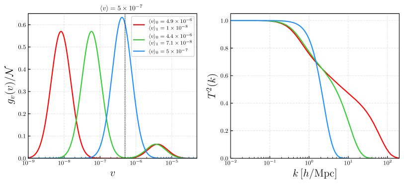
Figure 1: Three dark-matter velocity distributions $g_{v}(v)$ of the general form specified in Eq. (13) (left panel), all of which have the same average velocity $\langle v\rangle=5\times 10^{-7}$ and therefore the same nominal free-streaming scale $k_{\rm FSH}$, but lead to very different matter power spectra $P(k)$ (right panel). The blue curve in each panel corresponds to the case in which $\Omega_{1}=0$ and $g_{v}(v)$ consists of a single Gaussian peak with $\langle v\rangle_{0}=5\times 10^{-7}$. The red curve corresponds to the case of a bi-modal $g_{v}(v)$ distribution with $\Omega_{0}/\Omega_{\rm DM}=0.1$, $\langle v\rangle_{0}=4.9\times 10^{-6}$, and $\langle v\rangle_{0}=1.0\times 10^{-8}$. The green curve corresponds to the case of a bi-modal $g_{v}(v)$ distribution with $\Omega_{0}/\Omega_{\rm DM}=0.1$, $\langle v\rangle_{0}=4.4\times 10^{-6}$, and $\langle v\rangle_{0}=7.1\times 10^{-8}$. For all of these distributions, we have taken $\sigma_{0}=\sigma_{1}=0.63$. We observe from the right panel that the matter power spectra associated these latter $g_{v}(v)$ distributions differ significantly from the spectrum associated with the unimodal one.

While the results in Fig. 1 provide a qualitative picture of the extent to which the matter power spectra associated with complicated, multi-modal $g_{v}(v)$ distributions differ from those associated with narrow, unimodal such distributions, it is also illuminating to investigate these differences in a more systematic, quantitative manner. For example, it is interesting to assess the degree to which the matter power spectrum that follows from a given $g_{v}(v)$ distribution differs not merely from the $P(k)$ curve associated with one particular narrow, unimodal distribution, but from any such distribution.

In order to perform such an analysis for $g_{v}(v)$ distributions of the form given in Eq. (13), we begin by evaluating the transfer function $T^{2}(k)$ for the $g_{v}(v)$ distribution of interest using the CLASS code package. We then compare this distribution to a family of transfer functions obtained for a representative sample of narrow, unimodal $g_{v}(v)$ distributions. Since any two narrow, unimodal $g_{v}(v)$ distributions with the same $\langle v\rangle$ yield very similar matter power spectra, it is sufficient to include only $g_{v}(v)$ distributions associated with WDM models in this sample. To a very good approximation, the transfer function for a WDM model depends only on the mass $m_{\rm WDM}$ of the dark-matter particle and takes the form [20, 21, 22]

$$T_{\rm WDM}^{2}(k)~{}\approx~{}\left[1+(\alpha k)^{2\nu}\right]^{-10/\nu}\ ,$$ (14)

where $\nu=1.12$ and where

$$\alpha~{}=~{}\frac{0.049~{}{\rm Mpc}}{h}\left(\frac{m_{\rm WDM}}{\rm keV}\right)^{\!\!-1.11}\hskip-2.8903pt\left(\frac{\Omega_{\rm WDM}}{0.25}\right)^{\!\!0.11}\hskip-2.8903pt\left(\frac{h}{0.7}\right)^{\!\!1.22}~{}.$$ (15)

Thus, the family of transfer functions to which we shall compare $T^{2}(k)$ for our $g_{v}(v)$ distribution of interest consists of a sample of WDM transfer functions $T_{\rm WDM}^{2}(k)$ corresponding to different values of $m_{\rm WDM}$. In constructing this sample, we survey a broad range of $m_{\rm WDM}$ masses with a step size sufficiently small that further reducing that step size does not significantly impact our results.

For each value of $m_{\rm WDM}$ in this survey, we sample both the corresponding transfer function $T^{2}_{\rm WDM}(k)$ given by Eq. (14) and the transfer function $T^{2}(k)$ obtained for our double-peak $g_{v}(v)$ distribution at a series of wavenumbers $k_{j}$ separated by regular intervals in $(\log k)$-space within the range $0.1~{}h{\rm Mpc}^{-1}\leq k\leq 2000~{}h{\rm Mpc}^{-1}$. We assess the goodness of fit between the two curves using the chi-square statistic

$$\chi^{2}(m_{\rm WDM})~{}=~{}\sum_{j}\frac{[T^{2}(k_{j})-T^{2}_{\rm WDM}(k_{j})]^{2}}{\sigma_{T^{2}}^{2}(k_{j})}~{},~{}$$ (16)

where $\sigma_{T^{2}}(k_{j})$ is the uncertainty in the transfer function at $k_{j}$. For simplicity, since the choice of $\sigma_{T^{2}}(k_{j})$ values for this theoretical comparison is somewhat arbitrary, we take $\sigma_{T^{2}}(k_{j})$ to be equal to a common value $\sigma_{T^{2}}$ for all $k_{j}$. Under this assumption, $\sigma_{T^{2}}$ may be viewed simply as a normalization factor. We take the minimum value

$$\chi^{2}_{\rm min}~{}=~{}\underset{m_{\rm WDM}}{\min}\left\{\chi^{2}(m_{\rm WDM})\right\}$$ (17)

from among all of the $\chi^{2}(m_{\rm WDM})$ values obtained in this way to be our relative measure of the distinctiveness of $T^{2}(k)$.

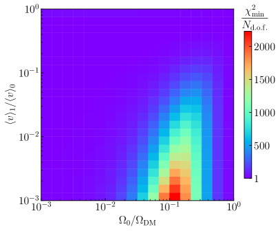
Figure 2: The minimum value $\chi^{2}_{\rm min}$ of the chi-square statistic obtained by fitting the linear matter power spectrum obtained for bi-modal dark-matter velocity distribution to the spectrum obtained for any WDM distribution, displayed in the $(\langle v\rangle_{1}/\langle v\rangle_{0},\Omega_{1}/\Omega_{0})$-plane. The results displayed here correspond to the parameter choices $\sigma_{0}=\sigma_{1}=0.63$ and $\langle v\rangle_{0}=10^{-6}$.

We can endow this goodness-of-fit statistic with a meaningful interpretation by choosing the normalization factor $\sigma_{T^{2}}$ in accord with the usual statistical expectation that $\chi^{2}_{\rm min}/N_{\rm d.o.f.}\sim 1$ when the fit between $T^{2}(k)$ and the optimal $T^{2}_{\rm WDM}(k)$ distribution in our sample is good, where $N_{\rm d.o.f.}$ is the number of degrees of freedom. Thus, we choose $\sigma_{T^{2}}$ such that $\chi^{2}_{\rm min}/N_{\rm d.o.f.}=1$ when $\Omega_{0}=1$ and $\sigma_{0}=0.63$ and the $g_{v}(v)$ distribution reduces to a unimodal distribution with a standard deviation equal to that of a WDM distribution. With this choice of normalization, $\chi^{2}_{\rm min}/N_{\rm d.o.f.}\sim\mathcal{O}(1)$ indicates that the matter power spectrum obtained from the corresponding double-peak $g_{v}(v)$ distribution does not differ significantly from that obtained in some WDM scenario, while $\chi^{2}_{\rm min}/N_{\rm d.o.f.}\gg 1$ indicates a significant difference.

In Fig. 2, we show the value of $\chi_{\rm min}^{2}/N_{\rm d.o.f.}$ within the $(\langle v\rangle_{1}/\langle v\rangle_{0},\Omega_{1}/\Omega_{\rm DM})$-plane for the $g_{v}(v)$ distribution in Eq. (13) with $\sigma_{0}=\sigma_{1}=0.63$ and $\langle v\rangle_{0}=10^{-6}$. We observe that there exists a sizable region of parameter space within which $\chi_{\rm min}^{2}/N_{\rm d.o.f.}\gg 1$ and the matter power spectrum obtained from the double-peak $g_{v}(v)$ distribution in Eq. (13) indeed differs significantly from that obtained from any WDM distribution. The largest values of $\chi_{\rm min}^{2}/N_{\rm d.o.f.}$ are obtained within regions of the plane wherein $\Omega_{0}$ is smaller than but not negligible in comparison with $\Omega_{1}$ and there is s significant separation between the mean velocities of the two peaks.

To summarize the results of this section, we have reviewed the physical principles behind the suppression of small-scale structure due to the free-streaming of dark-matter particles. We have demonstrated that while the variation of the horizon wavenumber $k_{\rm hor}(v)$ across the dark-matter velocity distribution has relatively little impact on $P(k)$ when $g_{v}(v)$ is unimodal and narrow, it can have an enormous impact on $P(k)$ for more general $g_{v}(v)$ distributions. Moreover, on the basis of the threshold relationship between $v$ and $k$ that exists by virtue of Eq. (10), we have been able to define an invertible map between these two variables — a map which can be exploited in order to extract information about $g_{v}(v)$ from $P(k)$ [5].

III From Matter Power Spectra to Halo-Mass Functions

Having summarized the relationship between $g_{v}(v)$ and $P(k)$, we now discuss the relationship between $P(k)$ and $dn/d\log M$. In relating these two quantities, we follow the analytic approach originally posited by Press and Schechter [6] and subsequently justified using the excursion-set formalism of Bond et al. [8].

At late times, regions of space with sufficiently large average overdensity collapse under their own gravity and form compact, virialized objects — i.e., matter halos. The probability that a randomly chosen spherical region of space with radius $R$ will collapse prior to a given cosmological time $t$ depends on the statistical properties of $\delta(\vec{\mathbf{x}},t)$. The crucial quantity in this regard is the spatial average $\sigma^{2}(t,R)$ of the variance of $\delta(\vec{\mathbf{x}},t)$ within the same region. This spatial average may be written as

$$\sigma^{2}(t,R)~{}\equiv~{}\int_{-\infty}^{\infty}d\log k\,\,W^{2}(k,R)\frac{k^{3}P(k,t)}{2\pi^{2}}~{},$$ (18)

where $W(k,R)$ is the Fourier transform in $k$-space of the position-space top-hat function $W(r,R)\equiv\Theta(1-r/R)$, where $\Theta(x)$ denotes the Heaviside function. This enforces the condition that only points at distances $r\leq R$ away from the center of the region are included in the average. However, this definition of $\sigma^{2}(t,R)$ may also be generalized to include other functional forms for $W(k,R)$. In this paper, we shall instead adopt a window function which is a top-hat function in $k$-space [23]:

$$W(k,R)~{}=~{}\Theta(1-kR)~{}.$$ (19)

One well-known advantage of the window function in Eq. (19) is that its flatness in $k$-space allows $\sigma^{2}(t,R)$ to be sensitive to the natural shape of the matter power spectrum itself, rather than that of $W(k,R)$ [24]. This window function also has other advantages. One of these is that only density perturbations with wavenumbers $k\leq R^{-1}$ have any effect on $\sigma^{2}(t,R)$. The primary drawback of this form of $W(k,R)$, however, is that the precise mathematical relationship between the value of $R$ associated with a halo and the corresponding halo mass $M$ is not well defined. Nevertheless, since symmetry considerations dictate that $M\propto R^{3}$, the relationship between $M$ and $R$ may be parametrized as

$$M~{}\equiv~{}\frac{4\pi}{3}\overline{\rho}(c_{W}R)^{3}~{},$$ (20)

where $\overline{\rho}$ is the present-day mass density of the universe and where the value of the coefficient $c_{W}$ may be obtained from the results of numerical simulations. Following Ref. [25], we take $c_{W}\approx 2.5$. The value of $\overline{\rho}=\Omega_{m}\rho_{\mathrm{crit}}$ can be determined from the total present-day matter abundance and critical density, which we take to be $\Omega_{m}\approx 0.315$ and $\rho_{\mathrm{crit}}\approx 2.775\times 10^{11}h^{2}~{}M_{\odot}{\rm Mpc}^{-3}$ [26], respectively. Given that a well-defined one-to-one relationship exists between $M$ and $R$, the spatially-averaged variance $\sigma^{2}(t,M)$ may also be viewed as a function of the halo mass $M$.

Within the Press-Schechter formalism, the present-day halo-mass function which follows from any particular $P(k)$ profile takes the form

$$\frac{dn}{d\log M}~{}=~{}\frac{\overline{\rho}}{2M}\eta(M)\frac{d\log\nu(M)}{d\log M}~{},$$ (21)

where $\nu(M)\equiv\delta_{c}^{2}/\sigma^{2}(t_{\mathrm{now}},M)$, with $\delta_{c}\approx 1.686$ denoting the critical overdensity, and where the function $\eta(M)$, which depends on $M$ only through the function $\nu(M)$, represents the probability density of obtaining an averaged fractional overdensity at a given location. For the window function in Eq. (19), regardless of the form of $\eta(M)$, the expression for $dn/d\log M$ in Eq. (21) simplifies to

$$\frac{dn}{d\log M}~{}=~{}\frac{\overline{\rho}}{12\pi^{2}M}\nu(M)\eta(M)\frac{P\big{(}1/R(M)\big{)}}{\delta_{c}^{2}R^{3}(M)}~{},~{}~{}~{}$$ (22)

where $R(M)$ is the particular value of $R$ which corresponds to a given halo mass $M$ through Eq. (20).

A variety of possible forms for the function $\eta(M)$ have been proposed, based either on purely theoretical grounds or based on the results of $N$-body or hydrodynamic simulations [6, 9, 10, 27, 28, 29, 30, 31, 32, 33]. In what follows, we adopt the form [9, 10]

$$\eta(M)~{}=~{}\sqrt{\frac{2\nu(M)}{\pi}}A\left[1+\nu^{-\alpha}(M)\right]e^{-\nu(M)/2}~{},$$ (23)

where $A\approx 0.3222$ and $\alpha=0.3$. This form for $\eta(M)$ is mathematically simple and accords reasonably well with the results of numerical simulations. We shall discuss the way in which alternative functional forms for $\eta(M)$ could affect the results of our analysis in Sect. VII.

In order to quantify the extent to which $dn/d\log M$ deviates from the corresponding result $(dn/d\log M)_{\rm CDM}$ that we would obtain for purely cold dark matter (CDM), we shall henceforth define the dimensionless structure-suppression function according to the relation

$$S(M)~{}\equiv~{}\sqrt{\frac{dn/d\log M}{(dn/d\log M)_{\rm CDM}}}~{}.$$ (24)

This function may be viewed as playing an analogous role with respect to the halo-mass function that the transfer function $T(k)$ plays with respect to the linear matter power spectrum. Moreover, for the Press-Schechter halo-mass function in Eq. (22), we find that $S^{2}(M)$ and $T^{2}(k)$ are related in any given dark-matter model by

$$S^{2}(M)~{}=~{}\frac{\nu(M)\eta(M)}{\nu_{\rm CDM}(M)\eta_{\rm CDM}(M)}T^{2}(1/R(M))~{},$$ (25)

where $\nu(M)$ and $\eta(M)$ are obtained from the corresponding matter power spectrum $P(k)$ for the dark-matter model in question.

By examining the mathematical relationship between $g_{v}(v)$ and $S^{2}(M)$, we may hope to develop some intuition about the manner in which the detailed shape of the dark-matter velocity distribution affects the statistical properties of dark-matter halos and subhalos. As a first step toward developing that intuition, we begin by examining the relationship between $k$ and the halo mass $M$. The underlying reason we were able to construct a map between $v$ and $k$ in Sect. II is that $k_{\rm hor}(v)$ represents the threshold value of $k$ below which dark-matter particles with momentum $v$ cannot suppress structure by free-streaming. Fortunately, a similar relationship exists between $k$ and $M$ by virtue of the window function $W(k,R)$. Indeed, we see from the relationship between $R$ and $M$ in Eq. (20) that $W(k,R)$ establishes a threshold value of $M$ for any given wavenumber $k$ above which density perturbations with that value of $k$ have no effect on $\sigma^{2}(t_{\mathrm{now}},M)$ and therefore no effect on the halo-mass function. In particular, we see from Eqs. (19) and (20) that this threshold value of $M$ is specified by the function

$$M_{\rm hal}(k)~{}\equiv~{}\frac{4\pi}{3}\overline{\rho}\left(\frac{c_{W}}{k}\right)^{3}~{}.$$ (26)

Just as we regarded Eq. (10) as defining a functional map between $v$ and $k$, we shall likewise regard Eq. (26) as defining a functional map between $k$ and $M$. As with our map between $v$ and $k$, this map between $k$ and $M$ is likewise one-to-one and invertible.

We note that the threshold relationship between $k$ and $M$ which have used in in constructing the functional map in Eq. (26) is only precisely defined for a window function with a sharp cutoff in $k$ which decreases with increasing $M$. Indeed, this is one of the reasons why we have adopted the form for $W(k,R)$ in Eq. (19) in this analysis. However, this does not mean that a heuristic functional map between $k$ and $M$ cannot be defined for other forms of $W(k,R)$ as well. Indeed, by construction any sensible functional form for $W(k,R)$ must like serve to suppress the contribution to $\sigma^{2}(t,R)$ from small-scale fluctuations with wavenumbers $k\gg R^{-1}$. Thus, even in cases in which $W(k,R)$ does not have a sharp cutoff in $k$, a qualitative threshold relationship exists between $k$ and $M$ which can be used to formulated an invertible functional map between these variables. In such cases, one could account for the ambiguity in the cutoff by incorporating an additional overall proportionality factor into Eq. (26) analogous to the parameter $\xi$ in Eq. (10), the optimal value of which would likewise be determined empirically. We emphasize that this proportionality factor is not necessarily equivalent to the quantity $c_{W}^{3}$ that appears in Eq. (26) as a consequence of ambiguities in the relationship between $M$ and $R$, but that $c_{W}^{3}$ could of course be incorporated into this factor.

Combining the two functional maps in Eqs. (10) and (26) and taking the $a_{\rm prod}\rightarrow 0$ limit appropriate for particles which are relativistic at production, we can likewise define a direct functional map between $v$ and $M$, which takes the form

$$M_{\rm hal}(v)~{}\equiv~{}\frac{4\pi\bar{\rho}c_{W}^{3}}{3\xi^{3}}\left[\int_{0}^{1}\frac{da}{Ha^{2}}\frac{\gamma v}{\sqrt{\gamma^{2}v^{2}+a^{2}}}\right]^{3}~{}.~{}$$ (27)

As with the individual maps in Eqs. (10) and (26), this map is one-to-one and invertible.

The physical motivation for defining $M_{\rm hal}(v)$, which we plot in Fig. 3, is that it conveys information about what parts of $g_{v}(v)$ are capable of affecting the halo-mass function at a given mass scale. Dark-matter particles with velocities below a given value $v$ can only suppress structure at wavenumbers $k>k_{\rm hor}^{-1}(v)$ and can therefore only affect the number density of halos with masses $M<M_{\rm hal}(k_{\rm hor}^{-1}(v))$. Thus, the value of $M$ associated with a given value of $v$ through Eq. (27) represents the maximum halo mass for which dark-matter particles with that velocity can affect $S^{2}(M)$.

Figure 3: The halo-mass variable $M_{\rm hal}(v)$, as defined in Eq. (27), plotted as a function of $v$. The purple shaded region corresponds to the range of $M$ shown in Fig. 10.

Some comments about this functional map between $v$ and $M$ are in order. First, we may use this map in order to perform a change of variables and define a velocity distribution in $M$-space which corresponds to the distribution $g_{v}(v)$ in $v$-space. In particular, by changing variables from $v$ to $M$ in Eq. (2), we find that

$$N(t)~{}=~{}\frac{g_{\rm int}}{2\pi^{2}}\int d\log Mg_{M}(M)~{},~{}$$ (28)

where

$$g_{M}(M,t)~{}\equiv~{}g_{v}\big{(}M^{-1}_{\rm hal}(M),t\big{)}\left|\frac{d\log v}{d\log M_{\rm hal}(v)}\right|~{},$$ (29)

where the factor $\left|d\log v/d\log M(v)\right|$ is simply the Jacobian for this change of variables. This $M$-space velocity distribution in Eq. (29) has a straightforward physical meaning. In particular, up to an overall factor of $g_{\rm int}/2\pi$, this distribution is simply the differential number density of dark-matter particles per unit $\log M$ with velocities just barely sufficient to free-stream out of regions of space within which the dark matter would otherwise collapse into halos of mass $M$.

One advantage of defining $g_{M}(M)$ is that it can be used to facilitate a direct graphical comparison between the features of the the dark-matter velocity distribution and the features of $S^{2}(M)$. Since $g_{M}(M)$ is also a function of $M$, it can be plotted on the same axes as the structure-suppression function. As we shall see, juxtaposing $g_{M}(M)$ and $S^{2}(M)$ in this way can provide valuable insights into the relationship between these two functions.

Another advantage of defining $g_{M}(M)$ in this way is that it allows us to characterize the fraction of dark-matter particles which are “hot” relative to the mass scale $M$ — i.e., capable of free-streaming out of regions which would collapse into halos of mass $M$ — in a straightforward manner. The threshold velocity above which dark-matter particles can free-stream out of such regions is $v=M^{-1}_{\rm hal}(M)$. The portion of $g_{v}(v^{\prime})$ with velocities $v^{\prime}>v$ above this threshold corresponds to the portion of $g_{M}(M^{\prime})$ with $M^{\prime}>M$. Thus, up to an overall proportionality constant, the number density of dark-matter particles with velocities sufficient to free-stream out of halos of mass $M$ can be obtained by integrating $g_{M}(M^{\prime})$ over $M^{\prime}$ above this threshold. Motivated by this consideration, we define the hot-fraction function

$$F(M)~{}\equiv~{}\frac{\int_{\log M}^{\infty}d\log M^{\prime}\,g_{M}(M^{\prime})}{\int_{-\infty}^{\infty}d\log M^{\prime}\,g_{M}(M^{\prime})}~{},~{}$$ (30)

which represents the fraction of the total dark-matter abundance associated with these particles.

IV Halo-Mass Functions for Non-Trivial Dark-Matter Velocity Distributions

We shall now examine how the detailed shape of $g_{v}(v)$ affects the shape of the halo-mass function within the context of the analytic formalism outlined in Sect. III. In doing so, we shall begin by focusing on a comparatively simple form for $g_{v}(v)$ which can be modified in a controlled way and assessing the effect of these modifications on $S^{2}(M)$. In particular, we shall consider the limiting case of Eq. (13) in which and $\sigma_{1}$ is narrow and $\langle v\rangle_{1}$ is sufficiently small that the dark-matter particles associated with the lower-velocity peak behave like CDM. In this limit, the $g_{v}(v)$ distribution reduces to a single Gaussian peak accompanied by a purely cold component which makes up the remainder of $\Omega_{\rm DM}$. This single peak is characterized by only three parameters: its average velocity $\langle v\rangle_{0}$, width $\sigma_{0}$, and abundance $\Omega_{0}$.

In Fig. 5, we illustrate the effect of varying $\Omega_{0}$ while holding its width $\sigma_{0}$ and average velocity $\langle v\rangle_{0}$ fixed. In the left panel, we show the $g_{v}(v)$ distributions obtained for several such distributions with different $\Omega_{0}$ values as functions of $v$. In the right panel, we show both the corresponding distributions $g_{M}(M)$ that we obtain from our functional map between $v$ and $M$ as functions of $M$ and the corresponding structure-suppression functions $S^{2}(M)$.

Moving from right to left across the right panel of Fig. 5, we observe that the $S^{2}(M)$ remains effectively unsuppressed in the region to the right of the peak in $g_{M}(M)$. More importantly, we also observe that that the logarithmic slope $d\log S^{2}(M)/d\log M$ of the structure-suppression function in the region immediately to the left of the peak appears to be correlated with the abundance $\Omega_{0}$.

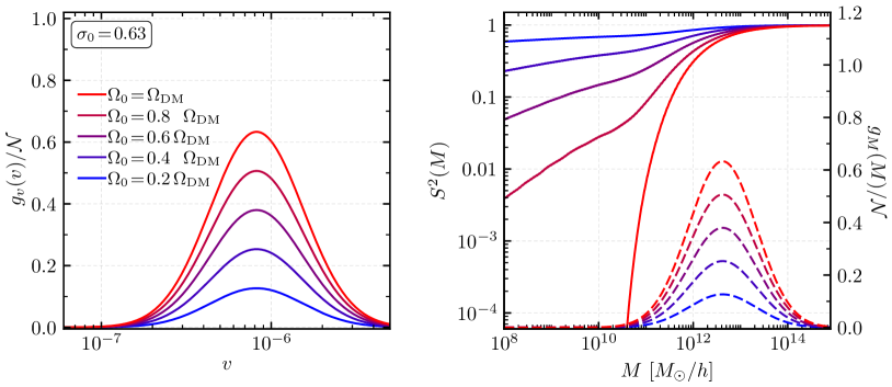
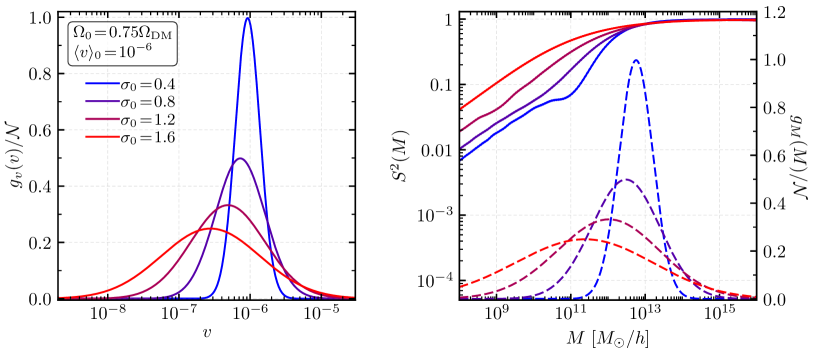
Figure 4: Several dark-matter velocity distributions, each consisting of a single Gaussian peak with a different fractional abundance $\Omega_{0}/\Omega_{\rm DM}$ and a purely cold component which contributes the remainder of $\Omega_{\rm DM}$, along with the corresponding structure-suppression functions $S^{2}(M)$. The left panels shows the $g_{v}(v)$ distributions as functions of $v$; the right panel shows both the corresponding distributions $g_{M}(M)$ that we obtain from our functional map between $v$ and $M$ as functions of $M$ and the $S^{2}(M)$ curves that we obtain for these distributions. For each of the distributions shown, we have taken $\sigma_{0}=0.63$ and $\langle v\rangle_{0}=10^{-6}$. We observe that the logarithmic slope $d\log S^{2}(M)/d\log M$ of the structure-suppression function at small $M$ is correlated with the total abundance of dark-matter particles in the $g_{M}(M^{\prime})$ distribution with $M^{\prime}>M$.

Figure 5: Similar to Fig. 5, but for a set of dark-matter velocity distributions in which the width $\sigma_{0}$ of the Gaussian peak is varied while the total abundance $\Omega_{0}=\Omega_{\rm DM}$ and average velocity $\langle v\rangle_{0}=10^{-6}$ are held fixed. We observe that the value of $S^{2}(M)$ in the region to the left of the peak in $g_{M}(M)$ is sensitive to the width of the peak, the value of $d\log S^{2}(M)/d\log M$ in this same region is not.

In Fig. 5, we illustrate the effect of varying the width $\sigma_{0}$ of the Gaussian peak while holding its abundance $\Omega_{0}=\Omega_{\rm DM}$ and average velocity $\langle v\rangle_{0}$ fixed. We emphasize that since each Gaussian peak in Eq. (13) is centered at $\log\langle v\rangle_{i}-\sigma_{i}^{2}/2$ in ($\log v$)-space, the location of the peak in $g_{v}(v)$ shown in the left panel of the figure shifts to the left as the corresponding $\sigma_{0}$ increases. A corresponding shift is of course also evident in the $g_{M}(M)$ distributions shown in the right panel.

We observe that that increasing $\sigma_{0}$ induces to a more gradual suppression of $S^{2}(M)$ as we move from right to left across the right panel of Fig. 5, ultimately resulting in less net suppression in $S^{2}(M)$ at small values of $M$. However, we also observe that while the value of $S^{2}(M)$ in the region to the left of the peak in $g_{M}(M)$ is sensitive to the width of the peak, the logarithmic slope $d\log S^{2}(M)/d\log M$ in that same region is not.

Taken together, the results shown in Figs. 5 and 5 suggest that the value of $d\log S^{2}(M)/d\log M$ at any given value of $M$ is correlated with the total abundance contribution associated with the portion of $g_{M}(M^{\prime})$ with $M^{\prime}>M$. This total abundance contribution is simply $\Omega_{\rm DM}F(M)$, where $F(M)$ is the hot-fraction function in Eq. (30). Indeed, an equivalent statement of this conjecture, which follows from the invertible map in Eq. (27), is that the value of $d\log S^{2}(M)/d\log M$ is correlated with the total abundance contributed by dark-matter particles within $g_{v}(v^{\prime})$ with velocities $v^{\prime}>v$, where $v=M^{-1}_{\rm hal}(M)$ is the threshold velocity associated with $M$ by the inverse of this map.

In order to test this conjecture further, we now consider more complicated $g_{v}(v)$ distributions in which both Gaussian peaks in Eq. (13) occur at velocities large enough to have a significant impact on structure. In Fig. 7, we illustrate the effect of varying $\langle v\rangle_{1}$ of the lower-velocity peak while holding $\langle v\rangle_{0}=10^{-6}$, the widths $\sigma_{0}=\sigma_{1}=0.63$, and the abundances $\Omega_{0}=\Omega_{1}$ fixed. The blue curve in the left panel represents the case in which $\langle v\rangle_{1}=\langle v\rangle_{0}$ and the two peaks in $g_{v}(v)$ coincide, effectively yielding a single Gaussian. By contrast, the green, yellow, and red curves represent $g_{v}(v)$ distributions with successively greater distances between $\langle v\rangle_{1}$ and $\langle v\rangle_{0}$. The corresponding $S^{2}(M)$ curves and $g_{M}(M)$ distributions are shown in the right panel of the figure.

We observe that the $S^{2}(M)$ curves obtained for the the $g_{v}(v)$ distributions in which there is a significant separation between the peaks qualitatively differ from the curves obtained for narrow, unimodal $g_{v}(v)$ distributions. Moreover, these curves provide additional insight into the relationship between $S^{2}(M)$ and $g_{M}(M)$. For example, we observe that $d\log S^{2}(M)/d\log M$ at a location $M$ immediately to the left of each peak in $g_{M}(M)$ is correlated with the value of $F(M)$ at such locations. Indeed, as we scan from larger to smaller values of $M$ across either of the peaks in a given $g_{M}(M)$ distribution, we see that $d\log S^{2}(M)/d\log M$ becomes increasingly steep as the cumulative abundance associated with dark-matter particles whose speeds $v$ map to halo masses above $M$ increases. By contrast, as we scan from larger to smaller values of $M$ across the region between each pair of peaks, where $g_{M}(M)$ is negligible, we see that $d\log S^{2}(M)/d\log M$ either remains constant or increases. Indeed, this is the case regardless of how much separation there is between the peaks.

The behavior of the curves in the right panel of Fig. 7 also illustrates the “locality” inherent in the relationship between $g_{M}(M)$ and $S^{2}(M)$. If two $g_{v}(v^{\prime})$ distributions are identical above some velocity $v$, but differ for $v^{\prime}<v$, the corresponding $S^{2}(M^{\prime})$ distributions differ only for masses $M^{\prime}<M(v)$. As a result, any two structure-suppression functions shown in Fig. 7 coincide almost perfectly at large $M$, and continue to track each other as $M$ decreases, all the way down to the point which the corresponding $g_{M}(M)$ distributions begin to diverge. We emphasize that this is true regardless of whether $d^{2}\log S^{2}(M)/(d\log M)^{2}$ is negative throughout the range of $M$ above which the two $g_{M}(M)$ distributions coincide. Indeed, it still holds even if $d^{2}\log S^{2}(M)/(d\log M)^{2}\geq 0$ across some or all of this range.

Figure 6: Similar to Fig. 5, but for a set of double-peak dark-matter velocity distributions in which the average velocity $\langle v\rangle_{1}$ of the lower-velocity peak is varied, while $\langle v\rangle_{0}=10^{-6}$, the widths $\sigma_{0}=\sigma_{1}=0.63$, and the abundances $\Omega_{1}=\Omega_{2}=\Omega_{\rm DM}/2$ are all held fixed. We observe that as we scan from right to left across the right panel of the figure, any two $d\log S^{2}(M)/d\log M$ curves coincide up until the point at which the corresponding $g_{M}(M)$ distributions begin to differ.

Figure 7: Similar to Fig. 5, but for a set of double-peak dark-matter velocity distributions of in which the abundances $\Omega_{0}$ and $\Omega_{1}$ associated with the two peaks are varied, while $\langle v\rangle_{0}=2\times 10^{-6}$, $\langle v\rangle_{1}=10^{-8}$, the widths $\sigma_{0}=\sigma_{1}=0.63$, and the sum $\Omega_{0}+\Omega_{1}=\Omega_{\rm DM}$ of these abundances are all held fixed. We observe that $d\log S^{2}(M)/d\log M$ at a location $M$ immediately to the left of any individual peak in $g_{M}(M)$ is correlated with the value of $F(M)$ at that same location.

Finally, in Fig. 7, we illustrate the effect on $S^{2}(M)$ of varying the relative abundances associated with the two peaks while holding $\langle v\rangle_{0}=2\times 10^{6}$, $\langle v\rangle_{1}=10^{8}$, and the widths $\sigma_{0}=\sigma_{1}=0.63$ fixed. As in Fig. 7, we see that $d\log S^{2}(M)/d\log M$ decreases as we scan from larger to smaller values of $M$ across any particular peak in $g_{M}(M)$, but that it remains constant or increases as we scan across regions in which $g_{M}(M)$ is negligible. However, we also see that the corresponding change in $d\log S^{2}(M)/d\log M$ is indeed correlated with $F(M)$.

Indeed, taken together, the results shown in Figs. 5—7 suggest that there is a direct relationship between $d\log S^{2}(M)/d\log M$ and $F(M)$. In particular, as we shall demonstrate explicitly in Sect. VI, we find that within any interval in $M$-space at which $g_{M}(M)$ is non-negligible, this relationship is well described by a simple empirical relation of the form

$$\frac{d\log S^{2}(M)}{d\log M}~{}\approx~{}\frac{7}{10}\,F^{2}(M)~{}.$$ (31)

Since $F(M)$ is by definition a monotonically decreasing function of $M$, this relation implies that $d^{2}\log\,S^{2}(M)/(d\log M)^{2}\leq 0$ within any such interval. We stress that this empirical relation is quite robust and holds regardless of how complicated the dark-matter velocity distribution might be.

We also note that in cases in which the features in the dark-matter velocity distribution are well clustered in $M$-space — i.e., in which there are no extended intervals of $M$-space within which $g_{M}(M)\approx 0$ between these features — we may obtain an approximate expression for $S^{2}(M)$ itself by integrating Eq. (31) directly:

$$\log S^{2}(M)~{}\approx~{}\frac{7}{10}\int_{\log M}^{\infty}d\log M^{\prime}\,F^{2}(M^{\prime})$$

$$~{}~{}~{}=~{}\frac{7}{10}\int_{\log M}^{\infty}d\log M^{\prime}\left[\frac{1}{\mathcal{N}}\int_{\log M^{\prime}}^{\infty}d\log M^{\prime\prime}g_{M}(M^{\prime\prime})\right]^{2}~{}.$$

(32)

Moreover, as a consequence to the locality inherent in the relationship between $g_{M}(M)$ and $S^{2}(M)$, this procedure may also be applied to more general dark-matter velocity distributions in order to derive an an approximation for $S^{2}(M)$ at values of $M$ above all such extended intervals. Such an approximation is potentially useful, as is would enable one to circumvent the rather complex procedure outlined in Sect. III through which the calculation of $S^{2}(M)$ is normally performed. Of course, the usefulness of this approach will ultimately depend on the precision with which one might seek to evaluate $S^{2}(M)$.

The precise mathematical form of Eq. (31) and the value of the numerical constant of course depend on the particular choice for the function $\eta(M)$ specified in Eq. (23). Nevertheless, we emphasize that a similar mathematical relationship between $S^{2}(M)$ and $g_{M}(M)$ will exist for any alternative functional form of $\eta(M)$ which likewise respects the physical thresholds that served as the basis for our functional map between $v$ and $M$ in Eq. (27). Indeed, this relationship is a consequence of locality — i.e., the fact that $d\log S^{2}(M)/d\log M$ is sensitive only to the portion of $g_{M}(M^{\prime})$ for which $M^{\prime}>M$. As we have seen, this locality ultimately stems from the assumption inherent in Eq. (21) that $\eta(M)$ depends on $M$ only through quantities which respect these physical thresholds.

That said, given that a full $N$-body analysis of the class of highly non-trivial $g_{v}(v)$ distributions that we are considering in this paper has never been performed, one might wonder whether this property of $\eta(M)$ still holds for these $g_{v}(v)$ distributions. While a conclusive answer to this question cannot be obtained without extensive numerical simulation, there are nevertheless indications that $\eta(M)$ indeed respects the same thresholds, even for more complicated forms of $g_{v}(v)$. For example, an $N$-body analysis of the kinds of halo-mass functions which arise in so-called mixed-dark-matter scenarios — i.e., scenarios in which the dark-matter velocity distribution includes both a WDM and a CDM contribution — was performed in Ref. [34]. Despite the more complicated form of $g_{v}(v)$ which characterizes these scenarios, the resulting $dn/d\log M$ were nevertheless found to be well modeled by an analytic function of the general form Eq. (21) with a universal $\eta(M)$ function which respects the relevant physical thresholds.

V Connecting to Observables

While the effect that the detailed shape of $g_{v}(v)$ on $S^{2}(M)$ has on the $S^{2}(M)$ is interesting in its own right, it is also interesting to extend this analysis a step further and consider how this detailed shape affects astrophysical observables which serve as probes of structure in the non-linear regime. We focus here on two such observables: satellite counts within the halos of large galaxies and cluster-number counts. As we shall see, the detailed shape of the dark-matter velocity distribution can have a non-trivial impact on both of these observables.

V.1 Satellite Counts

One observable which which provides information about the spatial distribution of matter within the universe is the number of satellite galaxies $N_{\rm SH}$ with masses $M$ above some observability threshold $M_{\rm min}$ which reside within a typical host halo of mass $M_{0}$. Of particular interest is the number of satellite galaxies within the halo of the Milky Way.

A theoretical prediction for $N_{\rm SH}$ can be derived analytically for a given $g_{v}(v)$ distribution and a given value of $M_{0}$. This prediction is derived not from the halo-mass function, but rather from the conditional mass function $dN(M,z|M_{0},z_{0})/dM$. This latter quantity represents the differential number of halos per unit mass $M$ present in the universe at redshift $z$ which, on average, will have been incorporated into a single host halo of mass $M_{0}$ by the time the universe reaches the redshift $z_{0}<z$. An approximate analytic expression for $dN(M,z|M_{0},z_{0})/dM$ can be derived from the same excursion-set formalism [8] from which Eq. (21) can be obtained. In particular, it can be shown that [35]

$$\frac{dN(M,z|M_{0},z_{0})}{dM}=-\frac{M_{0}}{M}\sigma^{2}(M)\zeta(M,z|M_{0},z_{0})\frac{d\sigma^{2}(M)}{dM}\,,~{}~{}$$ (33)

where $\sigma^{2}(M)\equiv\sigma^{2}(t_{\mathrm{now}},M)$ and where $\zeta(M,z|M_{0},z_{0})$ represents the probability that a particle present in a halo of mass $M$ at redshift $z$ would have been incorporated into a halo of mass $M_{0}$ by the time the universe reaches redshift $z_{0}$. Under the simplifying assumption of spherical collapse, this conditional probability takes the analytic form

$$\zeta(M,t|M_{0},t_{0}) = \frac{\delta(z)-\delta(z_{0})}{(2\pi)^{1/2}[\sigma^{2}(M)-\sigma^{2}(M_{0})]^{3/2}}$$ (34)

$$\times~{}\exp\left(-\frac{[\delta(z)-\delta(z_{0})]^{2}}{2[\sigma^{2}(M)-\sigma^{2}(M_{0})]}\right)\,,~{}~{}~{}~{}~{}~{}$$

where $\delta(z)\equiv\delta_{c}/D(z)$ is defined in terms of the universal growth factor $D(z)$ for perturbations at redshift $z$.

In order to estimate the number of subhalos with masses above a given threshold, we follow the procedure outlined in Refs. [36, 25]. We integrate the conditional mass function over $z$ in order to obtain the differential number $dN_{\rm SH}/dM$ of subhalos per unit $M$:

$$\frac{dN_{\rm SH}}{dM}~{}=~{}\frac{1}{\mathcal{N}_{\rm SH}}\int_{0}^{\infty}\frac{dN(M,t|M_{0},t_{0})}{dM}\frac{d\delta(z)}{dz}dz~{},~{}$$ (35)

where $\mathcal{N}_{\rm SH}$ is a normalization factor which accounts for the fact that this integration overcounts the number of halos by including the same progenitor at multiple redshifts. Thus, the total expected number of subhalos with masses above a given mass threshold $M_{\rm min}$ within a host halo of mass $M_{0}$ is

$$N_{\rm SH}~{}=~{}\int_{M_{\rm min}}^{M_{0}}\frac{dN_{\rm SH}}{dM}dM~{}.$$ (36)

In order to assess the degree to which $N_{\rm SH}$ depends on the detailed shape of the dark-matter velocity distribution, we evaluate the predicted number of Milky-Way satellites for a variety of $g_{v}(v)$ distributions of the form given in Eq. (13) using Eq. (36). For the window function in Eq. (19), the expression in Eq. (35) reduces to

$$\frac{dN_{\rm SH}}{dM} ~{}=~{} \frac{1}{6\pi^{2}\mathcal{N}_{\rm SH}}\left(\frac{M_{0}}{M^{2}}\right)$$ (37)

$$\times~{}\frac{P(1/R(M))}{R^{3}(M)\sqrt{2\pi[\sigma^{2}(M)-\sigma^{2}(M_{0})]}}~{}.~{}~{}~{}$$

We choose this normalization factor $\mathcal{N}_{\rm SH}$ such that the value of $N_{\rm SH}$ obtained from Eq. (36) for a Milky-Way-sized galaxy in a purely CDM scenario accords with the value obtained from $N$-body simulations. In particular, we base our value of $\mathcal{N}_{\rm SH}$ on the results obtained by Aquarius project [37], which obtained a value $N_{\rm SH}=157$ for the number of subhhalos of mass $M>10^{8}\,h^{-1}M_{\odot}$ in a Milky-Way-like galaxy of mass $M_{0}=1.77\times 10^{12}\,h^{-1}M_{\odot}$. Accordingly, we adopt $M_{\rm min}=10^{8}\,h^{-1}M_{\odot}$ as our mass threshold. For this value of $M_{\rm min}$, we find numerically that $\mathcal{N}\approx 46.9$, which is roughly similar to the result $\mathcal{N}_{\rm SH}=44.5$ obtained in Ref. [25].

In order to present the results of this analysis in an illustrative way, we shall also define the quantity $N_{\rm SH}^{\rm WDM}(k_{\rm FSH})$ for a given $g_{v}(v)$ distribution to represent the value of $N_{\rm SH}$ that one would obtain for a WDM velocity distribution with the same average velocity $\langle v\rangle$ as $g(v)$ — and hence also the same nominal free-streaming scale $k_{\rm FSH}$. Since the dark-matter velocity distribution for a WDM model is completely specified by the single parameter $m_{\rm WDM}$, $N_{\rm SH}^{\rm WDM}(k_{\rm FSH})$ is uniquely defined. The ratio

$${\large\textcjheb{+s}}~{}\equiv~{}\frac{N_{\rm SH}}{N_{\rm SH}^{\rm WDM}(k_{\rm FSH})}$$ (38)

of the actual value of $N_{\rm SH}$ obtained for this $g_{v}(v)$ to the value of $N_{\rm SH}^{\rm WDM}(k_{\rm FSH})$ quantifies the degree to which $N_{\rm SH}$ departs from the WDM result due to the detailed shape of $g_{v}(v)$.

In the left panel of Fig. 8, we show contours within the $(\Omega_{0}/\Omega_{\rm DM},\langle v\rangle_{0}/\langle v\rangle_{1})$-plane of the expected number of satellite galaxies with masses $M>10^{8}\,h^{-1}M_{\odot}$ contained within a Milky-Way-sized galaxy of mass $M_{0}=1.77\times 10^{12}\,h^{-1}M_{\odot}$. The results shown here correspond to the parameter choices $\langle v\rangle_{0}=10^{-6}$ and $\sigma_{0}=\sigma_{1}=0.63$. In the right panel, we show contours of the ratio +s  within the $(\Omega_{0}/\Omega_{\rm DM}\langle v\rangle_{0}/\langle v\rangle_{1})$-plane for the same choice of parameters. In each panel, we have also included contours (dashed black lines) of the nominal free-streaming scale $k_{\rm FSH}$.

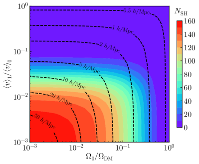
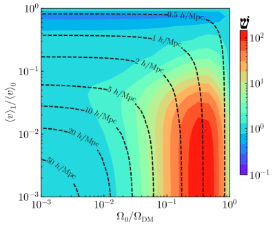
Figure 8: Left panel: The expected number $N_{\rm SH}$ of satellites with masses $M>10^{8}\,h^{-1}M_{\odot}$ within the halo of a Milky-Way-sized galaxy for a dark-matter scenario with a velocity distribution given by Eq. (13), displayed within the $(\Omega_{0}/\Omega_{\rm DM},\langle v\rangle_{0}/\langle v\rangle_{1})$-plane. The results shown in the figure correspond to the parameter choices $\langle v\rangle_{0}=10^{-6}$ and $\sigma_{0}=\sigma_{1}=0.63$. Right panel: The ratio +s of $N_{\rm SH}$ to the number of satellites obtained for the WDM model with the same nominal free-streaming scale $k_{\rm FSH}$, likewise displayed within the $(\Omega_{0}/\Omega_{\rm DM},\langle v\rangle_{0}/\langle v\rangle_{1})$-plane. Contours of $k_{\rm FSH}$ (dashed black lines) are also provided in each panel for reference.

In interpreting these results displayed in Fig. 8, we begin be noting that we may establish a rough bound on $g_{v}(v)$ by requiring that $N_{\rm SH}$ accord with the number $N_{\rm SH}^{\rm(obs)}$ actually observed in the halo of the Milky Way. The known Milky-Way satellites with masses above our $M_{\rm min}$ threshold include 11 classical satellites and 15 ultra-faint satellites discovered by the Sloan Digital Sky Survey (SDSS), as well as a number of additional satellites identified by the Dark Energy Survey (DES) [38, 39, 40, 41]. However, the current catalogue of $\sim 50$ such satellites is presumably highly incomplete, given that SDSS and DES do not together cover the entire sky and are subject to flux thresholds. We therefore estimate $N_{\rm SH}^{\rm(obs)}$ by multiplying the number of SDSS satellites by 3.5 in order to account for the limited sky coverage of the SDSS [42, 25, 43] and adding to this the number of classical satellites. This accounting yields $N_{\rm SH}^{\rm(obs)}=62$ for the total number of Milky-Way subhalos with masses $M>M_{\rm min}$.

The results shown in the right panel of Fig. 8 reflect the extent to which the detailed shape of $g_{v}(v)$ affects the value of $N_{\rm SH}$. The ratio +s  differs significantly from unity within the region wherein $\Omega_{0}/\Omega_{\rm DM}$ is large and $\langle v\rangle_{1}/\langle v\rangle_{0}\leq 0.1$ — in some places by as much as two orders of magnitude. These results make it clear that the detailed shape of $g_{v}(v)$ can have a significant impact on the substructure of galactic halos.

In addition to the rough lower bound on $N_{\rm SH}$, other considerations related to structure formation likewise constrain on the form of $g_{v}(v)$. For example, Lyman-$\alpha$-forest data impose stringent constraints on the shape of the matter power spectrum at wavenumbers $1\,h/{\rm Mpc}\lesssim k\lesssim 50\,h/{\rm Mpc}$. These constraints likewise depend of the detailed shape of $g_{v}(v)$. Constraints on $g_{v}(v)$ distributions of the form in Eq. (13) were derived in Ref. [44]. For the values of $\langle v\rangle_{0}$, $\sigma_{0}$, and $\sigma_{1}$ we have adopted in Fig. 8, an analysis employing the area criterion $\delta A$ [45] excludes the region of the $(\Omega_{0}/\Omega_{\rm DM},\langle v\rangle_{0}/\langle v\rangle_{1})$-plane wherein $\Omega_{0}/\Omega_{\rm DM}\gtrsim 0.1$ and $\langle v\rangle_{1}/\langle v\rangle_{0}\gtrsim 0.25$. While this excludes the region wherein +s is significantly below unity, the allowed region of parameter space includes sizable regions wherein ${\large\textcjheb{+s}}\sim\mathcal{O}(10-100)$.

V.2 Cluster-Number Counts

Another observable which provides information about the spatial distribution of matter within the universe is the number of galaxy clusters $N_{\rm C}$ observed within a given region of the sky. However, unlike satellite counts, cluster-number counts of this sort are directly related to the halo-mass function and therefore serve as a probe of $S^{2}(M)$ — and thus to the results derived in Sect. IV.

Observationally speaking, the cluster-number count obtained from a given survey is simply the total number of galaxy clusters observed within a particular region of the sky out to some maximum redshift $z_{\rm max}$ with masses which lie above some threshold $M_{\rm min}(z)$ which may be redshift-dependent. Thus, a theoretical prediction for $N_{\rm C}$ within a given dark-matter scenario may be obtained by evaluating [46]

$$N_{\rm C}~{}=~{}\int_{0}^{z_{\rm max}}z\frac{dV}{dz}\int_{\log M_{\rm min}(z)}^{\infty}d\log M\frac{dn}{d\log M}~{},$$ (39)

where $dV/dz$ is the comoving volume element per unit $z$. This comoving volume element may be written in the form

$$\frac{dV}{dz}~{}=~{}4\pi\Delta\Omega\frac{c\chi^{2}(z)}{H(z)}~{},~{}$$ (40)

where $\Delta\Omega$ is solid angle on the sky under observation, where $c$ is the speed of light, where $\chi(z)$ is the comoving distance, and where $H(z)$ is the Hubble parameter.

In assessing the cluster-number count which follows from any particular $g_{v}(v)$ distribution, we adopt a set of parameters which allow us to compare our predictions with results predicted for the Euclid survey [47]. In particular, we take $\Delta\Omega\approx 4.57$ sr and $z_{\rm max}=2$ and we we adopt the redshift-dependent detection mass threshold presented in Ref. [47], in which $M_{\rm min}(z)$ varies between $\sim 10^{13.8}$ and $10^{14.1}~{}M_{\odot}$.

In order to examine the effect of the primordial dark-matter velocity distribution on $N_{\rm C}$, we shall once again consider $g_{v}(v)$ distributions of the form given in Eq. (13). Moreover, since our aim is to highlight the effect of varying the detailed shape of $g_{v}(v)$, rather than the effect of varying the nominal free-streaming scale $k_{\rm FSH}$, we shall proceed by examining how $N_{\rm C}$ varies along surfaces of fixed $k_{\rm FSH}$ within our parameter space. In order that we may compare our results for $N_{\rm C}$ to those we have obtained for $N_{\rm SH}$ in a straightforward manner, we shall once again take $\langle v\rangle_{0}=10^{-6}$ and $\sigma_{0}=\sigma_{1}=0.63$ and focus on the effect of varying $\Omega_{0}/\Omega_{\rm DM}$ and $\langle v_{1}\rangle/\langle v_{0}\rangle$ along contours of constant $k_{\rm FSH}$.

In Fig. 9, we show the extent to which $N_{\rm C}$ differs from the cluster count $N_{\rm C}^{1{\rm pk}}$ obtained for the $g_{v}(v)$ distribution which has the same value of $k_{\rm FSH}$, but consists of a single Gaussian peak whose width is likewise set to the value $\sigma_{0}=0.63$ characteristic of a WDM distribution. In particular, we fix $\langle v\rangle=5\times 10^{-7}$, which fixes $k_{\rm FSH}\approx 0.76~{}h/\mathrm{Mpc}$, and show how the ratio $(N_{\rm C}^{1{\rm pk}}-N_{\rm C})/\sigma_{\rm C}^{1{\rm pk}}$ varies as a function of $\Omega_{0}/\Omega_{\rm DM}$ for this fixed value of $k_{\rm FSH}$, where $\sigma_{\rm C}^{1{\rm pk}}$ is the Poisson uncertainty associated with the single-peak distribution. This ratio provides an estimate of the statistical significance of the impact of the detailed shape of $g_{v}(v)$ on $N_{\rm C}$. The value of $\langle v\rangle_{1}/\langle v\rangle_{0}$ which which corresponds to a given value of $\Omega_{0}/\Omega_{\rm DM}$ along this contour is indicated along the top axis of the figure. We emphasize that in moving from left to right across Fig. 9 corresponds to following a contour in the $(\Omega_{0}/\Omega_{\rm DM},\langle v\rangle_{0}/\langle v\rangle_{1})$-plane which lies nearby the $k_{\rm FSH}=1~{}h/\mathrm{Mpc}$ contour indicated Fig. 8.

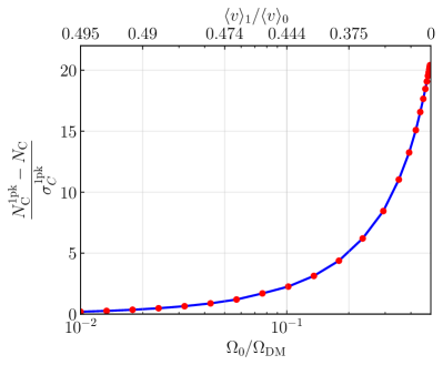
Figure 9: The difference between the cluster-number count $N_{\rm C}^{1{\rm pk}}$ obtained for $g_{v}(v)$ distribution with a single Gaussian peak and the count $N_{\rm C}$ obtained for a $g_{v}(v)$ distributions of the form given in given by Eq. (13), normalized to the the Poisson uncertainty $\sigma_{\rm C}^{1{\rm pk}}$ associated with the single-peak distribution, shown as a function of $\Omega_{0}/\Omega_{\rm DM}$ for fixed $k_{\rm FSH}\approx 0.76~{}h/\mathrm{Mpc}$. The value of $\langle v_{1}\rangle/\langle v_{0}\rangle$ which corresponds to a given value of $\Omega_{0}/\Omega_{\rm DM}$ along this $k_{\rm FSH}$ contour is indicated along the top axis. We note that $N_{\rm C}<N_{\rm C}^{1{\rm pk}}$

The results displayed in Fig. 9 clearly indicate that the detailed shape of $g_{v}(v)$ can have a significant impact on cluster-number counts. The most significant deviation occurs along the portion of the $k_{\rm FSH}$ contour where $\Omega_{0}/\Omega_{\rm DM}$ is large and $\langle v_{1}\rangle/\langle v_{0}\rangle$ is small. Indeed, this portion of the contour corresponds to the region of parameter space in Fig. 8 within which the greatest deviations likewise arose between the value of $N_{\rm SH}$ for our double-peak $g_{v}(v)$ distributions and the expected value for a WDM distribution with the same nominal free-streaming scale.

To summarize the results of this section, we find that the detailed shape of the primordial dark-matter velocity distribution not only affects the halo-mass function, but also has an impact on observables such as $N_{\rm SH}$ and $N_{\rm C}$. Thus, these observables can play a role in probing and constraining $g_{v}(v)$ and the halo- or subhalo-mass functions which follow from it.

VI A Reconstruction Conjecture

In Sect. III, we examined the mathematical relationship between $g_{M}(M)$ and $S^{2}(M)$ in the extended Press-Schechter formalism. In doing so, we identified a pair of physical thresholds which underpin this relationship. The presence of these thresholds permits us to construct a map between $v$ and $M$ analogous to the expression in Eq. (27) for any well-behaved functional forms for $W(k,R)$ and $\eta(M)$. Moreover, in Sect. V, we also saw that this relationship between $g_{M}(M)$ and $S^{2}(M)$ is such that the detailed shape of the dark-matter velocity distribution has a potentially measurable impact on astrophysical observables such as cluster-number counts.

Motivated by these findings, we propose a method for inverting the procedure outlined in Sect. III and reconstructing the detailed shape of $g_{v}(v)$ directly from information contained in $S^{2}(M)$. This conjecture is clearly more speculative than the results we have presented thus far. Indeed, it is more sensitive to the particular functional forms one chooses for $W(k,R)$ and $\eta(M)$. Moreover, the fact that the halo-mass function is not directly measurable, but rather must itself be inferred indirectly from observational data, imposes some restrictions on its practical applicability. Nevertheless, as we shall argue below, this reconstruction conjecture can provide a potentially useful method of extracting information about the primordial velocity distribution of the dark matter, and by extension the underlying particle-physics processes which produced it in the early universe.

VI.1 Formulating the Conjecture

Our stated goal, then, is to invert Eq. (31) and obtain information about $g_{M}(M)$ from $S^{2}(M)$. We begin by considering the case in which the features in $g_{M}(M)$ are well clustered in $M$-space. In this case, a statement about the functional form of $g_{M}(M)$ may then be obtained in a straightforward manner from Eq. (31). Taking the logarithmic derivative of both sides of this relation and using the definition of the hot-fraction function in Eq. (30) to relate $dF(M)/dM$ to $g_{M}(M)$, we find that

$$\frac{g_{M}(M)}{{\cal N}}~{}\approx~{}\sqrt{\frac{5}{14}}\left(\frac{d\log S^{2}(M)}{d\log M}\right)^{-1/2}\,\left|\frac{d^{2}\log S^{2}(M)}{(d\log M)^{2}}\right|~{}.$$ (41)

This is the basic form of our conjecture which allows us to reconstruct the salient features of the dark-matter velocity distribution $g_{M}(M)$ directly from the first and second logarithmic derivatives of the structure-suppression function.

As stated above, our conjecture in Eq. (41) holds under the assumption that $d^{2}\log\,S^{2}(M)/(d\log M)^{2}$ is always either zero or negative — i.e., that $\log\,S^{2}(M)$ is always either a straight line or concave-down when plotted versus $\log\,M$. However, this conjecture may also be extended to the more general case in which this condition is not always satisfied. Indeed, while we have seen in Sect. IV that $\log\,S^{2}(M)$ can in fact be concave-up, we have also seen that this behavior only arises within intervals of $M$-space within which $g_{M}(M)$ is negligible. Thus, in order to generalize our reconstruction conjecture to account for this possibility, we need only to posit that $g_{M}(M)\approx 0$ whenever $d^{2}\log\,S^{2}(M)/(d\log\,M)^{2}>0$. In other words, we posit that

$$\frac{g_{M}(M)}{{\cal N}} ~{}\approx~{} \sqrt{\frac{5}{14}}\left(\frac{d\log S^{2}(M)}{d\log M}\right)^{-1/2}$$ (42)

$$~{}~{}~{}\times\left|\min\left(0,\frac{d^{2}\log S^{2}(M)}{(d\log M)^{2}}\right)\right|~{}.~{}~{}~{}$$

This, then, is the complete statement of our reconstruction conjecture.

Several important caveats must be borne in mind regarding this conjecture. First, we emphasize that it is not meant to be a precise mathematical statement. Indeed, given the rather complicated nature of the Einstein-Boltzmann evolution equations which connect $g_{M}(M)$ to $S(M)$, we do not expect a relation of the simple form in Eq. (42) to provide a precise inverse (except perhaps under some limiting approximations and simplifications). Rather, this conjecture is intended merely as an approximate practical guide — a back-of-the-envelope method for reproducing the rough characteristics of $g_{M}(M)$ given a particular structure-suppression function $S(M)$.

Second, as discussed in more detail in Sect. II, our map between $v$ and $M$ in Eq. (27) has been formulated under the assumption that the dark matter is relativistic at the time at which it is produced. When this is not the case, we expect that a more appropriate map between these two variables will depend on further details such as the time at which the dark matter is produced, and hence will carry a sensitivity to the particular dark-matter production scenario envisaged. However, in the vast majority of situations in which this assumption is violated and a significant population of dark-matter particles is non-relativistic at the time of production, this population of non-relativistic dark-matter particles is typically sufficiently cold that it has no effect on $S^{2}(M)$ for $M$ within our regime of interest. While it is possible to engineer situations in which the map in Eq. (27) might require modification while free-streaming effects on $S^{2}(M)$ are non-negligible, such situations require a somewhat unusual dark-matter cosmology — a cosmology in which a significant non-relativistic yet “lukewarm” population of dark-matter particles is generated at exceedingly late times by some dynamics that contributes significantly to $f(v)$ within a particular range of velocities.

Third, our procedure for calculating $P(k)$ from a given $g_{v}(v)$ implicitly incorporates certain assumptions. One of these assumptions is that the background cosmology does not deviate significantly from that of the standard cosmology. For example, it is assumed that the time $t_{\mathrm{MRE}}$ of matter-radiation equality is the same as in the standard cosmology and that the universe is effectively radiation-dominated at all times from the end of the reheating epoch until $t_{\mathrm{MRE}}$. It is also assumed that the primordial spectrum of density perturbations produced after inflation is Gaussian-random. Another of these assumptions is that the velocity distribution of dark-matter particles has ceased evolving, except as a consequence of redshifting effects, by some very early time deep within the radiation-dominated epoch. This implies not only that the production of the dark matter is effectively complete by that time, but also that the effect of scattering and decay processes involving dark-matter particles is negligible thereafter. Of course, the above assumptions do not necessarily imply limitations on our conjecture per se in these regimes. While it is possible that our conjecture ceases to provide accurate results for cosmological histories wherein the above assumptions are relaxed, it is also possible that our conjecture remains robust even in the presence of these deviations.

The restrictions implied by these caveats are not severe. Indeed, as we shall demonstrate in Sect. VI.2, our conjecture as stated here will still allow us to resurrect the salient features of $g_{M}(M)$ — and hence also of $f(v)$ — for a wide variety of different dark-sector scenarios. Clearly, details such as the proportionality constants in Eq. (27) and the precise functional relationship between $d\log S^{2}(M)/d\ln M$ and $F(M)$ depend on the particular functional forms for $W(k,R)$ and $\eta(M)$. However, the qualitative picture that we have developed for reconstructing $g_{M}(M)$ from $S^{2}(M)$ is predicated only on one crucial assumption — the assumption of locality which follows from the physical thresholds which have allowed us to formulate the map between $v$ to $M$ in Eq. (27). Thus, a reconstruction conjecture qualitatively similar to Eq. (42) can likewise be formulated for any alternative functional forms that one might adopt for $W(k,R)$ and $\eta(M)$, provided that these functions respect the same thresholds. It is also worth emphasizing that, as a consequence of this locality, our reconstruction procedure permits us to reconstruct the value of $g_{M}(M)$ at any particular $M$ solely based on information about $S^{2}(M)$ and its derivatives at that same value of $M$ without any additional information about the global properties of this structure-suppression function. Thus, even if the functional form of $S^{2}(M)$ is known only across a limited range of halo masses, our conjecture can still be applied in order to reconstruct $g_{M}(M)$ across that same range of $M$.

It is also important to note the similarities and differences between our conjecture for reconstructing $f(v)$ from the shape of $S^{2}(M)$ and the similar proposal that we advanced in Ref. [5] for extracting information about the dark-matter phase-space distribution from the linear matter power spectrum [5]. First, as emphasized in the Introduction, the conjecture in Eq. (42) does not rely on this previous proposal in any way. Moreover, in principle, the conjecture in Eq. (42) permits one to extract information about $f(v)$ at much lower velocities. Measurements of $P(k)$ based on data obtained at low redshifts are currently reliable up to around $k\lesssim 0.05$ – $0.1\mbox{~{}Mpc}^{-1}$. Information from Lyman-$\alpha$-forest measurements can provide additional information about $P(k)$ at wavenumbers up to around $k\sim 1\mbox{~{}Mpc}^{-1}$. While future measurements of the 21-cm line of neutral hydrogen could in principle yield information about $P(k)$ at significantly higher redshifts, the present state of our knowledge of $P(k)$ permits us to reconstruct $f(v)$ only down to $v\sim 5\times 10^{-7}$ using the methods of Ref. [5].

By contrast, our reconstruction conjecture in Eq. (42) relies solely on information contained within the halo-mass function in order to reconstruct $f(v)$. Thus, one could in principle use this conjecture to probe $f(v)$ down to $v\sim 10^{-9}$ or lower. In practice, exploiting this property of the conjecture is somewhat challenging, given that astrophysical observables from which meaningful information about the structure-suppression function can currently be extracted, such as differential cluster-number counts, typically provide information about $S^{2}(M)$ at halo-mass scales $M\gtrsim 10^{13}~{}M_{\odot}$ — and thus to regions of $g_{v}(v)$ wherein $v\gtrsim 10^{-6}$. Nevertheless, if observational techniques can be developed which permit one to probe $S^{2}(M)$ in a meaningful way at lower scales, our reconstruction conjecture can provide a method of extracting meaningful information about the dark-matter velocity distribution from those measurements.

VI.2 Testing the Conjecture

Having stated our conjecture, we now assess the extent to which it enables us to reconstruct the underlying dark-matter velocity distribution from the halo-mass function. In particular, we shall test this conjecture within the context of an illustrative dark-matter model in which $g_{M}(M)$ deviates significantly from that of purely cold dark matter in a variety of ways within different regions of model-parameter space. For a set of illustrative points in that parameter space, we will then reconstruct $g_{M}(M)$ using our conjecture and compare it with the corresponding “true” $g_{M}(M)$ distribution.

The model which we shall adopt for purposes of illustration — a model which was introduced in Ref. [5] — is one in which the cosmological abundance of dark matter is generated non-thermally, via the decays of unstable dark-sector particles. The dark sector in this scenario consists of an ensemble of $N$ real scalar fields $\phi_{\ell}$ with $\ell=0,1,2,\ldots,N-1$ whose decay widths are dominated by two-body processes associated with trilinear terms in the interaction Lagrangian of the form

$$\mathcal{L}_{\rm int}~{}\ni~{}\sum_{\ell=0}^{N}\sum_{i=0}^{\ell}\sum_{j=0}^{i}c_{\ell ij}\phi_{\ell}\phi_{i}\phi_{j}~{},~{}$$ (43)

where the $c_{\ell ij}$ are coupling constants with dimensions of mass. The masses of the $\phi_{\ell}$ are given by $m_{\ell}=(2\ell+1)m_{0}$, where $m_{0}$ is the mass of $\phi_{0}$, while these coupling constants are given by

$$c_{\ell ij}~{} = ~{}\mu R_{\ell ij}\left(\frac{m_{\ell}-m_{i}-m_{j}}{2m_{0}}\right)^{r}\left(1+\frac{|m_{i}-m_{j}|}{2m_{0}}\right)^{s}$$ (44)

$$~{}\times~{}\Theta(m_{\ell}-m_{i}-m_{j})~{},~{}$$

where $\mu$ is a parameter with dimensions of mass, where $\Theta(x)$ denotes the Heaviside function, and where

$$R_{\ell ij}~{}=~{}\begin{cases}6&\mbox{all indices different}\\ 3&\mbox{only two indices equal}\\ 1&\mbox{all indices equal}\end{cases}$$ (45)

is a combinatorial factor. In what follows, for concreteness, we take $\mu=m_{0}/10$.

Physically, the parameter $r$ appearing in Eq. (44) governs the manner in which the $c_{\ell ij}$ scale with the overall kinetic energy released during the decay process. Taking $r>0$ establishes a preference for highly exothermic decays in which a substantial fraction of the initial mass energy $m_{\ell}$ of the decaying particle is converted into kinetic energy, while taking $r<0$ establishes a preference for decays in which a comparatively small fraction of $m_{\ell}$ is converted to kinetic energy. By contrast, the parameter $s$ governs the manner in which the $c_{\ell ij}$ scale with the difference in mass $|m_{i}-m_{j}|$ between the two daughter particles. Taking $s>0$ establishes a preference for decays in which $m_{i}$ and $m_{j}$ are very similar, while taking $s<0$ establishes a preference for decays with a significant difference between these two daughter-particle masses. Thus, by varying the parameters of this model — and in particular, by varying $r$ and $s$ — we are able to realize a variety of qualitatively different dark-matter velocity distributions in a straightforward way.

For any given choice of model parameters, we evaluate the resulting dark-matter velocity distribution $g_{v}(v)$ by numerically solving the coupled system of Boltzmann equations for the $\phi_{\ell}$. We then determine the linear matter power spectrum $P(k)$ for this $g_{v}(v)$ distribution and the linear matter power spectrum $P_{\rm CDM}(k)$ for purely cold dark matter numerically using CLASS.  We obtain $dn/d\log M$ and $(dn/d\log M)_{\rm CDM}$ from the corresponding matter power spectra using the Press-Schechter formalism, as encapsulated in Eq. (21), and use these results to construct the structure-suppression function $S^{2}(M)$. We then test our conjecture by using it to reconstruct $g_{M}(M)$ from $S^{2}(M)$, and assess how well this reconstructed $g_{M}(M)$ matches the $g_{M}(M)$ test function that we obtain from our original $g_{v}(v)$ function through use of the functional map in Eq. (27).

In Fig. 10, we display the results of our analysis for nine different combinations of the model parameters $r$ and $s$. These parameter combinations have been chosen such that the corresponding dark-matter velocity distributions exhibit a wide variety of profiles. The blue curve displayed in each panel represents the “true” velocity distribution $g_{M}(M)$ for the corresponding choice of model parameters. Indeed, we see that the set of $g_{M}(M)$ functions obtained for this set of parameter combinations includes unimodal distributions as well as a variety of multi-modal distributions. Thus, the velocity distributions shown in Fig. 10 collectively provide a thorough “stress test” of how well our conjecture performs when applied to qualitatively different kinds of dark-matter scenarios.

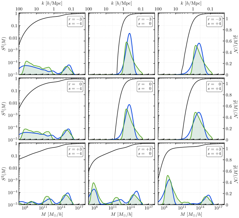
Figure 10: An explicit test of our reconstruction conjecture for a variety of different dark-matter phase-space distributions $g_{M}(M)$ which arise in the context of our illustrative dark-matter model — a model in which the dark matter is produced non-thermally through decay cascades within an extended dark sector. These distributions correspond to different choices of the parameters $r$ and $s$ in Eq. (44). Some of these distributions are unimodal, some are bi-modal, and some exhibit even more complex configurations of peaks and troughs. The blue curve shown in each panel represents the original dark-matter velocity distribution $g_{M}(M)$. The black curve represents the corresponding structure-suppression function $S^{2}(M)$ to which it gives rise. The green curve represents the reconstruction of $g_{M}(M)$ from $S^{2}(M)$ using in Eq. (42). In all cases, we see that our conjecture successfully reproduces the salient features of the original velocity distribution.

The black curve appearing in each panel of Fig. 10 represents the structure-suppression function $S^{2}(M)$ which corresponds to the velocity distribution $g_{M}(M)$. The green curve, on the other hand, represents the reconstructed $g_{M}(M)$ obtained solely from information contained in $S^{2}(M)$ using Eq. (42). In performing this test, we have chosen the value of the proportionality constant in Eq. (27) to be $\xi=9/4$, as this tends to horizontally align the original and reconstructed dark-matter velocity distributions with each other.

We observe that in each case shown, our reconstruction conjecture indeed reproduces the salient features of the original velocity distribution. In particular, we see that our conjecture allows us to reconstruct not only the approximate locations of the peaks in $g_{M}(M)$, but also the relative areas under those peaks to an impressive degree of accuracy across the entire range of $M$ shown. Thus, while our conjecture of course does not reproduce the detailed shapes of the features in $g_{M}(M)$ with perfect fidelity, the results in Fig. 10 attest that the simple relation in Eq. (42) nevertheless provides a versatile tool for extracting meaningful information about the properties of the dark matter directly from the shape of the halo-mass function alone.

VII Conclusions

The dark-matter velocity distributions which arise within the context of non-minimal dark-sector scenarios can be complicated and even multi-modal. Even within the linear regime, the small-scale-structure predictions of such scenarios differ significantly from the predictions of scenarios in which $f(v)$ is relatively narrow and unimodal, such as WDM. In this paper, we have investigated how the detailed shape of the dark-matter velocity distribution impacts structure in the non-linear regime. In particular, through use of the analytic Press-Schechter formalism, we have developed an intuition as to how features present in $f(v)$ affect the halo-mass and subhalo-mass functions. We have also studied the implications of these results for observables such as the number counts of galaxy clusters and the expected number of satellites for a Milky-Way-sized galaxy. Finally, we have proposed a conjecture which can be used to reconstruct the salient features of the primordial dark-matter velocity distribution $f(v)$ directly from the shape of the halo-mass function $dn/d\log M$. This reconstruction conjecture requires essentially no additional information about the properties of the dark matter beyond what is imprinted on $dn/d\log M$ itself. Moreover, we have shown that our conjecture successfully reproduces the salient features of the underlying dark-matter velocity distribution even in situations in which that distribution is complicated and even multi-modal.

Several comments are in order. First of all, our results are predicated on a number of theoretical assumptions concerning the form of the halo-mass function, the window function $W(k,R)$, etc.  For example, in our analysis, we have adopted the functional form for $\eta(M)$ in Eq. (23). However, as discussed in Sect. III, there exist a number of alternatives we could have chosen for $\eta(M)$.  Likewise, while our choice of the window function in Eq. (19) allows us to formulate the map between $k$ and $M$ in an unambiguous way, it is certainly possible to consider alternatives for $W(k,R)$. Such modifications would of course have an impact on our quantitative results for $S^{2}(M)$, $N_{\rm SH}$, and $N_{\rm C}$, as well as the precise form of the empirical relation between $d\log S^{2}(M)/d\log M$ and $F(M)$ in Eq. (31). However, for well-behaved window functions — i.e., functions which have sufficiently flat tops and which decay sufficiently rapidly for $k\gtrsim R^{-1}$ — we expect that these modifications will not alter the qualitative nature of our results, including the fundamental relationship between $d\log S^{2}(M)/d\log M$ and $F(M)$ which underlies the reconstruction conjecture in Eq. (42). This issue merits further exploration.

One interesting feature of our analysis is that it makes no particular assumption about the masses of the individual dark-matter particles themselves. As such, this analysis is applicable not only to the case in which $g_{v}(v)$ receives contributions from a single dark-matter species with a well-defined mass, but also to the case in which multiple particle species contribute to the present-day dark-matter abundance (an extreme example of which occurs in the Dynamical Dark Matter framework [48, 49]). The corresponding distribution $g_{v}(v)$ in this latter case represents the aggregate velocity distribution for all particle species which contribute to the present-day dark-matter abundance. Of course, this also means that while observables such as $N_{\rm SH}$ and $N_{\rm C}$ are sensitive to the detailed shape of $g_{v}(v)$, they are not capable of distinguishing between single-particle and multi-particle dark-matter scenarios which yield the same $g_{v}(v)$ distribution.

We also note that we have assumed throughout this paper that the dark matter has negligible self-interactions. Indeed, if dark-matter self-interactions were sufficiently strong, the the shape of $g_{v}(v)$ would continue to evolve at times $t>t_{\rm MRE}$. It would be interesting to explore how the presence of appreciable dark-matter self-interactions would affect our results.

While we have focused in this paper primarily on the halo-mass function $dN/d\log M$, we also note that the subhalo-mass function — i.e., the differential number of subhalos $dN_{\rm SH}/d\log M$ within a host halo of mass $M_{0}$ — also provides an observational handle on the detailed shape of $g_{v}(v)$. Indeed, we have already seen in Sect. V.1 that even the integral number of subhalos $N_{\rm SH}$ within a given host halo can provide such a handle. Strong gravitational lensing provides a tool which can be used to probe this subhalo-mass function on mass scales $M\sim 10^{6}$ – $10^{8}$ $M_{\odot}$. Analyses of small existing samples of strongly-lensed objects have already yielded meaningful constraints on the subhalo-mass function [50, 51, 52]. Moreover, a significant number of additional strong-lensing candidates have been identified within SDSS data [53]. It would be interesting to consider how $dN_{\rm SH}/d\log M$ depends on $g_{v}(v)$ for different $M_{0}$. It would also be interesting to consider whether a procedure could be developed for reconstructing $g_{M}(M)$ from the shape of $dN_{\rm SH}/d\log M$ at scales $M\lesssim 10^{10}~{}M_{\odot}$.

As noted in Sect. VI, the reconstruction conjecture we have formulated in Eq. (42) has two distinct components: first, the assertion that the hot-fraction function $F(k)$ is connected to the slope of the structure-suppression function, and second, that this relation takes the explicit form in Eq. (31). Indeed, these two assertions together yield our final conjecture in Eq. (42). As evident in Fig. 10, our conjecture is remarkably successful in reproducing the salient features of $g_{M}(M)$. However, just as with the conjecture presented in Ref. [5], we regard this conjecture as at best purely empirical. It is therefore possible that one or both aspects of this conjecture might be further refined. For example, it is possible that the hot-fraction function $F(M)$ might also carry a weak dependence on other (higher) derivatives of the structure-suppression function, or on the value of the structure-suppression function itself. Likewise, even with this assumption, it is possible that the relation in Eq. (31) might carry higher-order corrections. Although it is not possible to rigorously invert the mathematical procedure discussed in Sect. III through which a given dark-matter velocity distribution $g_{v}(v)$ produces a corresponding structure-suppression function $S(M)$, it may be possible to trace through such a calculation analytically to leading order and thereby determine which features of $g_{v}(v)$ might dominate the resulting $S^{2}(M)$ and vice versa. In this way, one might hope to eventually derive our conjecture analytically, along with possible correction terms.

On the surface, the problem of reconstructing of $g_{M}(M)$ from $S^{2}(M)$ bears similarity to another well-known inverse problem in kinetic theory, namely the determination of the phase-space distribution $f(p)$ of a gas of particles from quantities which depend on $f(p)$ only through the moments of this distribution. While it is generally possible to solve this inverse problem, the procedure for doing so typically yields a significant number of mathematically consistent solutions — solutions which may or may not be physically sensible. The reason why our reconstruction conjecture does not give rise to a similarly large multiplicity of solutions is ultimately that the relationship between the $g_{M}(M)$ and $S^{2}(M)$ is local in the sense that the value of $g_{M}(M)$ at any particular value of $M$ depends only on the value of $S^{2}(M)$ and its derivatives at that same value of $M$. As a result of this locality, our reconstruction conjecture gives us access to $g_{M}(M)$ directly, rather than requiring us to infer the shape of this distribution from its moments.

Our reconstruction conjecture in principle provides a method of obtaining information about the dark-matter velocity distribution from the shape of the halo-mass function. Of course, the practical utility of this procedure depends on our ability to determine the shape of the halo-mass function, which is itself not a directly measurable quantity. Doing this presents its own set of challenges. Significant theoretical uncertainties exist in the relationship between the relevant astrophysical observables and halo mass. Moreover, statistical fluctuations in the measured values of these observables can introduce a so-called Eddington bias [54]. Furthermore, the accuracy to which the mass of an individual halo can be measured is limited both by the number density of background source images and by uncertainties in the shapes of foreground halos.

Nevertheless, despite these challenges, strides have been made toward extracting information about the halo-mass function from observation. In particular, methods have been proposed for obtaining information about $dn/d\log M$ from cosmic-microwave-background (CMB) data [55], galaxy-cluster number counts [11], weak lensing of the CMB [56] and other background sources [12, 13], the line widths of neutral hydrogen emitted by galaxies [14], and the foreground-background galaxy angular cross-correlation function in conjunction with with background samples of sub-millimeter galaxies [15]. Such methods make no assumptions about the primordial dark-matter velocity distribution $f(v)$, which it is the aim of our conjecture to extract. Moreover, while many of these methods yield information about $dn/d\log M$ only at scales $M\gtrsim 10^{13}~{}M_{\odot}$, others others are in principle capable of probing the halo-mass function down to $M\sim 10^{10}~{}M_{\odot}$. Empirical models relating the luminosities of galaxies to the masses of their host halos [57, 58, 59, 60] can also potentially be used in conjunction with observation in order to provide meaningful information about $dn/d\log M$. However, since these models are predicated on the assumption that the dark-matter velocity distribution takes a particular, simple form, significant numerical work would be required in order to assess their applicability to scenarios with significantly more complicated $g_{v}(v)$ distributions. Thus, despite the challenges involved in determining the halo-mass function from observation, larger data sets and an improved understanding of the theoretical relationship between astrophysical observables and halo mass could significantly reduce the uncertainties in $dn/d\log M$ in the near future. As such, a calculational tool of the sort we have proposed in this paper could potentially be a valuable addition to the toolbox of the dark-matter cosmologist.