Regularization by dynamic programming

Abstract

We investigate continuous regularization methods for linear inverse problems of static and dynamic type. These methods are based on dynamic programming approaches for linear quadratic optimal control problems. We prove regularization properties and also obtain rates of convergence for our methods. A numerical example concerning a dynamical electrical impedance tomography (EIT) problem is used to illustrate the theoretical results.

1 Introduction

We begin by introducing the notion of dynamic inverse problems. Roughly speaking, these are inverse problems in which the measuring process –performed to obtain the data– is time dependent. As usual, the problem data corresponds to indirect information about an unknown parameter, which has to be reconstructed. The desired parameter is allowed to be itself time dependent.

Let $X$, $Y$ be Hilbert spaces. We consider the inverse problem of finding $u:[0,T]\to X$ of the system

$$F(t)u(t)\ =\ y(t)\,,\ t\in[0,T]\,,$$ (1)

where $y:[0,T]\to Y$ are the dynamic measured data and $F(t):X\to Y$ are linear ill-posed operators indexed by the parameter $t\in[0,T]$. Notice that $t\in[0,T]$ corresponds to a (continuous) temporal index. The linear operators $F(t)$ map the unknown parameter $u(t)$ to the measurements $y(t)$ at the time point $t$ during the finite time interval $[0,T]$. We shall refer to (1) as dynamic inverse problem.

Since the operators $F(t)$ are ill-posed, at each time point $t\in[0,T]$ the solution $u(t)$ does not depend on a stable way on the right hand side $y(t)$. Therefore, regularization techniques have to be used in order to obtain a stable solution $u(t)$. In this article we consider time dependent regularization methods [11], which take into account the fact that the parameter $u(t)$ evolves continuously with the time.

If the measuring process is stationary and the parameter is not time dependent, the dynamic inverse problem (1) reduces to the standard problem of finding a solution $u\in X$ of the equation

$$Fu\ =\ y\,,$$ (2)

where $F:X\to Y$ is a linear ill-posed parameter to output operator and $y\in Y$. In opposition to (1) we shall refer to (2) as static inverse problem.

The second main goal in this article is to investigate continuous regularization methods [22] for the inverse problem (2). The regularization methods proposed for problems (1) and (2) are related by the fact that both of them derive from a solution technique for linear quadratic optimal control problems [5], the so-called dynamic programming [2, 3, 4].

Some relevant applications

As a first example of dynamic inverse problem, we present the dynamical source identification problem: Let $u(x,t)$ be a solution to

$$\Delta_{x}u(x,t)=f(x,t)\quad\mbox{ in }\Omega,$$

where $f(x,t)$ represents an unknown source which moves around and might change shape with time $t$. The inverse problem in this case is to reconstruct $f$ from single or multiple measurements of Dirichlet and Neumann data $(u(x,t)$, $\partial_{n}u(x,t))$, on the boundary $\partial\Omega$ over time $t\in[0,T]$. Such problems arise in the field of medical imaging, e.g. brain source reconstruction [1] or electrocardiography [16].

Many other ’classical’ inverse problems have corresponding dynamic counterparts, e.g., the dynamic electrical impedance tomography problem consists in reconstructing the time-dependent diffusion coefficient (impedance) in the equation

$$\nabla_{x}\cdot(\sigma(.,t)\nabla_{x})u(.,t)\ =\ 0,$$ (3)

from measurements of the time-dependent Dirichlet to Neumann map $\Lambda_{\sigma}$ (see the review paper [6]). This problem can model a moving object with different impedance inside a fluid with uniform impedance, for instance the heart inside the body. Notice that in this case we assume the time-scale of the movement to be large compared to the speed of the electro-magnetic waves. Hence, the quasi-static formulation (3) is a valid approximation for the physical phenomena.

Another application concerning dynamical identification problems for the heat equation is considered in [14, 15]. Other examples of dynamic inverse problems can be found in [19, 21, 23, 24, 25]. In particular, for applications related to process tomography, see the conference papers by M.H.Pham, Y.Hua, N.B.Gray; M.Rychagov, S.Tereshchenko; I.G.Kazantsev, I.Lemahieu in [18].

Literature overview and outline of the paper

Continuous and discrete regularization methods for static inverse problems have been quite well studied in the last two decades and one can find relevant information, e.g., in [7, 8, 9, 10, 17, 22] and in the references therein.

What concerns dynamic inverse problems, regularization methods were considered for the first time in [20, 21]. There, the authors analyze discrete dynamic inverse problems and propose a procedure called spatio temporal regularizer (STR), which is based on the minimization of the functional

$$\Phi(u)\ :=\ \textstyle\sum\limits_{k=0}^{N}\|F_{k}u_{k}-y_{k}\|_{L^{2}}^{2}+\lambda^{2}\textstyle\sum\limits_{k=0}^{N}\|u_{k}\|_{L^{2}}^{2}+\mu^{2}\textstyle\sum\limits_{k=0}^{N-1}\frac{\|u_{k+1}-u_{k}\|_{L^{2}}^{2}}{(t_{k+1}-t_{k})^{2}}.$$ (4)

Notice that the term with factor $\lambda^{2}$ corresponds to the classical (spacial) Tikhonov-Philips regularization, while the term with factor $\mu^{2}$ enforces the temporal smoothness of $u_{k}$.

A characteristic of this approach is the fact that the hole solution vector $\{u_{k}\}_{k=0}^{N}$ has to be computed at a time. Therefore, the corresponding system of equations to evaluate $\{u_{k}\}$ has very large dimension. In the STR regularization, the associated system matrix is decomposed and rewritten into a Sylvester matrix form. The efficiency of this approach is based on fast solvers for the Sylvester equation.

In [11] continuous and iterative regularization methods based on dynamic programming techniques were proposed as an alternative for obtaining stable solutions of (1). In this article the authors verify regularization properties of the proposed methods and present numerical realizations for a dynamic electrical impedance tomography (EIT) problem, similar to the one treated in [21].

A word about the coupling of inverse problems and dynamic programming theory. So far this theory have been mostly applied to solve particular inverse problems. In [14] the inverse problem of identifying the initial condition in a semilinear parabolic equation is considered. In [15] the same authors consider a problem of parameter identification for systems with distributed parameters. In [12], the dynamic programming methods are used in order to formulate an abstract functional analytical method to treat static inverse problems (2).

This paper is outlined as follows: In Section 2 we derive the solution methods discussed in this paper. In Section 3 we analyze some regularization properties of the proposed methods. In Section 4 we present numerical realizations of the discrete regularization method as well as a discretization of the continuous regularization method. For comparison purposes we consider a dynamic EIT problem, similar to the one treated in [21].

2 Derivation of the regularization methods

2.1 Static inverse problems

We start this subsection defining an optimal control problem related with the linear inverse problem (2). Let $u_{0}\in X$ be any approximation for the minimum norm solution $u^{\dagger}\in X$ of (2). We aim to find a function $u:[0,T]\to X$ such that, $u(0)=u_{0}$ and

$$\|Fu(T)-y\|\ \approx\ \|Fu^{\dagger}-y\|\,.$$ (5)

In the control literature, the function $u$ is called trajectory (or state) and its evolution is is described by a dynamical system. For simplicity, we choose a linear evolution model, i.e. $u^{\prime}=Au(t)+Bv(t)$, $t\geq 0$, where $A,B:X\to X$ are linear operators and $v:[0,T]\to X$ is the control of the system. Since our main concern is to satisfy the property in (5), it is enough for our purpose to consider a simpler dynamic, which does not depend on the state $u$, but only on the control $v$ (for a dynamic including the state see [13]). This justifies the choice of the dynamic: $u^{\prime}=v$, $t\geq 0$. In this case, the control $v$ corresponds to a velocity function.

The next step is to choose the objective function for our control problem. The following choice is related to the minimization of both the residual norm and the velocity norm along the trajectories

$$J(u,v):=\textstyle\frac{1}{2}\displaystyle\int_{0}^{T}\|Fu(t)-y\|^{2}+\|v(t)\|^{2}\ dt.$$

Putting all together we obtain the following abstract optimal control problem in Hilbert spaces:

$$\left\{\begin{array}[]{l}{\rm Mimimize}\ J(u,v)=\frac{1}{2}\displaystyle\int_{0}^{T}\|Fu(t)-y\|^{2}+\|v(t)\|^{2}\ dt\\ {\rm s.t.}\\ u^{\prime}=v,\ t\geq 0,\ \ u(0)=u_{0}\,,\end{array}\right.$$ (6)

where the (fixed but arbitrary) final time $T>0$ will play the role of the regularization parameter. The functions $u,v:[0,T]\to X$ correspond respectively to the trajectory an the control of the system, and the pairs $(u,v)$ are called processes.

Next we define the residual function $\varepsilon(t):=Fu(t)-y$ associated to a given trajectory $u$. Notice that this residual function evolves according to the dynamic

$$\varepsilon^{\prime}=Fu^{\prime}(t)=Fv(t)\,,\ t\geq 0\,.$$

With this notation, problem (6) can be rewritten in the following form

$$\left\{\begin{array}[]{l}{\rm Mimimize}\ J(\varepsilon,v)=\frac{1}{2}\displaystyle\int_{0}^{T}\|\varepsilon(t)\|^{2}+\|v(t)\|^{2}\ dt\\ {\rm s.t.}\\ \varepsilon^{\prime}=Fv,\ t\geq 0,\ \ \varepsilon(0)=Fu_{0}-y\,.\end{array}\right.$$ (7)

In [12, Proposition 2.1] the equivalence between the solvability of the optimal control problem (6) and the auxiliary problem (7) is established. In the sequel, we derive the dynamic programming approach for the optimal control problem in (7). We start by introducing the first Hamilton function. This is the function $H:\mathbb{R}\times X^{3}\to\mathbb{R}$ given by

$$H(t,\varepsilon,\lambda,v)\ :=\ \displaystyle\langle\lambda,Fv\rangle+\textstyle\frac{1}{2}\displaystyle[\langle\varepsilon,\varepsilon\rangle+\langle v,v\rangle]\,.$$

Notice that the variable $\lambda$ plays the role of a Lagrange multiplier in the above definition. According to the Pontryagin’s maximum principle, the Hamilton function furnishes a necessary condition of optimality for problem (7). Furthermore, since this function (in this particular case) is convex in the control variable, this optimality condition also happens to be sufficient. Recalling the maximum principle, along an optimal trajectory we must have

$$0\ =\ \frac{\partial H}{\partial v}(t,\varepsilon(t),\lambda(t),v(t))\ =\ F^{*}\lambda(t)+v(t)\,.$$ (8)

This means that the optimal control $\bar{v}$ can be obtained directly from the Lagrange multiplier $\lambda:[0,T]\to X$, by the formula

$$\bar{v}(t)=-F^{*}\lambda(t)\,,\ \forall t\,.$$

Therefore, the key task is actually the evaluation of the Lagrange multiplier. This leads us to the Hamilton-Jacobi equation. Substituting the above expression for $\bar{v}$ in (8), we can define the second Hamilton function $\mathcal{H}:\mathbb{R}\times X^{2}\to\mathbb{R}$

$$\mathcal{H}(t,u,\lambda)\ :=\ \min_{v\in X}\{H(t,\varepsilon,\lambda,v)\}\ =\ \textstyle\frac{1}{2}\displaystyle\langle\varepsilon,\varepsilon\rangle-\textstyle\frac{1}{2}\displaystyle\langle\lambda,FF^{*}\lambda\rangle\,.$$

Now, let $V:[0,T]\times X\to\mathbb{R}$ be the value function for problem (7), i.e.

$$V(t,\xi)\!\!\! := \!\!\!\min\Big{\{}\textstyle\frac{1}{2}\int_{t}^{T}\|\varepsilon(s)\|^{2}+\|v(s)\|^{2}\,ds\ \Big{|}\ (\varepsilon,v)\ {\rm admissible\ process}$$ (9)

$$\!\!\!{\rm\ \ \ \ \ \ \ \ for\ problem\ (\ref{eq:ccpr-hs})\ with\ initial\ condition}\ \varepsilon(t)=\xi\Big{\}}\,.$$

The interest in the value function follows from the fact that this function is related to the Lagrange multiplier $\lambda$ by the formula: $\lambda(t)=\partial V/\partial\varepsilon(t,\bar{\varepsilon})$, where $\bar{\varepsilon}$ is an optimal trajectory.

From the control theory we know that the value function is a solution of the Hamilton-Jacobi equation

$$\frac{\partial V}{\partial t}(t,\varepsilon)+\mathcal{H}(t,\varepsilon,\frac{\partial V}{\partial\varepsilon}(t,\varepsilon))\ =\ 0\,.$$ (10)

Now, making the ansatz: $V(t,\varepsilon)=\frac{1}{2}\langle\varepsilon,Q(t)\varepsilon\rangle$, with $Q:[0,T]\to\mathbb{R}$, we are able to rewrite (10) in the form

$$\langle\varepsilon,Q^{\prime}(t)\varepsilon\rangle+\langle\varepsilon,\varepsilon\rangle-\langle Q(t)\varepsilon,FF^{*}Q(t)\varepsilon\rangle\ =\ 0\,.$$

Since this equation must hold for all $\varepsilon\in X$, the function $Q$ can be obtained by solving the Riccati equation

$$Q^{\prime}(t)\ =\ -I+Q(t)FF^{*}Q(t)\,.$$ (11)

Notice that the cost of all admissible processes for an initial condition of the type $(T,\varepsilon)$ is zero. Therefore we have to consider the Riccati equation (11) with the final condition

$$Q(T)\ =\ 0\,.$$ (12)

Once we have solved the initial value problem (11), (12), the Lagrange multiplier is given by $\lambda(t)=Q(t)\bar{\varepsilon}(t)$ and the optimal control is obtained by the formula $\bar{v}(t)=-F^{*}Q(t)\bar{\varepsilon}(t)$. Therefore, the optimal trajectory of problem (6) is defined via

$$\bar{u}^{\prime}=-F^{*}Q(t)[F\bar{u}(t)-y]\,,\ \ \bar{u}(0)=u_{0}\,.$$ (13)

We use the optimal trajectory defined by the initial value problem (13) in order to define a family of reconstruction operators $R_{T}:X\to X$, $T\in\mathbb{R}^{+}$,

$$R_{T}(y)\ :=\ \bar{u}(T)\ =\ u_{0}-\int_{0}^{T}F^{*}Q(t)[F\bar{u}(t)-y]\ dt\,.$$ (14)

We shall return to the operators $\{R_{T}\}$ in Section 3 and prove that the family of operators defined in (14) is a regularization method for (2) (see, e.g., [7]).

2.2 Dynamic inverse problems

In the sequel we consider the dynamic inverse problem described in (1). As in the previous subsection, we shall look for a continuous regularization strategy.

We start by considering the constrained optimization problem

$$\left\{\begin{array}[]{l}{\rm Mimimize}\ J(u,v):={\textstyle\frac{1}{2}}\int_{0}^{T}\big{[}\,\langle F(t)u(t)-y(t),\ L(t)[F(t)u(t)-y(t)]\rangle\\[4.30554pt] \hskip 119.50148pt+\ \langle v(t),M(t)v(t)\rangle\,\big{]}\ dt\\[4.30554pt] {\rm s.t.}\ \ u^{\prime}=A(t)u+B(t)v(t),\ t\in[0,T],\ u(0)=u_{0}\,,\end{array}\right.$$ (15)

where $F(t)$, $u(t)$ and $y(t)$ are defined as in (1), $v(t)\in X$, $t\in[0,T]$, $L(t):Y\to Y$, $M(t):X\to X$, $A(t)\equiv I:X\to X$, $B(t)\equiv 0$ and $u_{0}\in X$.

Following the footsteps of the previous subsection, we define the first Hamilton function $H:[0,T]\times X^{3}\to\mathbb{R}$ by

$$H(t,u,\lambda,v)\ :=\ \langle\lambda,v\rangle+{\textstyle\frac{1}{2}}[\langle F(t)u-y(t),L(t)(F(t)u-y(t))\rangle+\langle v,M(t)v\rangle]\,.$$

Thus, it follows from the maximum principle: $0=\partial H/\partial v(t,u(t),\lambda(t),v(t))=\lambda(t)+M(t)v(t)$, and we obtain a relation between the optimal control and the Lagrange parameter, namely: $\bar{v}(t)=-M^{-1}(t)\lambda(t)$.

As before, we define the second Hamilton function $\mathcal{H}:\mathbb{R}\times X^{2}\to\mathbb{R}$

$$\mathcal{H}(t,u,\lambda)\,:=\,{\textstyle\frac{1}{2}}\langle F(t)u-y(t),L(t)(F(t)u-y(t)\rangle-{\textstyle\frac{1}{2}}\langle\lambda,M(t)^{-1}\lambda\rangle\,.$$

Since $\lambda(t)=\partial V/\partial u(t,u)$, where $V:[0,T]\times X\to\mathbb{R}$ is the value function of problem (15), it is enough to obtain $V$. This is done by solving the Hamilton–Jacobi (HJ) equation (see (10))

$$0 = V_{t}+{\textstyle\frac{1}{2}}\langle F(t)u-y(t),L(t)(F(t)u-y(t))\rangle-{\textstyle\frac{1}{2}}\langle V_{u},M(t)^{-1}V_{u}\rangle\,.$$

We make the ansatz $V(t,u)={\textstyle\frac{1}{2}}\langle u,Q(t)u\rangle+\langle b(t),u\rangle+g(t)$, with $Q:[0,T]\to\mathbb{R}$, $b:[0,T]\to X$ and $g:\mathbb{R}\to\mathbb{R}$. Then, we are able to rewrite the HJ equation above in the form of a polynomial equation in $u$. Moreover, the quadratic, the linear and the constant terms of this polynomial equation must all vanish. Thus we obtain

$$Q^{\prime}=Q^{*}M(t)^{-1}Q-F^{*}(t)L(t)F(t),\ \ b^{\prime}=Q(t)^{*}M(t)^{-1}b+F^{*}(t)L(t)y(t).$$ (16)

The final conditions $Q(T)=0$, $b(T)=0$ are derived just like in the previous subsection. Once the above system is solved, the optimal control $\bar{u}$ is obtained by solving

$$\bar{u}^{\prime}(t)=-M^{-1}(t)V_{u}(t,u)=-M^{-1}(t)[Q(t)\bar{u}(t)+b(t)]$$ (17)

with initial condition $\bar{u}(0)=u_{0}$.

Following the ideas of the previous tutorial subsection, we shall choose a family of operators $\{M_{\alpha},L_{\alpha}\}_{\alpha>0}$ and use the corresponding optimal trajectories $\bar{u}_{\alpha}$ in order to define a family of reconstruction operators $R_{\alpha}:L^{2}((0,T);Y)\to H^{1}((0,T);X)$,

$$R_{\alpha}(y):=u_{0}-\textstyle\int_{0}^{t}M_{\alpha}^{-1}(s)[Q(s)\bar{u}(s)+b(s)]\,ds\,.$$

The regularization properties of the operators $\{R_{\alpha}\}$ will be analyzed in Section 3.

3 Analysis of regularization properties

3.1 Static inverse problems

In this section we investigate the regularization properties of the operator $R_{T}$ introduced in (14). Consider the Riccati equation (11) for the operator $Q$: We may express the operator $Q(t)$ via the spectral family $\{F_{\lambda}\}$ of $FF^{*}$ (see e.g. [7]). Hence, we make the ansatz

$$Q(t)=\int q(t,\lambda)dF_{\lambda}\;.$$

Assuming that $q(t,\lambda)$ is $C^{1}$ we may find from (11) together with the boundary condition at $t=T$ that

$$\int\left(\textstyle\frac{d}{dt}q(t,\lambda)+1-q(t,\lambda)^{2}\lambda\right)\ dF_{\lambda}=0,\ \ \ q(T,\lambda)=0.$$

Hence, we obtain an ordinary differential equation for $q$:

$$\textstyle\frac{d}{dt}q(t,\lambda)=-1+\lambda q(t,\lambda)^{2}$$ (18)

The solution to these equations is given by

$$q(t,\lambda)=-\frac{1}{\sqrt{\lambda}}\tanh(\sqrt{\lambda}(t-T))=\frac{1}{\sqrt{\lambda}}\tanh(\sqrt{\lambda}(T-t)).$$ (19)

If $t<T$, then $Q(t)$ is nonsingular, since $\lim_{x\to 0}\frac{\tanh(xa)}{x}=a$ and $\frac{\tanh(ax)}{x}$ is monotonically decreasing for $x>0$. Hence the spectrum of $Q(t)$ is contained in the interval $[\frac{\tanh((T-t)\|F\|)}{\|F\|},(T-t)]$. Now consider the evolution equation (13): The operator $Q(t)$ can be expressed as $Q(t)=q(t,FF^{*})$; by usual spectral theoretic properties (see, e.g., [7]) it holds that

$$F^{*}q(t,FF^{*})=q(t,F^{*}F)F^{*}.$$

Hence we obtain the problem

$$u^{\prime}(t) = -q(t,F^{*}F)\left(F^{*}Fu(t)-F^{*}y\right)$$ (20)

$$u(0) = u_{0}$$ (21)

We may again use an ansatz via spectral calculus: if we set

$$u(t)=\int g(t,\lambda)dE_{\lambda}F^{*}y$$

where $E_{\lambda}$ is the spectral family of $F^{*}F$, we derive an ordinary differential equation for $g$. Similar as above, we can express the solution to (20,21) in the form

$$u(t)=\int\frac{1-\frac{\cosh(\sqrt{\lambda}(T-t))}{\cosh(\sqrt{\lambda}T)}}{\lambda}dE_{\lambda}F^{*}y+\int\frac{\cosh(\sqrt{\lambda}(T-t))}{\cosh(\sqrt{\lambda}T)}dE_{\lambda}u_{0}.$$ (22)

Setting $t=T$ we find an approximation of the solution

$$u_{T}:=u(T)=\int\frac{1-\frac{1}{\cosh(\sqrt{\lambda}T)}}{\lambda}dE_{\lambda}F^{*}y+\int\frac{1}{\cosh(\sqrt{\lambda}T)}dE_{\lambda}u_{0}.$$ (23)

Note the similarity to Showalter‘s methods [7], where the term $\exp(\lambda T)$ instead of $\cosh(\sqrt{\lambda}T)$ appears.

Theorem 3.1.

The operator $R_{T}$ in (14) is a regularization operator with qualification $\mu_{0}=\infty$:

If the data are exact, $y=Fu^{\dagger}$ and $u^{\dagger}$ satisfies a source condition for some $\mu>0$

$$\exists\ \omega\in X:\quad u^{\dagger}=(F^{*}F)^{\mu}\omega,$$ (24)

we have the estimate

$$\|u_{T}-u^{\dagger}\|\leq C_{\mu}T^{-2\mu}$$

If the data are contaminated with noise, $\|y-y_{\delta}\|\leq\delta$ and $y=Fu^{\dagger}$ with $u^{\dagger}$ as in (24), then we have

$$\|u_{T,\delta}-u^{\dagger}\|\leq C_{\mu}T^{-2\mu}+\delta T.$$

In particular, the a-priori parameter choice $T\sim\delta^{\frac{-1}{2\mu+1}}$ yields the optimal order convergence rate

$$\|u_{T,\delta}-u^{\dagger}\|\sim\delta^{\frac{2}{2\mu+1}}.$$

Proof: See [12, Theorem 3.1].

Comparing the dynamic programming approach with the Showalter method, one observes that they are quite similar, with $T_{dyn}^{2}\sim T_{Sw}$. Hence, to obtain the same order of convergence we only need $\sqrt{T_{Sw}}$ of the time for the Showalter method.

3.2 Dynamic inverse problems

Before we examine the regularization properties of the method derived in Subsection 2.2, we state a result about existence and uniqueness of the Riccati equations (16).

Theorem 3.2.

If $F$, $L$, $M\in C([0,T],\mathcal{L}(X,Y))$, then the Riccati equation (16) has a unique symmetric positive semidefinite solution in $C^{1}([0,T],\mathcal{L}(X))$.

Proof: See [11, Theorem 3.1].

Remark 3.3.

It is well known in control theory that the existence of a solution to (16) can be constructed from the functional

$$V(t,\xi):=\min_{\begin{subarray}{c}{u(t)=\xi}\\ {u\in H^{1}([t,T],X)}\end{subarray}}{\textstyle\frac{1}{2}}\textstyle\int_{t}^{T}\langle F(s)u(s)-y(s),L(s)[F(s)u(s)-y(s)]\rangle\\ +\langle u^{\prime}(s),M(s)u^{\prime}(s)\rangle ds.$$ (25)

This functional is quadratic in $u$ and, from the Tikhonov regularization theory (see, e.g., [7]), it admits a unique solution $u$, and is quadratic in $\xi$. Furthermore, the leading quadratic part $(\xi,Q(t)\xi)$ is a solution to the Riccati Equation.

Next we consider regularization properties of the method derived in Subsection 2.2. The following lemma shows that the solution $u$ of (17) satisfies the necessary optimality condition for the functional

$$J(u)\ =\ {\textstyle\frac{1}{2}}\textstyle\int_{0}^{T}\langle F(s)u(s)-y(s),L(s)[F(s)u(s)-y(s)]\rangle\\ +\langle u^{\prime}(s),M(s)u^{\prime}(s)\rangle ds$$ (26)

(notice that this is the cost functional $J(u,v)$ in (15) with $v=u^{\prime}$).

Lemma 3.4.

Let $Q(t)$, $b(t)$, $u(t)$ be defined by (16), (17), together with the boundary conditions $Q(T)=0$, $b(T)=0$ and $u(0)=u_{0}$. Then, $u(t)$ solves

$$F^{*}(t)L(t)F(t)u(t)-\left(M(t)u(t)^{\prime}\right)^{\prime}=F^{*}(t)L(t)y(t),$$ (27)

together with the boundary conditions $u(0)=u_{0}$, $u^{\prime}(T)=0$.

Proof: See [11, Lemma 3.3].

Since the cost functional in (26) is quadratic, the necessary first order conditions are also sufficient. Thus, the solution $u(t)$ of (27) is actually a minimizer of this functional. Including the boundary conditions we obtain the following corollary:

Corollary 3.5.

The solution $u(t)$ of (27) is a minimizer of the Tikhonov functional in (26) over the linear manifold

$$\mathcal{H}:=\{u\in H^{1}([0,T],X)\ |\ u(0)=u_{0}\}\,.$$

In particular, this means that the above procedure is a regularization method for the inverse problem (1). Bellow we summarize a stability and convergence result. The proof uses classical techniques from the analysis of Tikhonov type regularization methods (cf. [7], [8]) and thus is omitted.

Theorem 3.6.

Let $M(t)\equiv\alpha I$, $\alpha>0$, $L(t)>0$, $t\in[0,T]$ and $J_{\alpha}$ be the corresponding Tikhonov functional given by (26).
Stability: Let the data $y(t)$ be noise free and denote by $u_{\alpha}(t)$ the minimizer of $J_{\alpha}$. Then, for every sequence $\{\alpha_{k}\}_{k\in\mathbb{N}}$ converging to zero, there exists a subsequence $\{\alpha_{k_{j}}\}_{j\in\mathbb{N}}$, such that $\{u_{\alpha_{k_{j}}}\}_{j\in\mathbb{N}}$ is strongly convergent. Moreover, the limit is a minimal norm solution.
Convergence: Let $\|y^{\delta}(t)-y(t)\|\leq\delta$. If $\alpha=\alpha(\delta)$ satisfies

$$\lim_{\delta\to 0}\alpha(\delta)=0\mbox{ \ \ and \ \ }\lim_{\delta\to 0}\delta^{2}/\alpha(\delta)=0\,.$$

Then, for a sequence $\{\delta_{k}\}_{k\in\mathbb{N}}$ converging to zero, there exists a sequence $\{\alpha_{k}:=\alpha(\delta_{k})\}_{k\in\mathbb{N}}$ such that $u_{\alpha_{k}}$ converges to a minimal norm solution.

For the sake of completeness we also include the corresponding algorithms for the discretized dynamical case. Instead of having a continuous time variable we assume that the data and the operator are given on discrete time steps $k=1,\ldots N$. Instead of (26) a functional is used where the integrals are replaced by sums, the derivatives by differences very similar to (4). The operators $F(t)$, $L(t)$ are replaced by sequences $F_{k}$, $L_{k}$, $k=1,\ldots N$, the data $y(t)$ are now given as a sequence $y_{k}$ and instead of a time dependent solution $u(t)$ we are looking for a set of solutions $u_{k}$. The dynamic programming approach goes through in a similar manner and as a result we obtain an iterative procedure instead of the evolution equations (16), (17). The details can be found in [11, 12], we just state the iterations. Set $Q_{N+1}:=0$, $b_{N+1}:=0$ and fix an initial guess $u_{0}$. The corresponding minimizer of the discrete version of (26) can be found by two backwards iterations on $Q$ and $b$ and a forward iteration on $u$ (for simplicity we put $M=I$):

$$Q_{k-1} =(Q_{k}+\alpha^{-1}I)^{-1}Q_{k}+F_{k-1}^{*}L_{k-1}F_{k-1} k=N+1,\ldots,2$$ (28)

$$b_{k-1} =(Q_{k}+\alpha^{-1}I)^{-1}b_{k}-F_{k-1}^{*}L_{k-1}y_{k-1} k=N+1,\ldots,2$$ (29)

$$u_{k} =(Q_{k}+\alpha I)^{-1}(\alpha u_{k-1}-b_{k}) k=1,\ldots,N$$ (30)

It can be shown that the sequence $u_{k}$ defined in this way satisfies the optimality conditions for (26) and that it is a minimizer similar as in Corollary 3.5. By standard Tikhonov theory this implies that this iterative procedure is a regularization.

4 Application to a dynamical EIT problem

4.1 The model

As a motivation for considering dynamical inverse problem we stated the dynamical impedance tomography problem, namely to identify a time-dependent conductivity coefficient in (3), from the measurements of the associated Dirichlet-to-Neumann (DN) map $\Lambda_{\sigma}$. To be more concrete we assume that for a fixed time $t$ $u(.,t)$ is a solution to (3) on a fixed domain $\Omega$, with Dirichlet data $f\in H^{\frac{1}{2}}(\partial\Omega)$. For any $f$ we can measure the associated Neumann data $g=\frac{\partial}{\partial n}u(.,t)\in H^{-\frac{1}{2}}(\partial\Omega)$. The knowledge of all pairs of Cauchy data $(f,g)$ is equivalent to knowing the DN map $\Lambda_{\sigma(.,t)}:f\to g$. Note that the equation (3) does not involve derivatives of $t$ and the time-dependence of $u$ and hence $\Lambda_{\sigma(.,t)}$ is only introduced by the time-dependence of the coefficient $\sigma(.,t)$.

The inverse problem associated to dynamical EIT is to identify the parameter $\sigma(.,t)$ on $\Omega\times[0,T]$ from the time-dependent DN map $\Lambda_{\sigma(.,t)}$. Hence, in our notation to parameter-to-data map $F(\sigma)$ is $\sigma\to\Lambda_{\sigma(.,t)}$. However, this map is nonlinear and does not fit into the framework of our work, which right now only deals with linear operators. It is therefore necessary to linearize the problem. We assume that the conductivity coefficient is a small (time-dependent) perturbation of a constant background conductivity: $\sigma(x,t)=1+\gamma(x,t)$. In this case it makes sense to subtract the constant-conductivity operator $\Lambda_{1}$ from the data and linearize the parameter-to-data map:

$$\gamma(x,t)\to\Lambda_{1+\gamma(.,t)}-\Lambda_{1}\sim F^{\prime}(1)\gamma,$$

Here $F^{\prime}(1)$ denotes the Fréchet-derivative of the nonlinear parameter-to-data map at conductivity $1$. Now the forward operator $F(t)$ in (1) can be identified with $F^{\prime}(1)$ and the problem fits into the framework of the linear dynamical inverse problems. Note that in this case the forward operator does not depend on time, but the data and the solution do, so that we have a problem of the form $Fu(t)=y(t)$, which of course can be handled by the dynamic programming approach. Since we use simulated data $y(t)$ we can either consider linearized data perturbed with random noise $y(t)=F^{\prime}(1)\gamma(t)+\mbox{noise}$, or we can as well take the nonlinear data $y(t)=\Lambda_{1+\gamma(.,t)}-\Lambda_{1}$ and treat the linearization error as a data error.

The linearized operator DN operator $F^{\prime}(1)\gamma$ has the following form: It maps the Dirichlet values $f$ to the Neumann values $g=\frac{\partial}{\partial n}w|_{\partial\Omega}$, with $w$ the solution of of the linearized problem of the form

$$\Delta w = -\nabla\cdot(\gamma(.,t)\nabla u_{0})\quad w|_{\partial\Omega}=0$$ (31)

$$\Delta u_{0} = 0\quad u_{0}|_{\partial\Omega}=f.$$

Remark 4.1.

Let us note that the dynamical inverse problems approach can also be used as a dimension reduction, in the sense that we can solve a three-dimensional problem by considering it as a two-dimensional one with a parameter dependent operator and solution. This parameter represents the third dimension. If the dependence of the forward operator on the third dimension is low we can interpret the third dimension as a time-variable and use the framework in this paper to solve a three-dimensional problem by using only the corresponding operators for the planar case, which obviously is much simpler. Such an approach works, if the the three-dimensional problem can be approximated by two-dimensional ’slices’, as it is usually done in computerized tomography or electrical impedance tomography.

But contrary to the standard approach where each 2D-slice is treated separately, our approach allows a coupling of the solutions in each slice, to build a continuous 3D solution. Moreover, we do not have the restriction that each two-dimensional problem is of same type, since we allow our operator $F$ to depend on time (or the third space dimension). This can happen if, for instance, the geometry of the problem changes with the third dimension. All in all we think that the dynamical programming framework can improve a 2D-slicing approach.

Let us consider the computational aspect of the problem. For the numerical setting it is more convenient to work with the Neumann-to-Dirichlet (ND) operator instead of the DN, since it is a smoothing operator, whereas the latter is not.

For a discretization we use piecewise linear finite element $\phi_{i}$ for the solutions of the differential equation (3) or its linearized version (31). For $\gamma$ we use piecewise constant elements. The discretization of the boundary function is simply obtained by using the boundary trace of the finite elements $\tilde{\phi_{i}}=\phi_{i}|_{\partial\Omega}$.

It is well know that with finite elements the Neumann problem has a discrete form

$$\left(\begin{array}[]{cc}A_{11}&A_{12}\\ A_{21}&A_{22}\end{array}\right)\left(\begin{array}[]{c}u_{i}\\ u_{b}\end{array}\right)=\left(\begin{array}[]{c}0\\ Mg\end{array}\right),$$

where the matrices $A_{11},A_{12},A_{21},A_{22}$ are sub-matrices of the stiffness matrix $A_{i,j}=\int_{\Omega}\gamma\nabla\phi_{i}\nabla\phi_{j}$ with respect of a splitting of the indices into the interior and boundary components. The matrix $M$ is coming from the contribution of the Neumann-data $g=\sum g_{i}\tilde{\phi}_{i}$ in the discretized equations and is defined as

$$M_{i,l}=\textstyle\int_{\partial\Omega}\tilde{\phi_{l}}\tilde{\phi}_{i}d\sigma.$$ (32)

It is easy to show that the discretized ND map $G$ is given the Schur-Complement of the stiffness matrix with respect to the interior components:

$$G:=\left(A_{22}-A_{21}A_{11}^{-1}A_{12}\right)^{-1}M.$$ (33)

Since $G$ is in the data space we need a Hilbert space to measure the error. For this task the Hilbert-Schmidt inner product can be used as in [11]. If $G_{1},G_{2}$ are discretized ND maps we use as inner product

$$(G_{1},G_{2})=\mbox{trace}(G1\,.G2).$$

4.2 Numerical results

In this section we present the numerical results for the dynamical impedance tomography. We consider Equation (3) on the unit ball with a time-dependent conductivity parameter $\sigma(x,t)=1+\gamma(x,t)$, where $\gamma$ represents an inhomogeneity. For the first example we used noise-free data for the linearized problem, i.e. $y(.,t)=F^{\prime}(1)\gamma(.,t)$.

The inhomogeneity $\gamma$ was chosen as the characteristic function of two circles one with fixed radius $r=0.1$ the other one with increasing radius moving around the center of the unit ball on an orbit of radius $0.5$. The space domain was discretized by a triangular mesh where we used both piecewise linear finite elements for the solution $u$ of Equation (3) as well as for $\gamma$. The time-domain was discretized into $50$ uniform time-steps. Figure 1 shows the reconstructed solution over time. The results were computed by the discrete iterations defined in (28)–(30). The location of the circles can be clearly seen from the pictures. Note that we used an $L^{2}$-regularization matrix, hence the images are blurred, which is to be expected with such a linear regularization. For a characteristic function $\gamma$, as in our example, a bounded variation type regularization would be suited better, but it is not clear how to incorporate such a nonlinear regularization term into this dynamic programming framework.

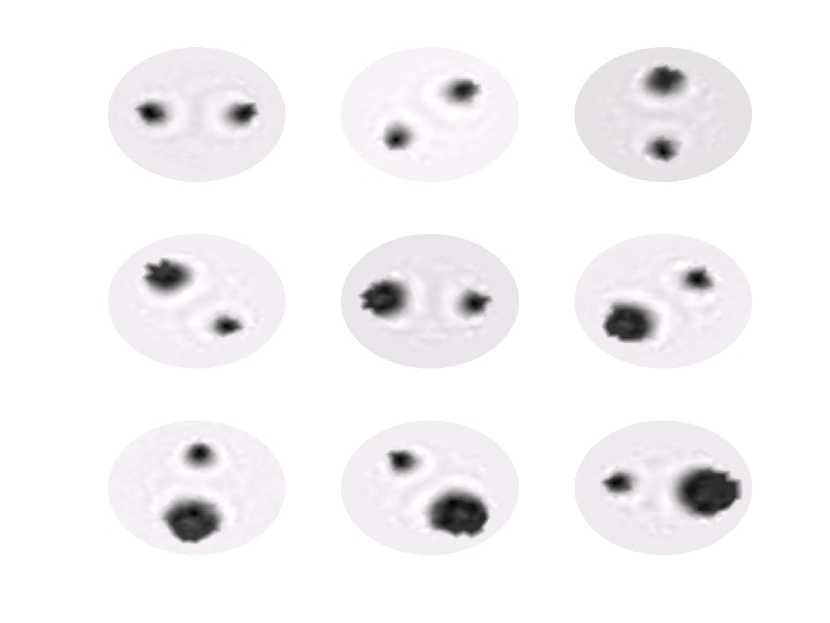
Figure 1: Reconstruction results for linearized data without noise.

For the second example we used the full nonlinear data $y=\Lambda_{1+\gamma(.,t)}-\Lambda_{1}\sim F^{\prime}(1)\gamma,$ and added $1\%$ white noise to the data. But for the computation of the evolution we still used the linearized operator $F^{\prime}(1)$. The results are shown in Figure 2. Also in this case - even with a systematical error due to the linearization - we still get fairly good results.

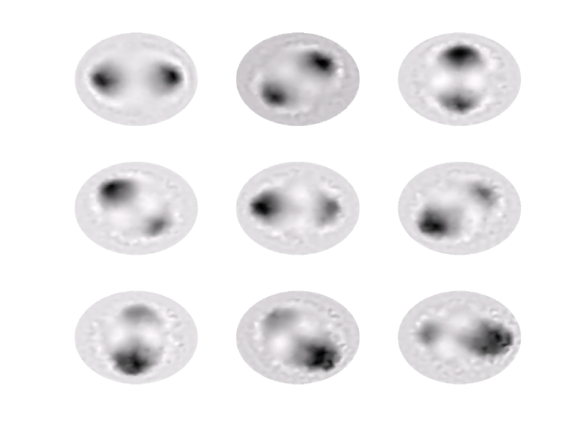
Figure 2: Reconstruction results for full nonlinear data with 1 % random noise.

5 Conclusions

Each method derived in this paper require, in a first step, the solution of an evolutionary equation (of Hamilton-Jacobi type). In a second step, the components of the solution vector $\{u_{k}\}$ are computed one at a time. This strategy reduces significantly both the size of the systems involved in the solution method, as well as storage requirements needed for the numerical implementation. These points turn out to become critical for long time measurement processes.

Some detailed considerations about complexity: Assume that all $F(t_{k})$ are discretized as $(n\times m)$ matrices. The main effort is the matrix multiplication for the update step for $Q_{k}$: In each step this requires $\mathcal{O}(n^{3}+n^{2}m)$ calculations. Hence the overall complexity is of the order $\mathcal{O}(n_{T}(n^{3}+n^{2}m))$ operations. If the discrete version is used, then in each step a matrix-inversion has to be performed, which is also of the order $\mathcal{O}(n^{3})$. which leads to the same complexity as above. In contrast, the method in [20] requires $\mathcal{O}((n+n_{T})^{3}+(n_{T}+m)nn_{T})$. Although this is only of cubic order in comparison to a quartic order complexity for the dynamic programming approach, it is cubic in $n_{T}$. Hence if $n_{T}$ is large, the method proposed in this paper (which is linear in $n_{T}$) will be more effective than the method in [20].

References

- [1] H. Ammari, G. Bao, J.L. Fleming, An inverse source problem for Maxwell’s equations in magnetoencephalography, SIAM J. Appl. Math. 62:1369–1382, 2002.
- [2] R. Bellman. An introduction to the theory of dynamic programming. The Rand Corporation, Santa Monica, California, 1953.
- [3] R. Bellman. Dynamic programming. Princeton University Press, Princeton, N.J., 1957.
- [4] R. Bellman, S.E. Dreyfus, E. Stuart. Applied dynamic programming. Princeton University Press, Princeton, N.J., 1962.
- [5] R. Bellman, R. Kalaba. Dynamic programming and modern control theory. Academic Press, New York – London, 1965.
- [6] M. Cheney, D. Isaacson, J.C. Newell. Electrical impedance tomography. SIAM Rev. 41:85–101, 1999.
- [7] H.W. Engl, M. Hanke, A. Neubauer. Regularization of Inverse Problems. Kluwer Academic Publishers, Dordrecht, 1996.
- [8] H.W. Engl, K. Kunisch, A. Neubauer. Convergence rates for Tikhonov regularization of nonlinear ill-posed problems. Inverse Problems 5:523–540, 1989.
- [9] H.W. Engl, O. Scherzer. Convergence rates results for iterative methods for solving nonlinear ill-posed problems. in D. Colton et al eds., Surveys on solution methods for inverse problems, Springer, Vienna, 2000.
- [10] M. Hanke, A. Neubauer, O. Scherzer. A convergence analysis of the Landweber iteration for nonlinear ill-posed problems. Numer. Math. 72:21–37, 1995.
- [11] S. Kindermann, A. Leitão. On regularization methods for inverse problems of dynamic type. Numerical Functional Analysis and Optimization, 27:139–160, 2006.
- [12] S. Kindermann, A. Leitão. On regularization methods based on dynamic programming techniques. BIT Numerical Mathematics (2006), to appear
- [13] S. Kindermann, C. Navasca. Optimal control as a regularization method for ill-posed problems. J. Inv. Ill-Posed Problems, 14, Nr. 5:1–19, 2006.
- [14] A.B. Kurzhanskiĭ, I.F. Sivergina. The dynamic programming method in inverse estimation problems for distributed systems. Doklady Mathematics 53:161–166, 1998.
- [15] A.B. Kurzhanskiĭ, I.F. Sivergina. Dynamic programming in problems of the identification of systems with distributed parameters. J. Appl. Math. Mech. 62:831–842, 1999.
- [16] C. Leondes, ed. Computational methods in biophysics, biomaterials, biotechnology and medical systems. Algorithm development, mathematical analysis, and diagnostics. Vol. 1: Algorithm techniques. Kluwer, Boston, 2003.
- [17] V.A. Morozov. Regularization Methods for Ill–Posed Problems. CRC Press, Boca Raton, 1993.
- [18] A.J. Peiton, ed. Invited papers from the first world congress on industrial process tomography, Buxton, April 14–17, 1999. Inverse Problems 16:461–517, 2000.
- [19] U. Schmitt, A.K. Louis, F. Darvas, H. Buchner, M. Fuchs. Numerical aspects of spatio-temporal current density reconstruction from EEG-/MEG-Data. IEEE Trans. Med. Imaging 20:314–324, 2001.
- [20] U. Schmitt, A.K. Louis. Efficient algorithms for the regularization of dynamic inverse problems I: Theory. Inverse Problems 18:645–658, 2002.
- [21] U. Schmitt, A.K. Louis, C. Wolters, M. Vauhkonen. Efficient algorithms for the regularization of dynamic inverse problems II: Applications. Inverse Problems 18:659–676, 2002.
- [22] U. Tautenhahn. On the asymptotical regularization of nonlinear ill-posed problems. Inverse Problems 10:1405–1418, 1994.
- [23] A. Seppänen, M. Vauhkonen, P.J.Vauhkonen, E.Somersalo, J.P Kaipio. State estimation with fluid dynamical evolution models in process tomography—an application to impedance tomography. Inverse Problems 17:467–483, 2001.
- [24] M. Vauhkonen, P.A. Karjalainen. A Kalman filter approach to track fast impedance changes in electrical impedance tomography. IEEE Trans. Biomed. Eng. 45:486–493, 1989.
- [25] R.A. Williams, M.S. Beck. Process Tomography, Principles, Techniques and Applications. Butterworth-Heinemann, Oxford, 1995.