Modeling stellar abundance patterns resulting from the addition of earthlike planetary material

Abstract

We model the observed precision differential abundance patterns of three G-type dwarfs, assuming a mass of planetary or disk material was added to or subtracted from the atmosphere of the star. The two-parameter model is fit by linear regression. The stellar abundance patterns are corrected for Galactic chemical evolution (GCE). The differential abundances can be highly correlated with the elemental condensation temperature. We show how it is possible to match not only the slope, but the quantitative abundance differences, assuming a composition for the added material equal to that of the bulk earth. We also model the wide pair HIP 34407 and HIP 34426, where GCE corrections are assumed unnecessary. An appendix discusses issues of volatility and condensation temperature.

1 Introduction

The literature on precision differential abundances (PDAs) in stars is extensive. Surveys include sun-like stars in the solar neighborhood, binary systems, and Galactic clusters. Numerous references as well as a discussion of relevant mechanisms may be found in papers by Ramírez, et al. (2019) and Nagar, Spina, & Karakas (2020). A strong impetus for this work is the probability that the abundances have been influenced by exoplanetary systems and their evolution.

We calculate the resulting differential abundances ($[El/H]$) assuming a given amount of material with the composition of the bulk earth (Wang, Lineweaver & Ireland, 2018, henceforth, WN18) was added to the stellar convection zone of a dwarf G-type star. The mass of the convection zone is uncertain and variable, depending on the spectral type. Here, we assume a mass of $5\cdot 10^{31}$ gm for the stellar convection zone (SCZ). This is 0.025 $M_{\odot}$ (cf. Pinsonneault, et al, 2001; Chambers, 2010). For other SCZ masses, the parameters must be adjusted accordingly. In general, the sunlike star will not have exactly the solar composition. This contingency is roughly taken into account in our model.

2 The model

Let $M_{SCZ}$ be the mass of the stellar convection zone. We use a bulk earth mass of $M_{BE}=6\cdot 10^{27}$ gm, with the composition from WN18. Our model assumes that as a result of the addition of $q$ earth masses of material, the stellar abundance of all elements will be increased by a factor of

$$\frac{q\cdot M_{BE}+p\cdot M_{SCZ}}{M_{SCZ}}=p+q\frac{M_{BE}}{M_{SCZ}}.$$ (1)

Note that the ratio of the masses, BE and SCZ, is the same as the ratio of the number of atoms in the BE and the SCZ.

The parameter $p$ allows for the possibility that the star may have abundances that differ slightly from those of the sun. If $p<1$, the star will be slightly metal poor, and conversely, if $p>1$, it will be slightly metal rich. Generally, we expect that $p$ will be close to unity. We assume the abundances vary in lockstep, and neglect small changes in the atmospheric structure resulting from the added material.

Using bracket notation, where $[X]=\log(X_{star})-\log(X_{sun})=\log(X_{star}/X_{sun})$,

$$[El/H]=\log\left(p+q\frac{M_{BE}}{M_{SCZ}}\right).$$ (2)

Rewriting Eq. 2 yields

$$p+q\frac{M_{BE}}{M_{SCZ}}=10^{[El/H]}.$$ (3)

We may obtain $p$ and $q$ by linear regression, as there is one equation for every differential elemental abundance. The regression fit includes the results of an $F$-test in which the $F$ statistic (the ratio of the varance for a one parameter fit to the variance for a two parameter fit) is calculated and used to establish a “significance” based on the Snedecor $F$ distribution. In this formalism, larger values of the $F$ statistic yield smaller significance measures; outcomes with significances substantially less than 0.01 demonstrate the superiority of the linear (two parameter) fit over that of flat line (one parameter or “mean”) fit. Values for $p$, $q$, $F$, and the significance are included in the discussions of the examples below.

3 Examples

Adibekyan, et al. (2014) pointed out that, in addition to correlations of differential abundances of solar-like stars with condensation temperature, $T_{\rm c}$, the PDAs also correlated with the stars’ ages and/or locations in the disk. These connections are readily seen as a consequence of Galactic chemical evolution (GCE), whose overall effect is to convert mostly light, volatile elements like carbon, nitrogen, and oxygen into heavier, refractory elements like iron, zirconium, and barium. Thus, stars younger than the sun are expected to be depleted in volatiles like C, N, and O but enhanced in refractories, such as Fe, Zr, and Ba, and heavier elements. This leads to a positive correlation of their differential abundances with condensation temperature. Note that most of the observable heavy elements have high $T_{\rm c}$. There are, of course, exceptions to this rough trend. Some heavy elements, such lead and mercury, are volatile, and the heavier noble gasses are ultra volatile. However abundance determinations for these elements are not usually available for G dwarfs.

It is necessary to subtract the effects of GCE prior to examining the differential abundances for possible effects of addition or subtraction of planetary material. This was done by Cowley, Bord & Yüce (2020a) in their study of $T_{\rm c}$ correlations among the 79 stars of Bedell, et al. (2018, henceforth, BD18) which included the first three examples below. BD18 give precision differential abundances for the following 30 elements: C, O, Na, Mg, Al, Si, S, Ca, Sc, Ti, V, Cr, Mn, Fe, Co, Ni, Cu, Zn, Sr, Y, Zr, Ba, La, Ce, Pr, Nd, Sm, Eu, Gd, and Dy.

In addition to GCE, the fascinating results of Meléndez, et al. (2014) for 18 Sco show that the abundances of neutron-addition (nA) elements (Sr-Dy in BD18) may be affected by local nucleosynthetic events unrelated to general GCE. In the current article we have not, therefore, included the nA elements in the fits of $[El/H]$ to $T_{\rm c}$ for HD 196390, HD 42618, and HD 140583.

3.1 Data sources

The calculations presented below require use of literature sources for condensation temperature, the composition of the bulk earth, and the composition of the convection zone. We have made numerous calculations based on different combinations of data sources, with the conclusion that for our purposes, differences in numerical values in the data sources are not significant.

In the current article, we report calculations from models based on two sets of data sources:

• Set I: Solar photospheric abundances from Amarsi, et al. (2018, 2019, 2020); Asplund, Grevesse & Sauval (2009), Lind, et al. (2017); Bergemann, et al. (2017); Carlos, et at. (2019); Grevesse, Scott & Asplund (2015), Norlander & Lind (2017); Osorio, et al. (2019); Riggiani, Amarsi & Lind (2019), Scott, Grevesse & Asplund (2015); Young (2018), condensation temperatures from Wood, et al. (2019), and bulk earth composition from Wang, Lineweaver & Ireland (2018).

• Set II: Solar abundances from Lodders (2020, see Table 6, Col 5). These abundances made partial use of CI determinations, as explained in the work cited. Condensation temperatures were from Lodders (2003), and bulk earth composition from McDonough & Arvelo, Jr. (2008).

We emphasize that for our purposes, which involve only the elements between carbon and zinc, the choice of data sources is not critical. As an illustration, we show in Tab. 1 that the derived model parameters of Eq. 3, $p$ and $q$, in data Sets I and II agree well.

Table 1: Model parameters from 2 data sets

Set	Star(s)	p	q	F	sig
Set I	HD 196390	1.07	5.0	54.0	1.4 E-07
Set II		1.09	5.4	38.8	1.2 E-06
Set I	HD 42618	0.81	-1.4	6.3	1.0E-02
Set II		0.80	-1.6	6.3	1.0E-02
Set I	HD 140538	0.97	4.6	19.1	7.5 E-05
Set II		1.00	4.4	8.3	3.7E-03
Set I	HIP34407/34426	1.28	8.2	19.7	2.9E-05
Set II		1.31	6.6	14.9	1.5E-04

3.2 HD 196390 (HIP 101905)

In Cowley, Bord & Yüce (2020a), six stars had differential abundances with significant ($<6.0\cdot 10^{-5}$) $T_{\rm c}$ correlations; the tightest correlation was for HD 196390.

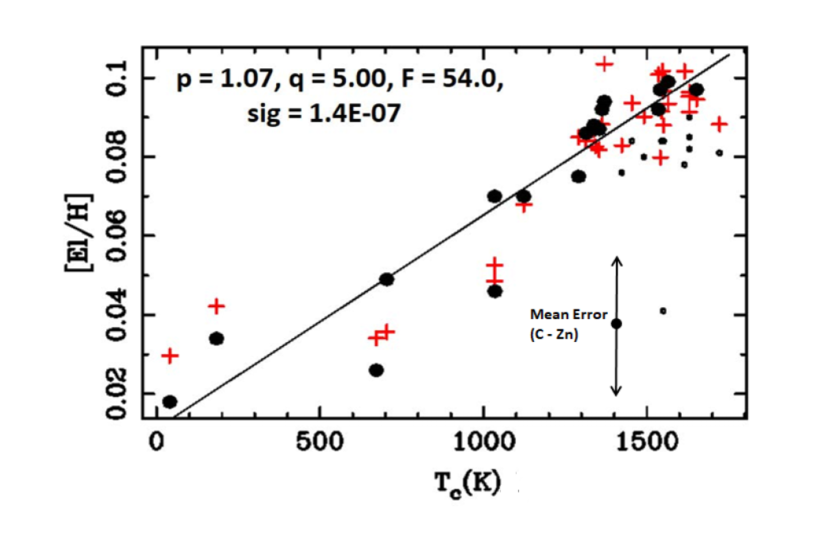
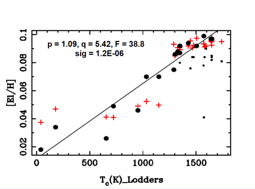
Figure 1: Left: Model predictions (red crosses) and observed differential stellar abundances (large black points) for HD 196390 vs. condensation temperature, $T_{\rm c}$, after GCE corrections. The parameters are from Set I of Tab. 1. The predicted abundances are from a slightly metal-rich model ($p=1.07$). The parameter $q=5.0$ implies that five earth masses were ingested. See text for further explanation of the symbols.
Right: Model predictions and observed differential stellar abundances for HD 196390 based on the parameters of Set II of Tab. 1. Symbols have the same meaning as at left. The two plots are closely similar. The predicted point (red plus sign at $T_{c}$ = 1158K) some 0.02 dex below the mean relation indicated by the solid black line is for Mn.

Model fits are shown in Fig. 1 based on data Sets I and II of Tab. 1. The straight line is an unweighted least squares fit to $[El/H]$ vs. $T_{\rm c}$ for carbon through zinc. The linear regression solution yielding $p$ and $q$ is also for these elements. Diffferences between observations and models, for both Sets I and II, are typically within the total uncertainties of the abundance measures, including the observational and analysis errors, plus those associated with the GCE correction parameters from BD18. These errors are indicated on the left plot. The small black dots designate the nA elements which were excluded from the modeling trials and the regression fits.

3.3 HD 42618 (HIP 29432)

Among the stars of BD18 noted by Cowley, Bord & Yüce (2020a), HD 42618 was unusual because of its negative slope, and because it has a known planet containing some 14.4 earth masses. The formal probability that an unweighted linear fit of $[El/H]$ with $T_{\rm c}$ occurs by chance was $2.1\cdot 10^{-5}$, but the two-parameter linear regression fit is only of marginal significance. Snedecor’s F-parameter is 6.3, leading to a significance level 0.010 (see Fig. 2, left). Data Sets I and II yield $p<1$ for this star, indicating that HD 42618 is slightly metal poor with respect to the sun. The negative values of $q$ suggest a deficit of earthlike material relative to the sun.

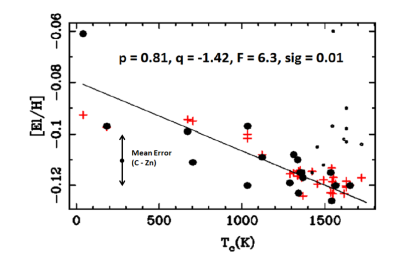
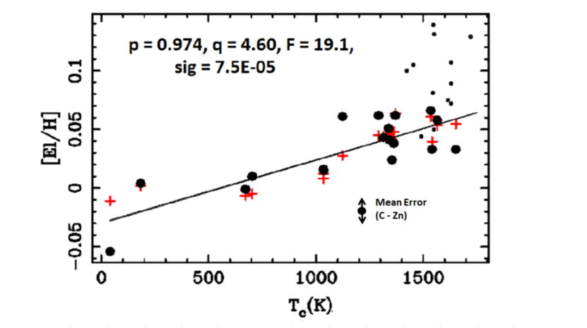
Figure 2: Left: Model predictions and observed differential stellar abundances for HD 42618 vs. condensation temperature after GCE corrections. The model abundances are slightly metal poor. The negative $q$-parameter implies that refractory mass is missing from HD 42618 relative to the sun.
Right: Model predictions and observed differential abundances for HD 140538 vs. condensation temperature after GCE corrections. The model abundances are close to solar, with $\approx 4.5$ earth masses of added material needed to optimize the fit to the observed PDAs.
Both plots use data and results from Set I.

3.4 HD 140538 (HIP 77052)

HD 140538 ($\psi$ Ser, Fig. 2, Right) is among the stars of Cowley, Bord & Yüce (2020a) which have a significant $[El/H]$ vs. $T_{\rm c}$ plot. Although classified as G2.5 V, it is not considered a solar twin possibly because it is thought to be in a triple system, with two dwarf M companions (Mahdi, et al., 2016). The $p$-parameters for both Sets I and II are near unity, indicating solar abundances for the 4 to 5 earth masses ($q$ parameter) added to HD 140538.

3.5 The wide double, HIP 34407 and HIP 34426

In the case of the binary pair, HIP 34407/HIP 34426, abundances are from Ramírez, et al. (2019) for 21 elements: Li, O, Na, Mg, Al, Si, S, K, Ca, Sc, Ti, V, Cr, Mn, Fe, Co, Ni, Cu, Zn, Y, and Ba. No GCE corrections were applied in this case, as we assume the stars are coevil. Moreover, if abundances for the two nA elements were perturbed by some isolated nucleosynthetic event, we assume both stars were equally influenced; thus, we include the nA elements Y and Ba in the model fit, based on data Set I.

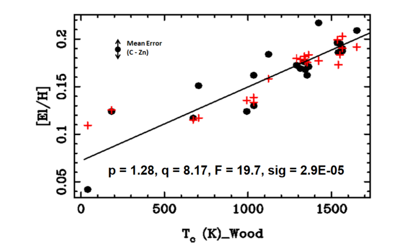
Figure 3: Model predictions and observed differential stellar abundances for HIP34407/HIP34426, where $[El/H]$ is $\log(El/H)_{\rm HIP34407}-\log(El/H)_{\rm HIP34426}$. Symbols have the same meaning as in Fig. 1. The model is based on data and results of Set I.

The comoving, closely similar G-stars, HIP 34407 and HIP 34426, were part of a larger work by Nagar, Spina, & Karakas (2020), who suggested the differential abundance pattern could result from the engulfment of a gas giant. The differential abundances are fit by addition of some 7 earth masses of material, the largest of the modeled stellar masses of this work. This is much lower than the total mass of a Jupiter-sized gas giant, but not so different from estimates of the core mass of heavy elements in Jupiter itself derived from models based on 1995 Galileo probe data (14 - 18 $M_{E}$, Militzer, et al. (2008)) and more recent results from the Juno mission (7 - 25 $M_{E}$, Wahl, et al. (2017)). We assume that the more volatile elements forming the bulk of the mass of captured gas giants would be lost during the engulfment process and not incorporated into the SCZ.

The lithium abundance in both stars is much higher than one would expect from their ages, which are greater than 6.5 Gyr for all plausible models according to Ramírez, et al. (2019), who give $\log(Li/H)+12=2.37$ for HIP 34407 and 2.31 for HIP 34426. Figs. 2-5 of Carlos, et at. (2019) show that only the youngest stars in the 79-star BD18 sample have comparable values with $\log(Li/H)+12\approx 2.3$. Ramírez, et al. (2019) discuss lithium abundances in both stars, but find no likely scenario to account for either the high individual abundances or the small abundance difference between the two stars. They compute $\Delta[Li/H]=\log(Li/H)_{\rm HIP34426}-\log(Li/H)_{\rm HIP34407}=-0.05$; this element is clearly above the trend for neighboring elements with similar condensation temperatures in their Fig. 4. In our Fig. 3, in which the roles of the two stars are reversed and $[El/H]$ is $\log(El/H)_{\rm HIP34407}-\log(El/H)_{\rm HIP34426}$, lithium would again be an obvious outlier in a plot with $[Li/H]=0.62$ at $T_{\rm c}=1148$K. Li is not included in the current model fit or plot.

4 Summary

In this paper, we have shown that some G-type stellar PDAs can be meaningfully interpreted by assuming that earth-like material was ingested by or missing from the modeled stars, perhaps through planetary formation processes. Four examples are presented in the form of plots of PDAs vs. $T_{\rm c}$, three with positive slopes and one with a negative slope. The derived model parameters confirm that the mean composition of the SCZs of these stars is essentially solar ($p_{avg}=1.03\pm 0.20$) as expected, but show a range of mass adjustments from -1.4 to +8.2 bulk earths. Predicted model abundances typically replicate the observed PDA distributions to within the observational errors which have mean values for the elements C through Zn ranging from 0.011 to 0.023 dex, including uncertainties associated with the parameters used to effect GCE corrections. We have tested our approach using two different sets of source data for the condensation temperatures, and the compositions for the bulk earth material and the initial stellar convection zone and find that, for the 30 elements included in our models, the results from the two sets are in good agreement.

While linear fits like those shown in our Figures 1 - 3 are adequate to describe the current results of PDA investigations which have generally been limited to 30 or so well-studied elements, such models would not properly describe $T_{\rm c}$ trends if precison abundance data for the full range of naturally occuring elements in the periodic table were available (cf. the Appendix). We argue that if the full range of abundances were available, the slope in the low-$T_{\rm c}$, volatile region should be essentially zero, while in the high-$T_{\rm c}$, refractory regime, the slope should also approach zero, although with much greater scatter.

Appendix A Condensation temperatures–accuracy and relevance

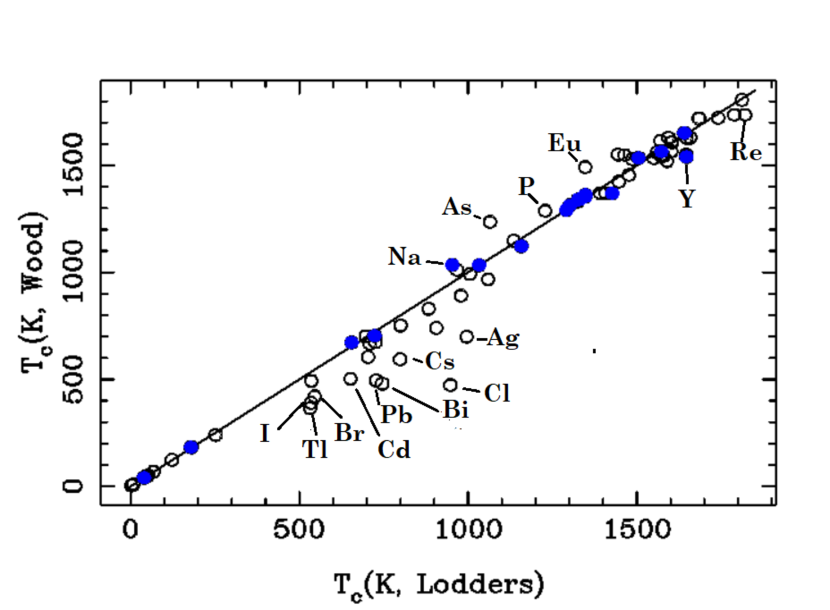
Figure 4: Condensation temperatures from Wood, et al. (2019) vs. those from Lodders (2003). The highlighted points are for the 18 elements used for the present models. Of those elements, sodium falls slightly above the 50-50 line, while yttrium falls slightly below. The latter element was used only in the model for HIP 34407/34426. Both deviations are small relative to the uncertainties of the overall model calculations presented in Sec. 3.

The relevance of condensation temperatures to cosmic solids was established by Wasson & Chou (1974). The 50% condensation temperatures of Lodders (2003), and the more recent values by Wood, et al. (2019), are in quite good agreement, apart from a few elements, viz. Cl, Pb, As, and Bi none of which are included in our modeling calculations (see Fig. 4). The assumptions underlying the determinations are more relevant. Both calculations begin with a gas of solar composition at a pressure of $10^{-4}$ bar, and assume strict chemical equilibrium–gas-solid reactions are allowed. A detailed discussion of equilibrium calculations and the geochemical classification of elements is given by Fegley & Schaefer (2010).

Barshay & Lewis (1976) discuss an alternate approach. “At the opposite extreme from the equilibrium model is the disequilibrium condensation model, which prohibits reactions between gas and already condensed phases, or between two or more condensed phases.” Details of their calculations, available in graphic form (see their Figs. 4 and 5), show qualitatively similar results. These figures also show that changes in the gas pressure from $10^{-2}$ to $10^{-6}$ bar do not significantly change the order of condensation. A useful recent discussion is by Li, et al. (2020) who give 2% condensation temperatures, also for a solar mix and a pressure of $10^{-4}$ bar, based on the GRAINS code of Petaev (2009). In all these calculations, volatile elements remain volatile and refractories refractory.

Table 2: Bulk earth: representative element abundance estimates

Element	Mc03	Mc08	WN18	% Error	50% $T_{\rm c}$(K)	VM
C	730	730	2 648	84	40	0.00469
N	25	57	31	87	123	0.000196
O	297 000	297 000	308 000	2.3	183	0.229
Zn	40	35	45.9	8.7	704	0.113
S	6 350	6 300	6 096	24	672	0.084
Cu	60	60	69	2.8	1034	0.420
Na	1 800	1 800	2 201	8.5	1035	0.345
Fe	320 000	319 000	312 000	0.3	1338	108
Mg	154 000	153 000	151 000	1.3	1343	1.00

Tab. 2 shows three estimates of the bulk earth abundance, for representative highly volatile, intermediate volatile, and refractory elements. Horizontal lines divide the three categories of volatility. Abundances are in parts per million by mass, from McDonough (2003, Mc03), McDonough & Arvelo, Jr. (2008, Mc08), and WN18. The fifth column gives WN18’s estimate of their errors in per cent. The condensation temperatures are from Wood, et al. (2019). The final column is a measure of the element’s volatility (VM). It gives the ratio:

$$VM=\left[\frac{\rm mass\ of\ element\ in\ earth}{\rm mass\ of\ magnesium\ in\ earth}\right]\div\left[\frac{\rm mass\ of\ element\ in\ sun}{\rm mass\ of\ magnesium\ in\ sun}\right]$$ (A1)

Tab. 2 illustrates the persistance of the property of volatility for different choices of earth models. Note that oxygen has an abundance that would put it with the involatiles, in spite of its low $T_{\rm c}$. This, of course, is because of the high reactivity of oxygen, so that it combines to form the ubiquitous silicates.

We conclude that statistically significant fits of $[El/H]$ data as a function of 50% $T_{\rm c}$, whether strictly linear, piece-wise linear, or logarithmic (cf. Wang, Lineweaver & Ireland, 2019), are robust indicators of the condensation of cosmic material, earthlike planets, or meteorites. The slopes of the relevant relations may be positive, zero or negative.

A.1 Insights from the full abundance table

In Fig. 5 (Left), we plot the $change$ in abundance values for the 30 elements studied in BD18 for an addition of two earth masses to a solar convection zone. Many stellar studies consider even fewer elements, and include only one or a few neutron-addition elements (e.g. Liu, et al., 2020). It is difficult to justify a more elaborate fit than a linear one, because of the scatter and sparseness of points especially at low $T_{\rm c}$. Workers typically attempt to fit the points with a straight line or line segments (cf. Liu, et al., 2020; Nissen, et al., 2020).

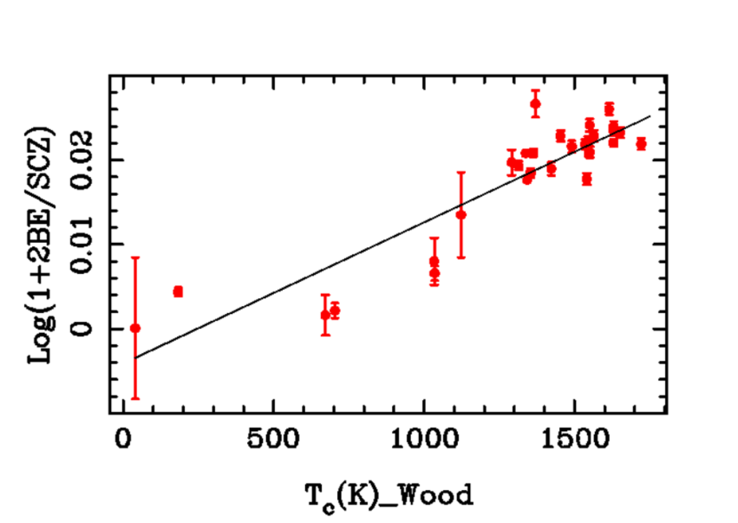
Figure 5: Left: Model calculations for the change in abundances associated with the ingestion of 2 bulk earths from WN18 for the 30 elements of the BD18 study. The error bars are from WN18; the largest is for carbon (leftmost point), whose abundance uncertainty is some 83%. Errors for other elements scale proportionally; the vertical scale does not apply to the errors.
Right: Same as the left panel, except plotted for all species in WN18. Points for elements whose solar and/or bulk earth (WN18) abundances are uncertain by $\geq$ 0.08 dex are designated by small open circles. A point for lithium is not plotted. The line is a simple trial and error fit $\propto 10^{-8.88}\cdot T_{\rm c}^{+2.32}$

Fig. 5 (Right) shows all elements from WN18 apart from lithium, which would be a high outlier at $T_{\rm c}=1148$K. It shows a much more detailed picture than Fig. 5 (Left). Using the full data from the WN18, we can explore the hypothesis of planet (or interplanetary debris) addition in greater detail when more stellar data points become available.

Elements with $T_{\rm c}<\sim 500$K are generally depleted and the logarithm of $(1+BE/SCZ)$ is essentially zero. The slope at low $T_{\rm c}$ would become appreciable only when some 20 bulk earth masses or more are added. If the peculiar abundance revealed by PDAs is due to the ingestion of only one or a few earth-like masses, the slope at small $T_{\rm c}$ should be close to zero.

Oxygen with $T_{\rm c}=40$K stands out above the trend for nearby elements in Fig. 5 (cf. Tab. 2) because much of it is incorporated in refractory silicate minerals. That explanation is not relevant for Pb ($T_{\rm c}=727,495$K), Ag ($T_{\rm c}=996,699$K), Au ($T_{\rm c}=1060,967$K), and Mn ($T_{\rm c}=1158,1123$K) (The first value is from Lodders (2003), the second from Wood, et al. (2019).) These points follow the overall trend as high outliers.

The plot for elements with $T_{\rm c}>\sim 1300$K shows a wide scatter but little evidence of a meaningful trend with $T_{\rm c}$. Some insight may be gained from plots similar to Fig. 5 (Right), but with compositions taken from meteorites (See Cowley, Bord, and Yüce, AAS237, iPoster 548.11, 2021). A recent discussion of these questions is given by Fegley, Lodders & Jacobson (2020), who show that much of the scatter at high $T_{\rm c}$ arises because of systematic abundance differences between refractory lithophile and siderophile elements (see their Figs. 3-5).

References

- Adibekyan, et al. (2014) Adibekyan, V. Zh., González Hernández, J. I., Delgado Mena, E., et al. 2014, A&A, 564, L15
- Amarsi & Asplund (2017) Amarsi, A. M. & Asplund, M. 2017, MNRAS, 464, 264
- Amarsi, et al. (2018) Amarsi, A. M., Barklem, P. S., Asplund, M., et al. 2018, 616, 89
- Amarsi, et al. (2019) Amarsi, A. M., Barkelm, P. W., Collet, R., et al. 2019, A&A, 624, 111
- Amarsi, et al. (2020) Amarsi, A. M., Grevesse, N., Grumer, J., et al. 2020, A&A, 636, 120
- Asplund, Grevesse & Sauval (2009) Asplund, M., Grevesse, N. & Sauval, J. 2009, ARAA, 47, 481
- Barshay & Lewis (1976) Barshay, S. S. & Lewis, J. S. 1976, Ann. Rev. Astron. Ap., 14, 81
- Bedell, et al. (2018) Bedell, M., Bean, J. L., Meléndez, J., et al. 2018, ApJ, 865, 68 (BD18)
- Bergemann, et al. (2017) Bergemann, M., Collet, R., Amarsi, A. M., et al. 2017, ApJ, 847, 15
- Bergemann, et al. (2019) Bergemann, M., Gallagher, A. J., Eitner, P., et al. 2019, A&A, 631, 80
- Carlos, et at. (2019) Carlos, M., Meléndez, J., Spina, L., et al. 2019, MNRAS, 485, 4052
- Chambers (2010) Chambers, J. E., 2010, ApJ, 724, 92
- Cowley, Bord & Yüce (2020a) Cowley, C. R., Bord, D. J. & Yüce, K. 2020a, RNAAS, 4, 31
- Fegley & Schaefer (2010) Fegley, B., Jr. & Schaefer, L. 2010, in Principles and Perspectives in Cosmochemistry, Astrophys. Sp. Sci. Proceedings (ed. A. Goswami & B. E. Reddy, Berlin: Springer-Verlag)
- Fegley, Lodders & Jacobson (2020) Fegley, B., Jr., Lodders, K. & Jacobson, N. S. 2020, Geochemistry, 80, 125594
- Grevesse, Scott & Asplund (2015) Grevesse, N., Scott, P. & Asplund, M. 2015, A&A, 573, 27G
- Li, et al. (2020) Li, M., Huang, S., Petaev, M. I. et al. 2020, MNRAS, 495, 2543
- Liu, et al. (2020) Liu, F., Yong, D., Asplund, M. et al. 2020, MNRAS, 495, 3961
- Lawler, et al. (2019) Lawler, J. E., Hala, Sneden, C., et al. 2019, ApJS, 241, 21
- Lind, et al. (2017) Lind, K., Amarsi, A. M., Asplund, M., et al. 2017, MNRAS 468, 4311
- Lodders (2003) Lodders, K. 2003, ApJ, 591, 1220
- Lodders (2020) Lodders, K. 2020, in The Oxford Research Encyclopedia of Planetary Science, ed. Peter Read (Oxford: Oxford University Press)
- Mahdi, et al. (2016) Mahdi, D., Soubiran, C., Blanco-Cuaresma, S. & Chemin, L. 2016, A&A, 587, 131
- McDonough (2003) McDonough, W. F. 2003, Treatise on Geochem., Vol. 2., 547
- McDonough & Arvelo, Jr. (2008) McDonough, W. F. & Arevalo, Jr., R. 2008, J. Phys. Conf. Ser., 136, 022006
- Meléndez, et al. (2014) Meléndez, J., Ramírez, I., Karakas, A., et al. 2014, ApJ, 791, 14
- Militzer, et al. (2008) Militzer, B., Hubbard, W. B., Vorbeger, J., et al. 2008, ApJ, 688, L45
- Nagar, Spina, & Karakas (2020) Nagar, T., Spina, L. & Karakas, A. 2020, ApJ, 888, L9
- Nissen, et al. (2020) Nissen, P. E., Christensen-Dalsgaard, J., Mosumgaard, J. R. et al. 2020, A&A, 640, A81
- Norlander & Lind (2017) Norlander, T. & Lind, K. 2017, A&A, 607, 75
- Osorio, et al. (2019) Osorio, Y., Lind, K., Barklem, P. S., et al. 2019, A&A, 623, 1030
- Petaev (2009) Petaev, M. I. 2009, CALPHAD, 33, 317
- Pinsonneault, et al (2001) Pinsonneault, M. H., DePoy, D. L. & Coffee, M. 2001, ApJ, 556, L59
- Ramírez, et al. (2019) Ramírez, I., Khanal, S., Lichon, S. J., et al. 2019, MNRAS, 490, 2448
- Riggiani, Amarsi & Lind (2019) Riggiani, H., Amarsi, A. M. & Lind, K. 2019, A&A, 627, 177
- Scott, Grevesse & Asplund (2015) Scott, P., Grevesse, N. & Asplund, M. 2015, A&A, 573, A27
- Wahl, et al. (2017) Wahl, S. M., Hubbard, W. B., Militzer, B., et al. 2017. Geophys. Res. Letters, 44, 4649
- Wang, Lineweaver & Ireland (2018) Wang, H. S., Lineweaver, C. H. & Ireland, T. R. 2018, Icarus, 299, 460 (WN18)
- Wang, Lineweaver & Ireland (2019) Wang, H. S., Lineweaver, C. H. & Ireland, T. R. 2019, Icarus, 328, 287
- Wasson & Chou (1974) Wasson, J. T. & Chou, C.-L. 1974, Meteoritics, 9, 69
- Wenger, et al. (2000) Wenger, M., Ochsenbein, F., Egret, D., et al. 2000, A&AS, 143, 9
- Wood, et al. (2019) Wood, B. J., Smythe, D. J. & Harrison, T. 2019, AmMin, 104, 844
- Young (2018) Young, P. R. 2018, ApJ, 855, 15