Reinforcement Learning with Soft Temporal Logic Constraints Using Limit-Deterministic Generalized Büchi Automaton

Abstract

This paper studies the control synthesis of motion planning subject to uncertainties. The uncertainties are considered in robot motions and environment properties, giving rise to the probabilistic labeled Markov decision process (PL-MDP). A Model-Free Reinforcement The learning (RL) method is developed to generate a finite-memory control policy to satisfy high-level tasks expressed in linear temporal logic (LTL) formulas. Due to uncertainties and potentially conflicting tasks, this work focuses on infeasible LTL specifications, where a relaxed LTL constraint is developed to allow the agent to revise its motion plan and take violations of original tasks into account for partial satisfaction. And a novel automaton is developed to improve the density of accepting rewards and enable deterministic policies. We proposed an RL framework with rigorous analysis that is guaranteed to achieve multiple objectives in decreasing order: 1) satisfying the acceptance condition of relaxed product MDP and 2) reducing the violation cost over long-term behaviors. We provide simulation and experimental results to validate the performance.

I INTRODUCTION

Formal logic is capable of describing complex high-level tasks beyond traditional go-to-goal navigation for robotic systems. As a formal language, linear temporal logic (LTL) has been increasingly used in the motion planning of robotic systems [1, 2, 3]. Since robotic systems are often subject to a variety of uncertainties arising from the stochastic behaviors of the motion (e.g., an agent may not exactly follow the control inputs due to potential sensing noise or actuation failures) and uncertain environment properties (e.g., there exist mobile obstacles or time-varying areas of interest), Markov decision processes (MDPs) are often used to model the probabilistic motion of robotic systems [4]. Based on probabilistic model checking, control synthesis of MDP with LTL motion specifications has been widely investigated (cf. [5, 6, 7, 8, 9, 10]). In particular, the topic of partial satisfaction of high-level tasks in deterministic and stochastic systems is investigated in [11, 12, 9, 13]. Yet, new challenges arise when considering motion and environment uncertainties. Hence, learning to find a satisfying policy is paramount for the robot to operate in the presence of motion and environment uncertainties.

Reinforcement learning (RL) is a sequential decision-making process in which an agent continuously interacts with and learns from the environment [14]. Model-based RL has been employed for motion planning with LTL specifications when full knowledge of MDP is available [15]. The work of [16] extends model-based RL to temporal logic constrained control of stochastic systems with unknown parameters by model approximation. In [17] and [18], transition probabilities are learned to facilitate the satisfaction of LTL specifications. However, these aforementioned works have to reply on the accuracy of transition probabilities for learning. On the other hand, model-free RL approaches with LTL-based rewards generate desired policies by directly optimizing the Q-values [19, 20, 21, 22]. However, these works are based on a key assumption that at least an accepting maximum end component (AMEC) exists in a standard product MDP [1], which may not be true in practice. For instance, some areas of interest to be visited can be probabilistically prohibitive to the agent in practice (e.g., potentially surrounded by water due to heavy rain that the ground robot cannot traverse), resulting in part of the user-specified tasks cannot be achieved and AMECs do not exist in the product MDP. Although minimal revision of motion plans in a potentially conflicting environment has been investigated in the works of [23, 24, 25, 26], only deterministic transition systems are considered, and it is not yet clear how to address the above-mentioned issues in stochastic systems i.e., MDP.

Related Works: Compared with most RL-based approaches [17, 21, 22, 27], the reward functions are generally designed to enforce the convergence to AMECs so that the acceptance condition can be satisfied. However, these approaches are not applicable in this work since AMECs may not even exist due to environmental uncertainties. Thus, the probability of satisfying the pre-specified tasks may become zero. As an alternative solution, the work of [28] proposes a reduced variance deep Q-learning method to approximate optimal state-action values. In addition, our previous work [29] develops a relaxed product MDP, in which LTL formulas are converted into Deterministic Rabin Automaton (DRA) without assuming the existence of AMECs. However, the authors in [21] claim that it may fail to find desired policies by converting LTL into DRA. Even though our recent work [30] shows how to leverage planning algorithms to guide minimally-violating policies for infeasible LTL tasks. But multi-objective reinforcement learning without the assistance of planning is still under investigation.

In [31], the LDGBA is applied, and a synchronous frontier function for RL reward is designed to synthesize control policies that mostly fulfill the given task by maximizing the visits of the accepting sets in LDGBA. However, it cannot record the visited or non-visited accepting sets in each round. As an extension of [29], this work can handle the above issues by developing an E-LDGBA to record the non-visited accepting sets without adding extra computational complexity. The proposed relaxed product MDP and the designed utility function transforms the control synthesis problem into an expected utility optimization problem, in which a satisfactory policy is guaranteed to be found by leveraging RL to optimize the expected utility. Instead of DRA, LDGBA is used to reduce the size of the automaton. It is well known that the Rabin automaton, in the worst case, is doubly exponential in the size of the LTL formula, while LDGBA for many LTL formulas is an exponentially-sized automaton [32]. Moreover, the model-free RL-based approach is adopted and can synthesize optimal policies on-the-fly without explicitly memorizing structures of relaxed product MDP.

Contributions: Motivated by these challenges, this work considers the transition probabilities of interactions between the environment and the mobile robot to be unknown. We study learning-based motion planning subject to uncertainties, where control objectives are defined as high-level LTL formulas to express complex tasks. The contributions of this work are multi-fold. (i). From the aspect of automaton theory, we leverage an embedded limit deterministic generalized Büchi automaton (E-LDGBA) that has several accepting sets to maintain a dense reward and allows applying deterministic policies to achieve high-level objectives. (ii) Both motion and workspace uncertainties are considered to be unknown, leading to potentially conflicting tasks (i.e., the pre-specified LTL tasks cannot be fully satisfied). We design a relaxed product MDP from the PL-MDP and the novel automaton so that the RL agent can revise its motion plan without strictly following the desired LTL constraints. (iii) An expected return composed of violation rewards and accepting rewards is developed. The designed violation function quantifies the differences between the revised and the desired motion plans, while the accepting rewards enhance the satisfaction of the acceptance condition of the relaxed product MDP. (iv) Rigorous analysis is provided to show how to properly design parameters of accepting and violating rewards for multi-objective RL (MORL). Based on that, the RL agent can find policies that fulfill pre-specified tasks as much as possible.

II PRELIMINARIES

II-A Probabilistic Labeled MDP

Definition 1.

A probabilistic labeled MDP (PL-MDP) is a tuple $\mathcal{M}=(S,A,p_{S},(s_{0},l_{0}),\Pi,L,p_{L},\varLambda)$, where $S$ is a finite state space; $A$ is a finite action space; $p_{S}:S\times A\times S\shortrightarrow\left[0,1\right]$ is the transition probability function; $\Pi$ is a set of atomic propositions; and $L:S\shortrightarrow 2^{\Pi}$ is a labeling function. Let $\xi$ be an action function, which can be either deterministic such that $\xi:S\rightarrow A$ maps a state $s\in S$ to an action in $A(s)$, or randomized such that $\xi:S\times A\rightarrow\left[0,1\right]$ represents the probability of taking an action in $A(s)$ at $s$. The pair $(s_{0},l_{0})$ denotes an initial state $s_{0}\in S$ with an initial label $l_{0}\in L(s_{0})$. The function $p_{L}(s,l)$ denotes the probability of $l\in L(s)$ associated with $s\in S$ satisfying $\sum_{l\in L(s)}p_{L}(s,l)=1,\forall s\in S$. The transition probability $p_{S}$ captures the motion uncertainties of the agent while the labeling probability $p_{L}$ captures the environment uncertainties.

It is assumed that the agent can fully observe its current state and the associated labels. The PL-MDP can be regarded as an advanced MDP, and we can use the MDP to denote it in the following sections. The MDP $\mathcal{M}$ evolves by taking actions $\xi_{i}$ at each stage $i$, where $i\in\mathbb{N}_{0}$ with $\mathbb{N}$ being the set of natural numbers.

Definition 2.

The control policy $\boldsymbol{\mu}=\mu_{0}\mu_{1}\ldots$ is a sequence of decision rules, which yields a path $\boldsymbol{s}=s_{0}s_{1}s_{2}\ldots$ over $\mathcal{M}$ with $p_{S}(s_{i},a_{i},s_{i+1})>0$ for all $i$. $\boldsymbol{\mu}$ can be either deterministic such that $\boldsymbol{\mu}:S\rightarrow A$ or stochastic such that $\boldsymbol{\mu}:S\times A\rightarrow\left[0,1\right]$. The control policy $\boldsymbol{\mu}$ is memoryless if each $\mu_{i}$ only depends on its current state $s_{i}$. In contrast, $\boldsymbol{\mu}$ is called a finite-memory (i.e., history-dependent) policy if $\mu_{i}$ depends on its past states.

This work shows how to apply the deterministic and memoryless policy that has more stable decision-making performance. Let $\boldsymbol{\mu}(s)$ denote the probability distribution of actions at state $s$, and $\boldsymbol{\mu}(s,a)$ represents the probability of generating action $a$ at state $s$ using the policy $\boldsymbol{\mu}$. Let $\varLambda:S\shortrightarrow\mathbb{R}$ denote a reward function over $\mathcal{\mathcal{M}}$. Given a discount factor $\gamma\in(0,1)$, the expected return under policy $\xi$ starting from $s\in S$ can be defined as

$$U^{\xi}(s)=\mathbb{E}^{\xi}\left[\stackrel{{\scriptstyle[}}{{i}}=0]{\infty}{\sum}\gamma^{i}\varLambda(s_{i})\left|s_{0}=s\right.\right]$$ (1)

The optimal policy $\xi^{*}$ is a policy that maximizes the expected return for each state $s\in S$ as $\xi^{*}=\underset{\xi}{\arg\max}U^{\xi}(s).$

Definition 3.

Given a PL-MDP $\mathcal{M}$ under policy $\boldsymbol{\pi}$, a Markov chain $MC_{\mathcal{M}}^{\boldsymbol{\mu}}$ of the PL-MDP $\mathcal{M}$ induced by a policy $\boldsymbol{\mu}$ is a tuple $(S,A,p^{\boldsymbol{\mu}}_{S},(s_{0},l_{0}),L,p_{L})$ where $p^{\boldsymbol{\mu}}_{S}(s,s^{\prime})=p_{S}(s,a,s^{\prime})$ with $\boldsymbol{\mu}(s,a)>0$ for all $s,s^{\prime}\in S$.

A sub-MDP $\mathcal{M}{}_{(S^{\prime},A^{\prime})}$ of $\mathcal{M}$ is a pair $(S^{\prime},A^{\prime})$ where $S^{\prime}\subseteq S$ and $A^{\prime}$ is a finite action space of $S^{\prime}$ such that (i) $S^{\prime}\neq\emptyset$, and $A^{\prime}(s)\neq\emptyset,\forall s\in S^{\prime}$; (ii) $\left\{s^{\prime}\mid\forall s\in S^{\prime}\text{ and }\forall a\in A^{\prime}(x),p^{\mathcal{P}}(s,a,s^{\prime})>0\right\}\subseteq S^{\prime}$. An induced graph of $\mathcal{M}{}_{(S^{\prime},A^{\prime})}$ is denoted as $\mathcal{G}_{(S^{\prime},A^{\prime})}$ that is a directed graph, where if $p_{S}(s,a,s^{\prime})>0$ with $a\in A^{\prime}(s)$, for any $s,s^{\prime}\in S^{\prime}$, there exists an edge between $s$ and $s^{\prime}$ in $\mathcal{G}_{(S^{\prime},A^{\prime})}$. Note the evolution of a sub-MDP $\mathcal{M}{}_{(S^{\prime},A^{\prime})}$ is restricted by the action space $A^{\prime}$. A sub-MDP is a strongly connected component (SCC) if its induced graph is strongly connected such that for all pairs of nodes $s,s^{\prime}\in S^{\prime}$, there is a path from $s$ to $s^{\prime}$. A bottom strongly connected component (BSCC) is an SCC from which no state outside is reachable by applying the restricted action space. More details of the MDP treatments can be found in [1].

Definition 4.

[1] A sub-MDP $\mathcal{M}{}_{(S^{\prime},A^{\prime})}$ is an end component (EC) of $\mathcal{M}$ if it’s a BSCC. An EC $\mathcal{M}{}_{(S^{\prime},A^{\prime})}$ is called a maximal end component (MEC) if there is no other EC $\mathcal{M}{}_{(S^{\prime\prime},A^{\prime\prime})}$ such that $S^{\prime}\subseteq S^{\prime\prime}$ and $A^{\prime}(s)\subseteq A^{\prime\prime}(s)$, $\forall s\in S$.

II-B LTL and Limit-Deterministic Generalized Büchi Automaton

Linear temporal logic is a formal language to describe the high-level specifications of a system. An LTL formula is built on a set of atomic propositions, e.g., $a\in{AP}$, standard Boolean operators such as $\land$ (conjunction), $\lnot$ (negation), and temporal operators $\mathcal{U}$ (until), $\varbigcirc$ (next), $\diamondsuit$ (eventually), $\boxempty$ (always). The syntax of an LTL formula is defined inductively as

$$\phi:=\text{True}\mid a\mid\phi_{1}\land\phi_{2}\mid\lnot\phi\mid\phi\mid\phi_{1}\mathcal{U}\phi_{2}\>,$$

The semantics of an LTL formula are interpreted over words, which is an infinite sequence $\boldsymbol{o}=o_{0}o_{1}\ldots$ where $o_{i}\in 2^{{AP}}$ for all $i\geq 0$, and $2^{{AP}}$ represents the power set of ${AP}$, which are defined as:

$$\begin{array}[]{lcl}\boldsymbol{o}\models\text{true}\\ \boldsymbol{o}\models\alpha&\Leftrightarrow&\alpha\in L(\boldsymbol{o}[0])\\ \boldsymbol{o}\models\phi_{1}\land\phi_{2}&\Leftrightarrow&\boldsymbol{o}\models\phi_{1}\text{ and }\boldsymbol{o}\models\phi_{2}\\ \boldsymbol{o}\models\lnot\phi&\Leftrightarrow&\boldsymbol{o}\mid\neq\phi\\ \boldsymbol{o}\models\phi&\Leftrightarrow&\boldsymbol{o}[1:]\models\phi\\ \boldsymbol{o}\models\phi_{1}\mathcal{U}\phi_{2}&\Leftrightarrow&\exists t\text{ s.t. }\boldsymbol{o}[t:]\models\phi_{2},\forall t^{\prime}\in[0,t),\boldsymbol{o}[t^{\prime}:]\models\phi_{1}\\ \end{array}$$

Denote by $\boldsymbol{o}\models\varphi$ if the word $\boldsymbol{o}$ satisfies the LTL formula $\varphi$. More expressions can be achieved by combing temporal and Boolean operators. Detailed descriptions of the syntax and semantics of LTL can be found in [1]. Given an LTL formula that specifies the missions, the satisfaction of the LTL formula can be evaluated by an LDGBA [32].

Definition 5.

A GBA is a tuple $\mathcal{A}=(Q,\Sigma,\delta,q_{0},F)$, where $Q$ is a finite set of states, $\Sigma=2^{\Pi}$ is a finite alphabet; $\delta\colon Q\times\Sigma\shortrightarrow 2^{Q}$ is a transition function, $q_{0}\in Q$ is an initial state, and $F=\left\{F_{1},F_{2},\ldots,F_{f}\right\}$ is a set of acceptance conditions with $F_{i}\subseteq Q$, $\forall i\in\left\{1,\ldots f\right\}$.

Denote by $\boldsymbol{q}=q_{0}q_{1}\ldots$ a run of a GBA, where $q_{i}\in Q$, $i=0,1,\ldots$. The run $\boldsymbol{q}$ is accepted by the GBA, if it satisfies the generalized Büchi accepting sets, i.e., $\inf(\boldsymbol{q})\cap F_{i}\neq\emptyset$, $\forall i\in\left\{1,\ldots f\right\}$, where $\inf(\boldsymbol{q})$ denotes the set of states that is visited infinitely often.

Definition 6.

A GBA is a Limit-deterministic Generalized Büchi automaton (LDGBA) if $\delta\colon Q\times(\Sigma\cup\left\{\epsilon\right\})\shortrightarrow 2^{Q}$ is a transition function, and the states $Q$ can be partitioned into a deterministic set $Q_{D}$ and a non-deterministic set $Q_{N}$, i.e., $Q_{D}\cup Q_{N}=Q$ and $Q_{D}\cap Q_{N}=\emptyset$, where

• the state transitions in $Q_{D}$ are total and restricted within it, i.e., $\bigl{|}\delta(q,\alpha)\bigr{|}=1$ and $\delta(q,\alpha)\subseteq Q_{D}$ for every state $q\in Q_{D}$ and $\alpha\in\Sigma$,

• the $\epsilon$-transitions are only defined for state transitions from $Q_{N}$ to $Q_{D}$, and are not allowed in the deterministic set i.e., for any $q\in Q_{D}$, $\delta(q,\epsilon)=\emptyset,\forall\epsilon\in\left\{\epsilon\right\}$,

• the accepting states are only in the deterministic set, i.e., $F_{i}\subseteq Q_{D}$ for every $F_{i}\in F$.

In Def. 6, the $\epsilon$-transitions are only defined for state transitions from $Q_{N}$ to $Q_{D}$ that do not consume the input atomic proposition. Readers are referred to [33] for algorithms with free implementations to convert an LTL formula to an LDGBA,. Note that the state-based LDGBA is used in this work for demonstration purposes. Transition-based LDGBA can be constructed based on basic graph transformations. More discussions about state-based and transition-based LDGBA in HOA format can be found in Owl [34].

Remark 1.

Unlike the widely used deterministic Rabin Automaton (DRA), LDGBA has the Generalized Büchi Accepting condition that purely involves reachability problems. On the other hand, compared with Limit-Deterministic Büchi Automaton (LDBA) applied in [22, 21], LDGBA has more accepting sets shown in Fig.1 (a) to increase the density of rewards since the positive rewards are always assigned to the accepting states to enforce the acceptance condition.

III Problem Statement and Challenge

The task specification to be performed by the agent is described by an LTL formula $\phi$ over $\Pi$. Given $\phi$, $\mathcal{M},$ and $\boldsymbol{\xi}=\xi_{0}\xi_{1}\ldots$, the induced infinite path is denoted by $\boldsymbol{s}_{\infty}^{\boldsymbol{\xi}}=s_{0}\ldots s_{i}s_{i+1}\ldots$ that satisfies $s_{i+1}\in\left\{s\in S\bigl{|}p_{S}(s_{i},a_{i},s)>0\right\}$. Let $L(\boldsymbol{s}_{\infty}^{\boldsymbol{\xi}})=l_{0}l_{1}\ldots$ be the sequence of labels associated with $\boldsymbol{s}_{\infty}^{\boldsymbol{\xi}}$ such that $l_{i}\in L(s_{i})$ and $p_{L}(s_{i},l_{i})>0$. Denote by $L(\boldsymbol{s}_{\infty}^{\boldsymbol{\xi}})\models\phi$ if $\boldsymbol{s}_{\infty}^{\boldsymbol{\xi}}$ satisfies $\phi$. The satisfaction probability under $\boldsymbol{\mu}$ from an initial state $s_{0}$ can be computed as

$$\mathbb{\Pr}_{\mathcal{M}}^{\boldsymbol{\mu}}(\phi)=\mathbb{\Pr}_{\mathcal{M}}^{\boldsymbol{\mu}}(\boldsymbol{s}_{\infty}^{\boldsymbol{\mu}}\in\boldsymbol{S}_{\infty}^{\boldsymbol{\mu}}\left.\right|L(\boldsymbol{s}_{\infty}^{\boldsymbol{\mu}})\models\phi),$$ (2)

where $\boldsymbol{S}_{\infty}^{\boldsymbol{\mu}}$ is a set of all admissible paths under policy $\boldsymbol{\mu}$, and the computation of $\mathbb{\Pr}_{\mathcal{M}}^{\boldsymbol{\mu}}(\boldsymbol{s}_{\infty}^{\boldsymbol{\mu}})$ can be found in [1].

Definition 7.

Given a PL-MDP $\mathcal{M}$, an LTL task $\phi$ is fully feasible if and only if $\mathbb{\Pr}_{\mathcal{M}}^{\boldsymbol{\mu}}(\phi)>0$ s.t. there exists a path $\boldsymbol{s}_{\infty}^{\boldsymbol{\mu}}$ over the infinite horizons under the policy $\boldsymbol{\mu}$ satisfying $\phi$.

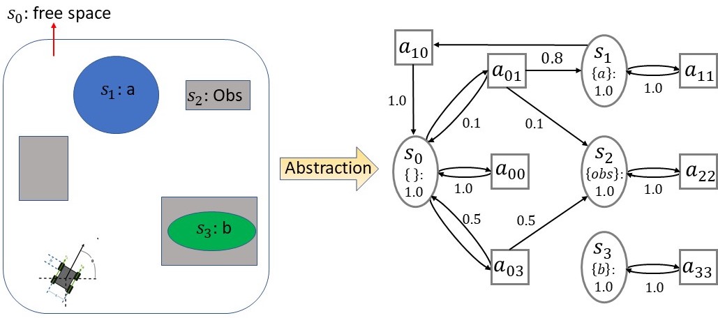
(a)

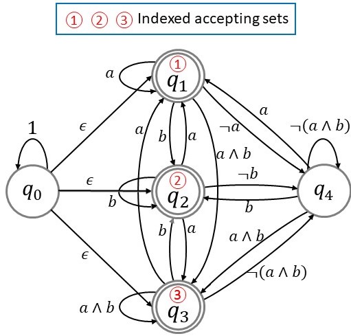
(b)

      

Figure 1: A running example of an infeasible LTL task with respect to the PL-MDP. (a) The abstraction process from a robotic system into a PL-MDP $\mathcal{M}$, where the region labeled with $b$ is surrounded by obstacles and can not be accessed. As a result, $\phi$ is infeasible in this case. (b) The LDGBA of an LTL formula $\phi=\oblong\lozenge\mathtt{a}\land\oblong\lozenge\mathtt{b}$.

Based on Def. 7, an infeasible case means there does not exist any policy $\mu$ to satisfy the task i.e., $\mathbb{\Pr}_{\mathcal{M}}^{\boldsymbol{\mu}}(\phi)=0$.

Example 1.

To illustrate an infeasible case, the environment, its abstracted PL-MDP, and the LDGBA of an LTL formula $\phi=\oblong\lozenge\mathtt{a}\land\oblong\lozenge\mathtt{b}$ are shown in Fig. 1 (a) and (b), respectively. Since obstacles surround region $s_{3}$, the given LTL task is infeasible in this case.

We define the expected discount violation cost of task satisfaction as follows, considering feasible and infeasible tasks.

Definition 8.

Given a PL-MDP $\mathcal{M}$ and an LTL task $\phi$, the discount expected violation under the policy $\boldsymbol{\mu}$ is defined as

$$J_{V}(\mathcal{M}^{\boldsymbol{\mu}},\phi)=\mathbb{E}_{\mathcal{M}}^{\boldsymbol{\mu}}\left[\stackrel{{\scriptstyle[}}{{i}}=0]{\infty}{\sum}\gamma^{i}c_{V}(s_{i},a_{i},s_{i+1},\phi)\right],$$ (3)

where $c_{V}(s,a,s^{\prime},\phi)$ is defined as the violation cost of a transition $(s,a,s^{\prime})$ with respect to $\phi$, and $a_{i}$ is the action generated based on the policy $\boldsymbol{\mu}(s_{i})$.

Most existing results (cf. [17, 21, 22]) assume the existence of at least one policy $\mu$ s.t. $\mathbb{\Pr}_{\mathcal{M}}^{\boldsymbol{\mu}}(\phi)>0$, which may not be true in practice if the task is only partially feasible. In addition, previous work [13] addresses the infeasible cases via an optimization approach that assumes the transitions probabilities of $\mathcal{M}$ are known. We remove this assumption and apply the RL approach to learn the desired policies in this work. We consider the following problem to account for challenges of both infeasible cases and unknown transitions.

Problem 1.

Given an LTL-specified task $\phi$ and a PL-MDP with unknown transition probabilities (i.e., motion uncertainties) and unknown probabilistic label functions (i.e., workspace uncertainties), the objective is to find a policy (1) $\mathbb{\Pr}_{\mathcal{M}}^{\boldsymbol{\mu}}(\phi)>0$ if it exists; (2) if $\forall\boldsymbol{\mu},\mathbb{\Pr}_{\mathcal{M}}^{\boldsymbol{\mu}}(\phi)=0$, find the policy $\boldsymbol{\mu}$ that mostly fulfills the desired task $\phi$ (i.e., infeasible constraints) over an infinite horizon by minimizing $J_{V}(\mathcal{M}^{\boldsymbol{\mu}},\phi)$.

IV Automaton Analysis

To solve Problem 1, Section IV-A first presents how the LDGBA in Def. 6 can be extended to E-LDGBA to keep tracking the non-visited accepting sets. Section IV-B shows the traditional approach and the corresponding challenges for infeasible tasks. Section IV-C presents the construction of a relaxed product MDP to handle soft LTL constraints. The benefits of incorporating E-LDGBA with relaxed product MDP are discussed in Section IV-D.

IV-A E-LDGBA

In order to find the desired policy in PL-MDP $\mathcal{M}$ to satisfy the user-specified LTL formula $\phi$, one can construct the standard product MDP between $\mathcal{M}$ and the LDGBA of $\phi$ as described in [1]. Then, the problem becomes finding the policy that satisfies the accepting condition of the standard product MDP. However, directly adopting LDGBA may fail to satisfy the LTL specifications when applying deterministic policies. More details can be found in our conference paper [27]. To overcome the issues, the E-LDGBA is introduced as follows.

Given an LDGBA $\mathcal{A}=(Q,\Sigma,\delta\cup\left\{\epsilon\right\},q_{0},F)$, a tracking-frontier set $T$ is designed to keep track of non-visited accepting sets. Particularly, $T$ is initialized as $F$, which is then updated based on

$$f_{V}(q,T)=\left\{\begin{array}[]{cc}T\setminus F_{j},&\text{if }q\in F_{j}\text{ and }F_{j}\in T,\\ F\setminus F_{j},&\text{if }q\in F_{j}\text{ and }T=\emptyset,\\ T,&\text{otherwise. }\end{array}\right.$$ (4)

Once an accepting set $F_{j}$ is visited, it will be removed from $T$. If $T$ becomes empty, it will be reset as $F\setminus F_{j}$. Since the acceptance condition of LDGBA requires infinitely visiting all accepting sets, we call it one round if all accepting sets have been visited (i.e., a round ends if $T$ becomes empty). If a state $q$ belongs to multiple sets of $T$, all of these sets should be removed from $T$.

Definition 9 (Embedded LDGBA).

Given an LDGBA $\mathcal{A}=(Q,\Sigma,\delta\cup\left\{\epsilon\right\},q_{0},F)$, its corresponding E-LDGBA is denoted by $\mathcal{\overline{A}}=(\overline{Q},\Sigma,\overline{\delta}\cup\left\{\epsilon\right\},\overline{q_{0}},\overline{F},f_{V},T)$ where

• $T$ is initially set as $T=F$;

• $\overline{Q}=Q\times 2^{F}$ is the set of augmented states e.g., $\overline{q}=(q,T)$; The finite alphabet $\Sigma$ is the same as the one in the LDGBA;

• The transition $\overline{\delta}\colon\overline{Q}\times(\Sigma\cup\left\{\epsilon\right\})\shortrightarrow 2^{\overline{Q}}$ is defined as $\overline{q^{\prime}}=\overline{\delta}(\overline{q},\overline{\sigma})$ with $\overline{\sigma}\in(\Sigma\cup\left\{\epsilon\right\})$, e.g., $\overline{q}=(q,T)$ and $\overline{q^{\prime}}=(q^{\prime},T)$, and it satisfies two conditions: 1) $q^{\prime}=\delta(q,\overline{\sigma})$, and 2) $T$ is synchronously updated as $T=f_{V}(q^{\prime},T)$ after transition $\overline{q^{\prime}}=\overline{\delta}(\overline{q},\alpha)$;

• $\overline{F}=\left\{\overline{F_{1}},\overline{F_{2}}\ldots\overline{F_{f}}\right\}$ is a set of accepting states, where $\overline{F_{j}}=\left\{(q,T)\in\overline{Q}\bigl{|}q\in F_{j}\land F_{j}\subseteq T\right\}$, $j=1,\ldots f$.

In Definition 9, we abuse the tuple structure since the frontier set $T$ is synchronously updated after each transition. The state-space is augmented with the tracking-frontier set $T$ that can be practically represented via one-hot encoding based on the indices of the accepting set. The accepting state is determined based on the current automaton state and the frontier set $T$. Such property is the innovation of E-LDGBA, which encourages all accepting sets to be visited in each round. Alg. 1 demonstrates the procedure of obtaining a valid run $\boldsymbol{q}_{\overline{\mathcal{A}}}$ over E-LDBGA $\mathcal{\overline{A}}_{\phi}$. Given an input alphabet $\alpha$ at each time step, lines $6-10$ show how to generate the next state of $\mathcal{\overline{A}}_{\phi}$ and update the tracking frontier set $T$ synchronously. Also, lines $6-8$ indicate the difference and relationship between $\mathcal{\overline{A}}_{\phi}$ and its corresponding LDGBA $\mathcal{A}_{\phi}$.

Given $\mathcal{\overline{A}}_{\phi}$ and $\mathcal{A}_{\phi}$ for the same LTL formula, the E-LDGBA $\mathcal{\overline{A}}_{\phi}$ keeps track of unvisited accepting sets of $\mathcal{A}_{\phi}$ by incorporating $f_{V}$ and $T$, which can distinguish and enforce the procedure of acceptance satisfaction related to different accepting sets. $T$ will be reset when all the accepting sets of $\mathcal{A}_{\phi}$ have been visited. Let $\mathcal{L}(\mathcal{A}_{\phi})\subseteq\Sigma^{\omega}$ and $\mathcal{L}(\mathcal{\overline{A}}_{\phi})\subseteq\Sigma^{\omega}$ be the accepted language of $\mathcal{A}_{\phi}$ and $\mathcal{\overline{A}}_{\phi}$, respectively, with the same alphabet $\Sigma$. Based on [1], $\mathcal{L}(\mathcal{A}_{\phi})\subseteq\Sigma^{\omega}$ is the set of all infinite words accepted by $\mathcal{A}_{\phi}$ that satisfies LTL formula $\phi$.

Algorithm 1 Synthesizing a valid run of E-LDGBA

1:procedure Input: (LDGBA $\mathcal{A}$, $f_{V},T$ and length $L$) Output: A valid run $\overline{\boldsymbol{q}}_{\overline{A}}$ with length $L$ in $\mathcal{\overline{A}}_{\phi}$

2:     set $T=F$ and $count=1$

3:     set $\overline{q}_{cur}=(q_{0},T)$ and $\overline{\boldsymbol{q}}_{\overline{A}}=(q_{cur})$

4:     set $q_{cur}=q$

5:     while  $count\leq L$  do

6:         given an input $\alpha$, $q_{next}=\delta(q_{cur},\alpha)$

7:         obtain $\overline{q}_{cur}\shortleftarrow(q_{next},T)$

8:         check if $\overline{q}_{cur}$ is an accepting state

9:         add state $\overline{q}_{cur}$ to $\overline{\boldsymbol{q}}_{\overline{A}}$

10:         update $T=f_{V}(q_{next},T)$

11:         $count++$ and $q_{cur}\shortleftarrow q_{next}$

12:     end while

13:end procedure

Lemma 1.

For any LTL formula $\phi$, we can construct LDGBA $\mathcal{A}_{\phi}=(Q,\Sigma,\delta,q_{0},F)$ and E-LDGBA $\mathcal{\overline{A}}_{\phi}=(\overline{Q},\Sigma,\overline{\delta},\overline{q_{0}},\overline{F},f_{V},T)$. Then it holds that

$$\mathcal{L}(\mathcal{\overline{A}}_{\phi})=\mathcal{L}(\mathcal{A}_{\phi}).$$ (5)

Proof.

Details of the proof can be found in our work [27] that has shown $\mathcal{L}(\mathcal{\overline{A}}_{\phi})\supseteq\mathcal{L}(\mathcal{A}_{\phi})$ and $\mathcal{L}(\mathcal{\overline{A}}_{\phi})\subseteq\mathcal{L}(\mathcal{A}_{\phi})$. It indicates that E-LDGBA accept the same language as LDGBA, and can be applied to verify the LTL satisfaction. ∎

IV-B Product MDP and Challenges

To find a policy $\boldsymbol{\mu}$ satisfying $\phi$ i.e., $\mathbb{\Pr}_{\mathcal{M}}^{\boldsymbol{\mu}}(\phi)>0$, one can construct the standard product MDP as follows.

Definition 10.

Given the labeled MDP $\mathcal{M}$ and the E-LDGBA $\overline{\mathcal{A}}_{\phi}$ corresponding to $\phi$, the product MDP is defined as $\overline{\mathcal{P}}=(Y,U^{\overline{\mathcal{P}}},p^{\overline{\mathcal{P}}},x_{0},F^{\overline{\mathcal{P}}})$, where

• $Y=S\times 2^{\Pi}\times\overline{Q}$ is the set of labeled states, i.e., $y=(s,l,\overline{q})\in Y$ with $l\in L(s)$ satisfying $p_{L}(s,l)>0$;

• $x_{0}=(s_{0},l_{0},\overline{q}_{0})$ is the initial state;

• $U^{\overline{\mathcal{P}}}=A\cup\left\{\epsilon\right\}$ is the set of actions, where the $\epsilon$-actions are only allowed for transitions of E-LDGBA components from $\overline{Q}_{N}$ to $\overline{Q}_{D}$;

• $\overline{F}^{\overline{\mathcal{P}}}=\left\{\overline{F}_{1}^{\overline{\mathcal{P}}},\overline{F}_{2}^{\overline{\mathcal{P}}}\ldots\overline{F}_{f}^{\overline{\mathcal{P}}}\right\}$ is the set of accepting states. where $\overline{F}_{j}^{\overline{\mathcal{P}}}=\left\{(s,l,\overline{q})\in X\bigl{|}\overline{q}\in\overline{F}_{j}\right\}$, $j=1,\ldots f$;

• $p^{\overline{\mathcal{P}}}:Y\times U^{\overline{\mathcal{P}}}\times Y\shortrightarrow\left[0,1\right]$ is transition probability defined as: 1) $p^{\overline{\mathcal{P}}}(y,u^{\overline{\mathcal{P}}},y^{\prime})=p_{L}(s^{\prime},l^{\prime})\cdotp p_{S}(s,a,s^{\prime})$ if $\delta(\overline{q},l)=\overline{q}^{\prime}$ and $u^{\overline{\mathcal{P}}}=a\in A(s)$; 2) $p^{\overline{\mathcal{P}}}(y,u^{\overline{\mathcal{P}}},y^{\prime})=1$ if $u^{\overline{\mathcal{P}}}\in\left\{\epsilon\right\}$, $\overline{q}^{\prime}\in\delta(\overline{q},\epsilon)$, and $(s^{\prime},l^{\prime})=(s,l)$; and 3) $p^{\overline{\mathcal{P}}}(y,u^{\overline{\mathcal{P}}},y^{\prime})=0$ otherwise.

The product MDP $\overline{\mathcal{P}}$ captures the intersections between all feasible paths over $\mathcal{M}$ and all words accepted to $\mathcal{A}_{\phi}$, facilitating the identification of admissible agent motions that satisfy the task $\phi$. Let $\boldsymbol{\pi}$ denote a policy over $\overline{\mathcal{P}}$ and denote by $\boldsymbol{y}_{\infty}^{\boldsymbol{\pi}}=y_{0}\ldots y_{i}y_{i+1}\ldots$ the infinite path generated by $\boldsymbol{\pi}$. A path $\boldsymbol{y}_{\infty}^{\boldsymbol{\pi}}$ is accepted if $\inf(\boldsymbol{y}_{\infty}^{\boldsymbol{\pi}})\cap\overline{F}_{i}^{\overline{\mathcal{P}}}\neq\emptyset$ , $\forall i\in\left\{1,\ldots f\right\}$. If $\boldsymbol{y}_{\infty}^{\pi}$ is an accepting run, there exists a policy $\boldsymbol{\xi}$ in $\mathcal{M}$ that satisfies $\phi$.

Consider a sub-product MDP $\overline{\mathcal{P}}^{\prime}_{(Y^{\prime},U^{\prime})}$, where $Y^{\prime}\subseteq X$ and $U^{\prime}\subseteq U^{\overline{\mathcal{P}}}$. If $\overline{\mathcal{P}}^{\prime}_{(Y^{\prime},U^{\prime})}$ is a MEC of $\overline{\mathcal{P}}$ and $Y^{\prime}\cap\overline{F}_{i}^{\overline{\mathcal{P}}}\neq\emptyset$, $\forall i\in\left\{1,\ldots f\right\}$, then $\overline{\mathcal{P}}^{\prime}_{(Y^{\prime},U^{\prime})}$ is called an accepting maximum end component (AMEC) of $\overline{\mathcal{P}}$. Once a path enters an AMEC, the subsequent path will stay within it by taking restricted actions from $U^{\prime}$. There exist policies such that any state $x\in X^{\prime}$ can be visited infinitely often. As a result, satisfying the task $\phi$ is equivalent to reaching an AMEC. Moreover, a MEC that does not contain any accepting sets is called a rejecting accepting component (RMEC). A MEC with only partial accepting sets contained is called a neutral maximum end component (NMEC).

IV-C Relaxed Product MDP

For the product MDP $\overline{\mathcal{P}}$ or $\mathcal{\overline{\mathcal{P}}}$ introduced above, the satisfaction of $\phi$ is based on the assumption that at least one AMEC exists in the product MDP, i.e., at least one policy satisfies the given LTL formula with respect to the PL-MDP. Otherwise, the task is infeasible with respect to the PL-MDP. We treat the LTL task as soft constraints to address the cases where tasks can be potentially infeasible. The relaxed product MDP is designed to allow the agent to revise its motion plan without strictly following the desired LTL constraints.

Definition 11.

The relaxed product MDP is constructed from $\mathcal{\mathcal{\overline{\mathcal{P}}}}$ as a tuple $\overline{\mathcal{R}}=\mathcal{M}\otimes\mathcal{\overline{A}}_{\phi}=(X,U^{\overline{\mathcal{R}}},p^{\overline{\mathcal{R}}},x_{0},F^{\overline{\mathcal{R}}},c_{V}^{\overline{\mathcal{R}}},f_{V},T)$ , where

• $X$, $x_{0}$, and $F^{\overline{\mathcal{R}}}=F^{\overline{\mathcal{P}}}$ are the same as in $\overline{\mathcal{P}}$;

• $U^{\overline{\mathcal{R}}}$ is the set of extended actions that jointly consider the actions of $\mathcal{M}$ and the input atomic proposition of $\mathcal{\mathcal{A}_{\phi}}$. Specifically, given a state $x=(s,l,q)\in X$, the available actions are $u^{\overline{\mathcal{R}}}(x)=\left\{(a,\iota)\bigl{|}a\in A(s),\iota\in(2^{{AP}}\cup\left\{\epsilon\right\})\right\}$. Given an action $u^{\overline{\mathcal{R}}}=(a,\iota)\in u^{\overline{\mathcal{R}}}(x)$, the projections of $u^{\overline{\mathcal{R}}}$ to $A(s)$ in $\mathcal{M}$ and to $2^{{AP}}\cup\left\{\epsilon\right\}$ in $\mathcal{A}_{\phi}$ are denoted by $u\bigr{|}_{\mathcal{M}}^{\overline{\mathcal{R}}}$ and $u\bigr{|}_{\mathcal{A}}^{\overline{\mathcal{R}}}$, respectively;

• $p^{\overline{\mathcal{R}}}:X\times u^{\overline{\mathcal{R}}}\times X\shortrightarrow\left[0,1\right]$ is the transition function. The transition probability $p^{\overline{\mathcal{R}}}$ from a state $x=(s,l,\overline{q})$ to a state $x^{\prime}=(s^{\prime},l^{\prime},\overline{q}^{\prime})$ is defined as: 1) $p^{\overline{\mathcal{R}}}(x,u^{\overline{\mathcal{R}}},x^{\prime})=p_{L}(s^{\prime},l^{\prime})\cdotp p_{S}(s,a,s^{\prime})$ with $a=u\bigr{|}_{\mathcal{M}}^{\mathcal{\overline{\mathcal{R}}}}$, if $\overline{q}$ can be transitioned to $\overline{q}^{\prime}$ and $\overline{q}^{\prime}=\overline{\delta}(\overline{q},u\bigr{|}_{\overline{\mathcal{A}}}^{\overline{\mathcal{R}}})$ s.t $u\bigr{|}_{\overline{\mathcal{A}}}^{\overline{\mathcal{R}}}\neq\epsilon$; 2) $p^{\overline{\mathcal{R}}}(x,u^{\overline{\mathcal{R}}},x^{\prime})=1$, if $u\bigr{|}_{\overline{\mathcal{A}}}^{\overline{\mathcal{R}}}=\epsilon$, $\overline{q}^{\prime}\in\overline{\delta}(\overline{q},\epsilon)$, and $(s^{\prime},l^{\prime})=(s,l)$; 3) $p^{\overline{\mathcal{R}}}(x,u^{\overline{\mathcal{R}}},x^{\prime})=0$ otherwise. Under an action $u^{\overline{\mathcal{R}}}\in U^{\overline{\mathcal{R}}}(x)$, it holds that $\sum_{x^{\prime}\in X}p^{\overline{\mathcal{R}}}(x,u^{\overline{\mathcal{R}}},x^{\prime})=1$;

• $c_{V}^{\overline{\mathcal{R}}}:X\times u^{\overline{\mathcal{R}}}\times X\shortrightarrow\mathbb{R}$ is the violation cost. To define the violation cost $c_{V}^{\overline{\mathcal{R}}}$, consider $\Pi=\left\{\iota_{1},\iota_{2}\ldots\iota_{M}\right\}$ and an evaluation function $\operatorname{Eval}\colon 2^{\Pi}\shortrightarrow\left\{0,1\right\}^{M}$, defined as $\operatorname{Eval}(l)=\left[v_{i}\right]^{M}$ with $v_{i}=1$ if $\iota_{i}\in l$ and $v_{i}=0$ otherwise, where $i=1,2,\ldots,M$ and $l\in 2^{\Pi}$. To quantify the difference between two elements in $2^{\Pi}$, we introduce $\rho(l,l^{\prime})=\left\|v-v^{\prime}\right\|_{1}=\sum_{i=1}^{M}\left|v_{i}-v_{i}^{\prime}\right|,$where $v=\operatorname{Eval}(l)$, $v^{\prime}=\operatorname{Eval}(l^{\prime})$, $l,l^{\prime}\in 2^{\Pi}$, and $\left\|\cdot\right\|_{1}$ is the $\ell_{1}$ norm. The distance from $l\in 2^{\Pi}$ to a set $\mathcal{X}\subseteq 2^{\Pi}$ is then defined as $\operatorname{Dist}(l,\mathcal{X})=0$ if $l\in\mathcal{X}$, and $\operatorname{Dist}(l,\mathcal{X})=\underset{l^{\prime}\in\mathcal{X}}{\min}\rho(l,l^{\prime})$ if $l\notin\mathcal{X}$. The violation cost of the transition from $x=(s,l,q)$ to $x^{\prime}=(s^{\prime},l^{\prime},q^{\prime})$ under an action $u^{\overline{\mathcal{R}}}$ is defined as

  $$c_{V}^{\overline{\mathcal{R}}}(x,u^{\overline{\mathcal{R}}},x^{\prime})=\left\{\begin{array}[]{cc}p_{L}(s^{\prime},l^{\prime})\cdotp w_{V}(x,x^{\prime})&\text{ if $u\bigr{|}_{\mathcal{A}}^{\overline{\mathcal{R}}}\neq\epsilon$, }\\ 0&\text{otherwise},\end{array}\right.$$

  where $w_{V}(x,x^{\prime})=\operatorname{Dist}(L(s),\mathcal{X}(q,q^{\prime}))$ with $\mathcal{X}(q,q^{\prime})=\left\{l\in 2^{\boldsymbol{\pi}}\left|q\overset{l}{\shortrightarrow}q^{\prime}\right.\right\}$ being the set of input alphabets that enables the transition from $q$ to $q^{\prime}$. Borrowed from [26], the function $\operatorname{Dist}(L(s),\mathcal{X}(q,q^{\prime}))$ measures the distance from $L(s)$ to the set $\mathcal{X}(q,q^{\prime})$.

Algorithm 2 Policy Execution over $\overline{\mathcal{R}}=\mathcal{M}\otimes\mathcal{\overline{A}}_{\phi}$

1:procedure Input: (policy $\pi$, $\mathcal{M}$, $\mathcal{\overline{A}}_{\phi}$, $N$ ) Output: a valid run $\boldsymbol{x}_{N}$ with length of $N$ under policy $\pi$ over $\overline{\mathcal{R}}$

2:     set $t=0$ and $x_{t}=x_{0}$

3:     set $\boldsymbol{x}_{N}=(x_{t})$

4:     while  $t<N$  do

5:         obtain $u_{t}^{\overline{\mathcal{R}}}$ based on $\pi(x_{t})$

6:         execute $u_{t}\bigr{|}_{\mathcal{M}}^{\mathcal{\overline{\mathcal{R}}}}$ for $\mathcal{M}$ and obtain $s_{t+1}$

7:         observe label $l_{t+1}$ according to $L(s_{t})$

8:         obtain $q_{t+1}=\delta(q_{t},u\bigr{|}_{\overline{\mathcal{A}}}^{\overline{\mathcal{R}}})$ s.t. $\overline{q}_{t+1}=(q_{t+1},T)$

9:         obtain $x_{t+1}=(s_{t+1},l_{t+1}q_{t+1},T)$

10:         check if the $x_{t+1}$ is an accepting state

11:         compute $c_{V}^{\overline{\mathcal{R}}}(x,u^{\overline{\mathcal{R}}},x^{\prime})$ based on Def. 11

12:         add $x_{t+1}$ to $\boldsymbol{x}_{N}$

13:         $x_{t}=x_{t+1}$ and $t++$

14:         update $T\shortleftarrow f_{V}(q^{\prime},T)$ for $\mathcal{\overline{A}}_{\phi}$

15:     end while

16:end procedure

Alg. 2 illustrates executing a given policy and generating a valid run over the relaxed product MDP $\overline{\mathcal{R}}$ on-the-fly. "On-the-fly" means the procedure does not need to construct $\overline{\mathcal{R}}$ completely. In contrast, it tracks the states based on the evolution in Def. 11. In line $8$ of Alg. 2, the next automaton state of $\mathcal{\overline{A}}_{\phi}$ is reached according to lines $6-7$ of Alg. 1 by assigning the input alphabet as $u\bigr{|}_{\overline{\mathcal{A}}}^{\overline{\mathcal{R}}}$. In lines 5-9, the next state is jointly determined by the transitions of PL-MDP and E-LDGBA (Alg. 1). Line $14$ of Alg. 2 also updates the tracking frontier set synchronously as Alg. 1, and line $11$ computes its violation cost after generating the valid transition.

The weighted violation function $w_{V}(x,x^{\prime})$ quantifies how much the transition from $x$ to $x^{\prime}$ in a product MDP violates the constraints imposed by $\phi$. The transition probability $p^{\overline{\mathcal{R}}}$ jointly considers the probability of an event $p_{L}(s^{\prime},l^{\prime})$ and the transition $p_{S}$. Then the measurement of violation in (3) can be reformulated over relaxed product MDP as the expected return of violation cost:

Definition 12.

Given a relaxed product MDP $\overline{\mathcal{R}}$ generated from a PL-MDP $\mathcal{M}$ and an E-LDBA $\overline{A}_{\phi}$, the measurement of expected violation in (3) can be reformulated over relaxed product MDP under policy $\boldsymbol{\pi}$ as:

$$J_{V}(\overline{\mathcal{R}}^{\boldsymbol{\pi}})=\mathbb{E}_{\overline{\mathcal{R}}}^{\boldsymbol{\pi}}\left[\stackrel{{\scriptstyle[}}{{i}}=0]{\infty}{\sum}\gamma^{i}c_{V}^{\overline{\mathcal{R}}}(x_{i},u_{i}^{\overline{\mathcal{R}}},x_{i+1}).\right]$$ (6)

Finding a policy to minimize $J_{V}(\overline{\mathcal{R}}^{\boldsymbol{\pi}})$ will enforce the planned path towards more fulfilling the LTL task $\phi$ by penalizing $w_{V}$. A run $r_{\overline{\mathcal{P}}}^{\pi}$ induced by a policy $\pi$ that satisfies the accepting condition of the relaxed product MDP $\overline{\mathcal{R}}$ completes the corresponding LTL mission $\phi$ exactly if and only if the violation return (6) is equal to zero.

IV-D Properties of Relaxed Product MDP

This section discusses the properties of the relaxed product MDP and standard product MDP. Applying the same process in Def. 10, we can construct the product MDP between LDGBA and PL-MDP denoted as $\mathcal{P}=\mathcal{M}\otimes\mathcal{A}_{\phi}$. The detailed procedure can be found in [1]. The relaxed product MDP between MDP and LDGBA can also be constructed as the procedure Def. 11 by replacing E-LDGBA with LDGBA denoted as $\mathcal{R}=\mathcal{M}\otimes\mathcal{A}_{\phi}$. Note, the product and relaxed product are the procedures of constructing the interaction between the automaton structure and the MDP model, which can be applied to any automata.

Similarly, $\mathcal{R}$ and $\mathcal{P}$ for the same $\mathcal{A}_{\phi}$ and PL-MDP $\mathcal{M}$ share the same states. Hence, we can regard $\mathcal{R}$ and $\mathcal{P}$ as two separate directed graphs with the the same nodes. From the graph aspect, the MEC can be regarded as a bottom strongly connected component (BSCC). Similarly, let ABSCC denote the BSCC that intersects with all accepting sets in $\mathcal{R}$ or $\mathcal{P}$. Then, we have the following conclusion.

Theorem 1.

Given an MDP $\mathcal{M}$ and an LDGBA $\mathcal{A}_{\phi}$ of $\phi$, the relaxed product MDP $\mathcal{R}=\mathcal{M}\otimes\mathcal{A}_{\phi}$ and corresponding standard product MDP $\mathcal{P}$ have the following properties:

1. the directed graph of standard product MDP $\mathcal{P}$ is a sub-graph of the directed graph of $\mathcal{R}$,

2. there always exists at least one AMEC in $\mathcal{R}$,

3. if the LTL formula $\phi$ is feasible over $\mathcal{M}$, any direct graph of AMEC of $\mathcal{P}$ is the sub-graph of a direct graph of AMEC of $\mathcal{R}$.

Proof.

The proof is similar as our previous work [13] by replacing the LDBA with LDGBA. ∎

Since the E-LDGBA is an extension of LDGBA to enable the recording ability regarding accepting sets, which accept the same LTL formulas as in Lemma 1. We can also have the same conclusion for $\overline{\mathcal{R}}$ and $\overline{\mathcal{P}}$.

Lemma 2.

Given an MDP $\mathcal{M}$ and an E-LDGBA $\overline{\mathcal{A}}_{\phi}$ of $\phi$, the relaxed product MDP $\overline{\mathcal{R}}=\mathcal{M}\otimes\overline{\mathcal{A}}_{\phi}$ and its corresponding $\overline{\mathcal{P}}$ have the following properties

1. the directed graph of standard product $\overline{\mathcal{P}}$ is a sub-graph of the directed graph of $\overline{\mathcal{R}}$,

2. there always exists at least one AMEC in $\overline{\mathcal{R}}$,

3. if the LTL formula $\phi$ is feasible over $\mathcal{M}$, any AMEC of $\overline{\mathcal{P}}$ is the sub-graph of an AEMC of $\overline{\mathcal{R}}$.

Lemma 2 can be verified by employing the proof of Theorem 1. Both of them demonstrate the advantages of applying the relaxed product MDP, which allows us to handle infeasible situations.

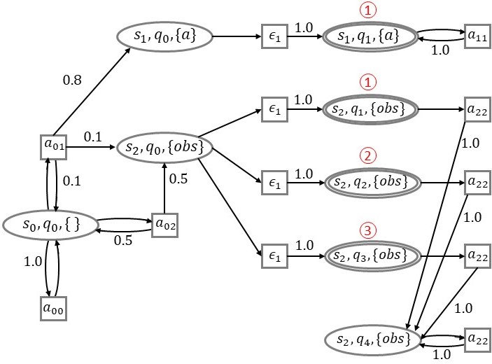
(a)

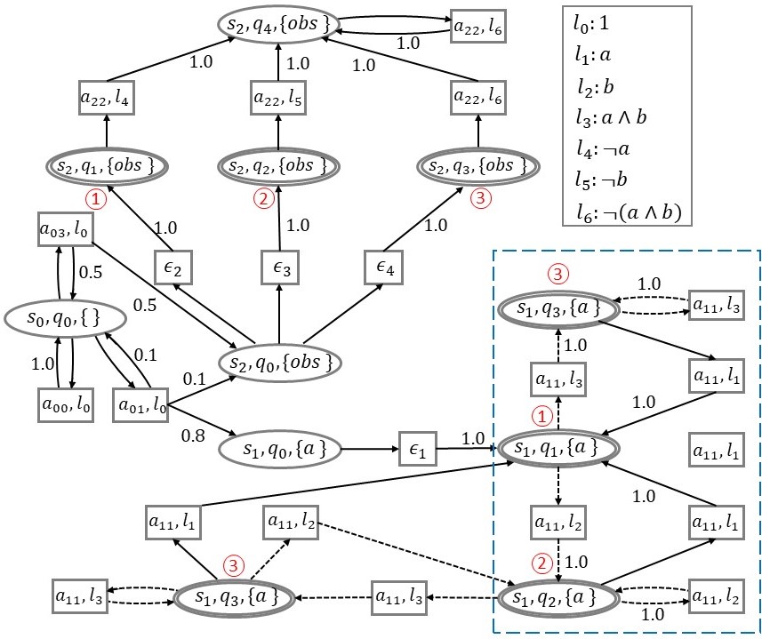
(b)

      

Figure 2: Two different product MDPs between the PL-MDP and the LDGBA provided in Fig. 1. (a) Standard product MDP. There are no criteria to evaluate a policy for task satisfaction, and we can not find a path satisfying the acceptance condition. (b) Partial structure of the relaxed product MDP. $l_{i},\forall i\in\left\{0,1,\ldots,7\right\}$ denotes the input alphabet of each automaton transition as shown in the gray rectangular. The gray dashed lines represent the transitions with nonzero violation costs, and the graph component in blue rectangular contains the path that satisfies the acceptance condition.

Example 2.

Fig. 2 (a) and (b) provide examples of a standard product MDP and the corresponding relaxed one, respectively, to illustrate the benefits of designing the relaxed product MDP. Both product MDPs are constructed between the PL-MDP and the LDGBA of LTL formula $\phi=\oblong\lozenge\mathtt{a}\land\oblong\lozenge\mathtt{b}$, as shown in Fig. 1. Obviously, the product MDP in Fig. 2 (a) has no AMEC, while the relaxed product MDP in Fig. 2 (b) has one AMEC (blue rectangular) intersecting with all accepting sets. Moreover, the transitions with nonzero violation costs are gray dashed lines. Note that due to the complicated graph structure, we use the LDGBA in this example to illustrate the novelty of the proposed relaxed product MDP. Its advantages for infeasible cases are also applicable to the E-LDGBA.

Given a relaxed product MDP $\mathcal{\overline{\mathcal{R}}}$, let $MC_{\overline{\mathcal{R}}}^{\pi}$ denote the Markov chain induced by the policy $\pi$ on $\mathcal{\overline{\mathcal{R}}}$, whose states can be represented by a disjoint union of a transient class $T_{\pi}$ and $n$ closed irreducible recurrent sets $R_{\pi}^{j}$, $j\in\left\{1,\ldots,n\right\}$, i.e., $MC_{\overline{\mathcal{R}}}^{\pi}=T_{\pi}\sqcup R_{\pi}^{1}\sqcup R_{\pi}^{2}\ldots R_{\pi}^{n}$ [35].

Lemma 3.

Given a relaxed product MDP $\mathcal{\overline{\mathcal{R}}=M}\otimes\mathcal{\overline{A}}_{\phi}$ , the recurrent class $R_{\pi}^{j}$ of $MC_{\overline{\mathcal{R}}}^{\pi}$, $\forall j\in\left\{1,\ldots,n\right\}$, induced by $\pi$ satisfies one of the following conditions:

1. $R_{\pi}^{j}\cap F_{i}^{\overline{\mathcal{R}}}\neq\emptyset,\forall i\in\left\{1,\ldots f\right\}$, or

2. $R_{\pi}^{j}\cap F_{i}^{\overline{\mathcal{R}}}=\emptyset,\forall i\in\left\{1,\ldots f\right\}$.

Proof.

The following proof is based on contradiction. Assume there exists a policy such that $R_{\pi}^{j}\cap F_{k}^{\overline{\mathcal{R}}}\neq\emptyset$, $\forall k\in K$, where $K$ is a subset of $2^{\left\{1,\ldots f\right\}}\setminus\left\{\left\{1,\ldots f\right\},\emptyset\right\}$. As discussed in [35], for each state in recurrent class, it holds that $\stackrel{{\scriptstyle[}}{{n}}=0]{\infty}{\sum}p^{n}(x,x)=\infty$, where $x\in R_{\pi}^{j}\cap F_{k}^{\overline{\mathcal{R}}}$ and $p^{n}(x,x)$ denotes the probability of returning from a transient state $x$ to itself in $n$ steps. This means that each state in the recurrent class occurs infinitely often. However, based on the embedded tracking frontier function of E-LDGBA in Def. 9, the tracking set $T$ will not be reset until all accepting sets have been visited. As a result, neither $\overline{q}_{k}\in\overline{F}_{k}$ nor $x_{k}=(s,\overline{q}_{k})\in R_{\pi}^{j}\cap F_{k}^{\overline{\mathcal{R}}}$ with $s\in S$ will occur infinitely, which contradicts the property $\stackrel{{\scriptstyle[}}{{n}}=0]{\infty}{\sum}p^{n}(x_{k},x_{k})=\infty$. ∎

Lemma 3 indicates that, for any policy, all accepting sets will be placed either in the transient class or the recurrent class. As a result, the issue of NMEC, as in many existing methods, can be avoided. Based on Theorem 1 and Lemma 3, Problem 1 can be reformulated as follows.

Problem 2.

Given a user-specified LTL task $\phi$ and an MDP with unknown transition probabilities (i.e., motion uncertainties) and unknown labeling probabilities (i.e., environment uncertainties), the objective is to find a policy in decreasing order of priority to 1) satisfy the acceptance condition of the relaxed product MDP, and 2) reduce the violation cost of the expected return.

V Learning-Based Control Synthesis

In this section, RL is leveraged to identify policies for Problem 2. Specifically, a model-free multi-objective RL (MORL) is designed.

V-A Reward Design

The accepting reward function $\varLambda:X\shortrightarrow\mathbb{R}$ is designed as

$$\varLambda(x)=\left\{\begin{array}[]{cc}r_{\varLambda}&\text{ if $\exists$i$\in\left\{1,\ldots f\right\}$ such that $x\in F_{i}^{\overline{\mathcal{R}}}$ },\\ 0&\text{ otherwise},\end{array}\right.$$ (7)

where $r_{\varLambda}>0$. The violation function $V:X\times U^{\overline{\mathcal{R}}}\times X\shortrightarrow\mathbb{R}$ is designed as

$$V(x,u^{\overline{\mathcal{R}}},x^{\prime})=-c_{V}^{\overline{\mathcal{R}}}(x,u^{\overline{\mathcal{R}}},x^{\prime}).$$ (8)

The non-negative $\varLambda(x)$ enforces the accepting condition of $\mathcal{\overline{\mathcal{R}}}$, while the non-positive function $V(x,u^{\overline{\mathcal{R}}},x^{\prime})$ indicates the penalty of violations. Let $\boldsymbol{U}_{\boldsymbol{\pi}}=\left[\begin{array}[]{ccc}U_{\boldsymbol{\pi}}(x_{0})&U_{\boldsymbol{\pi}}(x_{1})&\ldots\end{array}\right]^{T}\in\mathbb{R}^{N}$ denote the stacked expected return induced by $\boldsymbol{\pi}$ over $\mathcal{\overline{\mathcal{R}}}$ with $N=\left|X\right|$, the expected return is designed as

$$\boldsymbol{U}=\stackrel{{\scriptstyle[}}{{n}}=0]{\infty}{\sum}\gamma^{n}\boldsymbol{P}_{\boldsymbol{\pi}}^{n}(\boldsymbol{\varLambda}_{\boldsymbol{\pi}}+\beta\boldsymbol{V}_{\boldsymbol{\pi}}\cdot\mathbf{1}_{N}),$$ (9)

where $0<\gamma<1$ is a discount factor, $\boldsymbol{P}_{\boldsymbol{\pi}}\in\mathbb{R}^{N\times N}$ is a matrix with entries representing the probabilities $p^{\overline{\mathcal{R}}}(x,\boldsymbol{\pi}(x),x^{\prime})$ under $\pi$ for all $x,x^{\prime}\in X$, $\boldsymbol{\varLambda}_{\boldsymbol{\pi}}=\left[\begin{array}[]{ccc}\varLambda(x_{0})&\varLambda(x_{1})&\ldots\end{array}\right]^{T}\in\mathbb{R}^{N}$ is the stacked state rewards, $\beta\in\mathbb{R}^{+}$ is a weight indicating the relative importance, $\mathbf{1}_{N}$ is an $N$-dimensional vector of ones, and $\boldsymbol{V}_{\boldsymbol{\pi}}=\boldsymbol{P}_{\boldsymbol{\pi}}\circ\boldsymbol{V}\in\mathbb{R}^{N\times N}$ is the Hadamard product of $\boldsymbol{P}_{\boldsymbol{\pi}}$ and $\boldsymbol{V}$, i.e., $\boldsymbol{V}_{\boldsymbol{\pi}}=$$\left[p^{\overline{\mathcal{R}}}(x,a_{\boldsymbol{\pi}}(x),x^{\prime})\cdotp V(x,u^{\overline{\mathcal{R}}},x^{\prime})\right]_{N\times N}$ and $a_{\boldsymbol{\pi}}(x)$ represents taking action at $x$ from policy $\boldsymbol{\pi}$.

The objective is to identify a stationary policy $\pi^{*}$ that maximizes the expected return

$$\pi^{*}=\underset{\pi}{\arg\max}\stackrel{{\scriptstyle[}}{{n}}=0]{\infty}{\sum}\gamma^{n}\boldsymbol{P}_{\boldsymbol{\pi}}^{n}(\boldsymbol{\varLambda}_{\boldsymbol{\pi}}+\beta\boldsymbol{V}_{\boldsymbol{\pi}}\cdot\mathbf{1}_{N})$$ (10)

$U_{\boldsymbol{\pi}}(x)\leq U_{\boldsymbol{\pi}^{*}}(x)$ for all $x\in X$ if $\pi^{*}$ in (10) is optimal.

Theorem 2.

Consider a relaxed MDP product $\mathcal{\overline{\mathcal{R}}=M}\otimes\mathcal{\overline{A}}_{\phi}$. If there exists a policy $\boldsymbol{\bar{\pi}}$ such that an induced run $r_{\overline{\mathcal{P}}}^{\boldsymbol{\bar{\pi}}}$ satisfies the acceptance condition of $\overline{\mathcal{R}}$, any optimization method that solves (10) can find the policy $\boldsymbol{\bar{\pi}}$.

Proof.

Detailed rigorous analysis can be found in appendixA ∎

To solve Problem 2 by optimizing the expected return of (9), $r_{\varLambda}$, $\beta$ ,$\gamma$ can be determined as follows. Firstly, we can choose a fixed $r_{\varLambda}$. Then, $\gamma$ can be obtained by solving (21) and (22). Finally, the range of $\beta$ can be determined by solving (18) and (22). In order to minimize the violation cost, a great value of $\beta$ is preferred.

Algorithm 3 Model-free RL-based control on MDPs under potentially soft LTL specifications.

1:procedure Input: ($\mathcal{M}$ , $\phi$, $\varLambda$) Output: optimal policy $\boldsymbol{\pi}^{*}$ Initialization: Set $episode=0$ , $iteration=0$ and
                         $\tau$ as maximum allowed learning steps

2:     Initialize $r_{\varLambda}$, $\beta$ ,$\gamma$;

3:     for  all $x\in X$  do

4:         $U(x)=0$ and $Q(x,u^{\mathcal{\mathcal{\mathcal{\mathcal{\overline{\mathcal{R}}}}}}})=0$ $\forall x$, $u^{\mathcal{\mathcal{\mathcal{\mathcal{\overline{\mathcal{R}}}}}}}\in U^{\overline{\mathcal{R}}}(x)$

5:         $Count(x,u^{\mathcal{\mathcal{\mathcal{\mathcal{\overline{\mathcal{R}}}}}}})=0$ for all $u^{\mathcal{\mathcal{\mathcal{\overline{\mathcal{R}}}}}}\in U^{\overline{\mathcal{R}}}(x)$

6:     end for

7:     $x=x_{0}$;

8:     while  $\boldsymbol{U}$ are not converged  do

9:         $episode++$;

10:         $\epsilon=1/episode$;

11:         while $iteration<\tau$  do

12:              $iteration++$

13:              $u=\underset{u^{\overline{\mathcal{R}}}\in U^{\overline{\mathcal{R}}}}{\arg\max}Q(x,u^{\overline{\mathcal{R}}})$ with probability
              $1-\epsilon$, or select $u$ randomly from $U^{\overline{\mathcal{R}}}(x)$

14:              Obtain and execute $a$ of $\mathcal{M}$ from $u$

15:              Observe $x^{\prime}$, $\varLambda(x)$,$c_{V}^{\overline{\mathcal{R}}}(x,u,x^{\prime})$

16:              $r\text{$\leftarrow$}\varLambda(x)-\beta c_{V}^{\overline{\mathcal{R}}}(x,u,x^{\prime})$

17:              $Count(x,u)++$

18:              $\alpha=1/Count(x,u)$

19:              $Q(x,u)\text{$\leftarrow$}(1-\alpha)Q(x,u)+\newline \hskip 46.00012pt\alpha\left[r+\gamma\cdot\underset{u^{\overline{\mathcal{R}}}\in U^{\overline{\mathcal{R}}}}{\max}Q(x^{\prime},u^{\overline{\mathcal{R}}})\right]$

20:              $x=x^{\prime}$

21:         end while

22:     end while

23:     for  all $x\in X$  do

24:         $U(x)=\underset{u^{\mathcal{\mathcal{\mathcal{\mathcal{\overline{\mathcal{R}}}}}}}\in U^{\mathcal{\mathcal{\overline{\mathcal{R}}}}}}{\max}Q(x,u^{\mathcal{\mathcal{\mathcal{\mathcal{\overline{\mathcal{R}}}}}}})$

25:         $\boldsymbol{\pi}^{*}(x)=\underset{u^{\mathcal{\mathcal{\mathcal{\mathcal{\overline{\mathcal{R}}}}}}}\in U^{\mathcal{\mathcal{\overline{\mathcal{R}}}}}}{\arg\max}U(x)$

26:     end for

27:end procedure

Remark 2.

Problem 2 is a MORL problem, and Theorem 2 shows how it can be addressed to ensure acceptance satisfaction while trying to minimize the long-term violation. In literature, MORL based approaches often seek to identify Pareto fronts [36]. However, our problem considers a trade-off between two possibly conflicting objectives. There are no existing MORL methods to provide formal guarantee of both acceptance satisfaction and violation depreciation, which might result in a safety issue during the execution of optimal policies. To overcome this challenge, we can always divide the task into two parts: hard and soft constraints, with two parallel automatons. The hard task should always be satisfied, and it can be applied with the traditional product MDP as Def. 10. The soft part can be partially infeasible, and it can be relaxed as Def. 11. Such an idea can be found in our previous results [12].

It is worth pointing out that $\boldsymbol{V}_{\pi}$ is a sparse matrix because most transitions have zero violation cost, and Theorem 2 provides a performance guarantee for the worst cases of $\beta$ for acceptance satisfaction. By applying E-LDGBA, the sparse reward issue can be improved compared with using LDGBA.

V-B Model-Free Reinforcement Learning 

Q-learning is a model-free RL method [14], which can be used to find the optimal policy for a finite MDP. In particular, the agent updates its Q-value from $x$ to $x^{\prime}$ according to

$$Q(x,u^{\overline{\mathcal{R}}})\text{$\leftarrow$} (1-\alpha)Q(x,u^{\overline{\mathcal{R}}})$$ (11)

$$+\alpha\left[R(x,u^{\overline{\mathcal{R}}},x^{\prime})+\gamma\underset{u_{*}^{\overline{\mathcal{R}}}\in U^{\overline{\mathcal{R}}}(x)}{\max}Q(x,u_{*}^{\overline{\mathcal{R}}})\right],$$

where $Q(x,u^{\overline{\mathcal{R}}})$ is the Q-value of the state-action pair $(x,u^{\overline{\mathcal{R}}})$, $\alpha\in(0,1)$ is the learning rate, $0<\gamma\leq 1$ is the discount factor, and

$$R(x,u^{\overline{\mathcal{R}}},x^{\prime})=\varLambda(x)+\beta V(x,u^{\overline{\mathcal{R}}},x^{\prime})$$ (12)

denotes the immediate reward from $x$ to $x^{\prime}$ under $u^{\overline{\mathcal{R}}}$. The learning strategy is outlined in Alg. 3 that shows the steps of applying Q-learning into our framework. By applying the off-the-shelf RL, we have the following theorem.

Theorem 3.

Given a finite MDP, i.e., $\overline{\mathcal{R}}=\mathcal{M}\otimes\mathcal{\overline{A}}_{\phi}=(X,U^{\overline{\mathcal{R}}},p^{\overline{\mathcal{R}}},x_{0},F^{\overline{\mathcal{R}}},c_{V}^{\overline{\mathcal{R}}},f_{V},T)$, let $Q^{*}(x,u^{\overline{\mathcal{R}}})$ be the optimal Q-function for every pair of state-action $(x,u^{\overline{\mathcal{R}}})$. Consider the RL with the updating rule

$$Q_{k+1}(x,u^{\overline{\mathcal{R}}})\text{$\leftarrow$} (1-\alpha_{k})Q_{k}(x,u^{\overline{\mathcal{R}}})+$$

$$\alpha_{k}\left[R(x,u^{\overline{\mathcal{R}}},x^{\prime})+\gamma\underset{u_{*}^{\overline{\mathcal{R}}}\in U^{\overline{\mathcal{R}}}(x)}{\max}Q_{k}(x,u_{*}^{\overline{\mathcal{R}}})\right],$$

where $k$ is the updating step, $\gamma\in(0,1]$ is the discount factor, and the learning rate $\alpha_{k}$ satisfies $\underset{k}{\sum\alpha_{k}}=\infty$ and $\underset{k}{\sum\alpha^{2}_{k}}<\infty$. Then, $Q_{k}(x,u^{\overline{\mathcal{R}}})$ converges to $Q^{*}(x,u^{\overline{\mathcal{R}}})$ with a probability of $1$ as $k\rightarrow\infty$.

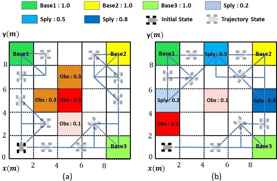
Figure 3: Simulated trajectories of 50 time steps under corresponding optimal policies in feasible workspaces with (a) a simple task, i.e., $\varphi_{case1}$, and (b) a relatively complex task, i.e., $\varphi_{case2}$.

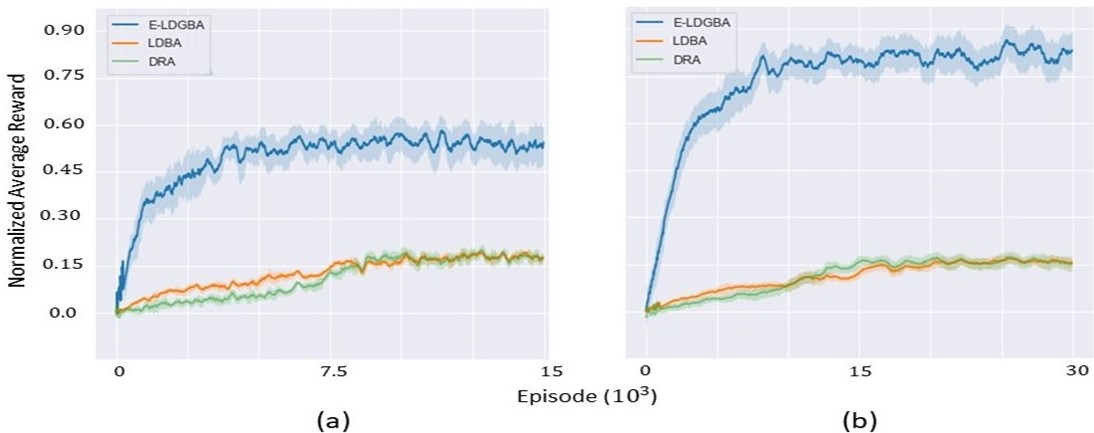
Figure 4: Normalized average rewards during training using E-LDGBA, LDBA, and DRA for (a) Task $\varphi_{case1}$ in Fig. 3 and (b) Task $\varphi_{case2}$ in Fig. 3.

Theorem 3 is an immediate result of [37]. With standard learning rate $\alpha$ and discount factor $\gamma$ as Alg. 3, Q-value will converge to a unique limit $Q^{*}$. Therefore, the optimal expected utility and policy can be obtained as $U_{\boldsymbol{\pi}}^{*}(x)=\underset{u^{\overline{\mathcal{R}}}\in U^{\overline{\mathcal{R}}}(x)}{\max}Q^{*}(x,u^{\overline{\mathcal{R}}})$ and $\boldsymbol{\pi}^{*}(x)=\underset{u^{\overline{\mathcal{R}}}\in U^{\overline{\mathcal{R}}}(x)}{\arg\max}Q^{*}(x,u^{\overline{\mathcal{R}}})$. In (11), the discount $\gamma$ is tuned to improve the trade-off between immediate and future rewards. Note that our novel design can be also applied with modern advanced RL algorithms.

Complexity Analysis The number of states is $\left|S\right|\times\left|Q\right|$, where $\left|Q\right|$ is determined by the original LDGBA $\mathcal{A}_{\phi}$ because the construction of E-LDGBA $\mathcal{\overline{A}}_{\phi}$ will not increase the size, and $\left|S\right|$ is the size of the labeled MDP model. Due to the consideration of a relaxed product MDP and extended actions in Def. 11, the maximum complexity of actions available at $x=(s,l,q)$ is $O(\left|A(s)\right|\times(\left|\Sigma\right|+1))$, since $U^{\overline{\mathcal{R}}}(x)$ are created from $A(s)$ and $\Sigma\cup\left\{\epsilon\right\}$.

VI Case Studies

The developed RL-based control synthesis is implemented in Python. Owl [34] is used to convert LTL specifications into LDGBA, and P_MDP package[8] is used to construct state transition models. All simulations are carried out on a laptop with 2.60 GHz quad-core CPU and 8 GB of RAM. For Q-learning, the optimal policies of each case are generated using $10^{5}$ episodes with random initial states. The learning rate $\alpha$ is determined by Alg. 3 with $\gamma=0.999$ and $r_{\varLambda}=10$. To validate the effectiveness of our approach, we first carry out simulations over grid environments and then validate the approach in a more realistic office scenario with a TIAGo robot.

VI-A Simulation Results

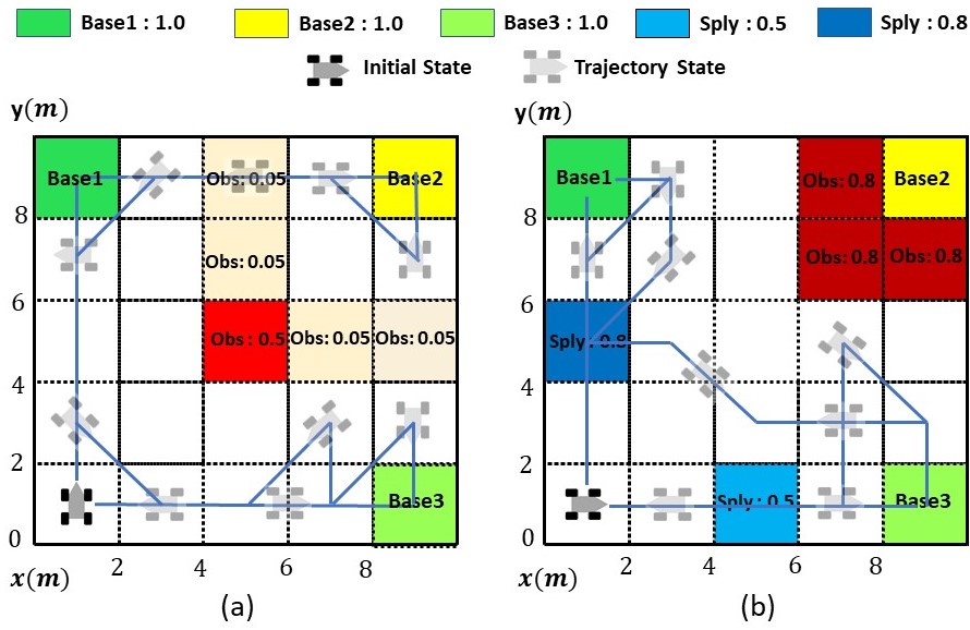
Figure 5: Simulated trajectories of 50 time steps under corresponding optimal policies for partially infeasible tasks on workspaces where the agent visits the grid labeled as Base2 with (a) a low risk or (b) a high risk.

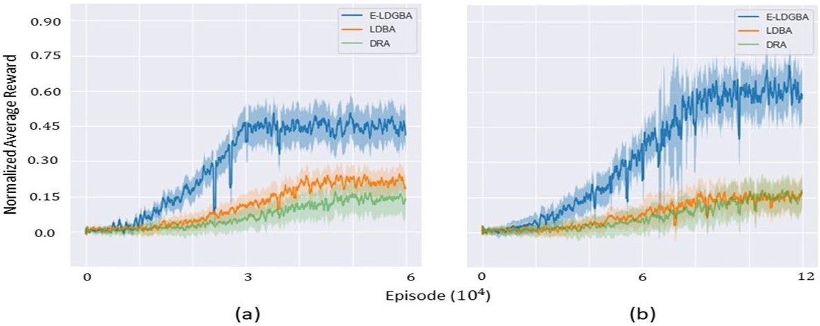
Figure 6: Normalized average rewards during training using E-LDGBA, LDBA, and DRA for Task $\varphi_{case3}$ on two environments in Fig. 5, respectively.

Consider a partitioned $10m\times 10m$ workspace, as shown in Fig. 3 and Fig. 5, where each cell is a $2m\times 2m$ area. The cells are marked with different colors to represent various areas of interest, including $\mathtt{Base}1,\mathtt{Base}2,\mathtt{Base}3,\mathtt{Obs}$, and $\mathtt{Sply}$, where $\mathtt{Obs}$ and $\mathtt{Sply}$ are shorthands for obstacle and supply, respectively. To model environment uncertainties, the number associated with a cell represents the likelihood that the corresponding property appears at that cell. For example, $\mathtt{Obs}:0.1$ indicates the obstacles occupy this cell with a probability of 0.1. The robot dynamics follow the unicycle model, i.e., $\dot{x}=v\cdot\sin(\theta)$, $\dot{y}=v\cdot\cos(\theta)$, and $\dot{\theta}=\omega$, where $x,y,\theta$ indicate the robot positions and orientation. The linear and angular velocities are the control inputs, i.e., $u=(v,\omega)$.

In addition, we assume the robot cannot consistently successfully execute the action primitives to model motion uncertainties. For instance, action primitives “$FR$” and “$BK$” mean the robot can successfully move forward and backward $2m$ with a probability of $0.9$, respectively, and fail with a probability of $0.1$. On the other hand, action primitives “$TR$” and “$TL$” mean the robot can successfully turn right and left for an angle of $\frac{\pi}{2}$ exactly with a probability of $0.9$, respectively, and fail by an angle of $\frac{\pi}{4}$ (undershoot) with a probability of $0.05$ and an angle of $\frac{3\pi}{4}$ (overshoot) with another probability of $0.05$. Fianlly, action primitive “$ST$” means the robot remains at its current cell. The resulting MDP model has $25$ states.

Case 1: As shown in Fig. 3 (a), we first consider a case in which user-specified tasks can be successfully executed. The desired surveillance task to be performed is formulated as

$$\varphi_{case1}=(\oblong\lozenge\mathtt{Base}1)\land(\oblong\lozenge\mathtt{Base}2)\land(\oblong\lozenge\mathtt{Base}3)\land\oblong\lnot\mathtt{Obs},$$ (13)

which requires the mobile robot to visit all base stations infinitely while avoiding obstacles. Its corresponding LDGBA has $2$ states with $3$ accepting sets, and the relaxed product MDP has $50$ states. In this case, each episode terminates after $\tau=100$ steps and $\beta=8$. Fig. 3 (a) shows the generated optimal trajectory, which indicates $\varphi_{case1}$ is completed.

Case 2: We validate our approach with more complex task specifications in Fig. 3 (b). The task is expressed as

$$\varphi_{case2}=\varphi_{case1}\land\oblong\lozenge(\mathtt{Sply}\rightarrow\varbigcirc((\lnot\mathtt{Sply})\mathcal{U}\mathtt{\varphi_{one1}})),$$ (14)

where $\varphi_{one1}=\mathtt{Base}1\lor\mathtt{Base}2\lor\mathtt{Base}3$. $\varphi_{case2}$ requires the robot to visit the supply station and then go to one of the base stations while avoiding obstacles. It also requires all base stations to be visited. Its corresponding LDGBA has $24$ states with $4$ accepting sets, and the relaxed product MDP has $600$ states. The generated optimal trajectory is shown in Fig. 3 (b).

Case 3: We consider more challenging workspaces in Fig. 5 (a) and (b), where user-specified tasks might not be fully feasible due to potential obstacles (i.e., environment uncertainties). The task specification is

$$\varphi_{case3}=\varphi_{case1}\land\oblong\lozenge(\varphi_{one1}\rightarrow\varbigcirc((\lnot\varphi_{one1})\mathcal{U}\mathtt{Sply})),$$ (15)

where $\varphi_{case3}$ requires the robot to visit one of the base stations and then go to one of the supply stations while avoiding obstacles. Its corresponding LDGBA has $24$ states with $4$ accepting sets, and the product-MDP has $600$ states.

For $\varphi_{case2}$ and $\varphi_{case3}$, each episode terminates after $\tau=1000$ steps and $\beta=5$. Note that in the case of Fig. 5 (a) and (b), AMECs might not exist since $\mathtt{Base}2$ is surrounded by probabilistic obstacles and may not be visited. The simulated optimal trajectories indicate that the robot takes a risk to accomplish the task in the case of Fig. 5 (a). In contrast, the robot decides not to visit $\mathtt{Base}2$ to avoid the high risk of running into obstacles in the case of Fig. 5 (b).

Scalability Analysis: The RL-based policy synthesis is performed for $\varphi_{case1}$ over workspaces of various sizes (each grid is further partitioned) to show the computational complexity. The simulation results are listed in Table I. The number of episodes in Table I indicates the time used to converge to optimal satisfaction planing. It is also verified that the given task $\varphi_{case1}$ can be successfully carried out in large workspaces.

Table I: Simulation results of large scale workspaces

Workspace	MDP	$\overline{\mathcal{R}}$	Episode
size[cell]	States	States	Steps
$15\times 15$	225	450	30000
$25\times 25$	625	1250	50000
$40\times 40$	1600	3200	100000

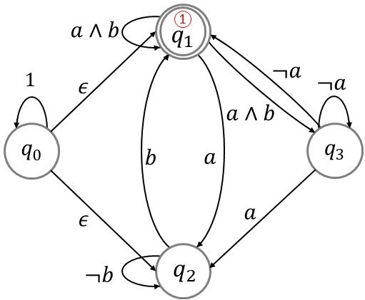
(a)

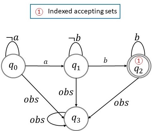
(b)

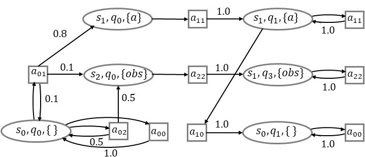
(c)

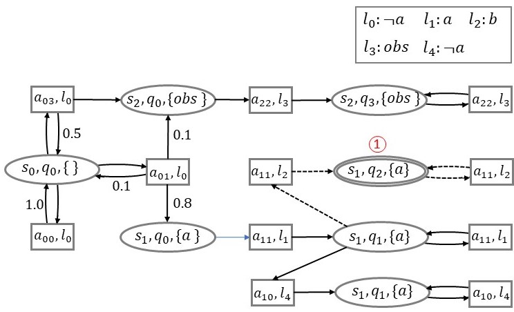
(d)

             

Figure 7: Examples of the baseline comparisons regarding automaton structures and infeasible cases. (a) The LDBA of the LTL formula $\phi=\oblong\lozenge\mathtt{a}\land\oblong\lozenge\mathtt{b}$ only has one accepting set. (b) The LDGBA of the LTL formula $\phi=\lozenge(\mathtt{a}\land\lozenge\mathtt{b})$. (c) The standard product MDP between the PL-MDP in Fig. 1 (a) and the LDGBA of the LTL formula $\phi=\lozenge(\mathtt{a}\land\lozenge\mathtt{b})$ in Fig. 7 (b). There are no accepting states, and this is an infeasible case. (d) The relaxed product MDP (Def. 11) corresponding to the standard product MDP in (c). An accepting state exists, and the dashed arrows represent the transitions with nonzero violation costs.

VI-B Experimental Results

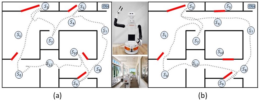
Figure 8: Experimental trajectories for the task $\varphi_{case4}$.

This section verifies our algorithm for high-level decision-making problems in a real-world environment and shows that the framework can be adopted with low-level noisy controllers to formulate a hierarchical architecture. Consider an office environment constructed in ROS Gazebo, as shown in Fig 8, which consists of $7$ rooms denoted by $S_{0},S_{2},S_{3},S_{5},S_{9},S_{10},\mathtt{Obs}$ and $5$ corridors denoted by $S_{1},S_{4},S_{7},S_{8},S_{12}$. The TIAGo robot can follow a collision-free path from the center of one region to another without crossing other regions using obstacle-avoidance navigation. To model motion uncertainties, it is assumed that the robot can successfully follow its navigation controller by moving to the desired region with a probability of $0.9$ and fail by moving to an adjacent region with a probability of $0.1$. The resulting MDP has $12$ states. The service to be performed by TIAGo is expressed as

$$\varphi_{case4}=\varphi_{all}\land\oblong\lnot\mathtt{Obs}$$ (16)

where $\varphi_{all}=\oblong\lozenge S_{0}\land\oblong\lozenge S_{2}\land\oblong\lozenge S_{3}\land\oblong\lozenge S_{5}\land\oblong\lozenge S_{9}\land\oblong\lozenge S_{10}$. In (16), $\varphi_{all}$ requires the robot to always service all rooms (e.g., pick trash) and return to $S_{0}$ (e.g., release trash) while avoiding $\mathtt{Obs}$. Its corresponding LDGBA has $6$ states with $6$ accepting sets, and the relaxed product MDP has $72$ states.

All room doors are open, except the doors of room $S_{5}$ $S_{10}$ in Fig. 8 (b). As a result, $\varphi_{case4}$ can not be fully completed in the case of Fig. 8 (b), and the task is infeasible. It is also worth pointing out there do not exist AMECs in the corresponding product automaton $\overline{\mathcal{P}}$ or $\mathcal{\overline{\mathcal{P}}}$ in Fig. 8 (a) because the robot has the nonzero probability of entering $Obs$ at state $S_{7}$ as the motion uncertainties arise. The optimal policies for the two cases are generated, and each episode terminates after $\tau=150$ steps with $\beta=4$. The generated satisfying trajectories (without collision) of one round are shown in Fig. 8 (a) and (b), and the robot tries to complete the feasible part of task $\varphi_{case4}$ in Fig. 8 (b).

VII Conclusions

This paper presents a learning-based control synthesis of motion planning subject to motion and environment uncertainties. The LTL formulas are applied to express complex tasks via the automaton theory. Differently, in this work, an LTL formula is converted into a designed E-LDGBA to improve the performance of mission accomplishment and resolve the drawbacks of DRA and LDBA. Furthermore, the innovative relaxed product MDP and utility schemes consisting of the accepting reward and violation reward are proposed to accomplish the satisfaction of soft tasks. In order to provide formal guarantees of achieving the goals of multi-objective optimizations, future research will consider more advanced multi-objective learning methods. Also problems over continuous state and/or action spaces will be studied by incorporating deep neural networks.

Appendix A Proof of Theorem 2

For any policy $\boldsymbol{\pi}$, let $MC_{\overline{\mathcal{R}}}^{\boldsymbol{\pi}}$ denote the Markov chain induced by $\pi$ on $\overline{\mathcal{R}}$. Since$MC_{\overline{\mathcal{R}}}^{\boldsymbol{\pi}}$ can be written as $MC_{\overline{\mathcal{R}}}^{\boldsymbol{\pi}}=T_{\boldsymbol{\pi}}\sqcup R_{\boldsymbol{\pi}}^{1}\sqcup R_{\boldsymbol{\pi}}^{2}\ldots R_{\boldsymbol{\pi}}^{n}$, (9) can be reformulated as

$$\left[\begin{array}[]{c}\boldsymbol{U}_{\boldsymbol{\pi}}^{tr}\\ \boldsymbol{U}_{\boldsymbol{\pi}}^{rec}\end{array}\right]= \stackrel{{\scriptstyle[}}{{n}}=0]{\infty}{\sum}\gamma^{n}\left[\begin{array}[]{cc}\boldsymbol{P}_{\pi}\left(\mathcal{T},\mathcal{T}\right)&\boldsymbol{P}_{\boldsymbol{\pi}}^{tr}\\ \boldsymbol{0}_{\sum_{i=1}^{m}N_{i}\times r}&\boldsymbol{P}_{\boldsymbol{\pi}}\left(R,R\right)\end{array}\right]^{n}$$ (17)

$$\cdot\left(\left[\begin{array}[]{c}\boldsymbol{\varLambda}_{\boldsymbol{\pi}}^{tr}\\ \boldsymbol{\varLambda}_{\boldsymbol{\pi}}^{rec}\end{array}\right]+\beta\left[\begin{array}[]{c}\boldsymbol{\boldsymbol{O}}_{\boldsymbol{\pi}}^{tr}\\ \boldsymbol{\boldsymbol{O}}_{\boldsymbol{\pi}}^{rec}\end{array}\right]\right),$$

where $\boldsymbol{U}_{\boldsymbol{\pi}}^{tr}$ and $\boldsymbol{U}_{\boldsymbol{\pi}}^{rec}$ are the utilities of states in the transient and recurrent classes, respectively. In (17), $\boldsymbol{P}_{\boldsymbol{\pi}}\left(\mathcal{T},\mathcal{T}\right)\in\mathbb{R}^{r\times r}$ denotes the probability transition matrix between states in $T^{\boldsymbol{\pi}}$. $\boldsymbol{P}_{\pi}^{tr}=\left[\boldsymbol{P}_{\pi}^{tr_{1}}\ldots\boldsymbol{P}_{\pi}^{tr_{m}}\right]\in\mathbb{R}^{r\times\sum_{i=1}^{m}N_{i}}$ is a probability transition matrix where $\boldsymbol{P}_{\pi}^{tr_{i}}\mathbb{\in R}^{r\times N_{i}}$ represents the probability of transiting from a transient state in $T^{\pi}$ to the states of $R_{\pi}^{i}$. The $\boldsymbol{P}_{\boldsymbol{\pi}}\left(R,R\right)$ is a diagonal block matrix, where the $i$th block is an $N_{i}\times N_{i}$ matrix containing transition probabilities between states within $R_{\boldsymbol{\pi}}^{j}$. $\boldsymbol{P}^{\boldsymbol{\pi}}\left(\overline{\mathcal{R}},\overline{\mathcal{R}}\right)$ is a stochastic matrix since each block matrix is a stochastic matrix [35]. The rewards vector $\boldsymbol{\varLambda}_{\boldsymbol{\pi}}$ can also be partitioned to $\boldsymbol{\varLambda}_{\boldsymbol{\pi}}^{tr}$ and $\boldsymbol{\varLambda}_{\boldsymbol{\pi}}^{rec}$. Similarly, $\boldsymbol{\boldsymbol{O}}_{\boldsymbol{\pi}}=\left[\begin{array}[]{ccc}O_{\boldsymbol{\pi}}\left(x_{0}\right)&O_{\boldsymbol{\pi}}\left(x_{1}\right)&\ldots\end{array}\right]^{T}=\boldsymbol{V}_{\boldsymbol{\pi}}\cdot\mathbf{1}_{N}$ can be divided into transient class $\boldsymbol{\boldsymbol{O}}_{\boldsymbol{\pi}}^{tr}$ and recurrent class $\boldsymbol{\boldsymbol{O}}_{\boldsymbol{\pi}}^{rec}$.

We prove this theorem by contradiction. Suppose there exists an optimal policy $\pi^{*}$ not satisfying the acceptance condition of $\overline{\mathcal{R}}$. Based on Lemma 3, the following is true: $F_{k}^{\overline{\mathcal{R}}}\subseteq T_{\boldsymbol{\pi}^{*}},\forall i\in\left\{1,\ldots f\right\}$. As a result, for any $j\in\left\{1,\ldots n\right\}$, we have $R_{\boldsymbol{\pi}^{*}}^{j}\cap F_{i}^{\overline{\mathcal{R}}}\neq\emptyset,\forall i\in\left\{1,\ldots f\right\}$.

The strategy is to show that there always exists a policy $\bar{\pi}$ with greater utility than $\boldsymbol{\pi}^{*}$, which contradicts to the optimality of $\pi^{*}$. Let’s consider a state $x_{R}\in R_{\boldsymbol{\pi}^{*}}^{j}$ and let $\boldsymbol{P}_{\boldsymbol{\pi}^{*}}^{x_{R}R_{\pi^{*}}^{j}}$ denote a row vector of $\boldsymbol{P}_{\boldsymbol{\pi}^{*}}^{n}\left(R,R\right)$ that contains the transition probabilities from $x_{R}$ to the states in the same recurrent class $R_{\boldsymbol{\pi}^{*}}^{j}$ in $n$ steps. The expected return $U_{\boldsymbol{\pi}^{*}}\left(x_{R}\right)$ of $x_{R}$ under $\boldsymbol{\pi}^{*}$ is then obtained from (17) as: $U_{\boldsymbol{\pi}^{\boldsymbol{*}}}^{rec}\left(x_{R}\right)=\stackrel{{\scriptstyle[}}{{n}}=0]{\infty}{\sum}\gamma^{n}\left[\boldsymbol{0}_{k_{1}}^{T}\>\boldsymbol{P}_{\boldsymbol{\pi}^{*}}^{x_{R}R_{\boldsymbol{\pi}^{*}}^{j}}\boldsymbol{0}_{k_{2}}^{T}\right]\left(\boldsymbol{\varLambda}_{\boldsymbol{\pi}^{*}}^{rec}+\beta\boldsymbol{O}_{\boldsymbol{\pi}^{*}}^{rec}\right)$ where $k_{1}=\sum_{i=1}^{j-1}N_{i}$, $k_{2}=\sum_{i=j+1}^{n}N_{i}$. Since $\overline{\mathcal{R}}_{\boldsymbol{\pi}^{*}}^{j}\cap F_{i}^{\overline{\mathcal{R}}}=\emptyset,\forall i\in\left\{1,\ldots f\right\}$, all the elements of $\boldsymbol{\varLambda}_{\boldsymbol{\pi}^{*}}^{rec}$ are equal to zero and each entry of $\boldsymbol{O}_{\pi^{*}}^{rec}$ is non-positive. We can conclude $U_{\pi^{*}}^{rec}\left(x_{R}\right)\leq 0$. To prove that optimal policy $\pi^{*}$ raises a contradiction, the following analysis will show that $U_{\boldsymbol{\bar{\pi}}}^{rec}\left(x_{R}\right)\geq U_{\boldsymbol{\pi}^{*}}^{rec}\left(x_{R}\right)$ for some policies $\boldsymbol{\bar{\pi}}$ that satisfy the acceptance condition of $\mathcal{\overline{\mathcal{R}}}$. Thus we have $R_{\boldsymbol{\bar{\pi}}}^{j}\cap F_{i}^{\overline{\mathcal{R}}}\neq\emptyset,\forall i\in\left\{1,\ldots f\right\}$.

Case 1: If $x_{R}\in R_{\boldsymbol{\bar{\pi}}}^{j}$, by Lemma 3 and (7), there exist a minimum of $f$ accepting states such that $X_{\varLambda}=\left\{x_{\varLambda}\left|x_{\varLambda}\in R_{\boldsymbol{\bar{\pi}}}^{j}\cap F_{i}^{\overline{\mathcal{R}}},\forall i\in\left\{1,\ldots f\right\})\right.\right\}$ in $R_{\boldsymbol{\bar{\pi}}}^{j}$ with positive rewards $r_{\varLambda}$. From (17), $U_{\boldsymbol{\bar{\pi}}}^{rec}\left(x_{R}\right)$ can be lower bounded as $U_{\boldsymbol{\bar{\pi}}}^{rec}\left(x_{R}\right)\geq\stackrel{{\scriptstyle[}}{{n}}=0]{\infty}{\sum}\gamma^{n}\left(P_{\boldsymbol{\bar{\pi}}}^{x_{R}x_{\varLambda}}r_{\varLambda}+\beta\boldsymbol{P}_{\boldsymbol{\bar{\pi}}}^{x_{R}R_{\bar{\pi}}^{j}}\boldsymbol{V}_{\boldsymbol{\bar{\pi}}}^{rec}\mathbf{1}_{N_{j}}\right),$ where $P_{\bar{\pi}}^{x_{R}x_{\varLambda}}$ is the transition probability from $x_{R}$ to $x_{\varLambda}$ in $n$ steps, and $\boldsymbol{V}_{\boldsymbol{\bar{\pi}}}^{rec}\in\mathbb{R}^{N_{j}\times N_{j}}$ represents the violation cost of states in $\overline{\mathcal{R}}_{\boldsymbol{\bar{\pi}}}^{j}$. Since $x_{R}$ and $x_{\varLambda}$ are recurrent states, there always exists a lower bound $\underline{P}_{\boldsymbol{\bar{\pi}}}^{x_{R}x_{\varLambda}}\in\mathbb{R}^{+}$ of the transition probability $P_{\boldsymbol{\bar{\pi}}}^{x_{R}x_{\varLambda}}$. We can select a positive reward $r_{\varLambda}$ such that

$$U_{\boldsymbol{\bar{\pi}}}^{rec}\left(x_{R}\right)\geq\underline{P}_{\boldsymbol{\bar{\pi}}}^{x_{R}x_{\varLambda}}r_{\varLambda}+\beta N_{j}^{2}\underline{V}_{\boldsymbol{\bar{\pi}}}^{rec}\geq 0$$ (18)

where $\underline{V}_{\boldsymbol{\bar{\pi}}}^{rec}\in\mathbb{R}^{-}$ represents the minimal entry in $\boldsymbol{V}_{\boldsymbol{\bar{\pi}}}^{rec}$. By selecting $r_{\varLambda}$ to satisfy (18), we can conclude in this case $U_{\boldsymbol{\bar{\pi}}}^{rec}\left(x_{R}\right)>U_{\boldsymbol{\pi}^{*}}^{rec}\left(x_{R}\right)$.

Case 2:.If $x_{R}\in\mathcal{T}_{\boldsymbol{\bar{\pi}}}$, we know $\mathcal{T}_{\boldsymbol{\bar{\pi}}}\cap F_{i}^{\overline{\mathcal{R}}}=\emptyset,\forall i\in\left\{1,\ldots f\right\}$. As demonstrated in [35], for a transient state $x_{tr}\in\mathcal{T}_{\boldsymbol{\bar{\pi}}}$, there always exists an upper bound $\Delta<\infty$ such that $\stackrel{{\scriptstyle[}}{{n}}=0]{\infty}{\sum}p^{n}\left(x_{tr},x_{tr}\right)<\Delta$, where $p^{n}\left(x_{tr},x_{tr}\right)$ denotes the probability of returning from a transient state $x_{tr}$ to itself in $n$ time steps. For a recurrent state $x_{rec}\in\overline{\mathcal{R}}_{\boldsymbol{\bar{\pi}}}^{j}$, it is always true that

$$\stackrel{{\scriptstyle[}}{{n}}=0]{\infty}{\sum}\gamma^{n}p^{n}\left(x_{rec},x_{rec}\right)>\frac{1}{1-\gamma^{\overline{n}}}\bar{p}$$ (19)

where there exists $\overline{n}$ such that $p^{\overline{n}}\left(x_{rec},x_{rec}\right)$ is nonzero and can be lower bounded by $\bar{p}$ [35]. From (17), one has

$$\boldsymbol{U}_{\bar{\pi}}^{tr}> \stackrel{{\scriptstyle[}}{{n}}=0]{\infty}{\sum}\gamma^{n}\boldsymbol{P}_{\boldsymbol{\bar{\pi}}}^{n}\left(\mathcal{T},\mathcal{T}\right)\left(\boldsymbol{\varLambda}_{\bar{\pi}}^{tr}+\beta\boldsymbol{O}_{\bar{\pi}}^{tr}\right)$$ (20)

$$+\stackrel{{\scriptstyle[}}{{n}}=0]{\infty}{\sum}\gamma^{n}\boldsymbol{P}_{\boldsymbol{\bar{\pi}}}^{tr}\boldsymbol{P}_{\boldsymbol{\bar{\pi}}}^{n}\left(\overline{\mathcal{R}},\overline{\mathcal{R}}\right)\left(\boldsymbol{\varLambda}^{tec}+\beta\boldsymbol{O}_{\bar{\pi}}^{rec}\right)$$

Let $\max\left(\cdot\right)$ and $\min\left(\cdot\right)$ represent the maximum and minimum entry of an input vector, respectively. The upper bound $\bar{m}=\left\{\max\left(\overline{M}\right)\left|\overline{M}<\boldsymbol{P}_{\bar{\pi}}^{tr}\boldsymbol{\bar{P}}\left(\boldsymbol{\varLambda}_{\bar{\pi}}^{rec}+\beta\boldsymbol{V}_{\bar{\pi}}^{rec}\mathbf{1}_{\tilde{N}}\right)\right.\right\}$, where $\tilde{N}=\sum_{j=1}^{m}N_{j}$ and $\boldsymbol{\bar{P}}$ is a block matrix whose nonzero entries are derived similarly to the $\bar{p}$ in (19). Using the fact $\stackrel{{\scriptstyle[}}{{n}}=0]{\infty}{\sum}\gamma^{n}\boldsymbol{P}_{\boldsymbol{\bar{\pi}}}^{n}\left(\mathcal{T},\mathcal{T}\right)\leq\Delta\boldsymbol{1}_{r\times r}$ [35], where $\boldsymbol{1}_{r\times r}$ is a $r\times r$ matrix of all ones, the utility $U_{\boldsymbol{\bar{\pi}}}^{tr}\left(x_{R}\right)$ can be lower bounded from (19) and (20) as

$$U_{\boldsymbol{\bar{\pi}}}^{tr}\left(x_{R}\right)>\Delta\cdot r\cdot\beta\underline{V}_{\bar{\pi}}^{tr}+\frac{1}{1-\gamma^{\overline{n}}}\bar{m}$$ (21)

Since $U_{\boldsymbol{\pi}^{*}}^{rec}\left(x_{R}\right)=0$, the contradiction $U_{\boldsymbol{\bar{\pi}}}^{tr}\left(x_{R}\right)>0$ in this case will be achieved if $\Delta\cdot r\cdot\beta\underline{V}_{\boldsymbol{\bar{\pi}}}^{tr}+\frac{1}{1-\gamma^{\overline{n}}}\bar{m}\geq 0$. Because $\Delta r\left(w_{L}+\beta\underline{V}_{\boldsymbol{\bar{\pi}}}^{tr}\right)<0$, it needs $\bar{m}>0$ as

$$\bar{m}>r_{\varLambda}+\beta\tilde{N}\underline{V}_{\boldsymbol{\bar{\pi}}}^{rec}>0.$$ (22)

Thus, by choosing $\gamma$ to be sufficiently close to $1$ with $\bar{m}>0$, we have $U_{\boldsymbol{\bar{\pi}}}^{tr}\left(x_{R}\right)>0\geq U_{\boldsymbol{\pi}^{*}}^{rec}\left(x_{R}\right)$. The above procedure shows the contradiction of the assumption that $\boldsymbol{\pi}_{V}^{*}$ is optimal.

References

• [1] C. Baier and J.-P. Katoen, Principles of model checking.   MIT press, 2008.
• [2] M. Kloetzer and C. Mahulea, “Ltl-based planning in environments with probabilistic observations,” IEEE Trans. Autom. Sci. Eng., vol. 12, no. 4, pp. 1407–1420, 2015.
• [3] Y. Kantaros and M. M. Zavlanos, “Stylus*: A temporal logic optimal control synthesis algorithm for large-scale multi-robot systems,” The International Journal of Robotics Research, vol. 39, no. 7, pp. 812–836, 2020.
• [4] S. Thrun, W. Burgard, and D. Fox, Probabilistic robotics.   MIT press, 2005.
• [5] X. C. Ding, S. L. Smith, C. Belta, and D. Rus, “MDP optimal control under temporal logic constraints,” in Proc. IEEE Conf. Decis. Control., 2011, pp. 532–538.
• [6] X. Ding, S. L. Smith, C. Belta, and D. Rus, “Optimal control of Markov decision processes with linear temporal logic constraints,” IEEE Trans. Autom. Control, vol. 59, no. 5, pp. 1244–1257, 2014.
• [7] A. Ulusoy, T. Wongpiromsarn, and C. Belta, “Incremental controller synthesis in probabilistic environments with temporal logic constraints,” Int. J. Robotics Res, vol. 33, no. 8, pp. 1130–1144, 2014.
• [8] M. Guo and M. M. Zavlanos, “Probabilistic motion planning under temporal tasks and soft constraints,” IEEE Trans. Autom. Control, vol. 63, no. 12, pp. 4051–4066, 2018.
• [9] B. Lacerda, F. Faruq, D. Parker, and N. Hawes, “Probabilistic planning with formal performance guarantees for mobile service robots,” The International Journal of Robotics Research, vol. 38, no. 9, pp. 1098–1123, 2019.
• [10] C. I. Vasile, X. Li, and C. Belta, “Reactive sampling-based path planning with temporal logic specifications,” The International Journal of Robotics Research, p. 0278364920918919, 2020.
• [11] C.-I. Vasile, J. Tumova, S. Karaman, C. Belta, and D. Rus, “Minimum-violation scltl motion planning for mobility-on-demand,” in 2017 IEEE International Conference on Robotics and Automation (ICRA).   IEEE, 2017, pp. 1481–1488.
• [12] M. Cai, H. Peng, Z. Li, H. Gao, and Z. Kan, “Receding horizon control-based motion planning with partially infeasible ltl constraints,” IEEE Control Systems Letters, vol. 5, no. 4, pp. 1279–1284, 2020.
• [13] M. Cai, S. Xiao, Z. Li, and Z. Kan, “Optimal probabilistic motion planning with potential infeasible ltl constraints,” IEEE Transactions on Automatic Control, 2021.
• [14] C. J. Watkins and P. Dayan, “Q-learning,” Machine learning, vol. 8, no. 3-4, pp. 279–292, 1992.
• [15] T. Brázdil, K. Chatterjee, M. Chmelik, V. Forejt, J. Křetínskỳ, M. Kwiatkowska, D. Parker, and M. Ujma, “Verification of Markov decision processes using learning algorithms,” in Int. Symp. Autom. Tech. Verif. Anal.   Springer, 2014, pp. 98–114.
• [16] J. Fu and U. Topcu, “Probably approximately correct mdp learning and control with temporal logic constraints,” arXiv preprint arXiv:1404.7073, 2014.
• [17] D. Sadigh, E. S. Kim, S. Coogan, S. S. Sastry, and S. A. Seshia, “A learning based approach to control synthesis of Markov decision processes for linear temporal logic specifications,” in Proc. IEEE Conf. Decis. Control., 2014, pp. 1091–1096.
• [18] J. Wang, X. Ding, M. Lahijanian, I. C. Paschalidis, and C. A. Belta, “Temporal logic motion control using actor–critic methods,” Int. J. Robotics Res, vol. 34, no. 10, pp. 1329–1344, 2015.
• [19] D. Aksaray, A. Jones, Z. Kong, M. Schwager, and C. Belta, “Q-learning for robust satisfaction of signal temporal logic specifications,” in Proc. IEEE Conf. Decis. Control, 2016, pp. 6565–6570.
• [20] X. Li, Z. Serlin, G. Yang, and C. Belta, “A formal methods approach to interpretable reinforcement learning for robotic planning,” Science Robotics, vol. 4, no. 37, 2019.
• [21] E. M. Hahn, M. Perez, S. Schewe, F. Somenzi, A. Trivedi, and D. Wojtczak, “Omega-regular objectives in model-free reinforcement learning,” in Int. Conf. Tools Alg. Constr. Anal. Syst.   Springer, 2019, pp. 395–412.
• [22] A. K. Bozkurt, Y. Wang, M. M. Zavlanos, and M. Pajic, “Control synthesis from linear temporal logic specifications using model-free reinforcement learning,” arXiv preprint arXiv:1909.07299, 2019.
• [23] K. Kim and G. E. Fainekos, “Approximate solutions for the minimal revision problem of specification automata,” in IEEE Int. Conf. Intell. Robot. and Syst., 2012, pp. 265–271.
• [24] K. Kim, G. E. Fainekos, and S. Sankaranarayanan, “On the revision problem of specification automata,” in Proc. IEEE Int. Conf. Robot. Autom., 2012, pp. 5171–5176.
• [25] J. Tumova, G. C. Hall, S. Karaman, E. Frazzoli, and D. Rus, “Least-violating control strategy synthesis with safety rules,” in Proc. Int. Conf. Hybrid syst., Comput. Control, 2013, pp. 1–10.
• [26] M. Guo and D. V. Dimarogonas, “Multi-agent plan reconfiguration under local LTL specifications,” Int. J. Robotics Res., vol. 34, no. 2, pp. 218–235, 2015.
• [27] M. Cai, S. Xiao, B. Li, Z. Li, and Z. Kan, “Reinforcement learning based temporal logic control with maximum probabilistic satisfaction,” in Int. Conf. Robot. Autom.   IEEE, 2021, pp. 806–812.
• [28] Q. Gao, D. Hajinezhad, Y. Zhang, Y. Kantaros, and M. M. Zavlanos, “Reduced variance deep reinforcement learning with temporal logic specifications,” in Proc. ACM/IEEE Int. Conf. Cyber-Physical Syst., 2019, pp. 237–248.
• [29] M. Cai, H. Peng, Z. Li, and Z. Kan, “Learning-based probabilistic ltl motion planning with environment and motion uncertainties,” IEEE Trans. Autom. Control, 2020.
• [30] M. Cai, M. Mann, Z. Serlin, K. Leahy, and C.-I. Vasile, “Learning minimally-violating continuous control for infeasible linear temporal logic specifications,” American Control Conference, 2023.
• [31] M. Hasanbeig, Y. Kantaros, A. Abate, D. Kroening, G. J. Pappas, and I. Lee, “Reinforcement learning for temporal logic control synthesis with probabilistic satisfaction guarantees,” arXiv preprint arXiv:1909.05304, 2019.
• [32] S. Sickert, J. Esparza, S. Jaax, and J. Křetínskỳ, “Limit-deterministic Büchi automata for linear temporal logic,” in Int. Conf. Comput. Aided Verif.   Springer, 2016, pp. 312–332.
• [33] E. M. Hahn, G. Li, S. Schewe, A. Turrini, and L. Zhang, “Lazy probabilistic model checking without determinisation,” arXiv preprint arXiv:1311.2928, 2013.
• [34] J. Kretínský, T. Meggendorfer, and S. Sickert, “Owl: A library for $\omega$-words, automata, and LTL,” in Autom. Tech. Verif. Anal.   Springer, 2018, pp. 543–550. [Online]. Available: https://doi.org/10.1007/978-3-030-01090-4_34
• [35] R. Durrett, Essentials of stochastic processes, 2nd ed.   Springer, 2012, vol. 1.
• [36] P. Vamplew, R. Dazeley, A. Berry, R. Issabekov, and E. Dekker, “Empirical evaluation methods for multiobjective reinforcement learning algorithms,” Machine learning, vol. 84, no. 1-2, pp. 51–80, 2011.
• [37] J. N. Tsitsiklis, “Asynchronous stochastic approximation and q-learning,” Machine learning, vol. 16, no. 3, pp. 185–202, 1994.