Black Hole - Neutron Star Binary Mergers: The Imprint of Tidal Deformations and Debris

Abstract

The increase in the sensitivity of gravitational wave interferometers will bring additional detections of binary black hole and double neutron star mergers. It will also very likely add many merger events of black hole - neutron star binaries. Distinguishing mixed binaries from binary black holes mergers for high mass ratios could be challenging because in this situation the neutron star coalesces with the black hole without experiencing significant disruption. To investigate the transition of mixed binary mergers into those behaving more like binary black hole coalescences, we present results from merger simulations for different mass ratios. We show how the degree of deformation and disruption of the neutron star impacts the inspiral and merger dynamics, the properties of the final black hole, the accretion disk formed from the circularization of the tidal debris, the gravitational waves, and the strain spectrum and mismatches. The results also show the effectiveness of the initial data method that generalizes the Bowen-York initial data for black hole punctures to the case of binaries with neutron star companions.

1 Introduction:

The Gravitational-Wave Catalogue by LIGO and Virgo has been recently updated to bring the total number of detections to 50 [1], with 46 of the events confirmed binary black hole (BBH) mergers and two double neutron stars (NSs) mergers (GW170817 [2] and GW190425 [3]). Although not fully confirmed, the remaining two detections (GW190814 [4] and GW190426_152155 [1]) suggest that the gravitational waves (GWs) detected were produced from mergers of black hole - neutron star (BHNS) binaries. As LIGO and Virgo reach design sensitivity, we will have more GW detections from BHNS binaries. Characterising these events calls for numerical simulations that are not only more accurate but that include the relevant micro-physics.

Numerical studies of BHNSs have considered different aspects of the merger. Some have focused on the formation of the accretion disk from the tidal debris as well as the relativistic jets emanating from the remnant black hole (BH). Specifically, the studies have investigated how the accretion disk, ejecta and the jets depend on the mass ratio of the binary [5, 6, 7, 8, 9], and the spin magnitude and orientation of the BH [9, 10, 11, 12, 13, 14, 15, 16, 17]. The studies have also looked at the impact of the characteristics of the NS, such as its spin [18], magnetic field [19, 17, 20, 21] and equation of state [11, 13, 22, 23, 24, 16, 25, 26, 27]. For low mass ratio systems with highly spinning BH and/or lower compactness of the NS, the final BH is typically surrounded with massive accretion disks with densities $\geq 10^{12}~{}\textrm{g/cm}^{3}$ [28]. On the other hand, for systems with high mass ratio and low BH spin, the NS barely suffers any disruption before reaching ISCO and can be swallowed almost completely by the BH hardly leaving any trace of matter to generate detectable electromagnetic signatures. In the absence of any significant disruption, the BHNS systems behave as a BBH, with almost identical GW signatures [29].

The work in this paper has two main objectives. One is to test the effectiveness of the initial data method introduced in Ref. [30]. The method generalizes the Bowen-York [31] approach for initial data with BHs modeled as punctures to the case of NSs. The second is to provide further insights on the transition of a BHNS into a BBH-like behavior as the effects from the disruption of the NS change with the mass ratio of the binary. Our results show that for low mass ratio cases, a considerable amount of energy and angular momenta, that otherwise would have been radiated in GWs, gets trapped in the accretion disk and redistributed as the BH accretes the material. The tidal debris also affects the ringing of the final BH when compared with the BBH case. For all the cases considered, the BHNS binary merges earlier than the corresponding BBH. This is due to the tidal deformation that the NS experiences. The deformation introduces a correction to the potential that increases the orbital velocity and thus the emission of GWs [28]. Our results have limitations since we model the NS as a polytrope and do not include magnetic fields or neutrino transport. At the same time, we demonstrate that the initial data method has promising feature, such as simplicity of implementation and generalization to realistic equations of state.

The paper is organized as follows: Section 2 provides a summary of the initial data method developed in [30]. Section 3 details the parameters of the initial BHNS and BBH configurations. The section also includes the setup of the numerical simulations and convergence tests. Results are presented in Section 4 organized by i) inspiral and merger dynamics, ii) the final BH, iii) tidal debris, iv) GWs, and v) spectrum and mismatches. Conclusions are given in Section 5. We use geometrical units in which $G=c=1$ and express all dimensions in terms of $M$, the total initial mass of the binary system. When necessary, we will also use physical units (SI units). Indices with Latin letters from the beginning of the alphabet denote space-time dimensions and from the middle of the alphabet spacial dimensions.

2 Initial Data

We will briefly review the approach we introduced in Ref. [30] to construct initial data for binaries with NS companions. Under the 3+1 decomposition of the Einstein equations, initial data consist of the spatial metric $\gamma_{ij}$ of the constant time initial hypersurface, the extrinsic curvature $K_{ij}$ in this hypersurface, and the projections

$$\rho_{H} \equiv n^{a}n^{b}T_{ab}$$ (1)

$$S^{i} \equiv-\gamma^{ij}n^{b}T_{jb}$$ (2)

of the stress-energy tensor $T_{ab}$, with $n^{a}$ the unit time-like normal to the hypersurface. For the present work we will only consider perfect fluids. Thus,

$$T_{ab}=(\rho+p)u_{a}u_{b}+pg_{ab},$$ (3)

with $\rho$ the energy density, $p$ the pressure, $u^{a}$ the four velocity of the fluid, and $g_{ab}=\gamma_{ab}-n_{a}n_{b}$ the space-time metric. With this form for $T_{ab}$,

$$\rho_{H} = (\rho+p)\,W^{2}-p$$ (4)

$$S^{i} = (\rho+p)\,W\,u^{i},$$ (5)

where $W=-n_{a}u^{a}$ is the Lorentz factor, which can be rewritten as

$$W^{2}=\frac{1}{2}\left(1+\sqrt{1+\frac{4S_{i}S^{i}}{(\rho+p)^{2}}}\right).$$ (6)

The initial data $\{\gamma_{ij},K_{ij},\rho_{H},S^{i}\}$ must satisfy the constraints

$$R+K^{2}-K_{ij}K^{ij} =16\pi\rho_{H}$$ (7)

$$\nabla_{j}\left(K^{ij}-\gamma^{ij}K\right) =8\pi S^{i},$$ (8)

namely the Hamiltonian and momentum constraints, respectively. Here, $R$ is the Ricci scalar, and $\nabla_{j}$ is the covariant derivative associated with $\gamma_{ij}$.

We solve Eqs. (7) and (8) following the conformal-transverse-traceless (CTT) approach pioneered by Lichnerowicz [32], York and collaborators [33]. The central idea of this approach is to apply the following transformations to isolate the four quantities obtained by solving the constraints:

$$\gamma_{ij} = \psi^{4}\tilde{\gamma}_{ij}$$ (9)

$$K_{ij} = A_{ij}+\frac{1}{3}\gamma_{ij}K$$ (10)

$$A^{ij} = \psi^{-10}\left(\tilde{A}_{TT}^{ij}+\tilde{A}_{L}^{ij}\right),$$ (11)

$$\widetilde{\nabla}_{j}\tilde{A}^{ij}_{TT} = 0$$ (12)

$$\tilde{A}_{L}^{ij} = 2\widetilde{\nabla}^{(i}\mathcal{V}^{j)}-\frac{2}{3}\tilde{\gamma}^{ij}\,\widetilde{\nabla}_{k}\mathcal{V}^{k}$$ (13)

$$\tilde{\rho}_{H} = \rho_{H}\psi^{8}$$ (14)

$$\tilde{S}^{i} = S^{i}\psi^{10},$$ (15)

where $\psi$ is the conformal factor. The last two transformations imply that $\tilde{\rho}=\rho\,\psi^{8}$, $\tilde{p}=p\,\psi^{8}$, $\tilde{u}^{i}=u^{i}\psi^{2}$ and $\widetilde{W}=W$.

We also adopt the common choices of conformal flatness ($\tilde{\gamma}_{ij}=\eta_{ij}$), maximal slicing ($K=0$), and $\tilde{A}^{\rm TT}_{ij}=0$. With these choices and the CTT transformations above, the Hamiltonian and momentum constraints take the following form:

$$\tilde{\Delta}\psi+\frac{1}{8}\psi^{-7}\tilde{A}_{ij}\tilde{A}^{ij} =-2\pi\psi^{-3}\tilde{\rho}_{H}$$ (16)

$$\widetilde{\nabla}_{j}\tilde{A}^{ij} =8\pi\tilde{S}^{i}.$$ (17)

Bowen and York [31] found point-source solutions to the source-free momentum constraint (17) that can be used to represent BHs with linear momentum $P^{i}$ and spin $J^{i}$. The solutions read:

$$\tilde{A}^{ij} = \frac{3}{2\,r^{2}}\left[2\,P^{(i}l^{j)}-(\eta^{ij}-l^{i}l^{j})P_{k}l^{k}\right]$$ (18)

$$\tilde{A}^{ij} = \frac{6}{r^{3}}l^{(i}\epsilon^{j)kl}J_{k}l_{l}$$ (19)

where $l^{i}=x^{i}/r$, a unit radial vector.

In Ref. [30], we followed Bowen’s approach [34] to construct solutions to the momentum constraint that represent NSs. The solutions assume spherically symmetric sources and are given by

$$\tilde{A}^{ij} = \frac{3Q}{2r^{2}}\left[2P^{(i}l^{j)}-(\eta^{ij}-l^{i}l^{j})P_{k}l^{k}\right]$$ (20)

$$+ \frac{3C}{r^{4}}\left[2P^{(i}l^{j)}+(\eta^{ij}-5l^{i}l^{j})P_{k}l^{k}\right]$$

$$\tilde{A}^{ij} = \frac{6\,N}{r^{3}}l^{(i}\epsilon^{j)kl}J_{k}l_{l}\,,$$ (21)

where

$$Q = 4\pi\int_{0}^{r}\sigma\bar{r}^{2}\,d\bar{r}$$ (22)

$$C = \frac{2\pi}{3}\int_{0}^{r}\sigma\bar{r}^{4}\,d\bar{r}$$ (23)

$$N = \frac{8\,\pi}{3}\int_{0}^{r}\chi\,\bar{r}^{4}\,d\bar{r}\,.$$ (24)

The source functions $\sigma$ and $\chi$ are radial functions with compact support $r\leq R$ and are such that

$$\tilde{S}^{i} =P^{i}\sigma$$ (25)

$$\tilde{S}^{i} =\epsilon^{ijk}J_{j}x_{k}\chi\,.$$ (26)

Outside the sources, $Q=N=1$ and $C=0$; thus, the extrinsic curvatures (20) and (21) reduce to those of point sources, i.e. (18) and (19) respectively.

Since $\tilde{S}^{i}=(\tilde{\rho}+\tilde{p})W\,\tilde{u}^{i}$, we set

$$\sigma = (\tilde{\rho}+\tilde{p})/\mathcal{K}$$ (27)

$$\chi = (\tilde{\rho}+\tilde{p})/\mathcal{N}$$ (28)

with the constants ${\mathcal{K}}$ and ${\mathcal{N}}$ obtained from

$${\mathcal{K}} = 4\,\pi\int_{0}^{R}(\tilde{\rho}+\tilde{p})\,r^{2}\,dr$$ (29)

$${\mathcal{N}} = \frac{8\,\pi}{3}\int_{0}^{R}(\tilde{\rho}+\tilde{p})\,r^{4}\,dr\,.$$ (30)

Given these solutions for the extrinsic curvature, we solve the Hamiltonian constraint (16), assuming that the conformal factor has the form $\psi=1+m_{p}/(2r)+u$ where $m_{p}$ is the bare or puncture mass of the BH. To solve (16), we used a modified version of the TwoPunctures code [35] which handles the source $\tilde{\rho}_{H}$.

The method to construct BHNS initial data in Ref. [30] for a BH with irreducible mass $M_{h}$ and NS with mass $M_{*}$ follows similar steps to that for BBHs initial data with punctures. That is, one selects the target values for $M_{*}$ and the mass ratio $q=M_{h}/M_{*}$. For BBH systems, one usually chooses instead of $M_{*}$ the total mass $M$ of the binary. Next, one carries out iterations solving the Hamiltonian constraint until the target values for $q$ and $M_{*}$ are obtained. After each Hamiltonian constraint solve iteration, one computes $M_{h}$ from the irreducible mass of the BH. The challenge is in finding an appropriate definition for the mass $M_{*}$ of the NS in the binary. Options are the ADM mass $\mathcal{M}_{A}$ or rest mass $\mathcal{M}_{0}$ of the NS in isolation, which in isotropic coordinates read

$$\mathcal{M}_{A} = 2\pi\int_{0}^{R}\rho\,\psi^{5}r^{2}\,dr$$ (31)

$$\mathcal{M}_{0} = 4\,\pi\int_{0}^{R}\rho_{0}\,\psi^{6}r^{2}\,dr$$ (32)

respectively, with $\rho_{0}$ the rest-mass density. The approach we suggested in Ref. [30] is to compute the mass after each Hamiltonian constraint solve iteration from $M_{*}^{(n)}=\xi^{(n-1)}\,M_{0}^{(n)}$ where $\xi^{(n-1)}=\mathcal{M}_{A}^{(n-1)}/\mathcal{M}_{0}^{(n-1)}$, namely the ratio of the ADM and rest mass of the star in isolation. Here

$$M_{0}=\int\rho_{0}W\sqrt{\gamma}d^{3}x=\int\tilde{\rho}_{0}W\psi^{-2}d^{3}x$$ (33)

is the rest mass of the NS after each Hamiltonian constraint solve. For $n=1$, $M_{*}^{(1)}=\mathcal{M}_{A}^{(1)}$; thus, $\xi^{(0)}=1$. We have found that for the simulations we have considered, $\xi\approx 0.93$, with variations less than $1\,\%$ throughout the iteration procedure; thus, our method is close to those in which the value of the rest mass of the NS is the target.

3 Initial Parameters, Numerical Setup, and Convergence Tests

We study mixed binaries with mass ratio $q=2,\,3$ and 5, labeled Q2, Q3, and Q5, respectively. In the present work, we will consider only non-spinning BHs and NSs and model the NS as a polytrope, i.e. $P=\kappa\,\rho_{0}^{\Gamma}$ equation of state. In all cases, we set $M_{*}=1.35\,M_{\odot}$, $\kappa=93.65\,M_{\odot}^{2}$, $\Gamma=2$, and coordinate separation $9\,M$, where $M=M_{h}+M_{*}$. The momenta $P^{i}$ for each compact object in the binary is obtained by solving the $3.5$ post-Newtonian equation of motion from a large separation and stopping at separation where the numerical relativity simulation begins. Table 1 shows the initial parameters for the simulations at the end of the construction of the initial data. Our configurations closely mimic models $M20.145$, $M30.145$, and $M50.145$ in Ref. [7], models $B$ and $A3$ in Ref. [8], and models $A$ and $D$ in Ref. [14].

We use the MAYA code [36, 37, 38] for the simulations; the code is our local version of the Einstein Toolkit code [39]. It solves the BSSN [40, 41] form of the Einstein evolution equations and follows the implementation in the Whisky code [42, 43, 44] for the hydrodynamical evolution equations. We use the Marquina solver [45] to handle the Riemann problem during flux computation and the piece-wise parabolic method [46] for reconstruction of primitive variables. The BH apparent horizon is found using the AHFinderDirect code [47]. We use two methods to track the NS. One method tracks the maximum density within the star. The other tracks the star using the VolumeIntegrals thorn in the Einstein Toolkit  [39]. The properties of the BH, mass, spins and multipole moments, are computed using the QuasiLocalMeasures thorn [48] based on the dynamical horizons framework [49]. The GW strain is computed from the Weyl scalar $\Psi_{4}$ [48, 50, 51]. To compute the radiated quantities, we follow the method developed in [52]. The gauge choice for the evolutions is the moving puncture gauge [53, 54].

Case	$q$	$M_{0}/M_{\odot}$	$M_{h}/M_{\odot}$	$\Omega\,M$	$\bar{m}_{p}$	$\bar{\mathcal{M}}_{0}$	$\bar{\mathcal{M}}_{A}$	$\bar{\rho}_{c}$	$C$
Q2	2	1.456	2.7	0.0319	0.2733	0.1549	0.1436	0.1381	0.1529
Q3	3	1.456	4.05	0.0318	0.4123	0.1553	0.1439	0.1391	0.1536
Q5	5	1.457	6.75	0.0318	0.6907	0.1557	0.1443	0.1401	0.1543

Table 1: Initial configuration parameters: $q=M_{h}/M_{*}$ binary mass ratio, $M_{0}$ is the rest mass of the NS, $M_{h}$ irreducible mass of the BH, $\Omega M$ orbital frequency, $\bar{m}_{p}=m_{p}\,\kappa^{1/2}$ bare or puncture mass of the BH, $\bar{\mathcal{M}}_{0}=\mathcal{M}_{0}/\kappa^{1/2}$ rest mass of the NS in isolation, $\bar{\mathcal{M}}_{A}=\mathcal{M}_{A}/\kappa^{1/2}$ ADM mass of the NS in isolation, $\bar{\rho}_{c}=\rho_{c}\,\kappa$, central density of the isolated NS, and $C=\mathcal{M}_{A}/R_{*}$ compactness of the isolated NS. For all cases, $\kappa=93.65\,M_{\odot}^{2}$, $\Gamma=2$, coordinate separation $9\,M$, and $M_{*}=1.35\,M_{\odot}$.

We use the moving box mesh refinement approach as implemented by Carpet [55]. The starting point in setting the grid structure and number of refinement levels is the number of points needed to resolve the BH and the NS. For the results in this work, we ensure that at the finest level both, the BH and the NS, are completely enclosed by a mesh with at least 100 points across. This translates to a grid-spacing of $\sim 225$ meters for the NS. From the finest level up, we add coarse refinements until we reach a resolution with grid-spacing $\sim M$, which is a suitable resolution for GW extraction. For the mass ratios in this study, the end result is 9 levels of refinement from the BH up to the coarsest and 8 for the NS.

To test convergence, we carried out three simulations for $q=2$ at initial coordinate separation $7\,M$ with resolutions decreasing by a factor of $\theta=1.5$. The finest meshes covering the NS have grid-spacing $M/24$ (248 meters), $M/36$ (166 meters) and $M/54$ (102 meters). Since the size of the BH is smaller than the NS, the hole has an additional refinement level with twice the resolution of the finest mesh at the NS. Figure 1 shows the convergence results for the (2,2) mode of the Weyl scalar $\Psi_{4}$. Top panels show the amplitude (left) and phase evolution (right) for the three cases. Assuming a convergence rate of $k$ and refinement factor $\theta$, one should have that (Medium - Low) = $\theta^{k}$ (High - Medium). The panels on the bottom show the left and right hand side of this expression for $\theta=1.5$ and $k=1.7$. We see very good convergence in both amplitude and phase until $t\sim 25M$. Beyond this time, i.e. the late ringdown phase, convergence is not as clean. The high noise in the amplitude and phase differences in the bottom panels during the initial time is due to the junk radiation from the initial data. To understand the challenge of not having a clean convergence during the late rigndown, we carried out a convergence test for $q=3$ with resolutions of $M/21.43$ (374 meters), $M/32.14$ (248 meters) and $M/48.21$ (166 meters). Figure 2 shows the convergence in amplitude and phase of (2,2) mode of $\Psi_{4}$ with $k=2.1$. We see now cleaner convergence even during the late ringdown phase. The main difference is that during the late ringdown for $q=3$ there is significantly less tidal debris being accreted by the BH. Because of its low density, it is difficult to demonstrate clean convergence.

Figure 1: Convergence results for the (2,2) mode of the Weyl scalar $\Psi_{4}$ for mass ratio $2$ case. Top panels show the amplitude (left) and phase evolution (right) for the three resolutions. Assuming a convergence rate of $k$ and refinement actor $\theta$, one should have that (Medium - Low) = $\theta^{k}$ (High - Medium). Bottom panels show the left and right hand side of this equation for amplitude (left) and phase (right) for $\theta=1.5$ and $k=1.7$.

Figure 2: Same as figure 1 but for mass ratio $3$ case. Here, $\theta=1.5$ and $k=2.1$.

A shortcoming of our initial data methodology is the presence of spurious oscillations in the NS. We suspect that the oscillations are likely triggered by how the star is boosted, i.e. via the Bowen-York extrinsic curvature, since we observe similar oscillations for tests with single boosted stars. Another source could be tidal effects, which are not included in the initial data. Although these effects could be reduced if one starts the simulations at larger separations. In the left panel of Figure 3, we show the oscillations in the normalized rest mass density of the NS as a function of time for the three mass ratio cases. We find oscillation amplitude ranges between 15 and 18%, with the oscillation frequency that of the fundamental mode of the NS. To test that the oscillations are likely due to the boost and tidal effects, we compare the oscillations for different initial separations for $q=2$, as shown in the panel on the right. As we increase the initial separation, tidal forces become weaker and the initial velocity of the star smaller, as a consequence the amplitude of the oscillations reduce. We should stress that the oscillations are small and do not have any effect on the stability of the star.

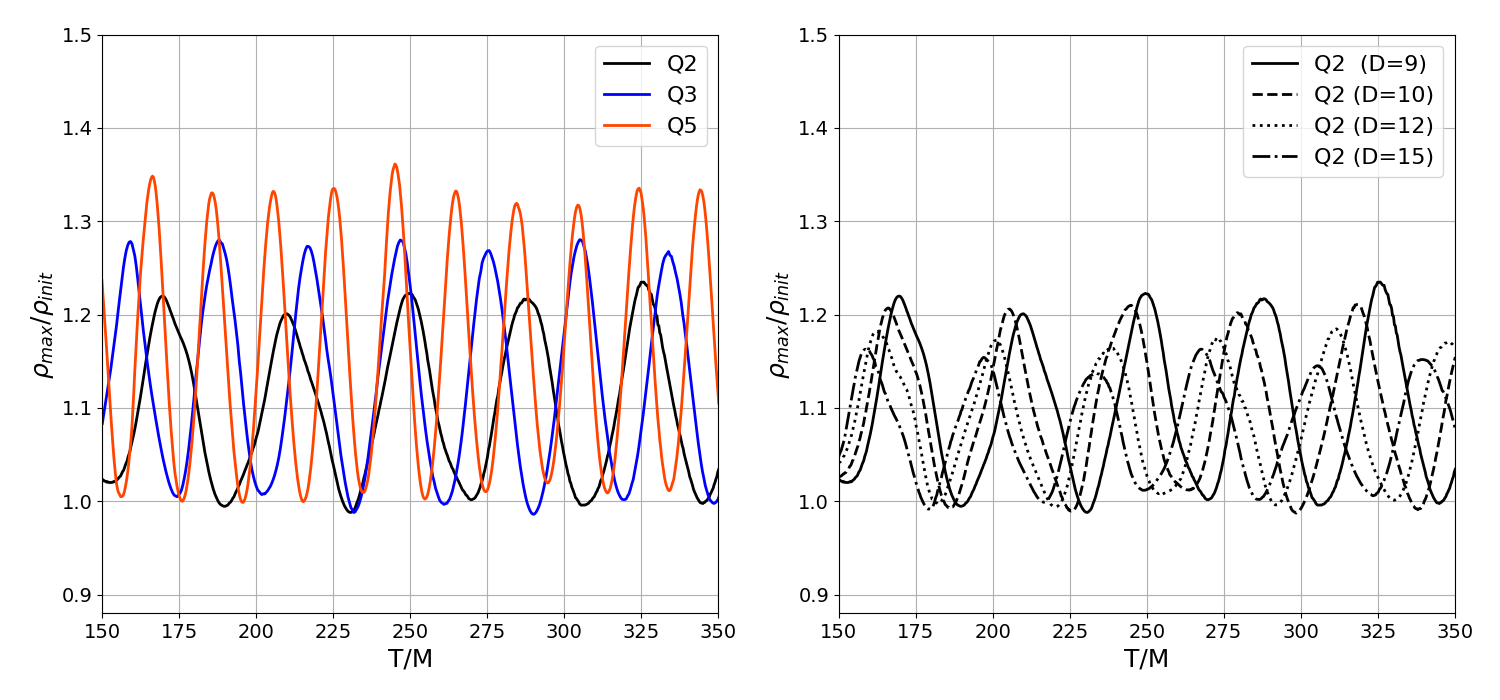
Figure 3: Oscillations in the normalized central density of the NS. Here, $\rho_{max}$ is the central density of the neutron star at any time $t$ and $\rho_{init}$ is the central density at initial time. Panel on the left shows a comparison of density oscillations for different mass ratio while panel on the right shows the comparison for four different separation for mass ratio 2.

4 Results

4.1 Inspiral and Merger Dynamics

During the late inspiral stage of a BHNS binary, the NS will face a constant battle between the tidal forces from the BH and its self gravity. Depending on the mass of the BH, this could lead to the complete disruption of the star before it gets swallowed by the BH. The tidal forces by the NS could also inflict deformations in a companion, such as in a double NS binary merger. However, although not generally accepted [56], there is strong evidence that BHs are immune to tidal deformations [57]. Thus, there are potentially fundamental differences between a BBH and a BHNS.

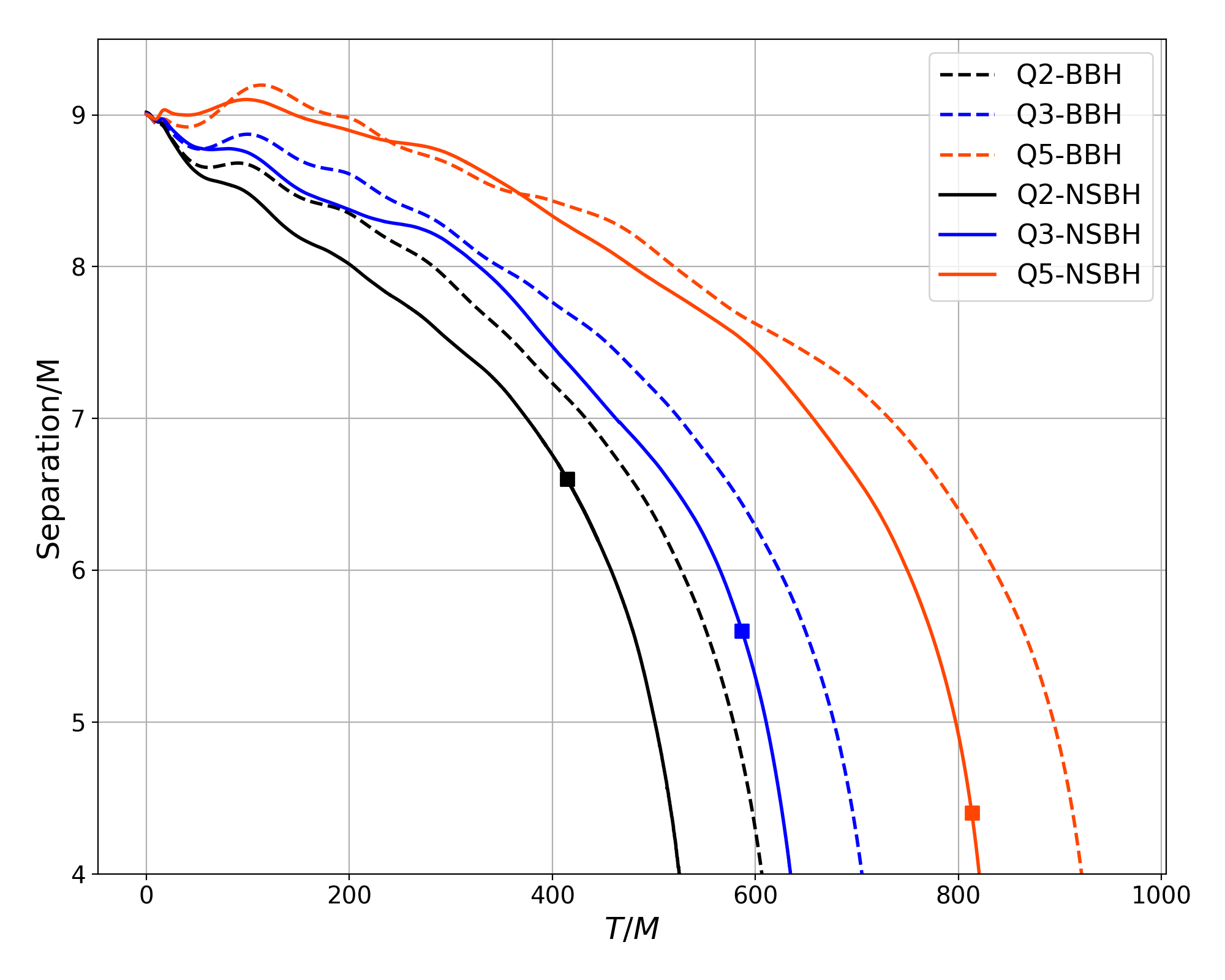
Figure 4: Evolution of the binary coordinate separation for each BHNS and BBH binary described in Table 1. Solid squares denote when the binary has reached the tidal radius as computed by Eq. 36.

For compact object binaries, the luminosity of gravitational radiation and the rate of change of radiated angular momenta depend on the mass ratio as $q^{2}/(1+q)^{4}$ [32]. As a consequence, the higher the mass ratio, the longer it takes for the binary to merge. In Figure 4, we show the evolution of the coordinate separation of the binary for each of the BHNS systems described in Table 1 and its BBH counterpart. The delay as a function of $q$ for both, the BHNS binaries and BBHs, is evident in this figure. For a given $q$, we also see that the coordinate separation of the BHNS binary decreases faster than its corresponding BBH. For the $q=5$ case, the BBH and BHNS follow each other up to a separation $\sim 7.5\,M$. For $q=3$, the binaries diverge a little earlier at a separation of approximately $8\,M$. The earliest deviation occurs for the $q=2$ case, approximately at a time $50\,M$ from the start of the simulation. That is, as the mass ratio increases, the BHNS binaries resemble longer a BBH. The difference in the binary separation between BBH and BHNS systems grows stronger as the merger is approached.

Regarding the time when compact objects merge, for BBH, it is marked by the sudden formation of a common apparent horizon. The apparent horizon appears a few $M$s before the gravitational radiation reaches peak luminosity. For BHNS binaries, we do not have the formation of a common apparent horizon since the only horizon is the one from the single BH in the binary. Therefore, when making comparisons near coalescence, we will focus on the time when the gravitational radiation reaches peak luminosity (corresponding to the peak of $|\Psi_{4}|$).

In Table 2, $T_{mx}$ denotes the retarded time to peak luminosity and $\Delta_{mx}$ the final BH offset at $T_{mx}$. Notice that the BHNS binaries reach peak luminosity earlier than their corresponding BBH. We will address the reasons for this difference when we discuss the GWs emitted by the binaries. An interesting aspect to point out is that this difference does not decrease monotonically with $q$.

Also in Figure 4, denoted with solid squares is the coordinate separation when the binary reaches the tidal radius as estimated by [32, Eq.17.19]

$$\frac{R_{T}}{M_{h}}\simeq 2.4\,q^{-2/3}\,C^{-1}\,.$$ (34)

Relative to the ISCO radius $R_{I}\simeq 6\,M_{h}$, the tidal radius is given by

$$\frac{R_{T}}{R_{I}}\simeq\left(\frac{q}{4.3}\right)^{-2/3}\left(\frac{C}{0.15}\right)^{-1}\,.$$ (35)

For $q\geq 4.3$, $R_{T}\leq R_{I}$, and the NS is swallowed by the BH relatively intact. For reference, the tidal radius in units of the total mass $M$ is given by

$$\frac{R_{T}}{M}\simeq 16\,\frac{q^{1/3}}{1+q}\left(\frac{C}{0.15}\right)^{-1}\,.$$ (36)

Thus, $R_{T}/M\simeq 6.6,\,5.6$ and $4.4$ for $q=2,\,3$ and $5$, respectively. For reference, the coordinate separation at the beginning of the simulations is $9\,M$

System	$q$	$E_{ADM}/M$	$J_{ADM}/M^{2}$	$e/10^{-3}$	$T_{mx}/M$	$\Delta_{mx}/M$
BBH	2	0.9901	0.829	6.3	648	0.027
BHNS	2	0.9914	0.829	6.8	537	0.746
BBH	3	0.9918	0.702	5.5	743	0.058
BHNS	3	0.9921	0.702	8.3	662	0.782
BBH	5	0.9939	0.523	10.5	957	0.037
BHNS	5	0.9941	0.523	9	848	1.03

Table 2: Binary system, mass ratio $q$, ADM energy $E_{ADM}$ and angular momentum $J_{ADM}$, eccentricity $e$, retarded time to peak luminosity $T_{mx}$, and final BH offset $\Delta_{mx}$ at $T_{mx}$.

To get an overall sense of the inspiral and merger, Figures 5, 6 and 7 show snapshots of the rest mass density in the orbital plane for all the cases under consideration. For $q=2$, the tidal forces from the BH trigger mass shedding early on, at approximately $440\,M$ from the beginning of the simulation when the binary separation is approximately $6.25\,M$. This happens roughly $96\,M$ before the peak luminosity. Figure 5 shows four evolution snapshots for this case. The BH is represented by a black circle with white boundary. The initial central density of star is $0.02\,M^{-2}$ ($7.7\times 10^{14}~{}\textrm{g/cm}^{3}$). Top left panel shows a snapshot at time $96\,M$ before the peak luminosity, when the NS begins to be disrupted. Top right panel shows the stellar disruption at the time of merger. Notice that the NS has been completely destroyed, deforming into a spiral arm around the BH which extends to $7\,M$ beyond the hole. Bottom left panel show the circularization stage of matter around the BH about 100 M after the merger. We found that about $90\%$ of the star’s material falls into the BH within the first $100\,M$ of evolution while the remaining material continues to expand outwards slowly morphing into an accretion disk. The bottom right panel shows the final state of the accretion disk 500 M after the merger, reaching a core density of $\sim 10^{-4}\,M^{-2}$ ($\sim 10^{12}\,\textrm{g/cm}^{3}$).

The $q=3$ BHNS merger follows the $q=2$ steps but not as dramatic in terms of disruption effects. In Figure 6, the top left panel shows the beginning of tidal disruption and tail formation $78\,M$ before the merger. The channel of mass transfer is much narrower due to weaker tidal interactions. This is followed by complete disruption of the star at the merger shown in the top right panel more than $95\%$ of which is consumed by the BH within $30\,M$ . The bottom left panel shows matter circularization $30\,M$ after the merger. The bottom right panel depicts the formation of a very tenuous accretion disk $500\,M$ after peak emission with characteristic density of $\sim 10^{-5}\,M^{-2}$ ($\sim 10^{11}\,\textrm{g/cm}^{3}$).

As mentioned before, the $q=5$ for a BHNS behaves more like a BBH, with the star remaining almost intact by the time it reaches $R_{I}$ since $R_{T}\simeq 4.4\,M$. The top left panel in Figure 7 shows a snapshot at $45\,M$ prior to the merger. There are hints of material being stripped from outer layers of the star. The top right panel shows the situation $20\,M$ before the merger and the bottom left panel at the merger. The bottom right panel shows the result $20\,M$ after the merger. At that point, $99\%$ of the NS has been swallowed by the hole. This leaves a remnant state with extremely low densities. Since there is very little change in this case of triggering electromagnetic signatures, the BHNS and BBH are almost indistinguishable from each other. This will be more apparent when we compare GW emissions.

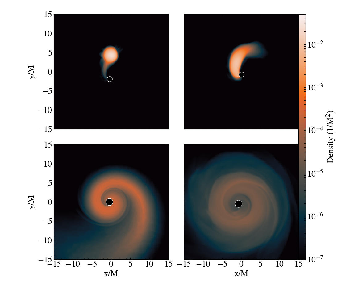
Figure 5: Snapshots of the rest mass density for the $q=2$ BHNS. The BH is represented by a black circle with white boundary. Panel on the top left shows the beginning of stellar disruption $96\,M$ before peak luminosity. Top right panel shows the stellar disruption at the time of merger followed by circularization of matter forming an spiral arm around BH $100\,$M after the merger (bottom left panel). The last panel shows the final state of the accretion disk 500 M after the merger.

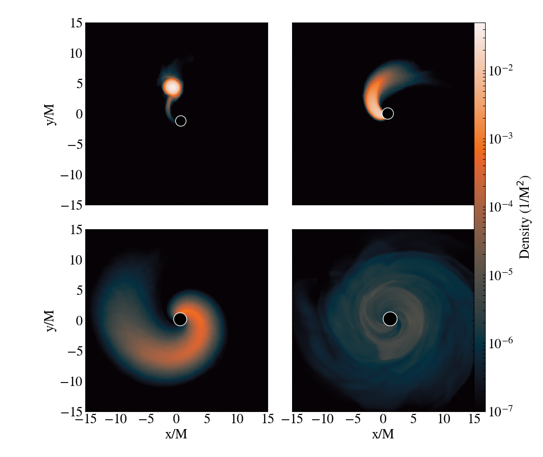
Figure 6: Snapshots for $q=3$ BHNS merger. Top left panel shows the beginning of tidal disruption and tail formation $78\,M$ before peak luminosity, and the top right panel shows the consumption of disrupted star by the BH at peak luminosity. The bottom left panel shows matter circularization $30\,M$ after peak luminosity. The bottom right panel depicts the formation of a very tenuous accretion disk $500\,M$ after peak emission.

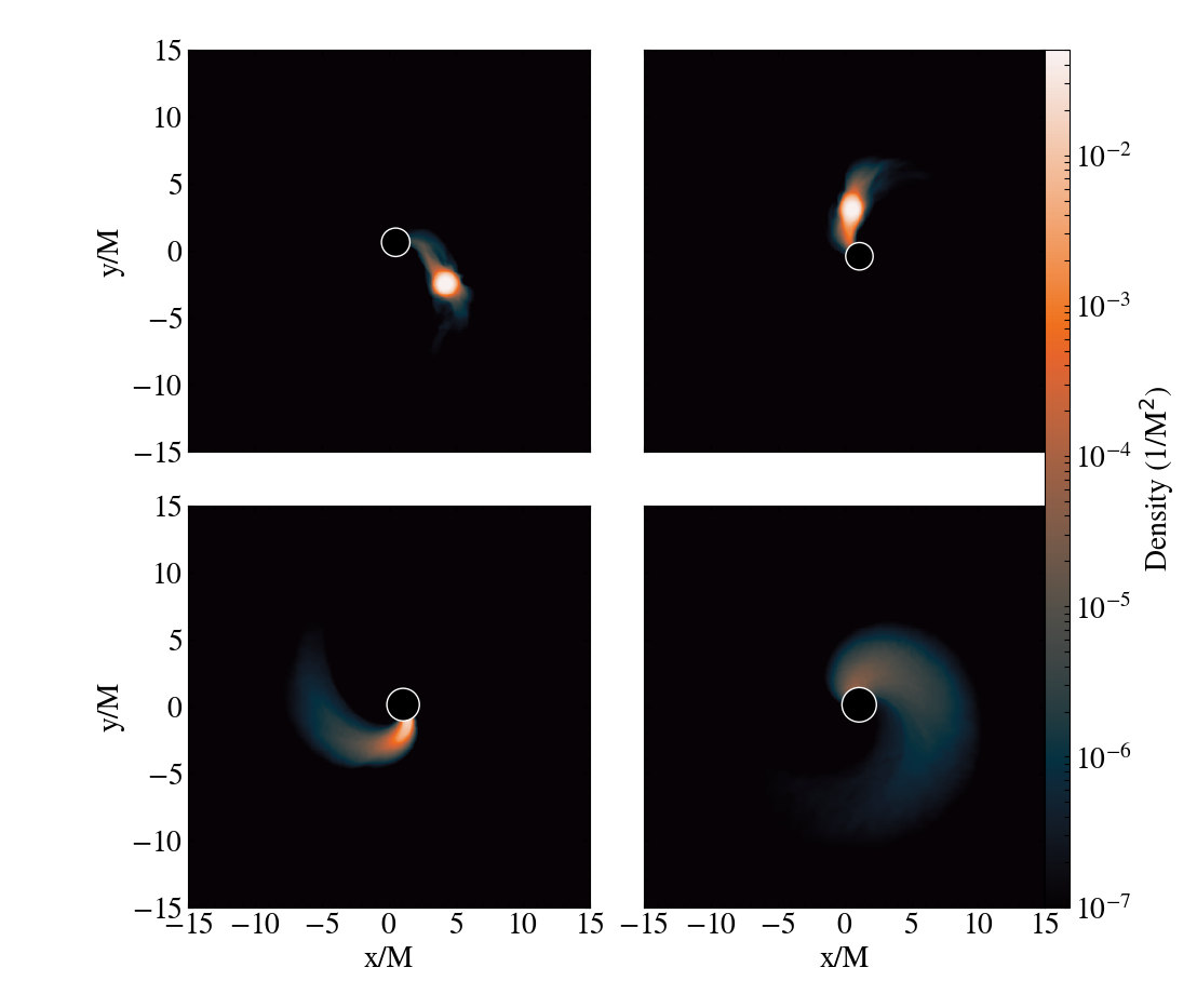
Figure 7: Snapshots for the BHNS $q=5$ binary merger. The top left panel shows the rest mass density at $45\,M$ prior peak luminosity. The top right panel shows the situation $20\,M$ before peak luminosity and the bottom left panel at the merger. The bottom right panel shows the result $20\,M$ after peak luminosity.

System	$q$	$M_{h}/M$	$M_{*}/M$	$M_{f}/M$	$M_{c}/M$	$M_{td}/M$	$a_{f}$	$E_{rad}/M$	$v_{k}(\textrm{km/s})$
BBH	2	0.667	0.333	0.9073	0.9598		0.617	0.0295	147.7
BHNS	2	0.667	0.333	0.8984	0.9659	0.019	0.683	0.0077	39.1
BBH	3	0.750	0.250	0.9319	0.9712		0.5405	0.0208	169
BHNS	3	0.750	0.250	0.9308	0.974	0.008	0.563	0.0102	29.2
BBH	5	0.833	0.167	0.9598	0.9823		0.4166	0.0118	135.7
BHNS	5	0.833	0.167	0.9603	0.9834	0.0004	0.4203	0.0106	103.5

Table 3: $M_{h}$ irreducible mass of the initial BH (mass of the larger BH in BBH cases), $M_{*}$ initial mass of the NS (irreducible mass of the smaller BH in BBH cases), $M_{f}$ irreducible mass of the final BH, $M_{c}$ Christodoulou mass of the final BH, $M_{td}$ mass left outside the final BH, $a_{f}$ dimensionless spin of the final BH, $E_{rad}$ radiated energy, and $v_{k}$ its kick.

4.2 The Final BH

The mass and spin of the final BH in a BHNS merger will depend on the extent to which the NS is devoured by the BH. Table 3 shows $M_{h}$ the irreducible mass of the initial BH (mass of the larger BH in BBH cases), $M_{*}$ the initial mass of the NS (irreducible mass of the smaller BH in BBH cases), $M_{f}$ the irreducible mass of the final BH, $M_{c}$ the Christodoulou mass of the final BH, $M_{td}$ the mass left outside the final BH, $a_{f}$ the dimensionless spin of the final BH, $E_{rad}$ the radiated energy, and $v_{k}$ the kick of the final BH.

First thing to notice is that the irreducible and Christodoulou masses of the final BH in the BHNS and BBH are comparable. On the other hand, the energy radiated and the spins and kicks of the final BH differ significantly. BHNS mergers produce a final hole with higher spin but with a lower kick. The differences in both the final spin and kick decrease as $q$ increases since the binary becomes more BBH-like. The main culprits of the differences are again the tidal deformations and disruption of the NS.

To understand the differences in the mass, spin and kicks of the final BH, we plot in Figure 8 their evolution. The top left panel shows with solid lines the growth of the irreducible mass of the BH in BHNS mergers. Dashed horizontal lines denote the final mass of BH, $M_{f}$, for the corresponding BBH merger. $T=0$ is the time at the peak luminosity. Notice that as expected, for $q=5$, the growth is abrupt because the NS is swallowed almost intact, thus mimicking a BBH in which a common apparent horizon suddenly appears to signal the merger. For $q=2$ the transitions takes much longer and the final mass of the BH does not get closer to the mass of the BBH final BH. This is because of the material left behind. The rates at which the mass of the final BH changes are depicted in the top right panel of Figure 8. The rates clearly emphasize that the growth is sharp for $q=5$ and smoother for $q=2$.

Regarding the spin of the final BH, the middle left panel in Figure 8 shows with solid lines the growth of the spin of the final BH for BHNS binaries given by $S_{z}/M^{2}$, and, for reference, dashed horizontal lines denote the spin of the final BH for the corresponding BBH merger. Middle right panel shows the corresponding spin growth rate $\dot{S}_{z}/M$. Here also one observes that for lower $q$ the transition is smoother. Important to notice that $S_{z}/M^{2}$ is not the dimensionless spin of the final BH. The dimensionless spin is given $a_{f}=S_{z}/M_{c}^{2}$ with $M_{c}$ the Christodoulou mass of the final BH. The reason why $a_{f}$ for BHNS are higher is because, as we will see later, the emission of gravitational radiation carrying out angular momentum is lower; thus, at merger, the final BH is left with high angular momentum.

For the kicks of the final BH the situation reverses. The gravitational recoil is lower for BHNS mergers. This is because most of the accumulation of the gravitational recoil in compact object binaries takes place in the last few orbits, but this is precisely the stage when BBH and BHNS differ the most. As the NS undergoes disruption, and thus lose its compactness, the BHNS binary radiates less and with it the opportunity to carry out linear momentum. This is clear from the bottom panels in Fig. 8 where the left panel shows the accumulation of linear momentum emitted by GWs for both, the BHNS (solid lines) and BBH systems (dashed lines). It is interesting to notice that while the magnitude of the kicks for BBHs are $Q5<Q2<Q3$, consistent with the results in Ref. [58], the kicks for BHNS systems are $Q3<Q2<Q5$.

Figure 8: Top left panel shows with solid lines the growth of the irreducible mass of the BH as a function of time for BHNS binaries. Dashed horizontal lines denote the final mass of BH for the corresponding BBH merger. $T=0$ is the time at peak luminosity. Top right panel shows the corresponding mass growth rate $\dot{M}_{h}$. Middle left panel shows with solid lines the growth of the spin of the BH for BHNS binaries. For reference, dashed horizontal lines denote the spin of the final BH for the corresponding BBH merger. Middle right panel shows the corresponding spin growth rate $\dot{S}_{z}$. Bottom left panel shows the accumulation of linear momentum emitted by GWs for both, the BHNS (solid lines) and BBH systems (dashed lines). Bottom right panel depicts the corresponding rate of linear momentum accumulation.

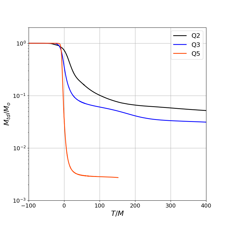
Figure 9: Rest mass of the tidal debris $M_{td}$ outside the horizon normalized to the initial rest mass of the NS.

4.3 Tidal Debris

We have seen from Figure 5 that the disruption of the NS would leave behind a trail of material in the vicinity of the BH. To get a better understanding of how the remnant material outside the BH depends on the mass ratio $q$, we plot in Figure 9 the rest mass of tidal debris $M_{td}$ outside the BH normalized to the initial rest mass of the NS. After peak luminosity, $M_{td}$ accounts for both the mass in the accretion disk and the unbound debris. For $t<-50\,M$, the material from the NS has not reached yet the hole; thus, $M_{td}$ includes the entire mass of the star.

For $q=2$, approximately $90\%$ of the mass of the NS falls into the BH within $t\sim 100\,M$ after peak luminosity. By $t\sim 400\,M$, the accretion process slows down, leaving behind $~{}5$% of the mass of the NS. The $q=3$ case follows a similar trend. At $t\sim 100\,M$, the BH has already consumed $\sim 94\%$ of the stellar material, and at $t\sim 400\,M$ only $\sim 3\%$ is left outside the holes. As expected, the case $q=5$ is significantly different since $99\%$ of star is devoured by the hole just $t\sim 20\,M$ after peak luminosity, leaving outside barely any material. Table 3 lists the final $M_{td}$ for each case. Comparing with the results in [7] and [14], we find that our masses agree well for $q=2$ but they differ by approximately $20\%$ for $q=3$. A possible explanation for this difference could be the effects from the artificial atmosphere used in this type of simulations to handle the vacuum regions in the computational domain.

4.4 Gravitational Waves

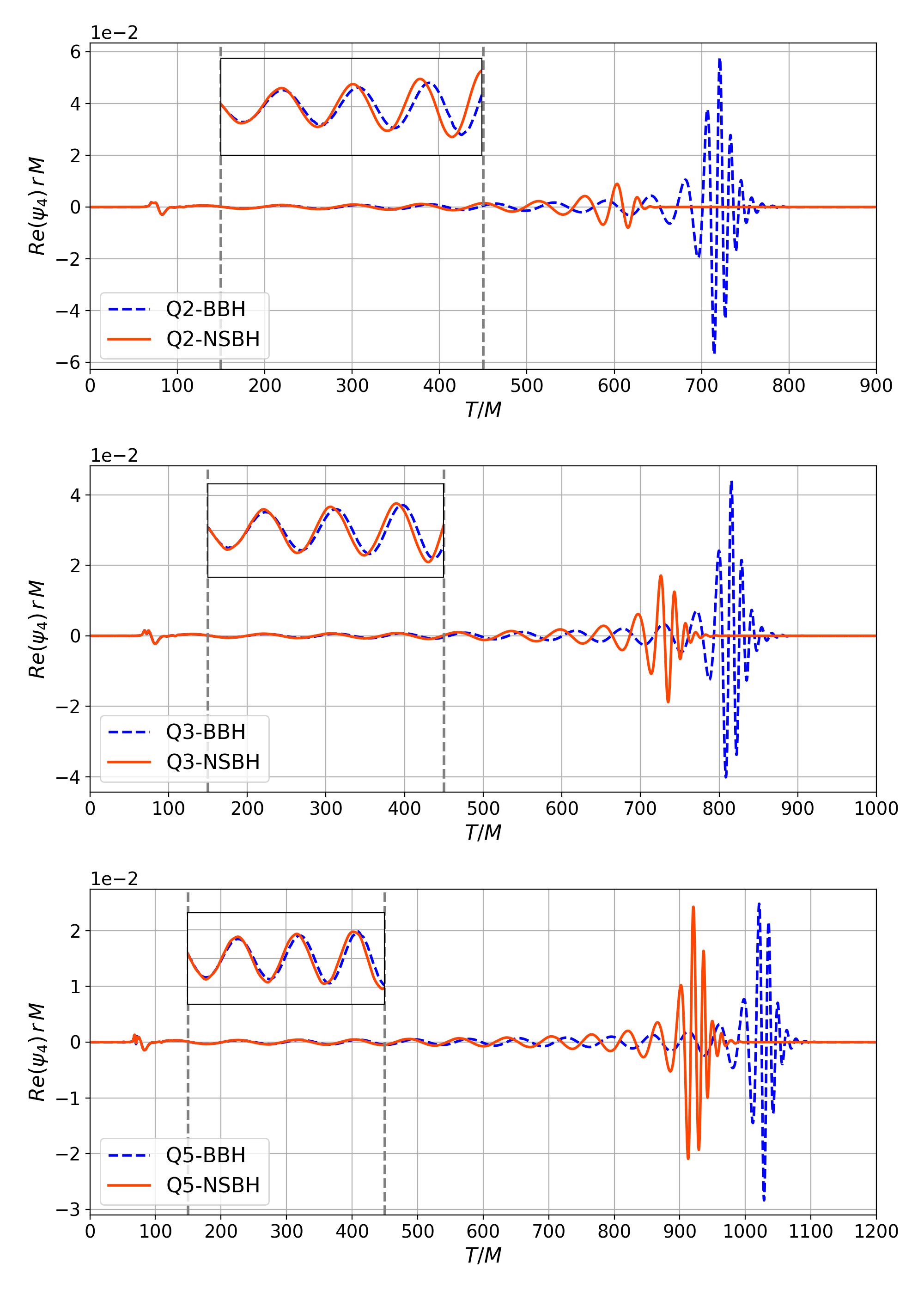
Figure 10: Real part of the (2,2) mode of the Weyl scalar $\Psi_{4}$. From top to bottom $q=2,\,3$ and 5. BHNS waveforms are depicted with solid lines and the corresponding BBH waveform with dashed lines. The inset shows the waveforms early on between $150\leq T/M\leq 450$.

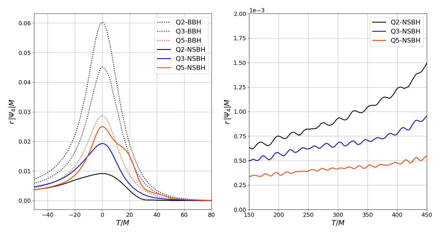
Figure 11: Amplitude of the (2,2) mode of $\Psi_{4}$. The left panel shows the waveform amplitudes of both the BBH and BHNS mergers around peak luminosity. The right panel shows the waveform amplitudes for BHNS binaries during the time window of the insets in Figures 10.

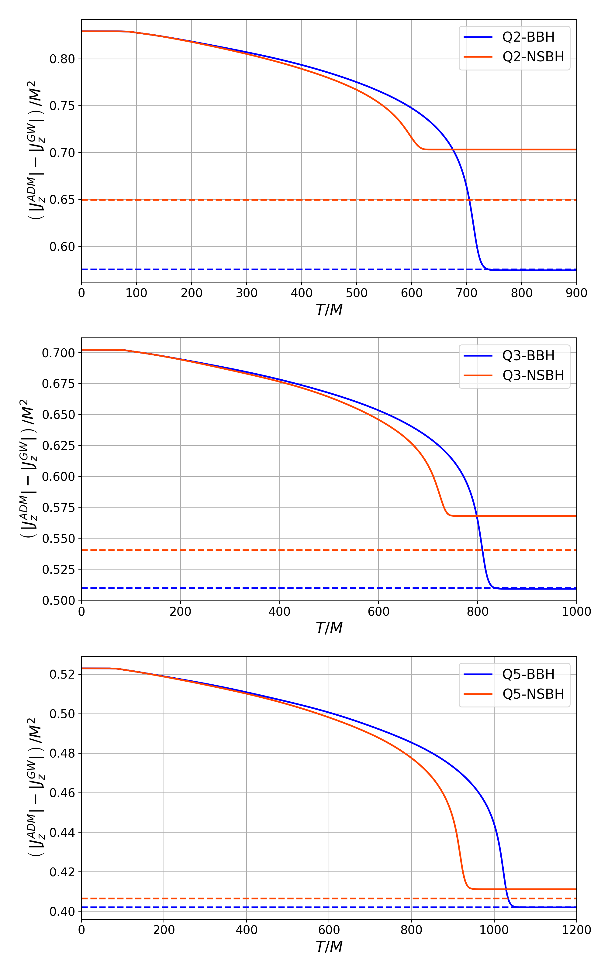
Figure 12: $|J_{z}^{ADM}|-|J_{z}^{GW}|$ with $J_{z}^{ADM}$ is the ADM angular momentum in the initial data and $J_{z}^{GW}$ the angular momentum carried out by GWs. Dashed lines denote the angular momentum of the final BH. For both, dashed and solid lines, blue denotes the BBH case and red the BHNS. From top to bottom the cases $q=2$, 3 and 5, respectively.

Figure 10 shows the real part of the (2,2) mode of the Weyl scalar $\Psi_{4}$ for the BHNS binaries (solid line) together with their corresponding waveform for the BBH (dashed line). The insets show the waveforms early on between $150\leq T/M\leq 450$, from which one can see that the BBH and BHNS waveforms are closer to each other as $q$ grows. In this figure, it is also evident that $\Psi_{4}$ for BHNS binaries reaches its maximum amplitude earlier. Since peak luminosity also signals that the binary merges around that time, this also implies that BHNS binaries merge earlier than their corresponding BBH system. Before addressing the reasons for the prompt merger of BHNS binaries, we will discuss the differences in the peak luminosity.

Figure 11 depicts the amplitude of $\Psi_{4}$. The left panel shows the waveform amplitudes of both the BBH and BHNS mergers around peak luminosity. For the BBH amplitudes, from highest to lowest are $q=2,\,3$ and 5, respectively. This is not surprising since, as stated before, the luminosity of gravitational radiation depends on the mass ratio as $q^{2}/(1+q)^{4}$. Interestingly, the situation reverses for BHNS systems. The amplitudes are not only lower than those of the BBHs, but now instead from highest to lowest are $q=5,\,3$ and 2. For $q=2$ and 3, the decrease in amplitude is due to the disruption the NS experiences that makes it loose compactness and thus decrease the quadrupole moment of the binary. The $q=5$ BHNS case is comparable to the BBH case because, once again, this is the case in which the star merges with the hole without significant disruption. The “bump” observed in this case is an artifact of the way the spherical decomposition is done. It assumes that the coordinate system is centered at the origin of the computational domain. From Table 2, we see that at merger time the center of mass of the binary for $q=5$ is already displaced $1\,M$ from the origin. As a consequence the (2,2) mode has contributions from higher modes. The other two $q$ cases also undergo displacements, but they are not as large, and the higher modes for low $q$’s are not as dominant as in $q=5$.

The right panel in Figure 11 shows the amplitudes of $\Psi_{4}$ for BHNS binaries during the time window of the insets in Figure 10. Since this is during the early stage of the simulation, disruption effects do not play a significant role yet, and the situation resembles the BBH case in which the amplitude decreases with $q$. The oscillations in the amplitude of $\Psi_{4}$ are due to the spurious oscillations in the NS because of the initial data. In separating amplitude and phase in $\Psi_{4}$, we did not explicitly separated the effects from the NS oscillations, thus, the oscillatory behavior remains in the amplitude.

Regarding the prompt merger of BHNS systems, there are only two channels to transport angular momentum out of the binary to harden it. As with BBH systems, one channel is via GW emission. The other channel is transport of angular momentum by the tidal debris. Because the initial data is constructed using a generalization of the puncture Bowen-York approach, the ADM angular momentum in the initial data is the same for the BHNS binary and its corresponding BBH as stated in Table 2. Since we are dealing with non-spinning BHs and NSs, we only need to look at the angular momentum perpendicular to the orbital plane, namely the $z$-component. In Figure 12, we plot with solid lines $|J_{z}^{ADM}|-|J_{z}^{GW}|$ from top to bottom the cases $q=2$, 3 and 5, respectively. Here, $J_{z}^{ADM}$ is the ADM angular momentum in the initial data, and $J_{z}^{GW}$ is the angular momentum carried out by GWs. In Figure 12, dashed lines denote the angular momentum of the final BH. For both, dashed and solid lines, blue denotes the BBH case and red the BHNS. Since for BBHs there is only one channel, GWs, to remove angular momentum from the binary, $|J_{z}^{ADM}|-|J_{z}^{GW}|$ after merger and ring-down closely matches the value of the angular momentum of the final BH. The slight difference is because of the junk radiation in the initial data.

The situation is different for BHNS binaries. The first thing to notice in Figure 12 is that there is a gap between the value that $|J_{z}^{ADM}|-|J_{z}^{GW}|$ reaches after merger and ring-down and the value of the angular momentum of the final BH. This gap is closed if in addition one includes the angular momentum carried out by the tidal debris. The gap is larger the lower the $q$ because the tidal disruptions is stronger. The other feature in Figure 12 is that the decrease of $|J_{z}^{ADM}|-|J_{z}^{GW}|$ is faster for BHNS binaries. The differences start appearing after approximately $300\,M$, $400\,M$ and $500\,M$ of evolution for $q=2$, 3 and 5, respectively. At those times, as clear from equation 36, the binary is far from the tidal disruption separation. Therefore, the most likely culprit is the tidal deformations on the NS. This effect was pointed out in Ref. [28] using post-Newtonian arguments. Specifically, it was noted that the deformation in the NS introduces a correction term in the potential whose magnitude increases steeply with the decrease of the orbital separation. The effect is an acceleration of the inspiral and thus on the emission of GWs, leading to a prompt merger.

4.5 Quasi-normal Ringing

Next is to discuss the onset of the quasi-normal ringing of the final BH. Given the mass and the spin of the final BH in Table 3, we compute from the standard fits in the literature [59] the quasi-normal frequency and decay time for the (2,1), (2,2) and (3,3) modes. The values are given in Table 4. Figure 13 shows the amplitude (left panels) and phase (right panels) of the (2,1), (2,2) and (3,3) modes of $\Psi_{4}$ after peak luminosity when the final BH is expected to undergo quasi-normal ringing. In these log-linear for the amplitude and linear-linear for the phase plots, quasi-normal ringing (i.e. exponentially damped sinusoidal) would show up as linear dependence with time for both the amplitude and the phase. For reference, the solid lines are the quasi-normal ringing computed from Table 4.

For the (2,1) mode, we see that the only case showing quasi-normal behaviour is the $q=5$, the one with the more BBH-like characteristics. For the other two cases, there are two factors that prevent a clean quasi-normal ringing. One is that the geometry of the tidal debris does not favor excitation of the final BH in this mode. The other is that, during the time spanned in the figure for the decay of $\Psi_{4}$ ($\sim 100\,M$), the final BH is still growing as one can see from Figure 8. The (2,2) mode is the one with more noticeable quasi-normal characteristics, in particular in the phase. The exponential decay of the amplitude is cleaner for the $q=3$ case, and the $q=5$ case shows the bumps associated with the contributions from higher modes due to the center of mass displacement. The $q=2$ case shows exponential decay after $50\,M$, which according to the left panel in Figure 8 is when the BH has almost stopped accreting the debris from the disrupted NS. Interestingly, in all cases, the phase of the (3,3) mode shows an approximate linear growth (i.e. constant frequency of oscillation), but only in the case $q=5$ the growth matches that of quasi-normal ringing. Similarly, exponential decay in the amplitude is not as clear with the exception of the $q=5$. The oscillations in the $q=3$ we conjecture are associated with the accretion of tail of debris observed in the bottom left panel in Figure 6.

System	$q$	$\omega_{f}^{2,1}$	$\tau_{f}^{2,1}$	$\omega_{f}^{2,2}$	$\tau_{f}^{2,2}$	$\omega_{f}^{3,3}$	$\tau_{f}^{3,3}$
BHNS	2	0.471	11.73	0.546	11.8	0.866	11.49
BHNS	3	0.446	11.42	0.499	11.42	0.794	11.06
BHNS	5	0.421	11.26	0.454	11.27	0.726	10.86

Table 4: Quasi-normal frequencies and damping times computed from the mass and the spin of the final BH in Table 3 using the standard fits in the literature [59].

System	$q$	$\omega^{2,1}$	$\tau^{2,1}$	$\omega^{2,2}$	$\tau^{2,2}$	$\omega^{3,3}$	$\tau^{3,3}$
BHNS	2	0.155	55.62	0.543	9.898	0.603	9.86
BHNS	3	-0.332	13.1	0.492	11.32	0.483	11.52
BHNS	5	0.436	10.83	0.449	11.08	0.71	10.08

Table 5: Quasi-normal frequencies and damping times computed from fitting the data in Figure 13.

Figure 13: Amplitude (left panels) and phase (right panels) of $\Psi_{4}$ after peak luminosity for BHNS systems. The solid lines are the quasi-normal ringing computed from Table 4.

Figure 14: Panels on the left show the real part of the (2,2) mode of the strain. From top to bottom $q=2,\,3$ and 5. BHNS waveforms are depicted with solid lines and the corresponding BBH waveform with dashed lines. Panels on the right show the phase differences between BBH and BHNS waveforms.

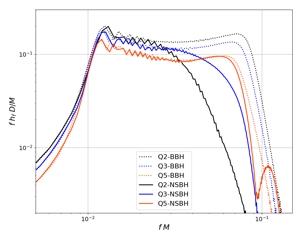
Figure 15: Fourier Spectrum of the Strain

4.6 Spectrum and Mismatches

Ultimately, comparisons between BBH and BHNS systems would be incomplete if not looked through the eyepiece of data analysis tools. The focus of a follow up paper will pay particular attention to observational signatures from the compactness of the NS. For the present work, we start by showing in Figure 14 the strain of both the BHNS and BBH systems for each mass ratio (from top to bottom). Panels on left show the plus polarization of the $(2,2)$ mode of the strain and panels on the right show the phase difference between the BHNS and BBH waveforms. We observe very similar characteristics to $\Psi_{4}$ as seen in Figure 10. The peak of strain in the BHNS systems occurs earlier than the BBH for the same mass ratio suggesting early mergers. The two signals overlap for longer durations with increasing mass ratio as seen from the phase differences. The phase differences grow steadily reaching a peak beyond which the BHNS signal dies off as the system reaches a stable state.

Figure 15 shows the Fourier spectrum of strain of both the BHNS and BBH systems. It is evident how the BHNS and the corresponding BBH system agree early on for low frequencies, with the $q=5$ following each other through merger.

Next we show in Table 6 mismatches, $1-\mathcal{O}(h_{1},h_{2})$, relative to LIGO and the Einstein Telescope, with the matches given by

$$\mathcal{O}(h_{1},h_{2})=\frac{\max_{\phi_{c},t_{c}}\langle h_{1},h_{2}\rangle}{\sqrt{\langle h_{1},h_{1}\rangle\langle h_{2},h_{2}\rangle}}$$ (37)

maximized by the time and phase at coalescence, $t_{c}$, and $\phi_{c}$. The inner product $\langle\;,\;\rangle$ is defined as

$$\langle h_{1},h_{2}\rangle\equiv 4Re\int_{0}^{\infty}\frac{\tilde{h}^{*}_{1}(f)\tilde{h}_{2}(f)}{S_{n}(f)}df$$ (38)

In this expression, $h$ are strains including modes up to $l=8$ and $S_{n}(f)$ is the one sided power spectral density of the detector noise. The mismatches in Table 6 include three different inclinations: $i=0,\,\pi/6$ and $\pi/3$. As expected, for $i=0$ (face-on), the mismatch is highest for $q=2$ because the (2,2) mode dominates in this case; the mismatch decreases with increasing mass ratios consistent with our previous observations. Across the detectors, mismatches are smaller for the Einstein Telescope compared to LIGO, given the higher sensitivity of the former. For $i=\pi/6$, the trend remains similar though the mismatch values decrease for $q=2$ while increase for other two cases because of the contributions from higher modes. This situation becomes more visible for $i=\pi/3$, where the contributions of higher modes increase significantly. The mismatch now increases with mass ratio with $~{}12\%$ mismatch between BBH and NSBH waveforms for $q=5$ and $~{}10\%$ mismatch for $q=3$. This shows the importance of higher modes in the study of mixed binaries at high mass ratios.

$q$	Detector	$i=0$	$i=\pi/6$	$i=\pi/3$
2	LIGO	0.0845	0.0756	0.074
2	ET	0.0767	0.0686	0.0666
3	LIGO	0.0611	0.0731	0.0984
3	ET	0.0464	0.0576	0.0814
5	LIGO	0.0046	0.0401	0.1194
5	ET	0.0030	0.0349	0.1072

Table 6: Mismatches between BBH and BHNS waveforms for three different inclination angle $i$ and for the Einstein Telescope (ET) and LIGO.

5 Conclusions

For high mass ratio systems, distinguishing BHNS binaries from BBH binaries will incur challenges because the NS is swallowed by the hole without experiencing significant disruption. To investigate the transition of the merger behaviour of a BHNS into a BBH-like system, we have carried out three BHNS merger simulations and their corresponding BBH mergers for mass ratios $q=2,\,3$ and $5$. The BHNS system with $q=2$ represents the case of total NS disruption before merger, and the $q=5$ case is an example of a BBH-like merger. The focus was on the effects that the disruption of the NS imprints on the inspiral and merger dynamics, the properties of the final BH, the accretion disk, the GWs, and the strain spectrum and mismatches. A secondary objective of the study was to demonstrate the effectiveness of the method we developed in Ref. [30] to construct initial data with a generalization of the Bowen-York data for BH punctures to the case of NSs.

The most noticeable feature observed in the simulations of the merger dynamics of the BHNS binaries was that they merge earlier than their corresponding BBHs. We found that the dominant factor hardening the mixed binary is the enhanced angular momentum emission carried out by the GWs due to the tidal deformations in the NS. On the other hand, the tidal disruption of the NS suppresses the gravitational recoil of the final BH in BHNS mergers when compared with BBHs. Regarding the final BH, its mass is comparable between the BHNS and BBH systems. This, however, is not the case regarding the final spin. For instance, in the case of $q=2$, the tidal debris as is accreted by the hole increases the spin by approximately $10\,\%$. The same tidal debris has an influence in the quasi-normal ringing of the final BH. For low $q$’s only the (2,2) mode exhibits a clean damped exponential sinusoidal behavior. In terms of mismatches, the most favorable configuration to distinguish between BHNS and BBH systems with large $q$’s would be that for large inclinations where higher modes are more influential.

Acknowledgements

This work is supported by NSF grants PHY-1908042, PHY-1806580, PHY-1550461. MGL acknowledges the support from the Mexican National Council of Science and Technology (CONACyT) CVU 391996. We would also like to acknowledge XSEDE (TG-PHY120016) and the Partnership for an Advanced Computing Environment (PACE) at the Georgia Institute of Technology, Atlanta, Georgia, USA for providing necessary computer resources for this study. We thank Chris Evans, Deborah Ferguson, Zachariah Etienne and Deirdre Shoemaker for discussions and sharing their resources for this work. We would also like to thank the reviewers for extremely useful feedback and comments. Finally, the authors would also like to express their gratitude to all the front-line workers for their efforts and dedication to keep us all safe during these challenging times.

References

- [1] Abbott R et al. (LIGO Scientific, Virgo) 2020 (Preprint 2010.14527)
- [2] Abbott B et al. (LIGO Scientific, Virgo) 2017 Phys. Rev. Lett. 119 161101 (Preprint 1710.05832)
- [3] Abbott B et al. (LIGO Scientific, Virgo) 2020 Astrophys. J. Lett. 892 L3 (Preprint 2001.01761)
- [4] Abbott R et al. (LIGO Scientific, Virgo) 2020 Astrophys. J. Lett. 896 L44 (Preprint 2006.12611)
- [5] Hayashi K, Kawaguchi K, Kiuchi K, Kyutoku K and Shibata M 2020 (Preprint 2010.02563)
- [6] Foucart F, Duez M, Kidder L, Nissanke S, Pfeiffer H and Scheel M 2019 Phys. Rev. D 99 103025 (Preprint 1903.09166)
- [7] Shibata M, Kyutoku K, Yamamoto T and Taniguchi K 2009 Phys. Rev. D 79 044030 [Erratum: Phys.Rev.D 85, 127502 (2012)] (Preprint 0902.0416)
- [8] Etienne Z B, Faber J A, Liu Y T, Shapiro S L, Taniguchi K and Baumgarte T W 2008 Phys. Rev. D 77 084002 (Preprint 0712.2460)
- [9] Foucart F, Duez M D, Kidder L E, Scheel M A, Szilagyi B and Teukolsky S A 2012 Phys. Rev. D 85 044015 (Preprint 1111.1677)
- [10] Foucart F, Duez M D, Kidder L E and Teukolsky S A 2011 Phys. Rev. D 83 024005 (Preprint 1007.4203)
- [11] Foucart F, Deaton M, Duez M D, Kidder L E, MacDonald I, Ott C D, Pfeiffer H P, Scheel M A, Szilagyi B and Teukolsky S A 2013 Phys. Rev. D 87 084006 (Preprint 1212.4810)
- [12] Foucart F, Desai D, Brege W, Duez M D, Kasen D, Hemberger D A, Kidder L E, Pfeiffer H P and Scheel M A 2017 Class. Quant. Grav. 34 044002 (Preprint 1611.01159)
- [13] Kawaguchi K, Kyutoku K, Nakano H, Okawa H, Shibata M and Taniguchi K 2015 Phys. Rev. D 92 024014 (Preprint 1506.05473)
- [14] Etienne Z B, Liu Y T, Shapiro S L and Baumgarte T W 2009 Phys. Rev. D 79 044024 (Preprint 0812.2245)
- [15] Lovelace G, Duez M D, Foucart F, Kidder L E, Pfeiffer H P, Scheel M A and Szilágyi B 2013 Class. Quant. Grav. 30 135004 (Preprint 1302.6297)
- [16] Kyutoku K, Okawa H, Shibata M and Taniguchi K 2011 Phys. Rev. D 84 064018 (Preprint 1108.1189)
- [17] Ruiz M, Shapiro S L and Tsokaros A 2018 Phys. Rev. D 98 123017 (Preprint 1810.08618)
- [18] Ruiz M, Paschalidis V, Tsokaros A and Shapiro S L 2020 Phys. Rev. D 102 124077 (Preprint 2011.08863)
- [19] Etienne Z B, Liu Y T, Paschalidis V and Shapiro S L 2012 Phys. Rev. D 85 064029 (Preprint 1112.0568)
- [20] Paschalidis V, Ruiz M and Shapiro S L 2015 Astrophys. J. 806 L14 (Preprint 1410.7392)
- [21] Etienne Z B, Paschalidis V and Shapiro S L 2012 Phys. Rev. D 86(8) 084026 URL https://link.aps.org/doi/10.1103/PhysRevD.86.084026
- [22] Foucart F, Deaton M B, Duez M D, O’Connor E, Ott C D, Haas R, Kidder L E, Pfeiffer H P, Scheel M A and Szilagyi B 2014 Phys. Rev. D 90 024026 (Preprint 1405.1121)
- [23] Duez M D, Foucart F, Kidder L E, Ott C D and Teukolsky S A 2010 Class. Quant. Grav. 27 114106 (Preprint 0912.3528)
- [24] Brege W, Duez M D, Foucart F, Deaton M B, Caro J, Hemberger D A, Kidder L E, O’Connor E, Pfeiffer H P and Scheel M A 2018 Phys. Rev. D 98 063009 (Preprint 1804.09823)
- [25] Kyutoku K, Shibata M and Taniguchi K 2010 Phys. Rev. D 82 044049 [Erratum: Phys.Rev.D 84, 049902 (2011)] (Preprint 1008.1460)
- [26] Kyutoku K, Ioka K, Okawa H, Shibata M and Taniguchi K 2015 Phys. Rev. D 92 044028 (Preprint 1502.05402)
- [27] Kyutoku K, Kiuchi K, Sekiguchi Y, Shibata M and Taniguchi K 2018 Phys. Rev. D 97 023009 (Preprint 1710.00827)
- [28] Shibata M and Taniguchi K 2011 Living Rev. Rel. 14 6
- [29] Foucart F, Buchman L, Duez M D, Grudich M, Kidder L E, MacDonald I, Mroue A, Pfeiffer H P, Scheel M A and Szilagyi B 2013 Phys. Rev. D 88 064017 (Preprint 1307.7685)
- [30] Clark M and Laguna P 2016 Phys. Rev. D 94 064058 (Preprint 1606.04881)
- [31] Bowen J M and York J W 1980 Phys. Rev. D 21(8) 2047–2056 URL https://link.aps.org/doi/10.1103/PhysRevD.21.2047
- [32] Baumgarte T W and Shapiro S L 2010 Numerical Relativity: Solving Einstein’s Equations on the Computer (Cambridge University Press)
- [33] Smarr L L (ed) 1979 Proceedings, Sources of Gravitational Radiation: Seattle, WA, USA, July 24 - August 4, 1978 (Cambridge: Cambridge Univ. Press)
- [34] Bowen J M 1979 General Relativity and Gravitation 11 227–231 ISSN 1572-9532 URL https://doi.org/10.1007/BF00762132
- [35] Ansorg M, Bruegmann B and Tichy W 2004 Phys. Rev. D 70 064011 (Preprint gr-qc/0404056)
- [36] Evans C, Laguna P and Eracleous M 2015 The Astrophysical Journal Letters 805 L19 ISSN 2041-8205
- [37] Clark M and Laguna P 2016 Physical Review D 94 064058
- [38] Jani K, Healy J, Clark J A, London L, Laguna P and Shoemaker D 2016 Classical and Quantum Gravity 33 204001 ISSN 0264-9381
- [39] Brandt S R, Brendal B, Gabella W E, Haas R, Karakaş B, Kedia A, Rosofsky S G, Schaffarczyk A P, Alcubierre M, Alic D, Allen G, Ansorg M, Babiuc-Hamilton M, Baiotti L, Benger W, Bentivegna E, Bernuzzi S, Bode T, Bruegmann B, Campanelli M, Cipolletta F, Corvino G, Cupp S, Pietri R D, Diener P, Dimmelmeier H, Dooley R, Dorband N, Khamra Y E, Etienne Z, Faber J, Font T, Frieben J, Giacomazzo B, Goodale T, Gundlach C, Hawke I, Hawley S, Hinder I, Husa S, Iyer S, Kellermann T, Knapp A, Koppitz M, Laguna P, Lanferman G, Löffler F, Masso J, Menger L, Merzky A, Miller M, Moesta P, Montero P, Mundim B, Nerozzi A, Noble S C, Ott C, Paruchuri R, Pollney D, Radice D, Radke T, Reisswig C, Rezzolla L, Rideout D, Ripeanu M, Sala L, Schewtschenko J A, Schnetter E, Schutz B, Seidel E, Seidel E, Shalf J, Sible K, Sperhake U, Stergioulas N, Suen W M, Szilagyi B, Takahashi R, Thomas M, Thornburg J, Tobias M, Tonita A, Walker P, Wan M B, Wardell B, Witek H, Zilhão M, Zink B and Zlochower Y 2020 The einstein toolkit to find out more, visit http://einsteintoolkit.org URL https://doi.org/10.5281/zenodo.3866075
- [40] Baumgarte T W and Shapiro S L 1998 Phys. Rev. D 59(2) 024007 URL https://link.aps.org/doi/10.1103/PhysRevD.59.024007
- [41] Shibata M and Nakamura T 1995 Phys. Rev. D 52(10) 5428–5444 URL https://link.aps.org/doi/10.1103/PhysRevD.52.5428
- [42] Baiotti L, Hawke I, Montero P J, Loffler F, Rezzolla L, Stergioulas N, Font J A and Seidel E 2005 Phys. Rev. D 71 024035 (Preprint gr-qc/0403029)
- [43] Hawke I, Loffler F and Nerozzi A 2005 Phys. Rev. D 71 104006 (Preprint gr-qc/0501054)
- [44] Baiotti L, Hawke I, Montero P J and Rezzolla L 2003 Mem. Soc. Ast. It. 1 S210 (Preprint 1004.3849)
- [45] Aloy M A, Ibáñez J M, Martí J M and Müller E 1999 Astrophys. J. Suppl. 122 151–166 (Preprint astro-ph/9903352)
- [46] Colella P and Woodward P R 1984 Journal of Computational Physics 54 174–201
- [47] Thornburg J 2004 Class. Quant. Grav. 21 743–766 (Preprint gr-qc/0306056)
- [48] Loffler F et al. 2012 Class. Quant. Grav. 29 115001 (Preprint 1111.3344)
- [49] Ashtekar A and Krishnan B 2004 Living Reviews in Relativity 7 10 (Preprint gr-qc/0407042)
- [50] Zilhão M and Löffler F 2013 Int. J. Mod. Phys. A 28 1340014 (Preprint 1305.5299)
- [51] Reisswig C and Pollney D 2011 Class. Quant. Grav. 28 195015 (Preprint 1006.1632)
- [52] Ruiz M, Takahashi R, Alcubierre M and Nunez D 2008 Gen. Rel. Grav. 40 2467 (Preprint 0707.4654)
- [53] Campanelli M, Lousto C, Marronetti P and Zlochower Y 2006 Phys. Rev. Lett. 96 111101 (Preprint gr-qc/0511048)
- [54] Baker J G, Centrella J, Choi D I, Koppitz M and van Meter J 2006 Phys. Rev. Lett. 96 111102 (Preprint gr-qc/0511103)
- [55] Schnetter E, Hawley S and Hawke I 2016 Carpet: Adaptive Mesh Refinement for the Cactus Framework (Preprint 1611.016)
- [56] Le Tiec A, Casals M and Franzin E 2020 arXiv e-prints arXiv:2010.15795 (Preprint 2010.15795)
- [57] Chia H S 2020 arXiv e-prints arXiv:2010.07300 (Preprint 2010.07300)
- [58] González J A, Sperhake U, Brügmann B, Hannam M and Husa S 2007 Phys. Rev. Lett. 98 091101 (Preprint gr-qc/0610154)
- [59] Berti E, Cardoso V and Will C M 2006 Phys. Rev. D 73(6) 064030 URL https://link.aps.org/doi/10.1103/PhysRevD.73.064030