Finite gyro-radius multidimensional electron hole equilibria

Abstract

Finite electron gyro-radius influences on the trapping and charge density distribution of electron holes of limited transverse extent are calculated analytically and explored by numerical orbit integration in low to moderate magnetic fields. Parallel trapping is shown to depend upon the gyro-averaged potential energy and to give rise to gyro-averaged charge deficit. Both types of average are expressible as convolutions with perpendicular Gaussians of width equal to the thermal gyro-radius. Orbit-following confirms these phenomena but also confirms for the first time in self-consistent potential profiles the importance of gyro-bounce-resonance detrapping and consequent velocity diffusion on stochastic orbits. The averaging strongly reduces the trapped electron deficit that can be sustained by any potential profile whose transverse width is comparable to the gyro-radius $r_{g}$. It effectively prevents equilibrium widths smaller than $\sim r_{g}$ for times longer than a quarter parallel-bounce-period. Avoiding gyro-bounce resonance detrapping is even more restrictive, except for very small potential amplitudes, but it takes multiple bounce-periods to act. Quantitative criteria are given for both types of orbit loss.

I Introduction

Solitary potential peaks, of extent a few Debye-lengths parallel to the ambient magnetic field, are frequently observed by satellites in space plasmasMatsumoto et al. (1994); Ergun et al. (1998); Bale et al. (1998); Mangeney et al. (1999); Pickett et al. (2008); Andersson et al. (2009); Wilson et al. (2010); Malaspina et al. (2013, 2014); Vasko et al. (2015); Mozer et al. (2016); Hutchinson and Malaspina (2018); Mozer et al. (2018). They are usually interpreted as being electron holes: a type of nonlinear Bernstein, Greene, Kruskal [BGK] Vlasov-Poisson equilibriumBernstein, Greene, and Kruskal (1957); Hutchinson (2017) in which a deficit of electrons on trapped orbits causes the positive charge density that sustains them. Such structures are frequently observed to form in non-linear one-dimensional particle simulations of unstable electron distribution functions of types such as two-stream or bump-on-tailMottez et al. (1997); Miyake et al. (1998); Goldman, Oppenheim, and Newman (1999); Oppenheim, Newman, and Goldman (1999); Muschietti et al. (2000); Oppenheim et al. (2001); Singh, Loo, and Wells (2001); Lu et al. (2008). One-dimensional dynamical analysis is, however, not sufficient to describe naturally occurring holes fully, because their transverse dimensions are limited. The observational evidence, backed up by simulations in a variety of contexts, is that while holes are generally oblate, in other words more extended in the perpendicular than in the parallel (to $B$) direction, their aspect ratio can be as low as $L_{\perp}/L_{\parallel}\sim 1$. Moreover one-dimensional holes have been shown analyticallyHutchinson (2018, 2019a, 2019b) and computationallyMuschietti et al. (2000); Wu et al. (2010) to be unstable to perturbations of finite transverse wavelength, which cause them quickly to break up into multidimensional structures unless the magnetic field ($B$) is very strong. Multi-satelite missions (e.g. ClusterGraham et al. (2016) and Magnetosphere MultiscaleSteinvall et al. (2019); Lotekar et al. (2020)) are now beginning to document the transverse potential structure of electron holes in space.

The present work culminates a series of theoretical studies addressing for multidimensional electron hole equilibria the important effects of finite transverse size. Beyond the one-dimensional BGK treatment that has dominated past analysis, the phenomena that need to be understood and accounted for can be listed as (1) transverse electric field divergence, (2) supposed gyrokinetic modification of Poisson’s equation, (3) orbit detrapping by gyro-bounce resonance, and (4) gyro-averaging of the potential and density deficit.

The first (transverse divergence) has been theoretically investigated for a long timeSchamel (1979); Chen and Parks (2002); Muschietti et al. (2002); Chen, Thouless, and Tang (2004); Krasovsky, Matsumoto, and Omura (2004a, b), but predominantly supposing that the potential shape is separable of the form $\phi_{z}(z)\phi_{r}(r)$, where $z$ is the parallel and $r$ the transverse coordinate. In a recent paper in this seriesHutchinson (2021a) (which should be consulted for a review of prior multidimensional equilibrium studies) it was shown that electron holes that are solitary can never be exactly separable, and shown how to construct fully self-consistent potential electron holes synthetically. Transverse divergence is present even in the limit of small gyro-radius, and so this phenomenon has been treated in the context of purely one-dimensional electron motion.

Effect (2) (gyrokinetic polarization modification of Poisson’s equation) was hypothesized as an explanation of statistical observations that electron hole transverse scale (oblateness) increases with gyro-radius, or inverse magnetic field strengthFranz et al. (2000). And it has often been invoked sinceVasko et al. (2017, 2018); Holmes et al. (2018); Tong et al. (2018); Fu et al. (2020). However, it is based on a misunderstanding of gyrokinetic theory, as has been explained and demonstrated in recent work in this seriesHutchinson (2021b). The anisotropic shielding phenomenon envisaged does not occur and so cannot explain electron hole aspect-ratio trends.

Phenomena of type (3), gyro-bounce resonance, lead to islands in trapped phase-space where the gyro-frequency is an even harmonic of the parallel bounce frequency of electrons. Orbits involving overlapped islands become stochastic. They start trapped with negative parallel energy, but energy is resonantly transferred from perpendicular to parallel velocity causing them to become untrapped after some moderate number of bounces. Corresponding effects cause initially untrapped orbits to become trapped. Although this is a finite gyro-radius effect, it can be treated in a small gyro-radius approximation that accounts only for parallel motion. An analytic treatment then proves to be feasible and agrees extremely well with full numerical orbit integration in a potential whose local radial potential gradient is specified. The analysis, presented in a paper in this seriesHutchinson (2020), shows that stochastic orbits, giving rise to effective velocity-space diffusion, begin (and are always present to some degree) at the phase-space boundary between trapped and untrapped orbits (zero parallel energy). Increasing transverse electric field or, more importantly, decreasing magnetic field causes the energy range over which orbits are stochastic to extend downward into the bulk of the trapped orbits. Depletion of trapped phase-space sets in rapidly when low harmonic resonances are present. They are, when $\Omega/(\omega_{p}\sqrt{\psi})\lesssim 2$ (where $\Omega$ is the electron gyro-frequency, $\omega_{p}$ the plasma frequency, and $\psi$ the peak electron hole potential in units of electron temperature $T_{e}/e$). Thus $\Omega/(\omega_{p}\sqrt{\psi})\gtrsim 2$ is an effective threshold for the existence of long-lived multidimensional electron hole equilibria. That prior work used a purely nominal locally exponential radial potential profile. The present work uses full equilibrium potential structures of plausible shape.

Phenomenon (4), gyro-averaging, is the main topic of the present work, taking fully into account gyro-radii that are not small relative to the perpendicular scale length. It is discussed analytically in section II, and validated by numerical orbit integration in section III, which includes exploration of resonant detrapping over the entire radial profile of axisymmetric holes whose velocity distribution functions are constrained by the effective diffusivity of detrapping regions. In section IV the consequences of detrapping for the feasible shape and parameters of electron holes are discussed

The treatment is, for specificity, of axisymmetric potential structures, independent of the angle $\theta$ of a cylindrical $r,z,\theta$ coordinate system. Fig. 1 illustrates an example.

Figure 1: Example electron hole shape, showing contours of potential $\phi(r,z)$. Only a quadrant of the structure is shown, it being reflectionally symmetric about the $r$ and $z$ axes.

However, most of the gyro-averaging effects are immediately generalizable to non-axisymmetric potentials, and the drift orbits are always normal to the potential gradient. Throughout this discussion, ions are considered an immobile neutralizing background charge density and excluded from the analysis. This is justified when the electron hole moves (in the parallel direction) at speeds much exceeding the ion thermal or sound speeds, because ions’ much greater mass gives them much slower response than electrons. Electron holes can travel at any speed from a few times the ion sound speed up to the electron thermal speed. Therefore for the vast majority of this speed range ignoring ion response is a good approximation.

II Gyro-averaging analytics

Phenomena (1) and (3) can be treated using a pure drift kinetic treatment, taking the electrons to be sufficiently localized in transverse position not to require finite gyro-radius to be accounted for in trapping and bounce motion. When, however, the gyro-radius is not negligible compared with the scale-length of transverse variation, the effects of varying potential and parallel electric field around the gyro-orbit must be considered. This gyro-averaging (rather than in the mistaken supposition (2)) is where the sorts of techniques familiar in gyrokinetics become influential.

There are actually two conceptually different ways to express the “center” of an approximately helical gyro orbit of a particle in magnetic and electric fields. One is to define it in the stationary reference frame as $\bm{R}=\bm{x}+\bm{v}\times\hat{\bm{z}}/\Omega$, where $\bm{x}$ and $\bm{v}$ are the instantaneous position and velocity of a particle, and $\Omega=qB/m$ is the (cyclotron- or) gyro-frequency in the magnetic field (here taken uniform) $\bm{B}=B\hat{\bm{z}}$. This definition is commonly used in gyrokinetics derivations. The other, which was associated with the original development of orbit drift treatments (see e.g. Northrop (1961)Northrop (1961)), and is therefore historically the first definition, is to regard it as the position of the particle averaged over the gyration, in the frame moving with the mean drift velocity. This first definition was originally, and will be here called the “guiding-center”. If the (reference frame) perpendicular drift velocity is $\bm{v}_{d}$ then the particle velocity in the drifting frame is $\bm{v}-\bm{v}_{d}$ and the guiding-center is at $\bm{X}=\bm{x}+(\bm{v}-\bm{v}_{d})\times\hat{\bm{z}}/\Omega=\bm{R}-\bm{v}_{d}\times\hat{\bm{z}}/\Omega$ about which the motion of the particle is approximately a centered circle. These two definitions therefore differ by a distance $v_{d}/\Omega$ normal to the direction of $v_{d}$. With uniform $\bm{B}$, the drift is $\bm{v}_{d}=\bm{E}\times\bm{B}/B^{2}$; so $\bm{X}-\bm{R}=\bm{E}_{\perp}/B\Omega$. This difference is the integrated polarization drift, or simply the “polarization”, that would arise by increasing the electric field from zero to $\bm{E}_{\perp}$. Because the reference frame definition “gyro-center” ($\bm{R}$) is actually not at the center of the circle which the orbit follows in the drift frame, when an orbit average is carried out relative to $\bm{R}$, then an extra term representing the polarization $\bm{X}-\bm{R}$ must be included. It accounts for the gyro-radius distance from $\bm{R}$ to the particle varying with phase angle around the orbit. It is more convenient for our current purposes to adopt the guiding-center ($\bm{X}$) as our reference position, because the gyro-radius (guiding-center to particle) is then (to relevant order) independent of gyro-angle; and polarization drift is irrelevant. Naturally a thorough mathematical treatment (which is not the present purpose) will get the same results from either perspective. We will henceforward denote the guiding-center as $\bm{x}_{c}$ and the gyro-radius relative to it as $\bm{r}_{g}$.

Now consider a finite gyro-radius particle orbit that moves along the magnetic field. We are most interested in particles whose total energy, $W=mv^{2}/2+q\phi$, is positive because when it is negative, this exactly conserved energy guarantees trapping. To give sufficient sustaining charge deficit, electron holes require extensive trapping of orbits with positive $W$. Whether or not such an electron is trapped depends on whether the parallel electric field attracting it to $z=0$ is sufficient, when integrated over the orbit, to reduce its parallel momentum to zero and hence cause it to bounce. In the absence of gyration, this condition would be deduced from $m\dot{v}_{\parallel}=qE_{\parallel}$, in the integrated form $[mv_{\parallel}^{2}/2]=\int m{d\over dt}(v_{\parallel}^{2})dt=-q\int{d\phi\over dz}dz=-[q\phi]$ (parallel energy conservation) and requires $W_{\parallel}\equiv mv_{\parallel}^{2}/2+q\phi<0$. Clearly, in the presence of gyration, we must regard the potential (difference) as involving instead the potential gradient averaged over the orbit, including the variation arising from gyro-motion when $\phi$ varies in the perpendicular coordinate. This is a (finite-duration) gyro-average in which end-effects introduce some possible variation with initial gyro-angle (e.g. at $z=0$: the plane of reflectional symmetry of the hole and maximum potential along lines of constant $r$). But provided sufficiently many gyro-periods elapse in moving to distant $z$ where $\phi\to 0$, and provided the potential variation is smooth enough that there is no other substantial cause of transfer of kinetic energy from perpendicular to parallel motion, it will be a good approximation to consider the effective potential drop between $z=0$ and $z=\infty$ to be given by the gyro-averaged potential at $z=0$:

$$\bar{\phi}(\bm{x}_{c\perp},0)\equiv\int_{0}^{2\pi}\phi(x_{c}+r_{g}\cos\xi,y_{c}+r_{g}\sin\xi,0)\;{d\xi\over 2\pi}.$$ (1)

This potential gyro-average about the guiding-center is approximately what determines particle trapping. An orbit is (provisionally) trapped if $-q\bar{\phi}>mv_{\parallel}^{2}/2$ at $z=0$.

A second gyro-average is required to derive the particle density (which is what determines the charge density in Poisson’s equation) from the guiding-center density. At any position $\bm{x}$, contributions to the particle density arise from all guiding-center positions $\bm{x}_{c}$ on a circle a perpendicular distance $r_{g}$ away. Consequently if the distribution function of guiding-centers is $f_{c}(\bm{x}_{c},v_{\perp},v_{\parallel})$, and we write the vector $\bm{r}_{g}=(\cos\xi,\sin\xi,0)r_{g}$, the corresponding distribution of particles is

$$\begin{split}f(\bm{x},v_{\perp},v_{\parallel})&=\int_{0}^{2\pi}f_{c}(\bm{x}_{c},v_{\perp},v_{\parallel})\;{d\xi\over 2\pi}\\ &=\int_{0}^{2\pi}f_{c}(\bm{x}-\bm{r}_{g},v_{\perp},v_{\parallel})\;{d\xi\over 2\pi}.\end{split}$$ (2)

[If there is an electric field gradient $\nabla_{\perp}\bm{E}_{\perp}$, and hence drift gradient $\nabla_{\perp}\bm{v}_{d}$, then if $r_{g}$ is taken constant, $v_{\perp}$ varies with gyroangle $\xi$ in $f$. This higher order effect can be ignored for present purposes.]

II.1 Gyro-averaged potential

In standard gyrokinetic theory, the evaluation of the gyro-averages usually relies upon a Fourier transform of the perpendicular potential variation. When $\phi(\bm{x})=\phi(k_{x}){\rm e}^{ik_{x}x}$, its gyro-average is proportional to a Bessel function

$$\bar{\phi}=\phi(k_{x})\int{\rm e}^{ik_{x}r_{g}\cos\xi}\;{d\xi\over 2\pi}=J_{0}(k_{x}r_{g})\phi(k_{x}).$$ (3)

In gyrokinetic theory, there is a perturbation in the guiding-center distribution function ($f_{c}$) that is proportional to the gyro-averaged potential. This perturbation arises from the integration along orbits of the Vlasov equation (from a distant/past equilibrium). To find the particle distribution function, needed for current- and charge-density (Poisson’s equation in the electrostatic limit) then requires a second gyro-average, eq. (2), which introduces another $J_{0}(k_{x}r_{g})$ factor. The double gyro-average and integration over a Maxwellian $v_{\perp}$ distribution then gives rise to a modified Bessel function form proportional to ${\rm e}^{-r_{gt}^{2}}I_{0}(r_{gt}^{2})$, where $r_{gt}$ is the thermal gyroradius $v_{t}/\Omega$.

For trapped orbits in an electron hole equilibrium, the distribution function cannot feasibly be derived from a distant/past thermal equilibrium. A trapped particle deficit (relative to reference distribution) arises by highly complicated non-linear processes leading up to the hole formation, and is then “frozen” on trapped orbits. It is therefore not appropriate to suppose that one can calculate the trapped particle distribution function. It must be specified in a form constrained by plausibility and non-negativity, and be expressed as a function of the constants of motion: total energy and (approximately) magnetic moment; so that it is consistent with an eventually steady Vlasov hole equilibrium. In any case, for an electron hole the detailed transverse velocity dependence of the distribution is not a critical part of our interest. It is mathematically convenient to adopt a separable Maxwellian $v_{\perp}$ form, so that $f_{c}=f_{c\parallel}(v_{\parallel}).{\rm e}^{-(v_{\perp}/v_{t})^{2}/2}/2\pi v_{t}^{2}$ (where $v_{t}=\sqrt{T/m}$). The plausibility of this separable form requires us to suppose that there is not a strong cross-coupling between parallel and perpendicular velocity that compromises separation. Since the gyro-averaging process means that parallel trapping does depend to some extent on $v_{\perp}$ as well as $v_{\parallel}$, the separable form will be poorly justified unless the phase-space density deficit $\tilde{f}_{c}$ is small near the trapped-passing boundary for the majority of the $v_{\perp}$ distribution. Fortunately $\tilde{f}_{c}$ being negligible near $W_{\parallel}=0$ is one of the plausibility constraints we must enforce anyway, to account for orbit stochasticity there.

With this caveat we can perform the integration over $v_{\perp}$ and gyro-angle $\xi$ simultaneously as follows, for a single guiding-center position.

$$\begin{split}\bar{\phi}(\bm{x}_{c})&=\int\phi(\bm{x}_{c}+\bm{r}_{g}){\rm e}^{-(v_{\perp}/v_{t})^{2}/2}{v_{\perp}dv_{\perp}d\xi\over 2\pi v_{t}^{2}}\\ &=\int\phi(\bm{x}_{c}+\bm{r}_{g}){\rm e}^{-(\bm{r}_{g}/r_{gt})^{2}/2}\;{d^{2}\bm{r}_{g}\over 2\pi r_{gt}^{2}}.\end{split}$$ (4)

This shows that the simultaneous gyro-averaging and perpendicular velocity integration simply convolves the quantity of interest (potential in this case) with a two-dimensional (unit area) Gaussian transverse profile, of width $r_{gt}\equiv v_{t}/\Omega$. Thus, the effective trapped particle confining potential is modified by finite gyroradius Gaussian smoothing in the transverse direction. This smoothing will have the effect of decreasing the height of the effective potential peaks (regions of negative $d^{2}\phi/dr^{2}$) and increasing the height of potential troughs (regions of positive $d^{2}\phi/dr^{2}$). Trapping is reduced near the origin and enhanced in the wings, for a domed potential distribution.

II.2 Gyro-averaged density deficit

The hole potential is sustained by a deficit $\tilde{n}$ in trapped electron density near $z=0$, which gives rise to positive charge density there. With a similar caveat about separability of the transverse velocity distribution function, the gyro-averaging of the trapped phase-space-density deficit $\tilde{f}$ in the back-transformation from $\tilde{f}_{c}$ gives rise to a density deficit smoothed in transverse position in the same way as the potential. That is,

$$\tilde{n}=\int\tilde{n}_{c}(\bm{x}-\bm{r}_{g}){\rm e}^{-(\bm{r}_{g}/r_{gt})^{2}/2}\;{d^{2}\bm{r}_{g}\over 2\pi r_{gt}^{2}},$$ (5)

where $\tilde{n}_{c}(\bm{x}_{c})$ is the deficit in the guiding-center density ($\tilde{f}_{c}$ integrated over velocity).

Suppose we compare a situation of finite $r_{g}$ with a high magnetic field case: such that $r_{g1}\simeq 0$ purely one-dimensional motion (subscript 1). If $\tilde{n}_{1}(r,\phi)$ and $\tilde{n}_{c}(r,\bar{\phi})$ were taken to be the same function [$\tilde{n}_{1}(r,\phi)=\tilde{n}_{c}(r,\phi)$], except with different argument ($\phi$ versus $\bar{\phi}$), then for any given potential shape $\psi(r)$, the particle density deficit $\tilde{n}$ at finite gyro-radius would differ from $\tilde{n}_{1}$ by two Gaussian convolutions of this form. One represents the effect of gyro-averaging of the potential, and the other the transformation from guiding-center density to particle density. Such $\tilde{n}$ would not then be consistent with Poisson’s equation. Instead, to keep the $\psi(r)$ fixed, $\tilde{n}_{c}(r,\phi)$ would have to be more peaked in $r$ by two “deconvolutions” than $\tilde{n}_{1}(r,\phi)$ so as to give $\tilde{n}=\tilde{n}_{1}$. Alternatively, if one insists that $\tilde{n}_{1}$ and $\tilde{n}_{c}$ must be the same function, then the radial potential variation $\psi(r)$ of the two cases cannot be the same but must have $\psi(r)$ smoothed by two Gaussian convolutions relative to $\psi_{1}(r)$. Two Gaussian convolutions of the same width $r_{gt}$ are equivalent to one convolution of width $\sqrt{2}r_{gt}$.

III Validation by direct orbit integration

Since our discussion has alerted us to the fact that a gyro-averaged treatment is only an approximation in respect of trapping, it is worth exploring how good an approximation it is and what phenomena compromise its accuracy. This has been done by performing full (6-D) orbit numerical integrations using an updated version of the code described in referenceHutchinson (2020). The main upgrades consist of ability to use any axisymmetric hole potential profile provided from a different code in the form of an input file, and the calculation and plotting of various gyro-averaged quantities. In the code and this and the following section we work in normalized units: length in Debye-lengths $\lambda_{D}$, time in inverse plasma frequencies $1/\omega_{p}$ and energies in $T_{e}/e$, for which the electron charge is then -1 and velocity units are $v_{t}=\sqrt{T_{e}/m}$. The convention throughout is that the value of potential $\phi$ at position $z=0$ is written $\psi\ [=\phi(r,0)]$, and the value of $\psi$ at $r=0$ is $\psi_{0}$ which is the potential at the origin. Thus $\bar{\psi}$ is the gyro-average of potential at $z=0$, but $\bar{\phi}$ is the average over the orbit at the instantaeous position: $\phi(r,z)$.

An example of an orbit is shown

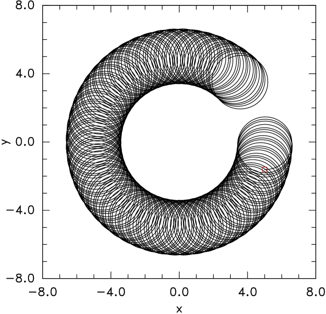
Figure 2: Example of a trapped orbit (a) projected in two dimensions showing the axisymmetric direction drift, and (b) in three dimensions showing the parallel bounce motion.

in Fig. 2. The projection of the orbit on to the transverse plane shows the drift in the axisymmetric $\theta$ direction of the circular orbit in this situation where the gyro-radius is a moderate fraction of the guiding-center radius and transverse potential scale-length. Simultaneously the orbit is bouncing in the parallel direction, as shown by the three-dimensional perspective. The shape of the potential in which this particle is moving is given by the contours of Fig. 1.

In Fig. 3 is shown the variation of some other parameters of the orbit.

Figure 3: Orbit evolution, showing the particle radius (red) and gyro-averaged radius (green) as a function of parallel position $z$ (top panel), and the parallel energy $W_{\parallel}$ (red) and its gyro-average $\bar{W}_{\parallel}$ (green) together with the potential at the guiding-center ($r_{c0}$) and minimum radius $r_{min}$ (second and third panels). See text for detailed explanation.

The top panel shows the instantaneous radial position $r(z)$ (red) and its single-gyro-period running gyro-average $\bar{r}$ (green). The dashed line is the initial radial position of the orbit’s guiding-center (a chosen parameter $r_{c0}$ for this orbit). [Because there are many bounces of the orbit, individual lines are hard to discern except at large magnification.] Also shown are the initial particle position $r_{0}$ (square) and the positions of the nominal extrema of the orbit based on the initial gyro-radius, namely $r_{c0}\pm r_{g0}$ (triangle and circle). For this example the gyro-averaged radius $\bar{r}$ has very small excursions. On average $\bar{r}$ slightly exceeds $r_{c0}$. The initial particle radius exceeds even $\bar{r}$, but is controlled by the initial gyro-phase (a chosen parameter), which in this case is that the initial velocity is directed along the guiding-center radius from the origin; so $r^{2}_{0}=r_{c0}^{2}+r_{g0}^{2}$ .

The second panel shows the instantaneous and running gyro-averaged value of the parallel energy $W_{\parallel}=v_{\parallel}^{2}/2-\phi(r,z)$. Because of the gyration up and down the substantial radial potential gradient, the perpendicular kinetic energy $W_{\perp}=v_{\perp}^{2}/2$ varies considerably with gyro-angle. Consequently $W_{\parallel}=W-W_{\perp}$ varies by an equal and opposite amount, since $W$ is exactly conserved. (In the code $W$ is monitored and confirms accuracy to a fraction level of $\sim 10^{-5}$.) Even though $W_{\parallel}$ can instantaneously exceed zero, the orbit remains trapped for in excess of 200 parallel bounces. The gyro-averaged $\bar{W}_{\parallel}$ shows some limited variation with $z$ and gyro-angle, but remains below zero; so the orbit remains trapped. The lowest panel plots, in addition to $W_{\parallel}$, the potential energy at $r_{c0}$ and $r_{min}$. One can observe that the $z$-extrema of the orbit are approximately where $\bar{W}_{\parallel}=-\phi(r_{c0})$ and $W_{\parallel min}=-\phi(r_{min})$ corresponding to zero parallel kinetic energy.

Fig. 4 shows for comparison an orbit in exactly the same potential (whose peak is $\psi_{0}=0.16$) and magnetic field strength ($\Omega=0.9$), and the same total energy ($W=1$), but with a starting parallel energy that is closer to the trapped-passing boundary ($W_{\parallel}=-0.13\psi(r_{c0})$ instead of $-0.5\psi(r_{c0})$).

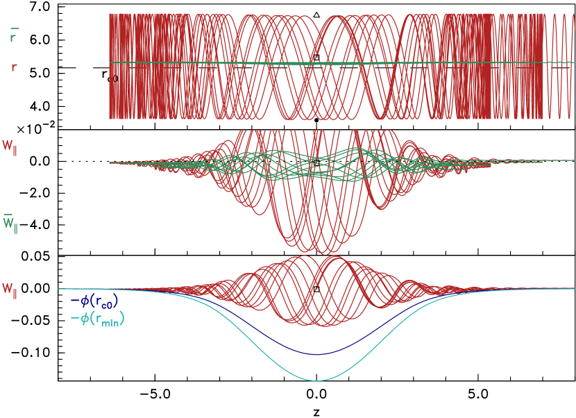
Figure 4: Orbit evolution for a more shallowly trapped orbit than Fig. 3, but otherwise the same parameters.

The orbit starts trapped, but only just. Consequently its parallel excursions extend farther out in $|z|$. Focusing (at high resolution) on the green line in the second panel $\bar{W}_{\parallel}$, one can see that the first bounce position (at positive $z$) is at $|z|\simeq 4.5$ and $\bar{W}_{\parallel}\simeq-0.07\times 10^{-2}$. However each subsequent bounce occurs at an increasing value of $|z|$ because $\bar{W}_{\parallel}$ increases toward zero, until after 10 bounces it becomes positive and the orbit escapes the hole, moving out to large positive $z$. In the inner regions of the hole, $\bar{W}_{\parallel}$-variation with gyro-angle is very significant, but at the ends near the bounce the excursions become small, because the radial potential gradient is small there, and it is naturally the value at the ends that determines whether the particle bounces or not.

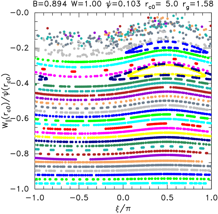
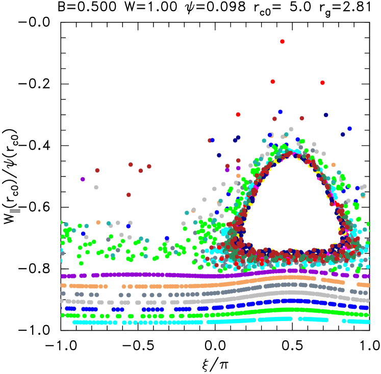
Figure 5: Poincaré plot of the parallel energy and gyro-angle at passages through $z=0$ for the potential form of Fig. 1. (a) for the magnetic field strength $\Omega=0.9$ of Figs. 2, 3 and 4, (b) for a lower magnetic field, $\Omega=0.5$.

In Fig. 5(a) is shown a Poincaré plot of the parallel energy, $W_{\parallel}(r_{c0})$, evaluated taking the potential to be that at position $r_{c0}$ (which is a proxy for the gyro-averaged potential ignoring $\partial^{2}\phi/\partial r^{2}$ requiring no averaging), against the gyro-angle for each passage of an orbit through $z=0$. A sequence of starting $W_{\parallel}$ orbits is shown in a corresponding sequence of colors. The orbit of Fig. 3 corresponds to $W_{\parallel}(r_{c0})/\psi(r_{c0})\simeq-0.5$. At that energy all the orbits are permanently trapped and no obvious phase-space islands are observed. The ratio of the gyro-frequency $\Omega$ to twice the bounce frequency $2\omega_{b}$ there is approximately 3.5, so it is not close to a bounce-cyclotron resonance ($\ell\omega_{b}=\Omega$ with $\ell$ an even integer). The nearest resonance is $\ell=8$ at $W_{\parallel}(r_{c0})/\psi(r_{c0})\simeq-0.35$ where an island is obvious. By contrast, the orbit of Fig. 4 corresponds to a starting energy $W_{\parallel}(r_{c0})/\psi(r_{c0})\simeq-0.13$ which is in the region of apparently stochastic orbits just below the zero of energy. It corresponds closely to the purple orbit in that region, which only has a few points because it quickly becomes detrapped. Its energy is just above that for the $\ell=12$ and 14 resonances. Actually the progressive gyro-averaged energy increase observed in Fig. 4 does not require the orbit literally to be stochastic in order to become detrapped. But nevertheless detrapping like this is observed to take place mostly in proximity to parameters that have overlapped islands and stochastic orbits. Regions of detrapping (which are also, by time reversal, regions of trapping) and stochasticity experience strong effective energy diffusion which will limit any gradients in $f_{\parallel}$ and hence suppress $\tilde{f}$. In this case, a distribution in which $\tilde{f}\simeq 0$ down to $W_{\parallel}(r_{c0})/\psi(r_{c0})\simeq-0.25$ would be plausible, but not one that called for substantially non-zero $\tilde{f}$ closer to $W_{\parallel}=0$.

Fig. 5(b) shows what happens if the magnetic field strength is lowered but with all else the same. The gyro-resonance energy is changed so that the $\ell=4$ island centered on $W_{\parallel}(r_{c0})/\psi(r_{c0})\simeq-0.6$ comes to dominate the Poicaré plot. In this case making the initial gyro-averaged potential negative does not represent well the trapping condition, because almost all energies above the resonance are detrapped. In fact all orbits with $W_{\parallel}(r_{c0})/\psi(r_{c0})>-0.26$ are lost immediately without even a single bounce, because the gyro-averaged potential happens to rise above zero in the first quarter of the bounce period for all such orbits with the standard starting gyro-phase. At different starting gyro-phase one can find higher energy orbits with a few (up to 10) bounces prior to loss, but the overall lost region (whether after zero or a few bounces) of phase-space is essentially the same. High enough magnetic field avoids such strong resonances.

Further trends with guiding-center position are illustrated in Fig. 6, where different guiding-center position ($r_{c0}$) cases are shown for the same hole parameters as Fig. 5(b).

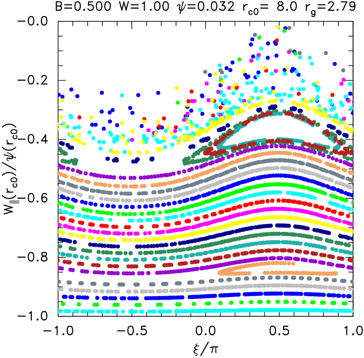
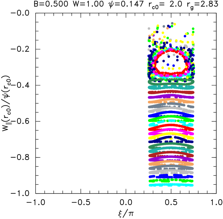
Figure 6: Poincaré plots at different guiding-center radii, and the lower magnetic field.

Fig. 6(a) is for a larger guiding-center radial position $r_{c0}=8$ in the exponentially decaying radial wing of the hole where the peak potential $\psi$ is substantially smaller. It has considerably less of its phase-space detrapped than Fig. 5(b). Fig. 6(b) shows instead a case where $r_{c0}<r_{g}$ so that the gyro-orbit itself encircles the origin ($r=0$). The resulting excursion of the gyro-phase $\xi$ (which is defined as the angle between the perpendicular velocity and the particle radius vector from the origin) is now less than $2\pi$. It also, though, shows a region of detrapping that is comparable to Fig. 6(a) and shallower than 5(b). Thus the intermediate radii where $r_{c0}$ lies in the steep radial gradient of the potential, exemplified by 5(b), are the most susceptible to stochastic detrapping. The extreme limit of the origin-encircling orbit type is when $r_{c0}=0$, and the orbit becomes a circle centered on the origin. There are then no resonant effects and no detrapping because the orbit phase never changes.

What Figs. 4 and 5 validate is that combining the gyro-averaged potential energy ($-\bar{\phi}$) plus the parallel kinetic energy $v_{\parallel}^{2}/2$ gives a quantity $\bar{W}_{\parallel}$ whose sign rather accurately determines whether or not an orbit bounces; and that, although this quantity has significant excursions as the orbit moves through the low-$|z|$ strong potential regions, those do not generally lead to detrapping unless there is systematic or stochastic enhancement of the $\bar{W}_{\parallel}$ at the bounce positions due to bounce-gyro resonance.

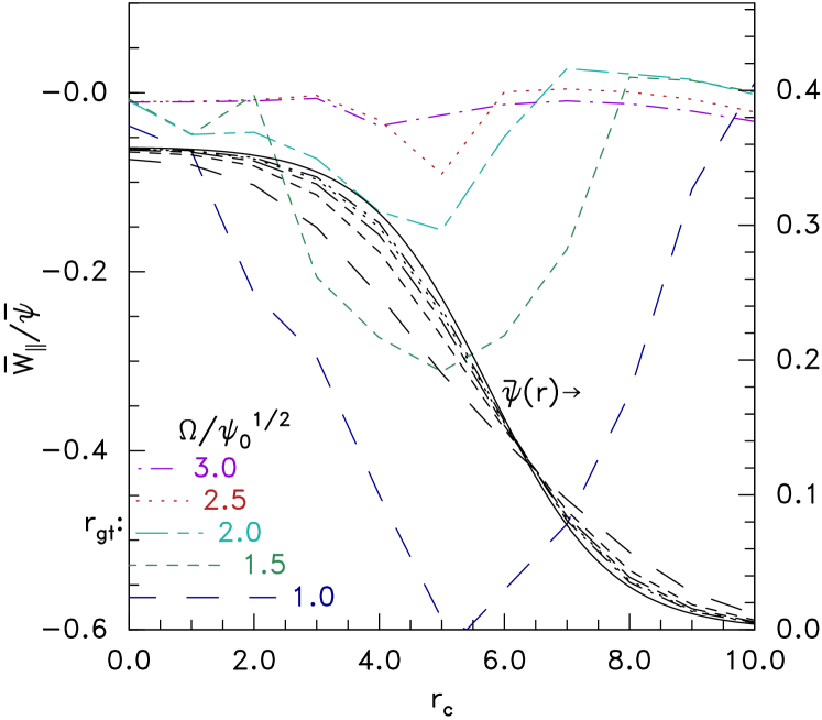
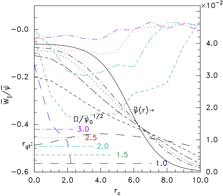
Figure 7: Highest permanently trapped orbit initial parallel energy $\bar{W}_{\parallel}$ (colors) divided by gyro-averaged potential $\bar{\psi}$, as a function of guiding-center radius for different magnetic fields indicated by the length of the thermal gyro-radius and the value of $\Omega/\psi^{1/2}$. Also radial profile of $\psi$ and $\bar{\psi}$ (black). Hole origin potential: (a) $\psi_{0}=0.36$, (b) $\psi_{0}=0.04$.

This finding is summarized by results for a large number of orbits in Fig. 7. It shows as a function of guiding-center radial position, by colored lines the maximum value of the ratio of initial parallel energy $\bar{W}$ to gyro-averaged potential $\bar{\psi}$ (both at $z=0$) for which the orbit is permanently trapped. Each plot shows cases for five different magnetic field strengths. That strength is indicated by the length of the thermal gyro-radius horizontal bars at the bottom left. It is also given by the labels consisting of the value of $\Omega/\psi_{0}^{1/2}$, which is a proxy for $\Omega/\omega_{b}$ at the hole origin and organizes the results. The radial profile of the peak potential $\psi(r)$ and the corresponding gyro-averaged potential $\bar{\psi}$ (to which $\bar{W}$ is normalized in the colored lines) is also plotted in black with the scale on the right. The different line styles correspond to the different gyro-radii. Plots have potential at the origin (a) $\psi_{0}=0.36$ and (b) $\psi=0.04$, differing by a factor of nine. Yet generally, within the uncertainty implied by the fluctuations of the curves, they tell the same story. At high magnetic field, the ratio $\bar{W}_{\parallel}/\bar{\psi}$ is close to zero, indicating that the gyro-averaged potential determines parallel trapping over the entire radial profile for all gyro-radii and $\psi_{0}$: a key result. This limit is approached when $\Omega/\psi_{0}^{1/2}\gtrsim 2$. For lower magnetic fields, detrapping by gyro-bounce resonance begins at significantly lower $\bar{W}_{\parallel}$, strongest in the central regions of largest $E_{\perp}(-d\psi/dr)$, but eventually deep detrapping occurs across most of the hole radius. Smaller amplitude ($\psi$) holes allow larger gyro-radius to be accommodated before deep detrapping sets in: Fig. 7(b).

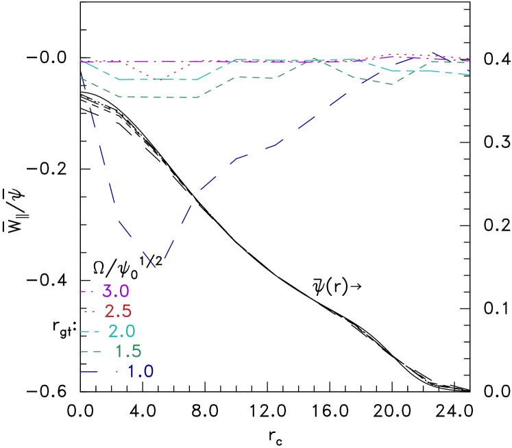
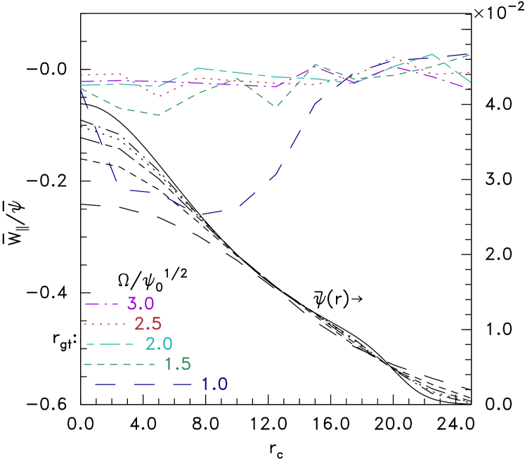
Figure 8: Highest permanently trapped orbit initial parallel energy $\bar{W}_{\parallel}$ divided by gyro-averaged potential $\bar{\psi}$, as in Fig. 7 except with a more peaked radial profile extending to much larger radius.

Fig. 8 shows a much wider but more peaked radial profile case. Detrapping is now strongest relatively close to the potential peak, which is where the radial field is strongest. A threshold below which gyro-bounce resonance causes major detrapping is still present. It is quantitatively at somewhat lower ratio $\Omega/\sqrt{\psi}_{0}\sim 1$, in part because of the $E_{r}$ reduction.

The $\bar{\psi}$ curves of Figs. 7 and 8 illustrate how gyro-averaging is changing the effective potential, lowering it near $r=0$, and raising it in the positive curvature wings.

IV The consequences of gyro-averaging and resonance detrapping

The key consequence of gyro-averaging is that trapped density deficits become less effective at sustaining the hole potential. That reduced effectiveness requires deeper deficits in order to sustain the same potential, leading eventually to a violation of non-negativity of the distribution function. It is easiest and most relevant to think of this in terms of the convolution spreading of the potential profile given $\tilde{n}(r)$.

A Gaussian radial potential profile $\psi(r)=\psi_{0}{\rm e}^{-(r/a)^{2}/2}$ provides the simplest illustration of what gyro-averaging does. When convolved with the Gaussian of width $\sqrt{2}r_{gt}$ it yields a modified finite-gyro-radius Gaussian profile $\bar{\psi}(r)$ of greater width $\sqrt{a^{2}+2r_{gt}^{2}}$. Of course the total volume $\int_{0}^{\infty}\psi(r)2\pi rdr$ is conserved during convolution, consequently the height of the smoothed $\bar{\psi}$ is smaller by the ratio $\bar{\psi}_{0}/\psi_{0}=(1+2r_{gt}^{2}/a^{2})^{-1}$. This factor gives a strong reduction of the potential height at the origin once $2r_{gt}$ exceeds $a$. The same spreading occurs for any shape of profile $\psi(r)$, when its width is considered to be given by the variance $\langle r^{2}\rangle=\int_{0}^{\infty}r^{2}\psi(r)2\pi rdr/\int_{0}^{\infty}\psi(r)2\pi rdr$. For a Gaussian of width $a$, $\langle r^{2}\rangle=2a^{2}$. For a general profile, when it is convolved with a Gaussian of width $\sqrt{2}r_{gt}$, its variance increases as $\langle\bar{r}^{2}\rangle=\langle r^{2}\rangle+4r_{gt}^{2}$. The difference is that for a non-Gaussian initial profile its relative shape changes (toward Gaussian) when convolved, and so the ratio of central heights $\bar{\psi}_{0}/\psi_{0}$ is not exactly the same, even though the ratio of the average heights is the same $(\int\bar{\psi}2\pi rdr/\langle\bar{r}^{2}\rangle)/(\int\psi 2\pi rdr/\langle r^{2}\rangle)=(1+2r_{gt}^{2}/a^{2})^{-1}$. We shall take the average height suppression to represent the main effect. This amounts to supposing (correctly) that the inner regions of the hole are the most important.

The relative importance of the two main multidimensional electron hole modifications, gyro-averaging and transverse electric field divergence, can be estimated by writing the field divergence $\nabla^{2}\phi\sim-(a^{-2}+L_{\parallel}^{-2})\phi$. The potential is thus suppressed by divergence in a hole of transverse dimension $\sim a$ relative to a one-dimensional hole with the same charge density by a factor $F_{\perp}^{-1}\sim(1+L_{\parallel}^{2}/a^{2})^{-1}$ where $L_{\parallel}$ is a parallel scale length $\sim\lambda_{D}$ (1 in normalized units). The gyro-average potential spreading factor $(1+2r_{gt}^{2}/a^{2})^{-1}$ thus becomes more important than the effects of transverse electric field divergence when $r_{g}\gtrsim\lambda_{D}$ that is $\omega_{p}\gtrsim\Omega$ or $\Omega\lesssim 1$ in normalized units. Since the threshold of strong depletion by gyro-bounce resonance effects is $\Omega\sim 2\psi^{1/2}$, a hole depth $\psi$ much smaller than 1 (times $T_{e}$) will be more strongly suppressed by gyro-averaging than by transverse divergence, near the gyro-bounce threshold. This point is made more quantitative in the following.

IV.1 Relationship between electron distribution deficit and potential

Poisson’s equation relates the potential and the electron distribution (with the ions as an immobile unity background charge density). Integrating it along the parallel direction requires that

$$\begin{split}0={1\over 2}\left.\left(\partial\phi\over\partial z\right)^{2}\right|_{z=0}&=\int_{\infty}^{0}(n(\phi)-1-\nabla_{\perp}^{2}\phi){\partial\phi\over\partial z}dz\\ &\approx-\tilde{V}+(1-\langle\nabla_{\perp}^{2}\rangle)\psi^{2}/2,\end{split}$$ (6)

where we have written $-\tilde{V}\equiv\int\tilde{n}d\phi$, $\langle\nabla_{\perp}^{2}\rangle\equiv 2\int\nabla_{\perp}^{2}\phi d\phi/\psi^{2}$, and $n(\phi)=n_{f}+\tilde{n}$ is the sum of a reference distribution that is independent of parallel velocity in the trapped region and $\tilde{n}$ is the deficit of the trapped electron density with respect to it. The final equality of eq. (6) approximates $n_{f}\simeq 1+\phi$ and approximates the potential form as separable. $\nabla_{\perp}^{2}\phi/\phi$ is then a function only of $r$ and equal to $\langle\nabla_{\perp}^{2}\rangle$ which can be taken out of the $z$-integral; for non-separable potential it must remain in integral form. Since $\tilde{n}=\int_{0}^{\sqrt{2\phi}}\tilde{f}dv$, the classical potential $\tilde{V}$ scales like $\sim-\tilde{f}\psi^{3/2}$, and eq. (6) means $-\tilde{f}\sim(1-\langle\nabla_{\perp}^{2}\rangle)\psi^{1/2}$. This scaling is universal.

In the “power deficit model”, worked out in detail elsewhereHutchinson (2021a), the trapped parallel distribution deficit $\tilde{f}$ is presumed to be of the specific form

$$\tilde{f}(W_{\parallel})=\tilde{f}_{\psi}\left(W_{j}-W_{\parallel}\over W_{j}+\phi\right)^{\alpha}$$ (7)

varying between zero at parallel energy $W_{\parallel}=v_{\parallel}^{2}/2-\phi=W_{j}$ and $\tilde{f}_{\psi}$ at parallel energy $W_{\parallel}=-\psi$ (the bottom of the potential well). Fractional powers of negative quantities are by convention taken to be zero, so there is zero deficit for energies $W_{\parallel}>W_{j}$, i.e. near the trapped-passing boundary $W_{\parallel}=0$. In the absence of gyro-averaging, the condition (6) on the classical potential $V=\int\rho{d\phi\over dz}dz$ for the power deficit model has analytic coefficients and becomes:

$$-\tilde{f}_{\psi}\psi^{3/2}(1+W_{j}/\psi)^{3/2}{2G\over\alpha+3/2}=-F_{\perp}V_{f}(\psi)\simeq F_{\perp}\psi^{2}/2.$$ (8)

Here $G=\sqrt{\pi/2}\Gamma(\alpha+1)/\Gamma(\alpha+3/2)$ is a constant depending only on $\alpha$, expressible in terms of the Gamma function, $V_{f}(\phi)$ is the classical potential of the flat-trapped screening density $n_{f}\simeq 1+\phi$ minus the background uniform ion density, and $F_{\perp}$ is the local correction factor $F_{\perp}(r)=(1-\langle\nabla_{\perp}^{2}\rangle)$ that accounts for perpendicular electric field divergence in Poisson’s equation. Now $F_{\perp}$ and $V_{f}(\phi)\simeq-\phi^{2}/2$ are unaltered by gyro-averaging because they depend on the local, not gyro-averaged, potentialHutchinson (2021b). But the left hand side term $\tilde{f}_{\psi}(\psi+W_{j})^{3/2}$ represents the trapped electron guiding-center distribution deficit integrated with respect to $\bar{\phi}$, and must account for gyro-averaging. So in the presence of finite gyro radius it must be taken as $\tilde{f}_{c\bar{\psi}}(\bar{\psi}+\bar{W}_{j})^{3/2}$, and on average $\bar{\psi}/\psi\simeq(1+4r_{gt}^{2}/\langle r^{2}\rangle_{0})^{-1}$. We will suppose that $\bar{W}_{j}/\bar{\psi}=W_{j}/\psi$ is independent of gyro-averaging. If instead $\bar{W}_{j}=W_{j}$ were kept constant as $\psi$ was averaged, the constraints about to be discussed would be made more severe.

To compensate for the reduction in trapped energy range caused by $\bar{\phi}$ averaging reduction, if we wished to preserve $\psi(r)$ while increasing $r_{gt}$, the condition (8) then requires a greater trapped guiding-center deficit

$$\tilde{f}_{c\bar{\psi}}=\tilde{f}_{\psi}(1+4r_{gt}^{2}/\langle r^{2}\rangle)^{3/2}.$$ (9)

The resulting cubic dependence of $|\tilde{f}_{c\bar{\psi}}|$ on $r_{gt}$, if $r_{gt}^{2}/\langle r^{2}\rangle$ is allowed to increase significantly beyond unity by lowering the magnetic field strength, will soon cause the trapped electron deficit to exceed the allowed maximum value (0.399) permitted by non-negativity of the total guiding-center distribution function. Non-negativity therefore constrains ${\langle r^{2}\rangle}$ not to be very much smaller than $r_{gt}^{2}$. An alternative way to accommodate gyro-averaging increase might be to decrease $\psi$, thereby reducing the required $|\tilde{f}_{c\bar{\psi}}|$. However, if the magnitude of $|\tilde{f}_{c\bar{\psi}}|$ is fixed by non-negativity, then eq. (9) requires $\psi\sim(1+4r_{gt}^{2}/\langle r^{2}\rangle)^{-3}$, an even stronger (sixth power) dependence on gyro-radius, which would rapidly force the hole potential to become negligible. We can conclude that electron hole equilibria exist in the presence of gyro-averaging only if increase of gyro-radius is accompanied by increase of transverse potential extent approximately keeping pace with gyro-radius. Or expressed more briefly: $4r_{gt}^{2}\lesssim\langle r^{2}\rangle$. Although we have demonstrated this effect for a particular model of the parallel distribution, the scalings, if not the precise coefficients, of all the phenomena are virtually independent of the model or the transverse profiles.

It should be remarked that the empirical scaling of Franz et al, $L_{\perp}/L_{\parallel}\sim\sqrt{1+(\omega_{p}/\Omega)^{2}}$, is in the present terminology $\langle r^{2}\rangle=L_{\parallel}^{2}(1+1/\Omega^{2})=L_{\parallel}^{2}(1+r_{gt}^{2})$, and taking $L_{\parallel}=2$ is indistinguishable (within their significant observational uncertainty) from $\langle r^{2}\rangle=4r_{gt}^{2}$.

IV.2 Allowable electron hole parameter space

Let us write equation (8) at the origin (the most demanding place) with the maximum allowable $-\tilde{f}_{c\bar{\psi}_{0}}=1/\sqrt{2\pi}$ to avoid a negative distribution function. Since we are focussing on $r=0$, take the transverse potential shape there to be approximately Gaussian $\propto{\rm e}^{-(r/a)^{2}/2}\simeq 1-(r/a)^{2}/2$ with width $a=\langle r^{2}\rangle^{1/2}_{0}/\sqrt{2}$ and $\langle\nabla_{\perp}^{2}\rangle_{0}=-2/a^{2}$, so the divergence and gyro-averaging factors are $(1+2/a^{2})[1+2/(\Omega^{2}a^{2})]^{3/2}$. Then

$$\psi_{0}^{1/2}={(1+W_{j}/\psi)^{3/2}\over(1+2/a^{2})[1+2/(\Omega^{2}a^{2})]^{3/2}}{2G\over\sqrt{\pi/2}(\alpha+3/2)}.$$ (10)

Now at the maximum permissible value of $(1+W_{j}/\psi)$, the coefficient $(1+W_{j}/\psi)^{3/2}2G/(a+3/2)$ is approximately 2.4 at $\alpha=0$ and falls to about 1.2 at $\alpha=1$ because of the $z$-peaking of the profile. If we adopt the $\alpha=0$ value (the most forgiving) and write $2.4/\sqrt{\pi/2}\simeq 2$ for the total coefficient we obtain for the maximum allowable potential

$$\psi_{0}\simeq 4(1+2/a^{2})^{-1}[1+2/(\Omega a)^{2}]^{-3}.$$ (11)

This gives the maximum of $\psi_{0}$ versus $\Omega$ for some chosen $a$. Lines below which $\psi_{0}$ must lie are shown for a range of widths $a$ in Fig. 9

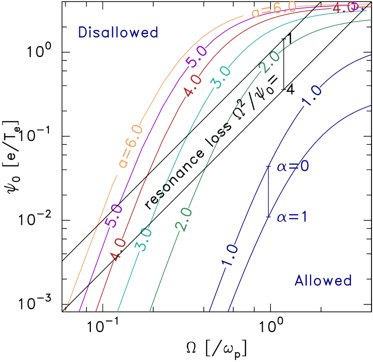
Figure 9: The limits of allowable peak potential permitted by non-negativity of $f$ (colors) and avoidance of gyro-bounce resonant detrapping (black). Non-negativity depends on the radial width $a=(-\langle\nabla_{\perp}^{2}\rangle_{0}/2)^{-1/2}$. It also varies depending on the parallel-peaking coefficient $\alpha$; curves are highest for a waterbag deficit $\alpha=0$. The range is indicated by the vertical bar. The approximate uncertainty range of the resonance loss is indicated similarly. The parameters must lie below both relevant lines.

For $\alpha=1$ the lines shift downward by a factor $\sim 4$ as shown by the bar and associated line for $a=1$. Permissible equilibria lie below the lines. Obviously points for which $-\tilde{f}_{\psi}$ is actually less than $1/\sqrt{2\pi}$, so the total trapped distribution is greater than zero, lie below the line by an additional factor, which is $-\tilde{f}_{\psi}^{2}2\pi$.

The other major constraint on equilibrium is the detrapping of electrons by gyro-bounce resonance. Based on the prior studies of exponential potential gradientsHutchinson (2020), $\psi_{0}$ must lie below $\psi_{0}\sim\Omega^{2}/4$ to avoid strong detrapping. The explorations of section III (Fig. 8) show that for wider holes with lower peak gradients the limit is closer to $\psi_{0}\sim\Omega^{2}$. These limit lines give the typical range of resonance loss thresholds, shown by two black straight lines in Fig. 9. The strong detrapping effects take place not at $r=0$ but in the steep region of the potential profile; even so, they prevent a steady equilibrium shape having $\psi_{0}$ above the threshole, and actually tend to shrink the transverse width, making the losses worse and tending to collapse the hole entirely.

V Discussion

The theory described here has addressed the three main effects of finite transverse extent on electron hole equilibria (1) transverse electric field divergence, (3) orbit detrapping by gyro-bounce resonance, and (4) gyro-averaging effects on the potential and density deficit. [Supposed modification of the shielding, enumerated (2) in the introduction, does not occur.] It has explored a sampling of different self-consistent transverse shapes.

In addition to the plausibility constraint that the distribution deficit $\tilde{f}$ should be zero at and immediately below the trapped-passing boundary, the two critical physics constraints of non-negativity and avoidance of resonant detrapping have been applied to obtain bounds relating the peak potential $\psi_{0}$, magnetic field strength $\Omega$ (equivalent to the inverse of the thermal gyro-radius $r_{gt}$), and the transverse extent $a\ (=\sqrt{\langle r^{2}\rangle/{2}})$. Fig. 9 shows these limits graphically.

The convenient specialization of the current work to axisymmetric geometry has avoided complications associated with fully three dimensional structures. The principles of gyro-averaging of potential and of particle deficit, and the principles of gyro-bounce orbit detrapping, will apply fully regardless of non-axisymmetry. Since gyro-orbits remain circular in the drift frame, their averaging remains isotropic in the transverse plane, and the effective adjustment depends to lowest order on the transverse Laplacian of the unaveraged potential. The gyro-bounce detrapping perturbation depends on the potential through the magnitude, not direction, of its gradient. Since in the wings Debye shielding gives rise to $|\nabla_{\perp}\phi/\phi|\simeq 1$ it is expected to have similar behavior there regardless of non-axisymmetry. The central regions expected to be most susceptible to resonant detrapping would be those where the transverse gradient is largest. However, the dependence of detrapping on $E_{\perp}$ is weaker than its dependence on $\Omega/\sqrt{\psi}$ until $E_{\perp}$ becomes very small. Overall, since Fig. 9 is independent of hole geometry apart from the parameter $a$, whose inverse equals the square root of the normalized Laplacian ($\sqrt{\nabla_{\perp}^{2}\phi/\phi}$) at the origin, it may be expected to apply to non-axisymmetric electron holes to approximately the same degree that it applies to axisymmetric ones.

It should be recognized that while non-negativity and Poisson’s equation are instantaneous requirements, resonant detrapping takes a significant time to deplete the trapped deficit: typically some moderate number of bounce-times, and certainly at least $\sim$ the gyro-period. Therefore, if a multidimensional electron hole is formed approximately in a bounce-time or faster, for example by a highly nonlinear bump-on tail instability or some subsequent process such as transverse break-up of an initially one-dimensional hole, then it takes a longer time for the resonant detrapping to become important. It might then be possible to observe multidimensional electron holes shortly after their formation that violate the resonant detrapping criterion. Indeed, avoiding all resonance loss is such a severe requirement that it prevents the long term sustainment of multidimensional electron holes of any significant potential amplitude (e.g. $\psi_{0}>10^{-2}T_{e}/e$) below magnetic field strength corresponding to $\Omega/\omega_{p}\sim 0.1$. The present results thus suggest that any solitary potential structures observed in space plasmas where $\Omega/\omega_{p}\lesssim 0.1$ are either some phenomenon different from electron holes, or they are just-formed electron holes that will quite soon disappear by resonant detrapping.

The gyro-averaging effects combined with non-negativity act in a shorter time. Above the green curves of Fig. 9, orbits escape in approximately a quarter of a bounce period. This duration is so short that such a situation, violating the constraint, cannot be considered a Vlasov equilibrium, because $f$ is not a function of energy. It is also much less likely that such an object would be observed, because of its short life. If then the resonance loss constraint (black curve) was violated for some moderate time duration, but the non-negativity constraint was not, and became the determining factor, then the simplified theoretical scaling $\langle r^{2}\rangle\gtrsim 4r_{gt}^{2}$ would be expected. Equality in this equation is indistinguishable from the empirical scaling of Franz et alFranz et al. (2000). Nevertheless the experimental proxy they used for aspect ratio ($E_{\parallel}/E_{\perp}$) has been shownHutchinson (2021a) to be an extremely uncertain measure of $L_{\perp}/L_{\parallel}$; so one should not make too much of this agreement with observations. A great deal remains to be done to establish observationally what the structure of multidimensional holes in space actually is. One can look forward to a critical comparison of the theory presented here with future observations.

Acknowledgements and Supporting Material

I am grateful to Greg Hammett for helpful discussions of the foundations of gyrokinetics, to David Malaspina for insights into the instrumentation and data of satellite measurements, and to Ivan Vasko for discussions of electron hole interpretation of space observations. The code used to generate the equilibria is available at https://github.com/ihutch/helmhole, and the orbit-following code at https://github.com/ihutch/AxisymOrbits. Figures were generated by these codes or the explicit equations in the article, not from separate data. No public external funding for this research was received.

References

- Matsumoto et al. (1994) H. Matsumoto, H. Kojima, T. Miyatake, Y. Omura, M. Okada, I. Nagano, and M. Tsutsui, “Electrostatic solitary waves (ESW) in the magnetotail: BEN wave forms observed by GEOTAIL,” Geophysical Research Letters 21, 2915–2918 (1994).
- Ergun et al. (1998) R. E. Ergun, C. W. Carlson, J. P. McFadden, F. S. Mozer, L. Muschietti, I. Roth, and R. J. Strangeway, “Debye-Scale Plasma Structures Associated with Magnetic-Field-Aligned Electric Fields,” Physical Review Letters 81, 826–829 (1998).
- Bale et al. (1998) S. D. Bale, P. J. Kellogg, D. E. Larsen, R. P. Lin, K. Goetz, and R. P. Lepping, “Bipolar electrostatic structures in the shock transition region: Evidence of electron phase space holes,” Geophysical Research Letters 25, 2929–2932 (1998).
- Mangeney et al. (1999) A. Mangeney, C. Salem, C. Lacombe, J.-L. Bougeret, C. Perche, R. Manning, P. J. Kellogg, K. Goetz, S. J. Monson, and J.-M. Bosqued, “WIND observations of coherent electrostatic waves in the solar wind,” Annales Geophysicae 17, 307–320 (1999).
- Pickett et al. (2008) J. S. Pickett, L.-J. Chen, R. L. Mutel, I. W. Christopher, O. Santolı´k, G. S. Lakhina, S. V. Singh, R. V. Reddy, D. A. Gurnett, B. T. Tsurutani, E. Lucek, and B. Lavraud, “Furthering our understanding of electrostatic solitary waves through Cluster multispacecraft observations and theory,” Advances in Space Research 41, 1666–1676 (2008).
- Andersson et al. (2009) L. Andersson, R. E. Ergun, J. Tao, A. Roux, O. Lecontel, V. Angelopoulos, J. Bonnell, J. P. McFadden, D. E. Larson, S. Eriksson, T. Johansson, C. M. Cully, D. N. Newman, M. V. Goldman, K. H. Glassmeier, and W. Baumjohann, “New features of electron phase space holes observed by the THEMIS mission,” Physical Review Letters 102, 225004 (2009).
- Wilson et al. (2010) L. B. Wilson, C. A. Cattell, P. J. Kellogg, K. Goetz, K. Kersten, J. C. Kasper, A. Szabo, and M. Wilber, “Large-amplitude electrostatic waves observed at a supercritical interplanetary shock,” Journal of Geophysical Research: Space Physics 115, A12104 (2010).
- Malaspina et al. (2013) D. M. Malaspina, D. L. Newman, L. B. Willson, K. Goetz, P. J. Kellogg, and K. Kerstin, “Electrostatic solitary waves in the solar wind: Evidence for instability at solar wind current sheets,” Journal of Geophysical Research: Space Physics 118, 591–599 (2013).
- Malaspina et al. (2014) D. M. Malaspina, L. Andersson, R. E. Ergun, J. R. Wygant, J. W. Bonnell, C. Kletzing, G. D. Reeves, R. M. Skoug, and B. A. Larsen, “Nonlinear electric field structures in the inner magnetosphere,” Geophysical Research Letters 41, 5693–5701 (2014).
- Vasko et al. (2015) I. Y. Vasko, O. V. Agapitov, F. Mozer, A. V. Artemyev, and D. Jovanovic, “Magnetic field depression within electron holes,” Geophysical Research Letters 42, 2123–2129 (2015).
- Mozer et al. (2016) F. S. Mozer, O. A. Agapitov, A. Artemyev, J. L. Burch, R. E. Ergun, B. L. Giles, D. Mourenas, R. B. Torbert, T. D. Phan, and I. Vasko, “Magnetospheric Multiscale Satellite Observations of Parallel Electron Acceleration in Magnetic Field Reconnection by Fermi Reflection from Time Domain Structures,” Physical Review Letters 116, 4–8 (2016), arXiv:arXiv:1011.1669v3 .
- Hutchinson and Malaspina (2018) I. H. Hutchinson and D. M. Malaspina, “Prediction and Observation of Electron Instabilities and Phase Space Holes Concentrated in the Lunar Plasma Wake,” Geophysical Research Letters 45, 3838–3845 (2018).
- Mozer et al. (2018) F. S. Mozer, O. V. Agapitov, B. Giles, and I. Vasko, “Direct Observation of Electron Distributions inside Millisecond Duration Electron Holes,” Physical Review Letters 121, 135102 (2018).
- Bernstein, Greene, and Kruskal (1957) I. B. Bernstein, J. M. Greene, and M. D. Kruskal, “Exact nonlinear plasma oscillations,” Physical Review 108, 546–550 (1957).
- Hutchinson (2017) I. H. Hutchinson, “Electron holes in phase space: What they are and why they matter,” Physics of Plasmas 24, 055601 (2017).
- Mottez et al. (1997) F. Mottez, S. Perraut, A. Roux, and P. Louarn, “Coherent structures in the magnetotail triggered by counterstreaming electron beams,” Journal of Geophysical Research 102, 11399 (1997).
- Miyake et al. (1998) T. Miyake, Y. Omura, H. Matsumoto, and H. Kojima, “Two-dimensional computer simulations of electrostatic solitary waves observed by Geotail spacecraft,” Journal of Geophysical Research 103, 11841 (1998).
- Goldman, Oppenheim, and Newman (1999) M. V. Goldman, M. M. Oppenheim, and D. L. Newman, “Nonlinear two-stream instabilities as an explanation for auroral bipolar wave structures,” Geophysical Research Letters 26, 1821–1824 (1999).
- Oppenheim, Newman, and Goldman (1999) M. Oppenheim, D. L. Newman, and M. V. Goldman, “Evolution of Electron Phase-Space Holes in a 2D Magnetized Plasma,” Physical Review Letters 83, 2344–2347 (1999).
- Muschietti et al. (2000) L. Muschietti, I. Roth, C. W. Carlson, and R. E. Ergun, “Transverse instability of magnetized electron holes,” Physical Review Letters 85, 94–97 (2000).
- Oppenheim et al. (2001) M. M. Oppenheim, G. Vetoulis, D. L. Newman, and M. V. Goldman, “Evolution of electron phase-space holes in 3D,” Geophysical Research Letters 28, 1891–1894 (2001).
- Singh, Loo, and Wells (2001) N. Singh, S. M. Loo, and B. E. Wells, “Electron hole structure and its stability depending on plasma magnetization,” Journal of Geophysical Research 106, 21183–21198 (2001).
- Lu et al. (2008) Q. M. Lu, B. Lembege, J. B. Tao, and S. Wang, “Perpendicular electric field in two-dimensional electron phase-holes: A parameter study,” Journal of Geophysical Research 113, A11219 (2008).
- Hutchinson (2018) I. H. Hutchinson, “Transverse instability of electron phase-space holes in multi-dimensional Maxwellian plasmas,” Journal of Plasma Physics 84, 905840411 (2018), arXiv:1804.08594 .
- Hutchinson (2019a) I. H. Hutchinson, “Transverse instability magnetic field thresholds of electron phase-space holes,” Physical Review E 99, 053209 (2019a).
- Hutchinson (2019b) I. H. Hutchinson, “Electron phase-space hole transverse instability at high magnetic field,” Journal of Plasma Physics 85, 905850501 (2019b), arXiv:1906.04065 .
- Wu et al. (2010) M. Wu, Q. Lu, C. Huang, and S. Wang, “Transverse instability and perpendicular electric field in two-dimensional electron phase-space holes,” Journal of Geophysical Research: Space Physics 115, A10245 (2010).
- Graham et al. (2016) D. B. Graham, Y. V. Khotyaintsev, A. Vaivads, and M. André, “Electrostatic solitary waves and electrostatic waves at the magnetopause,” Journal of Geophysical Research: Space Physics 121, 3069–3092 (2016).
- Steinvall et al. (2019) K. Steinvall, Y. V. Khotyaintsev, D. B. Graham, A. Vaivads, P.-A. Lindqvist, C. T. Russell, and J. L. Burch, “Multispacecraft analysis of electron holes,” Geophysical Research Letters 46, 55–63 (2019), https://agupubs.onlinelibrary.wiley.com/doi/pdf/10.1029/2018GL080757 .
- Lotekar et al. (2020) A. Lotekar, I. Y. Vasko, F. S. Mozer, I. Hutchinson, A. V. Artemyev, S. D. Bale, J. W. Bonnell, R. Ergun, B. Giles, Y. V. Khotyaintsev, P.-A. Lindqvist, C. T. Russell, and R. Strangeway, “Multisatellite mms analysis of electron holes in the earth’s magnetotail: Origin, properties, velocity gap, and transverse instability,” Journal of Geophysical Research: Space Physics 125, e2020JA028066 (2020), e2020JA028066 10.1029/2020JA028066, https://agupubs.onlinelibrary.wiley.com/doi/pdf/10.1029/2020JA028066 .
- Schamel (1979) H. Schamel, “Theory of Electron Holes,” Physica Scripta 20, 336–342 (1979).
- Chen and Parks (2002) L.-J. Chen and G. K. Parks, “BGK electron solitary waves in 3D magnetized plasma,” Geophysical Research Letters 29, 41–45 (2002).
- Muschietti et al. (2002) L. Muschietti, I. Roth, C. W. Carlson, and M. Berthomier, “Modeling stretched solitary waves along magnetic field lines,” Nonlinear Processes in Geophysics 9, 101–109 (2002).
- Chen, Thouless, and Tang (2004) L.-J. Chen, D. Thouless, and J.-M. Tang, “Bernstein–Greene–Kruskal solitary waves in three-dimensional magnetized plasma,” Physical Review E 69, 55401 (2004).
- Krasovsky, Matsumoto, and Omura (2004a) V. L. Krasovsky, H. Matsumoto, and Y. Omura, “On the three-dimensional configuration of electrostatic solitary waves,” Nonlinear Processes in Geophysics 11, 313–318 (2004a).
- Krasovsky, Matsumoto, and Omura (2004b) V. L. Krasovsky, H. Matsumoto, and Y. Omura, “Effect of trapped-particle deficit and structure of localized electrostatic perturbations of different dimensionality,” Journal of Geophysical Research: Space Physics 109, A04217 (2004b).
- Hutchinson (2021a) I. H. Hutchinson, “Synthetic multidimensional plasma electron hole equilibria,” Physics of Plasmas (2021a), submitted.
- Franz et al. (2000) J. R. Franz, P. M. Kintner, C. E. Seyler, J. S. Pickett, and J. D. Scudder, “On the perpendicular scale of electron phase-space holes,” Geophysical Research Letters 27, 169–172 (2000).
- Vasko et al. (2017) I. Y. Vasko, O. V. Agapitov, F. S. Mozer, A. V. Artemyev, J. F. Drake, and I. V. Kuzichev, “Electron holes in the outer radiation belt: Characteristics and their role in electron energization,” Journal of Geophysical Research: Space Physics 122, 120–135 (2017).
- Vasko et al. (2018) I. Y. Vasko, V. V. Krasnoselskikh, F. S. Mozer, and A. V. Artemyev, “Scattering by the broadband electrostatic turbulence in the space plasma,” Physics of Plasmas 25, 072903 (2018).
- Holmes et al. (2018) J. C. Holmes, R. E. Ergun, D. L. Newman, N. Ahmadi, L. Andersson, O. Le Contel, R. B. Torbert, B. L. Giles, R. J. Strangeway, and J. L. Burch, “Electron Phase-Space Holes in Three Dimensions: Multispacecraft Observations by Magnetospheric Multiscale,” Journal of Geophysical Research: Space Physics 123, 9963–9978 (2018).
- Tong et al. (2018) Y. Tong, I. Vasko, F. S. Mozer, S. D. Bale, I. Roth, A. V. Artemyev, R. Ergun, B. Giles, P. A. Lindqvist, C. T. Russell, R. Strangeway, and R. B. Torbert, “Simultaneous Multispacecraft Probing of Electron Phase Space Holes,” Geophysical Research Letters 45, 11,513–11,519 (2018).
- Fu et al. (2020) H. S. Fu, F. Chen, Z. Z. Chen, Y. Xu, Z. Wang, Y. Y. Liu, C. M. Liu, Y. V. Khotyaintsev, R. E. Ergun, B. L. Giles, and J. L. Burch, “First measurements of electrons and waves inside an electrostatic solitary wave,” Physical Review Letters 124, 095101 (2020).
- Hutchinson (2021b) I. H. Hutchinson, “Oblate electron holes are not attributable to anisotropic shielding,” Physics of Plasmas (2021b), accepted for publication.
- Hutchinson (2020) I. H. Hutchinson, “Particle trapping in axisymmetric electron holes,” Journal of Geophysical Research: Space Physics 125 (2020), 10.1029/2020JA028093, e2020JA028093 10.1029/2020JA028093, https://agupubs.onlinelibrary.wiley.com/doi/pdf/10.1029/2020JA028093 .
- Northrop (1961) T. G. Northrop, “The guiding center approximation to charged particle motion,” Annals of Physics 15, 79–101 (1961).