Solving a Multi-resource Partial-ordering Flexible Variant of the Job-shop Scheduling Problem with Hybrid ASP

Abstract

Many complex activities of production cycles, such as quality control or fault analysis, require highly experienced specialists to perform various operations on (semi)finished products using different tools. In practical scenarios, the selection of a next operation is complicated, since each expert has only a local view on the total set of operations to be performed. As a result, decisions made by the specialists are suboptimal and might cause significant costs. In this paper, we consider a Multi-resource Partial-ordering Flexible Job-shop Scheduling (MPF-JSS) problem where partially-ordered sequences of operations must be scheduled on multiple required resources, such as tools and specialists. The resources are flexible and can perform one or more operations depending on their properties. The problem is modeled using Answer Set Programming (ASP) in which the time assignments are efficiently done using Difference Logic. Moreover, we suggest two multi-shot solving strategies aiming at the identification of the time bounds allowing for a solution of the schedule optimization problem. Experiments conducted on a set of instances extracted from a medium-sized semiconductor fault analysis lab indicate that our approach can find schedules for 87 out of 91 considered real-world instances.

1 Introduction

Digitalization of manufacturing brings many advantages to the modern industry. Nevertheless, the work of highly experienced specialists cannot be substituted by machines in many fields like quality control, fault analysis, or research and development. In such scenarios, the experts use their knowledge of the application domain and apply sophisticated tools to perform a variety of operations on queued jobs. In absence of any automated support, the specialists select jobs and perform operations that appear to be best according to their awareness of the situation. That is, they are making locally best decisions according to numerous heuristics such as deadlines of the jobs, availability of tools and colleagues experienced in specific operations, or given preferences of jobs. However, missed deadlines of jobs, as well as the idle time of machines and experts can be very costly.

In manufacturing settings, the reduction of the operational costs is often achieved by applying automated schedulers. Job-Shop Scheduling (JSS) [johnson1954optimal] is one of the most well-known problems in which, given a set of machines and a set of jobs represented as a sequence of operations, the goal is to assign operations to machines such that: (i) each operation can be processed by one machine at a time; (ii) all jobs are processed independently of other jobs; and (iii) the execution of operations cannot be interrupted (no preemption). Practical scheduling applications resulted in various extensions of JSS, such as flexible JSS [DBLP:journals/computing/BruckerS90] in which an operation can be performed by various resources, e.g., machines or engineers; multi-resource JSS with non-linear routing [DBLP:journals/eor/Dauzere-PeresRL98], where an operation may need multiple resources for its execution, e.g., an engineer and a machine, and may have different preceding and succeeding operations. Another well-known representation is the Resource Constrained Project Scheduling Problem (RCPSP) [DBLP:journals/eor/HartmannB10], where each operation might consume some amount of available resources. Similarly, as for JSS, there are various RCPSP extensions, such as a multi-skill variant [DBLP:journals/4or/Bellenguez-Morineau08], where human resources might require skills to perform operations, or multi-mode operations [sprecher1997exact], which can be performed in different ways, e.g., using different tools and procedures.

In this paper, we consider a Multi-resource Partial-ordering Flexible JSS (MPF-JSS) problem, which can informally be described as follows: given a set of jobs, represented as partially-ordered sets of operations, and two sets of resources that can perform multiple operations, i.e., tools and engineers trained to operate them, find a schedule of operations for both machines and engineers that is optimal wrt. predefined criteria such as tardiness. The latter is defined as either $0$ if a job is done according to the computed schedule, or the difference between the completion time of this job and its deadline. The partial order of operations indicates that the sequence of some operations of a job is not important. For instance, various inspection operations using different tools are non-invasive and can be done in an arbitrary order. Selection of a specific order can, however, improve the schedule since the availability of resources, like tools or engineers, might be limited.

To solve the problem, we propose an encoding using Answer Set Programming (ASP) [DBLP:books/sp/Lifschitz19] with Difference Logic [DBLP:journals/tplp/JanhunenKOSWS17]. The introduction of difference constraints allows one to express timing requirements compactly and thus to avoid grounding issues that might occur if the number of possible time points required to find a schedule is too large. Nevertheless, as our evaluation shows, conventional reasoning and optimization methods of ASP solvers cannot find solutions to real-world instances in a predefined time. Therefore, we suggest two search strategies based on multi-shot solving techniques [DBLP:journals/tplp/GebserKKS19], allowing for the identification of tighter upper time bounds on the schedule. The evaluation of our approach was conducted on instances extracted from the historical data representing ten operational days of an Infineon Fault Analysis lab. Each complete instance representing a whole day was then split into smaller instances enabling a detailed assessment of the solving performance. The results show that the basic ASP encoding was unable to solve any of the complete instances, while the suggested multi-shot approaches could find optimal schedules for eight or nine days, respectively. In total, these approaches solved 87 out of 91 instances considered in our full evaluation.

2 Preliminaries

Answer Set Programming.

A normal ASP program $\Pi$ is a finite set of rules of the form

$$h\leftarrow b_{1},\ldots,b_{m},\raise 0.73193pt\hbox{$\scriptstyle\mathtt{\sim}$}b_{m+1},\ldots,\raise 0.73193pt\hbox{$\scriptstyle\mathtt{\sim}$}b_{n}$$ (1)

where $h$ and $b_{1},\ldots b_{n}$, for $n\geq 0$, are atoms and $\scriptstyle\mathtt{\sim}$ is negation as failure. An atom is an expression of the form $p(t_{1},\ldots,t_{l})$, where $p$ is a predicate symbol and $t_{1},\ldots,t_{l}$ are terms. Each term is either a variable or a constant. A literal $l$ is either an atom (positive) or its negation (negative). Given a rule $r$ of the form (1), the set $H(r)=\{h\}$ is the head and the set $B(r)=B^{+}(r)\cup B^{-}(r)=\{b_{1},\ldots,b_{m}\}\cup\{\raise 0.73193pt\hbox{$\scriptstyle\mathtt{\sim}$}b_{m+1},\ldots,\raise 0.73193pt\hbox{$\scriptstyle\mathtt{\sim}$}b_{n}\}$ is the body of $r$, where $B^{+}(r)$ and $B^{-}(r)$ contain the positive and negative body literals, respectively. A rule $r$ is a fact if $B(r)=\emptyset$ and a constraint if $H(r)=\emptyset$. In addition, we denote the complement of a literal $l$ by $\overline{l}$ and by $\overline{L}=\{\overline{l}\mid l\in L\}$ the complement for a set of literals $L$. An atom, a literal, or a rule is ground if no variables appear in it. A ground program $\Pi_{G}$ can be obtained from $\Pi$ by substituting the variables in each rule $r\in\Pi$ with constants appearing in $\Pi$.

The semantics of an ASP program $\Pi$ is given for its ground instantiation $\Pi_{G}$. Let $\mathcal{A}$ be the set of all ground literals occurring in $\Pi_{G}$. An interpretation is a set $I\subseteq\mathcal{A}\cup\overline{\mathcal{A}}$ of literals that is consistent, i.e., $I\cap\overline{I}=\emptyset$; each literal $l\in I$ is true, each literal $l\in\overline{I}$ is false, and any other literal is undefined. An interpretation $I$ is total, if $\mathcal{A}\subseteq I\cup\overline{I}$. An interpretation $I$ satisfies a rule $r\in\Pi_{G}$, if $H(r)\cap I\neq\emptyset$ whenever $B(r)\subseteq I$. A model of $\Pi_{G}$ is a total interpretation $I$ satisfying each $r\in\Pi_{G}$; moreover, $I$ is stable (an answer set), if the set of atoms in $I$ is $\subseteq$-minimal among all models of the reduct $\{H(r)\leftarrow B^{+}(r)\mid r\in\Pi_{G},B^{-}(r)\cap\overline{I}=\emptyset\}$ [DBLP:conf/iclp/GelfondL88]. Any answer set of $\Pi_{G}$ is also an answer set of $\Pi$.

Multi-shot Solving.

ASP is a paradigm that introduces a flexible reasoning process that is suitable for controlled solving of continuously changing logic programs, i.e., multi-shot solving [DBLP:journals/tplp/GebserKKS19]. To accomplish this, clingo enhances the ASP declarative language [DBLP:journals/tplp/CalimeriFGIKKLM20] with control capacities. The former is achieved with the introduction of a new #program directive in the ASP program that allows to structure it into subprograms, making the solving process completely modular. The latter is provided by an imperative programming interface that allows a continuous assembly of the program and gives control over the grounding and solving functions. Each #program subprogram has a name and an optional list of parameters. It gathers all the rules up to the next #program directive. Subprogram base is a dedicated subprogram where all the rules not preceded by any #program directive are collected. #external directives are used within subprograms to set external atoms to some truth value via the clingo API.

ASP modulo Difference Logic.

clingo[DL] extends the input language of clingo by theory atoms representing difference constraints [DBLP:conf/iclp/GebserKKOSW16, gebser_potassco_2019, DBLP:journals/tplp/JanhunenKOSWS17]. Difference constraints are represented by specific constraint atoms of the form ${\text{\leavevmode\lstinline{{\lst@@@set@language\lst@@@set@numbers\lst@@@set@frame\lst@@@set@rulecolor\lst@@@set@numbers\footnotesize\&{\@listingGroup{ltx_lst_identifier}{diff}}}}}}\{x-y\}\leq k$ where $x$ and $y$ are ASP terms, which are internally interpreted as integer variables’ names, and $k$ is an integer. clingo[DL] therefore provides the following extension of the normal rule (1):

$${\displaystyle\text{\leavevmode\lstinline{{\lst@@@set@language\lst@@@set@numbers\lst@@@set@frame\lst@@@set@rulecolor\lst@@@set@numbers\footnotesize\&{\@listingGroup{ltx_lst_identifier}{diff}}}}}}\{x-y\}\leq k\leftarrow b_{1},\ldots,b_{m},\raise 0.73193pt\hbox{$\scriptstyle\mathtt{\sim}$}b_{m+1},\ldots,\raise 0.73193pt\hbox{$\scriptstyle\mathtt{\sim}$}b_{n}.$$

Such rules express that, whenever the body holds, the linear inequality represented by the head has to be satisfied as well.

3 Problem Formalization

In this paper, we consider a novel variant of the JSS problem, which occurs in scenarios when multiple resources have to be combined in order to process incoming jobs. In particular, MPF-JSS extends the standard problem in three ways: (i) Multi-resource– there is more than one resource type needed to execute an operation; (ii) Partially-ordered– some operations of a job can be executed in an arbitrary order; and (iii) Flexible– an operation can be executed by various resources.

3.1 MPF-JSS Definition

Let $O=\{(o_{1},p_{1}),\dots,(o_{m},p_{m})\}$ be a set of operations, where $o_{i}$ denotes the operation identifier and $p_{i}\in\mathbb{N}$ its duration, and $C$ be a set of available classes of resources, which represent groups of equivalent instances of a resource. Then, $R=\{(i,c,O_{r})\mid i\in\mathbb{N},c\in C,O_{r}\subseteq O\}$ is a set of available resources, where each resource $r=(i,c,O_{r})$ is a triple defining an instance $i$ of the resource, its class, and a set of operations $O_{r}$ it can execute. In addition, the set $D=\{(o,C_{d})\mid o\in O,C_{d}\subseteq C\}$ provides demands of operations in $O$ for instances of resource classes $C_{d}$. Finally, a set of jobs is defined as $J=\{(O_{j},P_{j},d)\mid O_{j}\subseteq O,P_{j}\subseteq O_{j}\times O_{j},d\in\mathbb{N}\}$, where $O_{j}\subseteq O$ is a set of operations that must be executed for the job, $P_{j}$ defines their (partial) order, and $d$ indicates the deadline.

Given an MPF-JSS instance $(J,D,R)$, a schedule $S$ is a set of assignments $\{(R_{s},o_{j},t)\mid R_{s}\subseteq R,o_{j}\in O,t\in\mathbb{N}\}$. Each triple $(R_{s},o_{j},t)$ indicates that an operation $o_{j}$ of a given job and a required set of resources $R_{s}$ is assigned to a time point $t$. In addition, the following constraints must hold:

• the set $R_{s}$ must comprise all resources demanded by an operation $o_{j}$;

• the schedule is non-preemptive, i.e., operations cannot be interrupted once started;

• any two operations of a job cannot be executed simultaneously;

• each resource instance is assigned to only one operation at a time; and

• operations of a job $j$ must be scheduled wrt. to the given partial order, i.e., for any pair $(o_{i},o_{k})\in P_{j}$ the corresponding schedule assignments $(R_{i},o_{i},t_{i})$ and $(R_{k},o_{k},t_{k})$ must satisfy the inequality $t_{i}\leq t_{k}$.

A schedule is optimal if it has the minimal total tardiness $T=\sum_{j\in J}\max(0,C_{j}-d_{j})$, where $C_{j}$ and $d_{j}$ denote the completion time and the deadline of a job $j$, respectively.

Example.

Let us exemplify the MPF-JSS problem definition on a small instance. Suppose we have five operations $(o_{1},1),\dots,(o_{5},1)$ and two classes of resources – a worker and a machine – denoted by $w$ and $m$, respectively. The set of resources is defined as

$$R= \{(1,w,\{o_{1},o_{2}\}),(2,w,\{o_{4},o_{5}\}),(3,w,\{o_{2},o_{3},o_{4}\})\}\cup$$

$$\{(1,m,\{o_{3}\}),(2,m,\{o_{4}\}),(3,m,\{o_{4}\}),(4,m,\{o_{5}\})\}$$

For instance, in this set $(1,w,\{o_{1},o_{2}\})$ indicates that the first worker is trained to execute operations $o_{1}$ and $o_{2}$, and $(1,m,\{o_{3}\})$ denotes that the first machine can be used to process $o_{3}$. Moreover, the definition of the operation demand $D$ states that the operations $o_{1}$ and $o_{2}$ are processed only by workers, whereas the operations $o_{3},o_{4}$ and $o_{5}$ require both a worker and a machine:

$$D=\{(o_{1},\{w\}),(o_{2},\{w\}),(o_{3},\{w,m\}),(o_{4},\{w,m\}),(o_{5},\{w,m\})\}$$

Assume that the shop got three new jobs with a deadline $3$ each. The first job has to undergo three operations, where $o_{1}$ must be completed before both $o_{2}$ and $o_{4}$. Operations of the second job can be done in an arbitrary order. Finally, the third job comprises four operations such that $o_{3}$ must be done before $o_{2}$ and $o_{1}$ before $o_{2}$ and $o_{5}$.

$$J=\{ (\{o_{1},o_{2},o_{4}\},\{(o_{1},o_{2}),(o_{1},o_{4})\},3),$$

$$(\{o_{3},o_{4}\},\emptyset,3),$$

$$(\{o_{1},o_{2},o_{3},o_{5}\},\{(o_{3},o_{2}),(o_{1},o_{2}),(o_{1},o_{5})\},3)\}$$

One of the possible solutions of the given instance is shown in Figures 2 and 2. The found schedule assigns operations to the provided resources and time points in a way that minimizes the tardiness optimization criterion. As a result, two jobs are finished in time, i.e., completion times of the first and second jobs are $C_{1}=3$ and $C_{2}=2$. The third job has tardiness $C_{3}-d_{3}=1$ since it is impossible to complete the four operations with a duration of $1$ each in time without executing operations of a job in parallel.

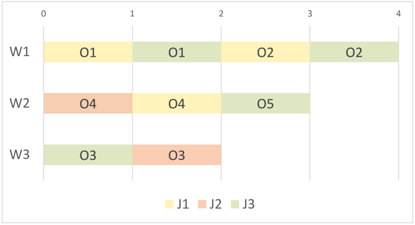
Figure 1: Workers allocations

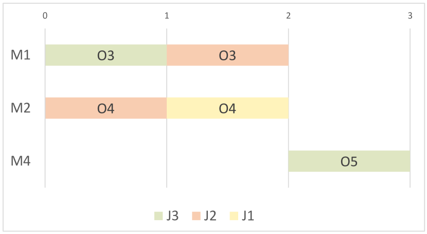
Figure 2: Machines allocations

3.2 Modeling MPF-JSS with Hybrid ASP

Answer Set Programming (ASP) has been widely used in the literature to solve scheduling problems. For instance, in [DBLP:journals/corr/abs-1101-4554] ASP is used to develop a system for computing suitable allocations of personnel on the international seaport of Gioia Tauro. A similar problem of workforce scheduling is also addressed with ASP [DBLP:conf/lpnmr/AbseherGMSW15]. In addition, ASP was applied to solve the course timetabling problem in [DBLP:journals/tplp/BanbaraSTIS13] and [DBLP:conf/padl/KahramanE19]. These approaches, however, indicated one of the major problems of ASP in scheduling applications – grounding issues occurring while dealing with a large number of possible time points. Therefore, in [DBLP:conf/lpnmr/Balduccini11], ASP was integrated with Constraint Programming (CP) techniques to solve the problem of allocating jobs to devices in the context of industrial printing. A different integration of ASP with CP techniques was also suggested in [10.1007/978-3-319-28697-6_23], where two Constraint ASP approaches are proposed to solve a production scheduling problem. In this paper, we use ASP with Difference Logic to model the MPF-JSS problem, which was also applied in [DBLP:conf/lpnmr/AbelsJOSTW19] to schedule railroad traffic.

Problem Instances.

In order to encode the MPF-JSS problem in ASP, we first define a number of predicates representing the input instances. The set of operations is encoded using the predicate op/2 where the first term is indicating the operation identifier, and the second the expected processing times. The demands of operations for resources are described with the needs/2 predicate, see lines 1-3 in Listing 1 encoding the example presented in the previous section.

The set of resources is represented with atoms over the res/3 predicate. An atom res(c,r,o) provides a class c of the required resource, an identifier r of a resource instance, and an operation o it can execute. Thus, the set of required resources can be encoded as shown in lines 5-7.

Finally, the jobs are encoded using three predicates job/2, recipe/2, and prec/3. Atoms over the first predicate provide identifiers of the jobs and their deadlines. Recipes are used to define the set of operations that must be executed for a job, and the partial order of the operations is specified by the atoms over the prec/3 predicate. Respective facts encoding the jobs of our example are given in lines 9-14.

Listing 1: Problem instance

⬇

1op(o1,1). op(o2,1). op(o3,1). op(o4,1). op(o5,1).

2needs(o1,w). needs(o2,w). needs(o3,m). needs(o3,w).

3needs(o4,m). needs(o4,w). needs(o5,m). needs(o5,w).

5res(w,w1,o1). res(w,w1,o2). res(w,w2,o4). res(w,w2,o5).

6res(w,w3,o2). res(w,w3,o3). res(w,w3,o4).

7res(m,m1,o3). res(m,m2,o4). res(m,m3,o4). res(m,m4,o5).

9job(j1,3). job(j2,3). job(j3,3).

10recipe(j1,o1). recipe(j1,o2). recipe(j1,o4).

11recipe(j2,o3). recipe(j2,o4).

12recipe(j3,o1). recipe(j3,o2). recipe(j3,o3). recipe(j3,o5).

13prec(j1,o1,o2). prec(j1,o1,o4).

14prec(j3,o3,o2). prec(j3,o1,o2). prec(j3,o1,o5).

MPF-JSS Encoding.

The problem encoding is split into three parts:

1. base: encodes all the definitions and constraints for the scheduling requirements (Listings 2, 3, and 4);

2. incremental: implements an incremental search strategy as well as weak constraints for the tardiness optimization (Listing 5); and

3. exponential: uses multi-shot solving to find the upper bound on the tardiness for a given instance using exponential search (Listing LABEL:prg:exp).

The first section of the base subprogram, presented in Listing 2, addresses the allocation of resources, expressed by atoms alloc(R,J,O,M), required to execute an operation of a job. Each operation O of a job J requiring a resource of type R should be executed by exactly one instance M of this resource. Since the instances of a resource are equivalent, we introduce a symmetry-breaking constraint in lines 21-15. This constraint avoids unnecessary allocation variants by requiring the solver to select resources starting from the ones with the lexicographically smallest identifier.

Listing 2: Encoding of the resource allocation

⬇

7{alloc(R,J,O,M) : res(R,M,O)}=1 :- recipe(J,O), needs(O,R).

9allocated(R,M) :- alloc(R,J,O,M).

10:- alloc(R,J,O,N), res(R,M,O), M < N, not allocated(R,M).

Listing 3 shows the second part of the base subprogram. The rule in lines 17-18 specifies that the order in which two operations of a job are executed can be arbitrary when these operations are not subject to the job’s precedence relation. Similarly, an arbitrary order is possible if two operations of different jobs require the same resource (lines 33-34). For the operations that need an ordering, expressed by atoms over the ord/4 predicate, we generate an execution sequence – denoted by the seq/4 predicate – using the rules in lines 36 and 39. The sequence of operations whose precedence is given in the input instance is forced by the rule in line LABEL:prg:base:seq:prec.

Listing 3: Encoding of operation sequences

⬇

12{alloc(R,J,O,M) : res(R,M,O)}=1 :- recipe(J,O), needs(O,R).

14allocated(R,M) :- alloc(R,J,O,M).

15:- alloc(R,J,O,N), res(R,M,O), M < N, not allocated(R,M).

17ord(J,O1,J,O2) :- recipe(J,O1), recipe(J,O2), O1 < O2,

18 not prec(J,O1,O2), not prec(J,O2,O1).

19ord(J1,O1,J2,O2) :- alloc(R,J1,O1,M), alloc(R,J2,O2,M),

Listing 4: Difference constraints on operations’ starting times

⬇

21allocated(R,M) :- alloc(R,J,O,M).

Finally, in Listing 4 we introduce the difference constraints encoding the starting times of operations. We represent the starting time of an operation O of job J by an integer variable (J,O). The first constraint in line 41 requires the starting time of each operation to be greater or equal to $0$. The second constraint enforces the starting times to be compatible with the order provided by atoms over the seq/4 predicate. That is, an operation (J2,O2) coming after (J1,O1) must not start before (J1,O1) is finished.

Multi-shot Solving.

Finding solutions of minimal tardiness for MPF-JSS instances can be hard since, without the knowledge of any reasonable bounds on the scheduling time interval, a solver may have to enumerate a large number of possible solutions. Finding such bounds can be complicated and simple heuristics, like determining a maximal sum of operation durations for a particular resource, often provide very imprecise approximations. Therefore, we exploit the power of multi-shot solving to find an upper bound on the tardiness and thus provide a good starting point for the optimization methods of an ASP solver. In the following, we present two approaches to incrementally search for feasible solutions to a given problem instance.

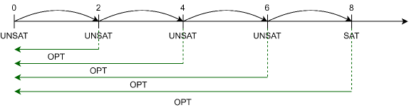
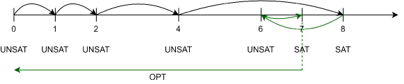
Figure 3: Incremental approach

Figure 4: Exponential approach

The idea of the first approach is to incrementally increase the upper bound on the tardiness of each job in order to identify an interval for which a schedule exists. The algorithm starts by considering the $0$ tardiness bound, and if this yields unsatisfiability (UNSAT), it starts to increment the tardiness bounds by a constant. As a result, the algorithm implements a tumbling window search strategy. The corresponding subprogram step(m,n), shown in Listing 5, takes the parameters m and n to indicate the lower and upper bounds of the interval considered in the current iteration. The parameter values are set via a Python control script, which shifts them by the considered window size in each iteration. The control is implemented using the #external directive, which provides a mechanism to activate or deactivate constraints by assigning a corresponding tardiness(n) atom to true or false, respectively. Figure 4 illustrates a sample execution of the incremental search algorithm, where a tumbling window of size $2$ is moved in each iteration until the target interval for which a schedule exists is found.

Once the admissible upper bound n (and a corresponding lower bound m) is identified, ASP optimization methods search for an optimal solution within this interval, where the truth of an end(J,N) atom for N in-between $1$ and n expresses that the tardiness of job J is less than N. Such atoms can be guessed to be true via the choice rule in line LABEL:prg:step:begin. The constraint in line LABEL:prg:step:tardiness:one propagates smaller tardiness up to the upper bound n, and line LABEL:prg:step:tardiness:two forces the tardiness of each job to be less than n. Finally, we minimize the number of pairs J,N for which end(J,N) is false, i.e., the tardiness of job J is at least N, by means of the weak constraint in line LABEL:prg:step:end. Such an optimization strategy is required since clingo[DL] does not directly allow for minimizing a sum of integer variables occurring in its difference constraints. Therefore, in lines LABEL:prg:step:constraint:begin-LABEL:prg:step:constraint:end, we force each operation of a job to finish within the corresponding tardiness bound. In an obtained answer set, the end(J,N) atom with the smallest value for N signals the tardiness N-1 for job J.

Listing 5: Step subprogram for incremental approach

⬇

33ord(J1,O1,J2,O2) :- alloc(R,J1,O1,M),

34 alloc(R,J2,O2,M), J1 < J2.

36{seq(J1,O1,J2,O2)} :- ord(J1,O1,J2,O2).

37seq(J2,O2,J1,O1) :- ord(J1,O1,J2,O2),

38 not seq(J1,O1,J2,O2).

39seq(J,O1,J,O2) :- prec(J,O1,O2).

41%% start time >= 0

42&diff{0 - (J,O)} <= 0 :- recipe(J,O).

44% do not allow overlapping ops

In the second approach, shown in Listing LABEL:prg:exp, the additional subprogram iterate(n) is used first to find an upper tardiness bound n for each job such that some schedule exists. This is accomplished by a binary search that exponentially increments n until the first schedule is found, and then converges to the smallest n for which the scheduling problem is still satisfiable (SAT). Figure 4 illustrates the process converging to the upper bound $7$, relative to which the tardiness optimization is performed in the second step. In fact, with the iteration(n) atom from the #external directive in line LABEL:prg:iterate:external set to true, the constraint in lines LABEL:prg:iterate:begin-LABEL:prg:iterate:end forces the tardiness of each job to be less than n, and it remains to add the step(1,n-1) subprogram as above for optimization, yet letting the external atom tardiness(n-1) be false to avoid unsatisfiability due to the constraint in line LABEL:prg:step:tardiness:two.