Measuring Dependence with Matrix-based Entropy Functional

Abstract

Measuring the dependence of data plays a central role in statistics and machine learning. In this work, we summarize and generalize the main idea of existing information-theoretic dependence measures into a higher-level perspective by the Shearer’s inequality. Based on our generalization, we then propose two measures, namely the matrix-based normalized total correlation ($T_{\alpha}^{*}$) and the matrix-based normalized dual total correlation ($D_{\alpha}^{*}$), to quantify the dependence of multiple variables in arbitrary dimensional space, without explicit estimation of the underlying data distributions. We show that our measures are differentiable and statistically more powerful than prevalent ones. We also show the impact of our measures in four different machine learning problems, namely the gene regulatory network inference, the robust machine learning under covariate shift and non-Gaussian noises, the subspace outlier detection, and the understanding of the learning dynamics of convolutional neural networks (CNNs), to demonstrate their utilities, advantages, as well as implications to those problems. Code of our dependence measure is available at: https://bit.ly/AAAI-dependence.

Introduction

Measuring the strength of dependence between random variables plays a central role in statistics and machine learning. For the linear dependence case, measures such as the Pearson’s $\rho$, the Spearman’s rank and the Kendall’s $\tau$ are computationally efficient and have been widely used. For the more general case where the two variables share a nonlinear relationship, one of the most well-known dependence measures is the mutual information and its modifications such as the maximal information coefficient (Reshef et al. 2011).

However, real-world data often contains three or more variables which can exhibit higher-order dependencies. If bivariate based measures are used to identify multivariate dependence, wrong conclusions may drawn. For example, in the XOR gate, we have $\mathbf{y}=\mathbf{x}^{1}\oplus\mathbf{x}^{2}$ with $\mathbf{x}^{1}$, $\mathbf{x}^{2}$ being binary random processes with equal probability. Although $\mathbf{x}^{1}$, $\mathbf{x}^{2}$ individually are independent to $\mathbf{y}$, the full dependence is synergistically contained in the union of $\{\mathbf{x}^{1},\mathbf{x}^{2}\}$ and $\mathbf{y}$.

On the other hand, in various practical applications, the observational data or variables of interest lie on a high-dimensional space. Thus, it is desirable to extend the theory of scalar variable dependence to an arbitrary dimension.

Despite that tremendous efforts have been made based on the seven postulates (on measure of dependence on pair of variables) proposed by Alfréd Rényi (Rényi 1959), the problem of measuring dependence (especially in a nonparametric manner) still remains challenging and unsatisfactory (Fernandes and Gloor 2010). This is not hard to understand. Note that, most of the existing measures are defined as some functions of a density. Thus, a prerequisite for them is to estimate the underlying data distributions, a notoriously difficult problem in high-dimensional space.

Moreover, current measures primarily focus on two special scenarios: 1) the dependence associated with each dimension of a random vector (e.g., the multivariate maximal correlation (MAC) (Nguyen et al. 2014)); and 2) the dependence between two random vectors (e.g., the Hilbert Schmidt Independence Criterion (HSIC) (Gretton et al. 2005)). The former is called multivariate correlation analysis in machine learning, and the latter is commonly referred to as random vector association in statistics.

Our main contributions are multi-fold:

• We provide a unified view of existing information-theoretic dependence measures and illustrate their inner connections. We also generalize the main idea of these measures into a higher-level perspective by the Shearer’s inequality (Chung et al. 1986).

• Motivated by our generalization, we suggest two measures, namely the matrix-based normalized total correlation ($T_{\alpha}^{*}$) and the matrix-based normalized dual total correlation ($D_{\alpha}^{*}$), to quantify the dependence of data by making use of the recently proposed matrix-based Rényi’s $\alpha$-entropy functional estimator (Sanchez Giraldo, Rao, and Principe 2014; Yu et al. 2019).

• We show that $T_{\alpha}^{*}$ and $D_{\alpha}^{*}$ enjoy several appealing properties. First, they are not constrained by the number of variables and variable dimension. Second, they are statistically more powerful than most of the prevalent measures. Moreover, they are differentiable, which make them suitable to be used as loss functions to train neural networks.

• We show that our measures offer a remarkable performance gain to benchmark methods in applications like gene regulatory network (GRN) inference and subspace outlier detection. They also provide insights to challenging topics like the understanding of the dynamics of learning of Convolutional Neural Networks (CNNs).

• Motivated by (Greenfeld and Shalit 2020) that training a neural network by encouraging the distribution of the prediction residuals $e$ is statistically independent of the distribution of the input $\mathbf{x}$, we show that our measure (as a loss) improves robust machine learning against the shift of the input distribution ($a.k.a.$, the covariate shift (Sugiyama et al. 2008)) and non-Gaussian noises. We also establish the connection between our loss to the minimum error entropy (MEE) criterion (Erdogmus and Principe 2002), a learning principle that has been extensively investigated in signal processing and process control.

Background Knowledge

Problem Formulation

We consider the problem of estimating the total amount of dependence of the $d_{m}$-dimensional components of the random variable $\mathbf{y}=[\mathbf{y}^{1};\mathbf{y}^{2};\cdots;\mathbf{y}^{L}]\in\mathbb{R}^{d}$, in which the $m$-th component $\mathbf{y}^{m}\in\mathbb{R}^{d_{m}}$ and $d=\sum_{m=1}^{L}d_{m}$. The estimation is based purely on $N$ i.i.d. samples from $\mathbf{y}$, i.e., $\{\mathbf{y}_{i}\}_{i=1}^{N}$. Usually, we expect the derived statistic to be strictly between $0$ and $1$ for improved interpretability (Wang et al. 2017).

Obviously, when $L=2$, we are dealing with random vector association between $\mathbf{y}^{1}\in\mathbb{R}^{d_{1}}$ and $\mathbf{y}^{2}\in\mathbb{R}^{d_{2}}$. Notable measures in this category include the HSIC, the Randomized Dependence Coefficient (RDC) (Lopez-Paz, Hennig, and Schölkopf 2013), the Cauchy-Schwarz quadratic mutual information (QMI_CS) (Principe et al. 2000) and the recently developed mutual information neural estimator (MINE) (Belghazi et al. 2018). On the other hand, in case of $d_{i}=1$ $(i=1,2,\cdots,L)$, the problem reduces to the multivariate correlation analysis on each dimension of $\mathbf{y}$. Examples in this category are the multivariate Spearman’s $\rho$ (Schmid and Schmidt 2007) and the MAC.

Different from the above mentioned measures, we seek a general measure that is applicable to multiple variables in an arbitrary dimensional space (i.e., without constrains on $L$ and $d_{i}$). But, at the same time, we also hope that our measure is interpretable and statistically more powerful than existing counterparts in quantifying either random vector association or multivariate correlation.

A Unified View of Information-Theoretic Measures

From an information-theoretic perspective, a dependence measure $M$ that quantifies how much a random vector $\mathbf{y}=\{\mathbf{y}^{1};\mathbf{y}^{2};\cdots;\mathbf{y}^{L}\}\in\mathbb{R}^{d}$ deviates from statistical independence in each component can take the form of:

$$M(\mathbf{y})=\mathsf{diff}\left(\mathsf{Pr}\left(\mathbf{y}^{1},\mathbf{y}^{2},\cdots,\mathbf{y}^{L}\right):\prod_{i=1}^{L}\mathsf{Pr}\left(\mathbf{y}^{i}\right)\right),$$ (1)

where $\mathsf{diff}$ refers to a measure of difference such as divergence or distance.

If one instantiates $\mathsf{diff}\left(\right)$ with Kullback¨CLeibler (KL) divergence, Eq. (1) reduces to the renowned Total Correlation (Watanabe 1960):

$$T(\mathbf{y}) = D_{\text{KL}}\left(\mathsf{Pr}\left(\mathbf{y}^{1},\mathbf{y}^{2},\cdots,\mathbf{y}^{L}\right)||\prod_{i=1}^{L}\mathsf{Pr}\left(\mathbf{y}^{i}\right)\right),$$ (2)

$$= \left[\sum_{i=1}^{L}{H(\mathbf{y}^{i})}\right]-H(\mathbf{y}^{1},\mathbf{y}^{2},\cdots,\mathbf{y}^{L}),$$

where $H$ denotes entropy or joint entropy.

Most of the existing measures approach multivariate dependence through TC by a decomposition into multiple small variable sets (proof in supplementary material):

$$T(\mathbf{y})=\sum_{i=1}^{L}{H(\mathbf{y}^{i})-H(\mathbf{y}^{i}|\mathbf{y}^{[i-1]})}.$$ (3)

In fact, these measures only vary in the way to estimate $H(\mathbf{y}^{i})$ and $H(\mathbf{y}^{i}|\mathbf{y}^{[i-1]})$. For example, multivariate correlation (Joe 1989) and MAC (Nguyen et al. 2014) use Shannon discrete entropy, whereas CMI (Nguyen et al. 2013) resorts to the cumulative entropy (Rao et al. 2004) which can be directly applied on continuous variables. Although such progressive aggregation strategy helps a measure scales well to high dimensionality, it is sensitive to the ordering of the variables, i.e., Eq. (3) is not permutation invariant. One should note that, there are a total of $L!$ possible permutations, which makes the decomposition scheme always achieve sub-optimal performances.

There are only a few exceptions avoid to the use of TC. A notable one is the Copula-based Kernel Dependence Measures (C-KDM) (Poczos, Ghahramani, and Schneider 2012), which instantiates $\mathsf{diff}\left(\right)$ in Eq. (1) with the Maximum Mean Discrepancy (MMD) (Gretton et al. 2012) and measures the discrepancy between $\mathsf{Pr}\left(\mathbf{y}^{1},\mathbf{y}^{2},\cdots,\mathbf{y}^{L}\right)$ and $\prod_{i=1}^{L}\mathsf{Pr}\left(\mathbf{y}^{i}\right)$ by first taking an empirical copular transform on both distributions. Although C-KDM is theoretically sound and permutation invariant, the value of C-KDM is not upper bounded, which makes it suffer from poor interpretability.

Last and not the least, the above mentioned measures can only deal with scalar variables. Thus, it still remains challenging when each variable is of an arbitrary dimension.

Generalization of TC with Shearer’s Inequality

One should note that, TC is not the only non-negative measures of multivariate dependence. In fact, it can be seen as the simplest member of a large family, all obtained as special cases of an inequality due to Shearer (Chung et al. 1986).

Given a set of $L$ random variables $\mathbf{y}^{1},\mathbf{y}^{2},\cdots,\mathbf{y}^{L}$. Denote $\varphi$ the family of all subsets of $[L]$ with the property that every member of $[L]$ lies in at least $k$ members of $\varphi$, the Shearer’s inequality states that:

$$H(\mathbf{y}^{1},\mathbf{y}^{2},\cdots,\mathbf{y}^{L})\leq\frac{1}{k}\sum_{S\in\varphi}H(\mathbf{y}^{i},i\in S).$$ (4)

Obviously, TC (i.e., Eq. (2)) is obtained when $\varphi={{L}\choose{1}}$.

Another important inequality arises when we take $\varphi={{L}\choose{L-1}}$, in which the Shearer’s inequality suggests an alternative non-negative multivariate dependence measure as:

$$D(\mathbf{y})=\left[\sum_{i=1}^{L}H(\mathbf{y}^{[L]\setminus i})\right]-(L-1)H(\mathbf{y}^{1},\mathbf{y}^{2},\cdots,\mathbf{y}^{d}).$$ (5)

Eq. (5) is also called the dual total correlation (DTC) (Sun 1975) and has an equivalent form (Austin 2018; Abdallah and Plumbley 2012) (see proof in supplementary material):

$$D(\mathbf{y})=H(\mathbf{y}^{1},\mathbf{y}^{2},\cdots,\mathbf{y}^{d})-\left[\sum_{i=1}^{L}H(\mathbf{y}^{i}|\mathbf{y}^{[L]\setminus i})\right].$$ (6)

The Shearer¡¯s inequality suggests the existence of at least $(L-1)$ potential mathematical formulas to quantify the dependence of data, by just taking the gap between the two sides. Although all belong to the same family, these formulas emphasize different parts of the joint distributions and thus cannot be simply replaced by each other (see an illustrate figure in the supplementary material). Finally, one should note that, the Shearer¡¯s inequality is just a loose bound on the sum of partial entropy terms. It has been recently refined further in (Madiman and Tetali 2010). We leave a rigorous treatment to the tighter bound as future work.

Matrix-based Dependence Measure

Our Measures and their Estimation

We exemplify the use of Shearer’s inequality in quantifying data dependence with TC and DTC in this work. First, to make TC and DTC more interpretable, i.e., taking values in the interval of $[0~{}1]$, we normalize both measures as follows:

$$T^{*}(\mathbf{y})=\frac{\left[\sum_{i=1}^{L}{H(\mathbf{y}^{i})}\right]-H(\mathbf{y}^{1},\mathbf{y}^{2},\cdots,\mathbf{y}^{L})}{\left[\sum_{i=1}^{L}{H(\mathbf{y}^{i})}\right]-\max\limits_{i}{H(\mathbf{y}^{i})}},$$ (7)

$$D^{*}(\mathbf{y})=\frac{\left[\sum_{i=1}^{L}H(\mathbf{y}^{[L]\setminus i})\right]-(L-1)H(\mathbf{y}^{1},\mathbf{y}^{2},\cdots,\mathbf{y}^{L})}{H(\mathbf{y}^{1},\mathbf{y}^{2},\cdots,\mathbf{y}^{L})}.$$ (8)

Eqs. (7) and (8) involve entropy estimation in high-dimensional space, which is a notorious problem in statistics and machine learning (Belghazi et al. 2018). Although data discretization or entropy term decomposition has been used before to circumvent the “curse of dimensionality”, they all have their own intrinsic limitations. For data discretization, selecting a proper data discretization strategy is a tricky problem and an improper discretization may lead to serious estimation error. For entropy term decomposition, the resulting measure is no longer permutation invariant.

Different from earlier efforts, we introduce the recent proposed matrix-based Rényi’s $\alpha$-entropy functional (Sanchez Giraldo, Rao, and Principe 2014; Yu et al. 2019), which evaluate entropy terms in terms of the normalized eigenspectrum of the Hermitian matrix of the projected data in the reproducing kernel Hilbert space (RKHS), without explicit evaluation of the underlying data distributions. For brevity, we directly give the following definition.

Definition 1.

(Sanchez Giraldo, Rao, and Principe 2014) Let $\kappa:\mathcal{Y}\times\mathcal{Y}\mapsto\mathbb{R}$ be a real valued positive definite kernel that is also infinitely divisible (Bhatia 2006). Given $Y=\{y_{1},y_{2},\cdots,y_{N}\}$, where the subscript $i$ denotes the exemplar index, and the Gram matrix $K$ obtained from evaluating a positive definite kernel $\kappa$ on all pairs of exemplars, that is $(K)_{ij}=\kappa(y_{i},y_{j})$, a matrix-based analogue to Rényi’s $\alpha$-entropy for a normalized positive definite (NPD) matrix $A$ of size $N\times N$, such that $\mathrm{tr}(A)=1$, can be given by the following functional:

$$\mathbf{S}_{\alpha}(A)=\frac{1}{1-\alpha}\log_{2}\left(\mathrm{tr}(A^{\alpha})\right)=\frac{1}{1-\alpha}\log_{2}\big{[}\sum_{i=1}^{N}\lambda_{i}(A)^{\alpha}\big{]},$$ (9)

where $A_{ij}=\frac{1}{N}\frac{K_{ij}}{\sqrt{K_{ii}K_{jj}}}$ and $\lambda_{i}(A)$ denotes the $i$-th eigenvalue of $A$.

Definition 2.

(Yu et al. 2019) Given a collection of $N$ samples $\{s_{i}=(y_{i}^{1},y_{i}^{2},\cdots,y_{i}^{L})\}_{i=1}^{N}$, each sample contains $L$ ($L\geq 2$) measurements $y^{1}\in\mathcal{Y}^{1}$, $y^{2}\in\mathcal{Y}^{2}$, $\cdots$, $y^{L}\in\mathcal{Y}^{L}$ obtained from the same realization, and the positive definite kernels $\kappa_{1}:\mathcal{Y}^{1}\times\mathcal{Y}^{1}\mapsto\mathbb{R}$, $\kappa_{2}:\mathcal{Y}^{2}\times\mathcal{Y}^{2}\mapsto\mathbb{R}$, $\cdots$, $\kappa_{L}:\mathcal{Y}^{L}\times\mathcal{Y}^{L}\mapsto\mathbb{R}$, a matrix-based analogue to Rényi’s $\alpha$-order joint-entropy among $L$ variables can be defined as:

$$\mathbf{S}_{\alpha}(A^{[L]})=\mathbf{S}_{\alpha}\left(\frac{A^{1}\circ A^{2}\circ\cdots\circ A^{L}}{\mathrm{tr}(A^{1}\circ A^{2}\circ\cdots\circ A^{L})}\right),$$ (10)

where $(A^{1})_{ij}=\kappa_{1}(y_{i}^{1},y_{j}^{1})$, $(A^{2})_{ij}=\kappa_{2}(y_{i}^{2},y_{j}^{2})$, $\cdots$, $(A^{L})_{ij}=\kappa_{L}(y_{i}^{L},y_{j}^{L})$, and $\circ$ denotes the Hadamard product.

Based on the above definition, we propose a pair of measures, namely the matrix-based normalized total correlation (denoted by $T_{\alpha}^{*}$) and the matrix-based normalized dual total correlation (denoted by $D_{\alpha}^{*}$):

$$T_{\alpha}^{*}(\mathbf{y})=\frac{\left[\sum_{i=1}^{L}{S_{\alpha}(A^{i})}\right]-S_{\alpha}\left(A^{[L]}\right)}{\left[\sum_{i=1}^{L}{S_{\alpha}(A^{i})}\right]-\max\limits_{i}S_{\alpha}(A^{i})},$$ (11)

$$D_{\alpha}^{*}(\mathbf{y})=\frac{\left[\sum_{i=1}^{L}S_{\alpha}\left(A^{[L]\setminus i}\right)\right]-(L-1)S_{\alpha}\left(A^{[L]}\right)}{S_{\alpha}\left(A^{[L]}\right)}.$$ (12)

As can be seen, both $T_{\alpha}^{*}$ and $D_{\alpha}^{*}$ are independent of the specific dimensions of $\mathbf{y}^{1},\mathbf{y}^{2},\cdots,\mathbf{y}^{L}$ and avoid estimation of the underlying data distributions, which makes them suitable to be applied on data with either discrete or continuous distributions. Moreover, it is simple to verify that both $T_{\alpha}^{*}$ and $D_{\alpha}^{*}$ are permutation invariant to the ordering of variables.

Properties and Observations of $T_{\alpha}^{*}$ and $D_{\alpha}^{*}$

We present more useful properties and observations of $T_{\alpha}^{*}$ and $D_{\alpha}^{*}$. In particular, we want to underscore that they are differentiable and can be used as loss functions to train neural networks. Note that, when $L=2$, both $T_{\alpha}^{*}$ and $D_{\alpha}^{*}$ reduce to the matrix-based normalized mutual information, which we denote by $I_{\alpha}^{*}$. See the supplementary material for proofs and additional supporting results.

Property 1.

$0\leq T_{\alpha}^{*}\leq 1$ and $0\leq D_{\alpha}^{*}\leq 1$.

Remark.

A major difference between our $T_{\alpha}^{*}$ and $D_{\alpha}^{*}$ to others is that our bounded property is satisfied with a finite number of realizations. An interesting and rather unfortunate fact is that although the statistics of many measures satisfies this desired property, their corresponding estimators hardly follow it (Seth and Príncipe 2012).

Property 2.

$T_{\alpha}^{*}$ and $D_{\alpha}^{*}$ reduce to zero iff $\mathbf{y}^{1},\mathbf{y}^{2},\cdots,\mathbf{y}^{L}$ are independent.

Property 3.

$T_{\alpha}^{*}$ and $D_{\alpha}^{*}$ have analytical gradients and are automatically differentiable.

Remark.

This property complements the theory of the matrix-based Rényi’s $\alpha$-entropy functional (Sanchez Giraldo, Rao, and Principe 2014; Yu et al. 2019), as it opens the door to challenging machine learning problems involving neural networks (as will be illustrated later in this work).

Property 4.

The computational complexity of $T_{\alpha}^{*}$ and $D_{\alpha}^{*}$ are respectively $\mathcal{O}(LN^{2})+\mathcal{O}(N^{3})$ and $\mathcal{O}(LN^{3})$, and grows linearly with the number of variables $L$.

Remark.

In case of $L=2$, both $T_{\alpha}^{*}$ and $D_{\alpha}^{*}$ cost $\mathcal{O}(N^{3})$ in time. As a reference, the computational complexity of HSIC is between $\mathcal{O}(N^{2})$ and $\mathcal{O}(N^{3})$ (Zhang et al. 2018). However, HSIC only applies for two variables and is not upper bounded. We leave reducing the complexity as future work. But the initial exploration results, shown in the supplementary material, suggest that we can reduce the complexity by taking the average of the estimated quantity over multiple random subsamples of size $K\ll N$.

Observation 1.

$T_{\alpha}^{*}$ and $D_{\alpha}^{*}$ are more statistically powerful than prevalent random vector association measures, like HSIC, dCov, KCCA and QMI_CS, in identifying independence and discovering complex patterns between $\mathbf{y}^{1}$ and $\mathbf{y}^{2}$.

We made this observation with the same test data as has been used in (Josse and Holmes 2016; Gretton et al. 2008).

The first test data is generated as follows (Gretton et al. 2008). First, we generate $N$ $i.i.d.$ samples from two randomly picked densities in the ICA benchmark densities (Bach and Jordan 2002). Second, we mixed these random variables using a rotation matrix parameterized by an angle $\theta$, varying from $0$ to $\pi/4$. Third, we added $d-1$ extra dimensional Gaussian noise of zero mean and unit standard deviation to each of the mixtures. Finally, we multiplied each resulting vector by an independent random $d$-dimensional orthogonal matrix. The resulting random vectors are dependent across all observed dimensions.

The second test data is generated as follows (Székely et al. 2007). A matrix $Y^{1}\in\mathbb{R}^{N\times 5}$ is generated from a multivariate Gaussian distribution with an identity covariance matrix. Then, another matrix $Y^{2}\in\mathbb{R}^{N\times 5}$ is generated as $Y_{ml}^{2}=Y_{ml}^{1}\epsilon_{ml}$, $m=1,2,\cdots,N$, $l=1,2,\cdots,5$, where $\epsilon_{ml}$ are standard normal variables and independent of $Y^{1}$.

In each test data, we compare all measures with a threshold computed by sampling a surrogate of the null hypothesis $H_{0}$ based on shuffling samples in $\mathbf{y}^{2}$ with $100$ times. That is, the correspondences between $\mathbf{y}^{1}$ and $\mathbf{y}^{2}$ are broken by the random permutations. The threshold is the estimated quantile $1-\tau$ where $\tau$ is the significance level of the test (Type I error). If the estimated measure is larger than the computed threshold, we reject the null hypothesis and argue the existence of an association between $\mathbf{y}^{1}$ and $\mathbf{y}^{2}$, and vice versa.

We repeated the above procedure $500$ independent trials. Fig. 1 demonstrated the averaged acceptance rate of the null hypothesis $H_{0}$ (in test data I with respect to different rotation angle $\theta$) and the averaged detection rate of the alternative hypothesis $H_{1}$ (in test data II with respect to different number of samples).

Intuitively, in the first test data, a zero angle means the data are independent, while dependence becomes easier to detect as the angle increases to $\pi/4$. Therefore, a desirable measure is expected to have acceptance rate of $H_{0}$ nearly to $1$ at $\theta=0$. But the rate is expected to rapidly decaying as $\theta$ increases. In the second test data, a desirable measure is expected to always have a large detection rate of $H_{1}$ regardless of the number of samples.

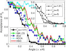
(a) decaying dependence

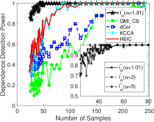
(b) non-monotonic dependence

Figure 1: Power test against prevalent random vector association measures. Our measure is the most powerful one in a large range of $\alpha$.

Observation 2.

$T_{\alpha}^{*}$ and $D_{\alpha}^{*}$ are more interpretable than their multivariate correlation counterparts in quantifying the dependence in each dimension of $\mathbf{y}=\{\mathbf{y}^{1},\mathbf{y}^{2},\cdots,\mathbf{y}^{d}\}\in\mathbb{R}^{d}$.

This observation was made by comparing $T_{\alpha}^{*}$ and $D_{\alpha}^{*}$ against three popular multivariate correlation measures. They are multivariate Spearman’s $\rho$, C-KDM and IDD (Romano et al. 2016). Fig. 2 shows the average value of the analyzed measures on the following relationships induced on $d\in[1,9]$ and $n=1000$ points:

Data A: The first dimension $\mathbf{y}^{1}$ is uniformly distributed in $[0,1]$, and $\mathbf{y}^{i}=(\mathbf{y}^{1})^{i}$ for $i=2,3,\cdots,d$. The total dependence should be $1$, because $\{\mathbf{y}^{2},\mathbf{y}^{3},\cdots,\mathbf{y}^{d}\}$ depend nonlinearly only on $\mathbf{y}^{1}$.

Data B: There is a functional relationship between $\mathbf{y}^{1}$ and the remaining dimensions: $\mathbf{y}^{1}={(\frac{1}{d-1}\sum_{i=2}^{d}\mathbf{y}^{i})}^{2}$, where $\{\mathbf{y}^{2},\mathbf{y}^{3},\cdots,\mathbf{y}^{d}\}$ are uniformly and independently distributed. In this case, the strength of the overall dependence should decrease with the increase of dimension.

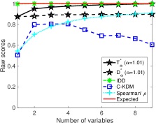
(a) Data A

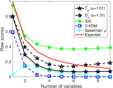
(b) Data B

Figure 2: Raw measure scores on synthetic data with different relationships.

Machine Learning Applications

We present four solid machine learning applications to demonstrate the utility and superiority of our proposed matrix-based normalized total correlation ($T_{\alpha}^{*}$) and matrix-based normalized dual total correlation ($D_{\alpha}^{*}$). The applications include the gene regulatory network (GRN) inference, the robust machine learning under covariate shift and non-Gaussian noises, the subspace outlier detection and the understanding of the dynamics of learning of CNNs. The logic behind the organization of these applications is shown in Table 1. We want to emphasize here that the use of normalization depends on the priority given to interpretability. For example, when the measure is employed as a loss function, the normalization does not contribute to performance. However, when we use it to quantify information flow or neural interactions in CNNs, a bounded value is preferred.

	$d_{i}=1$	$d_{i}\in\mathbb{Z}^{+}$
$L=2$	$\rho$, MIC GRN Inference	HSIC, dCov, QMI_CS Robust ML
$L>2$	C-KDM, IDD Outlier Detection	Understanding CNNs

Table 1: Four dependence scenarios. Popular measures in each scenario and potential applications.

Gene Regulatory Network Inference

Gene expressions form a rich source of data from which to infer GRN, a sparse graph in which the nodes are genes and their regulators, and the edges are regulatory relationship between the nodes. In the first application, we resorted to the DREAM$4$ challenge (Marbach et al. 2012) data set for reconstructing GRN. There are $5$ networks in the insilico (simulated) version of this data set, each contains expressions for $10$ genes with $136$ data points. The goal is to reconstruct the true network based on pairwise dependence between genes. We compared five test statistics (Pearsons¡¯ $\rho$, mutual information with respectively bin estimator and KSG estimator (Kraskov, Stögbauer, and Grassberger 2004), maximal information coefficient (MIC) (Reshef et al. 2011) and $I_{\alpha}^{*}$), and quantitatively evaluate reconstruction qualify by Area Under the ROC curve (AUC). Table 2 clearly indicates our superior performance.

Data Set	$\rho$	MI (bin)	MI (KSG)	MIC	$I_{\alpha}^{*}$
Network $1$	0.62	0.59	0.74	$\underline{0.75}$	$\mathbf{0.78}$
Network $2$	0.52	0.58	$\underline{0.76}$	0.74	$\mathbf{0.87}$
Network $3$	0.44	0.61	$\underline{0.83}$	0.76	$\mathbf{0.84}$
Network $4$	0.45	0.60	$\mathbf{0.75}$	$\mathbf{0.75}$	$\mathbf{0.75}$
Network $5$	0.38	0.61	0.88	$\underline{0.89}$	$\mathbf{0.97}$

Table 2: GRN inference results (AUC score) on DREAM$4$ challenge. The first and second best performances are in bold and underlined, respectively.

Robust Machine Learning

Robust machine learning under domain shift (Quionero-Candela et al. 2009) has attracted increasing attentions in recent years. This is justified because the success of deep learning models is highly dependent on the assumption that the training and testing data are i.i.d. and sampled from the same distribution. Unfortunately, the data in reality is typically collected from different but related domains (Wilson and Cook 2020), and is corrupted (Chen et al. 2016b).

Let $(\mathbf{x},y)$ be a pair of random variables with $\mathbf{x}\in\mathbb{R}^{p}$ and $y\in\mathbb{R}$ (in regression) or $\mathbf{y}\in\mathbb{R}^{q}$ (in classification), such that $\mathbf{x}$ denotes input instance and $y$ denotes desired signal. We assume $\mathbf{x}$ and $y$ follow a joint distribution $P_{\text{source}}(\mathbf{x},y)$. Our goal is, given training samples drawn from $P_{\text{source}}(\mathbf{x},y)$, to learn a model $f$ predicting $y$ from $\mathbf{x}$ that works well on a different, a-priori unknown target distribution $P_{\text{target}}(\mathbf{x},y)$. We consider here only the covariate shift, in which the assumption is that the conditional label distribution is invariant (i.e., $P_{\text{target}}(y|\mathbf{x})=P_{\text{source}}(y|\mathbf{x})$) but the marginal distributions of input $P(\mathbf{x})$ are different between source and target domains (i.e., $P_{\text{target}}(\mathbf{x})\neq\ P_{\text{source}}(\mathbf{x})$). On the other hand, we also assume that $y$ (in the source domain) may be contaminated with non-Gaussian noises (i.e., $\widetilde{y}=y+\epsilon$). We focus on a fully unsupervised environment, in which we have no access to any samples $\mathbf{x}$ or $y$ from the target domain, i.e., the source-to-target manifold alignment becomes burdensome.

Our work in this section is directly motivated by (Greenfeld and Shalit 2020), which introduces the criterion of minimizing the dependence between input $\mathbf{x}$ and prediction error $e=y-f(\mathbf{x})$ to circumvent the covariate shift, and uses the HSIC as the measure to quantify the independence. We provide two contributions over (Greenfeld and Shalit 2020). In terms of methodology, we show that by replacing HSIC with our new measures (i.e., $I_{\alpha}^{*}$), we improve the prediction accuracy in the target domain. Theoretically, we show that our new loss, namely $\min I_{\alpha}^{*}(\mathbf{x};e)$ is not only robust against covariate shift and also non-Gaussian noises on $y$ based on Theorem 1.

Theorem 1.

Minimizing the (normalized) mutual information $I(\mathbf{x};e)$ is equivalent to minimizing error entropy $H(e)$.

Remark.

The minimum error entropy (MEE) criterion (Erdogmus and Principe 2002) has been extensively studied in signal processing to address non-Gaussian noises with both theoretical guarantee and empirical evidence (Chen et al. 2009, 2016a). We summarize in supplementary material two insights to further clarify its advantage.

Learning under covariate shift.

We first compare the performances of cross entropy (CE) loss, HSIC loss with our error entropy $H_{\alpha}(e)$ loss and $I_{\alpha}^{*}(\mathbf{x};e)$ loss under covariate shift. Following (Greenfeld and Shalit 2020), the source data is the Fashion-MNIST dataset (Xiao, Rasul, and Vollgraf 2017), and images which are rotated by an angle $\theta$ sampled from a uniform distribution over $[-20\degree,20\degree]$ constitute the target data. The neural network architecture is set as: there are $2$ convolutional layers (with, respectively, $16$ and $32$ filters of size $5\times 5$) and $1$ fully connected layers. We add batch normalization and max-pooling layer after each convolutional layer. We choose ReLU activation, batch size $128$ and the Adam optimizer (Kingma and Ba 2014).

For $I_{\alpha}^{*}(\mathbf{x};e)$ and $H_{\alpha}(e)$, we set $\alpha=2$. For the HSIC loss, we take the same hyper-parameters as in (Greenfeld and Shalit 2020). The results are summarized in Table 3. Our $H_{\alpha}(e)$ performs comparably to HSIC, but our $I_{\alpha}(\mathbf{x};e)$ improves performances in both source and target domains.

Method	Fashion MNIST
	Source	Target
CE	$90.90\pm 0.002$	$73.73\pm 0.086$
HSIC	$91.03\pm 0.003$	$76.56\pm 0.034$
$H_{\alpha}(e)$	$91.10\pm 0.013$	$75.48\pm 0.069$
$I_{\alpha}^{*}(\mathbf{x};e)$	$\mathbf{91.17\pm 0.040}$	$\mathbf{76.79\pm 0.040}$

Table 3: Test accuracy (%) on Fashion-MNIST

Learning in noisy environment.

We select the widely used bike sharing data set (Fanaee-T and Gama 2014) in UCI repository, in which the task is to predict the number of hourly bike rentals based on the following features: holiday, weekday, workingday, weathersit, temperature, feeling temperature, wind speed and humidity. Consisting of $17,379$ samples, the data was collected over two years, and can be partitioned by year and season. Early studies suggest that this data set contains covariate shift due to the change of time (Subbaswamy, Schulam, and Saria 2019).

We use the first three seasons samples as source data and the forth season samples as target data. The model of choice is a multi-layered perceptron (MLP) with three hidden layer of size 100, 100 and 10 respectively. We compare our $I_{\alpha}^{*}(\mathbf{x};e)$ and $H_{\alpha}(e)$ with mean square error (MSE), mean absolutely error (MAE) and HSIC loss, assuming $y$ is contaminated with additive noise as $\widetilde{y}=y+\epsilon$. We consider two common non-Gaussian noises with the noise level controlled by parameter $\rho$: the Laplace noise $\epsilon\sim\textmd{Laplace}(0,\rho)$; and the shifted exponential noise $\epsilon=\rho(1-\eta)$ with $\eta\sim\textmd{exp}(1)$. We use batch-size of $32$ and the Adam optimizer.

We compared our $I_{\alpha}^{*}(\mathbf{x};e)$ and $H_{\alpha}(e)$ against MSE loss, MAE loss and HSIC loss. Fig. 3 demonstrates the averaged performance gain (or loss) of different loss functions over MSE loss in $10$ independent runs. In most of cases, $I_{\alpha}^{*}(\mathbf{x};e)$ improves the most. HSIC is not robust to Laplacian noise, whereas MAE performs poorly under shifted exponential noise. On the other hand, $H_{\alpha}(e)$ also obtained a consistent performance gain over MSE, which further corroborates our theoretical arguments.

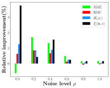
(a) Laplacian

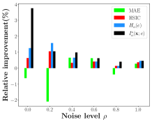
(b) Shifted exponential

Figure 3: Comparisons of models trained with MSE, MAE, HSIC loss, $I_{\alpha}^{*}(\mathbf{x};e)$ and $H_{\alpha}(e)$. Each bar denotes the relative performance gain (or loss) over MSE.

Subspace Outlier Detection

Our third application is the outlier detection, in which we aim to identify data objects that do not fit well with the general data distributions (in $\mathbb{R}^{d}$). Despite diverse paradigms, such as the density-based methods (Breunig et al. 2000) and the distance-based methods (Bay and Schwabacher 2003), have been developed so far, they usually suffer from the notorious “curse of dimensionality” (Keller, Muller, and Bohm 2012). In fact, the principle of concentration of distance (Beyer et al. 1999) reveals that for a query point $p$, its relative distance (or contrast) $D$ to the farthest point and the nearest point converges to $0$ with the increase of dimensionality $d$:

$$\lim_{d\rightarrow\infty}{\frac{D_{max}-D_{min}}{D_{min}}}\rightarrow 0.$$ (13)

This means that the discriminative power between the nearest and the farthest neighbor becomes rather poor in high-dimensional space.

On the other hand, real data often contains irrelevant attributes or noises. This phenomenon degrades further the performance of most existing outlier detection methods if the outliers are hidden in subspaces of all given attributes (Kriegel, Schubert, and Zimek 2008). Therefore, the subspace methods that explore lower-dimensional subspace in order to discover outliers provide a promising avenue.

Empirical evidence suggests that, the larger the deviation of this subspace from the mutual independence in each dimension, the higher the potential that it is easier to distinguish outliers from normal observations (Müller et al. 2009). Therefore, measuring the total amount of dependence of a subspace becomes a pivotal aspect. To this end, we plug our dependence measure (either $T_{\alpha}^{*}$ or $D_{\alpha}^{*}$) into a commonly used Apriori subspace search scheme (Nguyen et al. 2013) to assess the quality of each subspaces (the larger the better). Next, we detect outliers with a widely-used Local Outlier Factor (LOF) method (Breunig et al. 2000) on the top $10$ subspaces with highest dependence score.

We use again the AUC to quantitatively evaluate outlier detection results of our method against three competitors: 1) LOF in full-space; 2) Feature Bagging (FB) (Lazarevic and Kumar 2005) that applies LOF on randomly selected subspaces; and 3) LOF on subspaces generated by IDD. We omit the results of LOF on the subspaces generated by C-KDM due to relatively poor performance. We test on $5$ publicly available data sets from the Outlier Detection DataSets (ODDS) library (Rayana 2016). These data cover a wide range of number of samples ($N$) and data dimensionality ($d$). The prevalence of anomalies ranges from $1.65\%$ (in speech) to $35\%$ (in breastW). The results are reported in Table 4. As can be seen, our $T_{\alpha}^{*}$ and $D_{\alpha}^{*}$ achieve remarkable performance gain over LOF on all attributes, especially when the $d$ is large. Under a Wilcoxon signed rank test (Demšar 2006) with $0.05$ significance level, both $T_{\alpha}^{*}$ and $D_{\alpha}^{*}$ significantly outperform LOF. This observation corroborates our motivation of reliable subspace search. By contrast, the random subspace selection scheme in FB does not show obvious advantage, and the subspace quality generated by IDD is lower than ours.

Data Set ($N\times d$)	LOF	FB	IDD	$T_{\alpha}^{*}$	$D_{\alpha}^{*}$
Diabetes ($568\times 8$)	$\mathbf{0.68}$	0.63	0.55	$\mathbf{0.68}$	$\mathbf{0.68}$
breastW ($683\times 9$)	0.46	0.53	$\mathbf{0.76}$	$\underline{0.71}$	$\underline{0.71}$
Cardio ($1831\times 21$)	0.68	0.65	0.62	$\mathbf{0.75}$	$\underline{0.70}$
Musk ($3062\times 166$)	0.42	0.40	0.67	$\underline{0.73}$	$\mathbf{0.83}$
Speech ($3686\times 400$)	0.36	0.38	0.50	$\mathbf{0.58}$	$\underline{0.54}$

Table 4: Outlier detection results (AUC score) on real data. The first and second best performances are in bold and underlined, respectively.

Understanding the Dynamics of Learning of CNNs

Understanding the dynamics of learning of deep neural networks (especially CNNs) has received increasing attention in recent years (Shwartz-Ziv and Tishby 2017; Saxe et al. 2018). From an information-theoretic perspective, most studies aim to unveil fundamental properties associated with the dynamics of learning of CNNs by monitoring the mutual information between pairwise layers across training epochs (Yu et al. 2020).

Different from the layer-level dependence, we provide here an alternative way to quantitatively analyze the dynamics of learning in a feature-level. Specifically, suppose there are $N_{t}$ feature maps in the $t$-th convolutional layer. Let us denote them by $C^{1},C^{2},\cdots,C^{N_{t}}$. We use two quantities to capture the dependence in feature maps: 1) the pairwise dependence between the $i$-th feature map and the $j$-th feature map (i.e., $I_{\alpha}^{*}(C^{i};C^{j})$); 2) the total dependence among all feature maps (i.e., $T_{\alpha}^{*}(C^{1},C^{2},\cdots,C^{N_{t}})$).

We train a standard VGG-$16$ (Simonyan and Zisserman 2015a) on CIFAR-$10$ (Krizhevsky 2009) with SGD optimizer from scratch. The $T_{\alpha}^{*}$ in different layers across different training epochs is illustrated in Fig. 4. There is an obvious increasing trend for $T_{\alpha}^{*}$ in all layers during the training, i.e., the total amount of dependence amongst all feature maps continuously increases as the training moves on, until approaching to the value of nearly $1$. A similar observation is also made by HSIC. Note that, the co-adaptation phenomenon has also been observed in fully connected layers and eventually inspired the Dropout (Hinton et al. 2012).

Fig. 5 shows the histogram of $I_{\alpha}^{*}$ in each layer. Similar to the general trend of $T_{\alpha}^{*}$, we observed that the most frequent values of $I_{\alpha}^{*}$ change from nearly $0$ to nearly $1$. Moreover, such movement in lower layers occurs much earlier than that in upper layers. This behavior is in line with (Raghu et al. 2017), which states that the neural networks first train and stabilize lower layers and then move to upper layers.

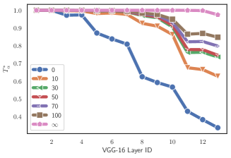
Figure 4: $T_{\alpha}^{*}$ across training epochs for different convolutional layers.

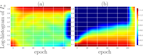
Figure 5: The histogram of $I_{\alpha}^{*}$ (in log-scale) in (a) averaged from the $1$st to the $7$th CONV layers; and (b) averaged from the $8$th to $13$th CONV layer. Feature maps reach high dependence with less than $20$ epochs of training in lower layers, but need more than $100$ epochs in upper layers.

Conclusion

We suggest two measures to quantify from data the dependence of multiple variables with arbitrary dimensions. Distinct from previous efforts, our measures avoid the estimation of the data distributions and are applicable to all dependence scenarios (for i.i.d. data). The proposed measures more easily (e.g., with less data) identify independence and discover complex dependence patterns. Moreover, the differentiable property enables us to design new loss functions for training neural networks.

In terms of specific applications, we demonstrated that the new loss $\min I_{\alpha}^{*}(\mathbf{x};e)$ is robust against both covariate shift and non-Gaussian noises. We also provided an alternative way to analyze the dynamics of learning of CNNs based on the dependence amongst feature maps, and obtained meaningful observations.

In the future, we will explore other properties of our measures. We are interested in applying them to other challenging problems, such as disentangled representation learning with variational autoencoders (VAEs) (Kingma and Welling 2014). We also performed a preliminary investigation on a new robust loss, termed the deep deterministic information bottleneck (DIB), in the supplementary material.

Appendix A Additional Note on $L=2$

When $L=2$ (i.e., only two random variables), both total correlation (TC) and dual total correlation (DTC) reduce to the mutual information $I$:

$$T(\mathbf{y})=D(\mathbf{y})=I(\mathbf{y})=H(\mathbf{y}^{1})+H(\mathbf{y}^{2})-H(\mathbf{y}^{1},\mathbf{y}^{2}),$$ (14)

One can normalize mutual information with either:

$$I^{*}(\mathbf{y})=\frac{H(\mathbf{y}^{1})+H(\mathbf{y}^{2})-H(\mathbf{y}^{1},\mathbf{y}^{2})}{\min\limits_{i}{H(\mathbf{y}^{i})}},$$ (15)

or

$$I^{*}(\mathbf{y})=\frac{H(\mathbf{y}^{1})+H(\mathbf{y}^{2})-H(\mathbf{y}^{1},\mathbf{y}^{2})}{\max\limits_{i}{H(\mathbf{y}^{i})}},$$ (16)

In practice, we observed Eq. (16) always performs better.

Appendix B TC and DTC in Venn Diagram

Although both total correaltion (TC) and dual total correaltion (DTC) reduce to zero in case of pairwise independence, they emphasize different parts of data distribution. When using a Venn diagram to represent a set of four variables $\mathbf{y}^{1},\mathbf{y}^{2},\mathbf{y}^{3},\mathbf{y}^{4}$ as shown in Fig. 6, it is easy to find that TC gives more weights to higher-order interactions (see the dense block areas).

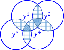
(a) TC or $T_{\alpha}^{*}$

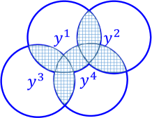
(b) DTC or $D_{\alpha}^{*}$

Figure 6: Illustration of TC (or $T_{\alpha}^{*}$) as compared with DTC (or $D_{\alpha}^{*}$) on a set of four random variables $\mathbf{y}^{1},\mathbf{y}^{2},\mathbf{y}^{3},\mathbf{y}^{4}$. In each case, the quantity is represented by the total amount of block areas of the diagram. TC counts the triple-overlapped areas twice each, whereas DTC counts each overlapped areas just once.

Appendix C Proofs to Eqs. (3) and (6) of the Main Paper

Decomposition of Total Correlation

By definition, we have:

$$T(\mathbf{y})=\left[\sum_{i=1}^{L}{H(\mathbf{y}^{i})}\right]-H(\mathbf{y}^{1},\mathbf{y}^{2},\cdots,\mathbf{y}^{L}),$$ (17)

Eq. (17) is equivalent to:

$$T(\mathbf{y})=\sum_{i=1}^{L}{H(\mathbf{y}^{i})-H(\mathbf{y}^{i}|\mathbf{y}^{[i-1]})}.$$ (18)

Proof.

By the chain rule of joint entropy (Cover 1999), we have:

$$H(\mathbf{y}^{1},\mathbf{y}^{2},\cdots,\mathbf{y}^{L})=\sum_{i=1}^{L}H(\mathbf{y}^{i}|\mathbf{y}^{[i-1]}).$$ (19)

Inserting Eq. (19) into Eq. (17), we get Eq. (18). ∎

Equivalent Expression of Dual Total Correlation

By definition, we have:

$$D(\mathbf{y})=\left[\sum_{i=1}^{L}H(\mathbf{y}^{[L]\setminus i})\right]-(L-1)H(\mathbf{y}^{1},\mathbf{y}^{2},\cdots,\mathbf{y}^{L}).$$ (20)

Eq. (20) is equivalent to:

$$D(\mathbf{y})=H(\mathbf{y}^{1},\mathbf{y}^{2},\cdots,\mathbf{y}^{d})-\left[\sum_{i=1}^{L}H(\mathbf{y}^{i}|\mathbf{y}^{[L]\setminus i})\right].$$ (21)

Proof.

$$D(\mathbf{y}) = \left[\sum_{i=1}^{L}H(\mathbf{y}^{[L]\setminus i})\right]-(L-1)H(\mathbf{y}^{1},\mathbf{y}^{2},\cdots,\mathbf{y}^{L}),$$ (22)

$$= H(\mathbf{y}^{1},\mathbf{y}^{2},\cdots,\mathbf{y}^{L})$$

$$- \sum_{i=1}^{L}\left[H(\mathbf{y}^{1},\mathbf{y}^{2},\cdots,\mathbf{y}^{L})-H(\mathbf{y}^{[L]\setminus i})\right],$$

$$= H(\mathbf{y}^{1},\mathbf{y}^{2},\cdots,\mathbf{y}^{L})-\left[\sum_{i=1}^{L}H(\mathbf{y}^{i}|\mathbf{y}^{[L]\setminus i})\right].$$

∎

Appendix D Proofs and Additional Remarks to Properties

Elaboration of Property 1 and Property 2

Property 5.

$0\leq T_{\alpha}^{*}\leq 1$ and $0\leq D_{\alpha}^{*}\leq 1$.

Proof.

By Corollary 2 in (Yu et al. 2019), we have:

$$S_{\alpha}(A^{[L]})\leq\sum_{i=1}^{L}{S_{\alpha}(A^{i})},$$ (23)

and

$$S_{\alpha}(A^{[L]})\geq\max\limits_{i}S_{\alpha}(A^{i}).$$ (24)

Eqs. (23) and (24) imply $0\leq T_{\alpha}^{*}\leq 1$.

On the other hand, by Corollary 1 also in (Yu et al. 2019), we have:

$$\forall i,S_{\alpha}(A^{[L]})\geq\max\left[S_{\alpha}(A^{i}),S_{\alpha}(A^{[L]\setminus i})\right],$$ (25)

which implies:

$$\forall i,S_{\alpha}(A^{[L]})\geq S_{\alpha}(A^{[L]\setminus i}).$$ (26)

Sum all $L$ inequalities, we obtain:

$$LS_{\alpha}(A^{[L]})\geq\sum_{i=1}^{L}S_{\alpha}(A^{[L]\setminus i}),$$ (27)

which further implies that:

$$\sum_{i=1}^{L}S_{\alpha}(A^{[L]\setminus i})-(L-1)S_{\alpha}(A^{[L]})\leq S_{\alpha}(A^{[L]})$$ (28)

Therefore,

$$D_{\alpha}^{*}(\mathbf{y})=\frac{\left[\sum_{i=1}^{L}S_{\alpha}\left(A^{[L]\setminus i}\right)\right]-(L-1)S_{\alpha}\left(A^{[L]}\right)}{S_{\alpha}\left(A^{[L]}\right)}\leq 1.$$ (29)

The non-negative of $D_{\alpha}^{*}$ or its numerator $D_{\alpha}$ is straightforward, in which we simply use the Lemma 1 (shown in property 2):

$$D_{\alpha}\geq\max\limits_{i}I_{\alpha}(A^{i};A^{[L]\setminus i})\geq 0.$$ (30)

∎

Property 6.

$T_{\alpha}^{*}$ and $D_{\alpha}^{*}$ reduce to zero iff $\mathbf{y}^{1},\mathbf{y}^{2},\cdots,\mathbf{y}^{L}$ are independent.

Because the denominator of $T_{\alpha}^{*}$ and $D_{\alpha}^{*}$ is always larger than $0$, we focus our analysis on the numerator, i.e., the standard total correlation and dual total correlation. Our proof is based on the following lemma.

Lemma 2.

$T(\mathbf{y})$ and $D(\mathbf{y})$ are greater than or equal to $\max\limits_{i}I(\mathbf{y}^{i};\mathbf{y}^{[L]\setminus i})$.

Proof.

For $T(\mathbf{y})$, we have (based on Eq. (18)):

$$T(\mathbf{y}) = \sum_{i=1}^{L}{H(\mathbf{y}^{i})-H(\mathbf{y}^{i}|\mathbf{y}^{[i-1]})}$$ (31)

$$\geq H(\mathbf{y}^{L})-H(\mathbf{y}^{L}|\mathbf{y}^{[L-1]})$$

$$= I(\mathbf{y}^{L};\mathbf{y}^{[L]\setminus L}),$$

in which the second line is based on the fact that $\forall{i},H(\mathbf{y}^{i})\geq H(\mathbf{y}^{i}|\mathbf{y}^{[i-1]})$ and we just take $i=L$.

For $D(\mathbf{y})$, we have (based on Eqs. (19) and (21)):

$$D(\mathbf{y}) = \sum_{i=1}^{L}H(\mathbf{y}^{i}|\mathbf{y}^{[i-1]})-\sum_{i=1}^{L}H(\mathbf{y}^{i}|\mathbf{y}^{[L]\setminus i})$$ (32)

$$= \sum_{i=1}^{L}H(\mathbf{y}^{i}|\mathbf{y}^{[i-1]})-H(\mathbf{y}^{i}|\mathbf{y}^{[L]\setminus i})$$

$$= \sum_{i=1}^{L}I(\mathbf{y}^{i};\mathbf{y}^{i+1,\cdots,L}|\mathbf{y}^{[i-1]})$$

$$\geq I(\mathbf{y}^{1};\mathbf{y}^{[L]\setminus 1}).$$

in which the second line is based on the fact that $\forall{i},I(\mathbf{y}^{i};\mathbf{y}^{i+1,\cdots,L}|\mathbf{y}^{[i-1]})\geq 0$ and we just take $i=1$.

Note that Eqs. (31) and (32) can be applied for any re-ordering of the random variables $\mathbf{y}^{1},\mathbf{y}^{2},\cdots,\mathbf{y}^{L}$, i.e., invariant to the order of $1,2,\cdots,L$. This implies the common lower bound $\max\limits_{i}I(\mathbf{y}^{i};\mathbf{y}^{[L]\setminus i})$. ∎

Note that, mutual information is non-negative. According to Lemma 1, in case of $T(\mathbf{y})=0$ or $D(\mathbf{y})=0$, we have $\forall{i},I(\mathbf{y}^{i};\mathbf{y}^{[L]\setminus i})=0$, which implies that for all $i$, $\mathbf{y}^{i}$ is independent of all rest variables $\mathbf{y}^{1},\cdots,\mathbf{y}^{i-1},\mathbf{y}^{i+1},\cdots,\mathbf{y}^{L}$. Therefore, $T(\mathbf{y})$ and $D(\mathbf{y})$ reduce to zero iff $\mathbf{y}^{1},\mathbf{y}^{2},\cdots,\mathbf{y}^{L}$ are independent.

Elaboration of Property 3

Property 7.

$T_{\alpha}^{*}$ and $D_{\alpha}^{*}$ have analytical gradients and are automatically differentiable.

Mutual information

We focus our analysis on the proposed loss $\min I_{\alpha}(\mathbf{x};e)$, i.e., encouraging the distribution of the prediction residuals $e=y-f_{\theta}(\mathbf{x})$ is statistically independent of the distribution of the input $\mathbf{x}$. Mutual information can be equivalently expressed as the sum of each entropy term minus the joint entropy, i.e., $I_{\alpha}(A;B)=S_{\alpha}(A)+S_{\alpha}(B)-S_{\alpha}(A,B)$, in which $A\in\mathbb{R}^{N\times N}$ and $B\in\mathbb{R}^{N\times N}$ denote two sample Gram matrices generated from $\{\mathbf{x}_{i}\}_{i=1}^{N}$ and $\{e_{i}\}_{i=1}^{N}$, respectively.

According to Definition 1 and Definition 2, we have:

$$S_{\alpha}(A)=\frac{1}{1-\alpha}\log_{2}\left(\mathrm{tr}(A^{\alpha})\right),$$ (33)

and

$$S_{\alpha}(A,B)=S_{\alpha}\left(\frac{A\circ B}{\mathrm{tr}(A\circ B)}\right).$$ (34)

We thus have:

$$\frac{\partial S_{\alpha}(A)}{\partial A}=\frac{\alpha}{(1-\alpha)}\frac{A^{\alpha-1}}{\mathrm{tr}\left(A^{\alpha}\right)},$$ (35)

$$\frac{\partial S_{\alpha}(A,B)}{\partial A}=\frac{\alpha}{(1-\alpha)}\left[\frac{(A\circ B)^{\alpha-1}\circ B}{\mathrm{tr}(A\circ B)^{\alpha}}-\frac{I\circ B}{\mathrm{tr}(A\circ B)}\right],$$ (36)

and

$$\frac{\partial I_{\alpha}(A;B)}{\partial A}=\frac{\partial S_{\alpha}(A)}{\partial A}+\frac{\partial S_{\alpha}(A,B)}{\partial A}.$$ (37)

Since $I_{\alpha}(A;B)$ is symmetric, the same applies for $\frac{\partial I_{\alpha}(A;B)}{\partial B}$ with exchanged roles between $A$ and $B$.

Automatic differentiation

In practice, taking the gradient of the $I_{\alpha}(A,B)$ is simple with any automatic differentiation software, like PyTorch (Paszke et al. 2019) or Tensorflow (Abadi et al. 2016). We use PyTorch in this work, because the obtained gradient is consistent with the analytical one. For example, by the Theorem 1 in (Magnus 1985), the analytical gradient of the $i$-th eigenvalue with respect to a real symmetric matrix $A$ is the outer product of the $i$-th eigenvector ($v_{i}$), i.e.,:

$$\frac{\partial\lambda_{i}}{\partial A}=v_{i}v_{i}^{T}.$$ (38)

We noticed that, with Tensorflow, the diagonal entries are the same to their corresponding analytical values, but the off-diagonal entries are just half.

Elaboration of Property 4

Property 8.

The computational complexity of $T_{\alpha}^{*}$ and $D_{\alpha}^{*}$ are respectively $\mathcal{O}(LN^{2})+\mathcal{O}(N^{3})$ and $\mathcal{O}(LN^{3})$, and grows linearly with the number of variables $L$.

Proof.

For $T_{\alpha}^{*}$, the first term is the complexity of computing $L$ Gram matrices with $N$ samples, while the second term is due to the eigenvalue decomposition of matrices of size $N\times N$.

Similarly, for $D_{\alpha}^{*}$, the main complexity comes from eigenvalue decomposition of $2L$ matrices of size $N\times N$. ∎

In practice, one is able to reduce the complexity by taking the average of the estimated quantity over multiple random subsamples of size $K\ll N$. Suppose we take $M$ groups of subsamples, then the total complexity reduces to $\mathcal{O}(LMK^{2})+\mathcal{O}(MK^{3})$ for $T_{\alpha}^{*}$ and $\mathcal{O}(LMK^{3})$ for $D_{\alpha}^{*}$. Note that, this strategy is common in information-theoretic quantities estimation (Wang and Ding 2019; Ver Steeg 2014) and our initial results (see Figs. 7 and 8) suggest that the power and the interpretability of our measures do not suffer too much with this strategy.

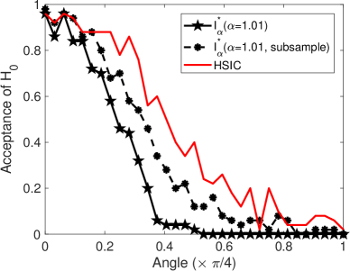
Figure 7: Power test against HSIC in “decaying dependence” data. $I_{\alpha}^{*}$ is obtained with $512$ samples, $I_{\alpha}^{*}$ (subsample) is obtained by taking the average of $10$ groups of subsamples of size $128$. Note that, although the dependence detection power of $I_{\alpha}^{*}$ decreases with subsampling, it is still superior to the established HSIC (with full samples).

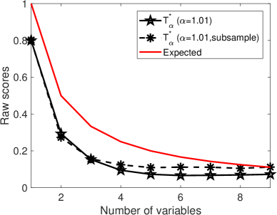
Figure 8: Raw measure scores on Data B. $T_{\alpha}^{*}$ is obtained with $1000$ samples, $T_{\alpha}^{*}$ (subsample) is obtained by taking the average of $10$ groups of subsamples of size $100$. In both cases, the raw scores of $T_{\alpha}^{*}$ have similar values and fit well with the expected ones.

Appendix E Proofs and Additional Remarks to Theorems

Proof of Theorem 1 of the Main Paper

Here we prove the equivalence of $\min I(\mathbf{x};e)$ and $\min H(e)$, where the latter is the well-known minimum error entropy (MEE) criterion (Erdogmus and Principe 2002) that has been extensively investigated in signal processing and process control.

Theorem 3.

Minimizing the mutual information $I(\mathbf{x};e)$ is equivalent to minimizing error entropy $H(e)$.

Proof.

We have:

$$\begin{split}I(\mathbf{x};e)&=H(e)-H(e|\mathbf{x})\\ &=H(e)-H(e+f_{\theta}(\mathbf{x})|\mathbf{x})\\ &=H(e)-H(y|\mathbf{x}),\end{split}$$ (39)

in which the second line is by the property that given two random variables $\xi$ and $\eta$, then for any measurable function $h$, we have $H(\xi|\eta)=H(\xi+h(\eta)|\eta)$. Interested readers can refer to (Cover 1999; MacKay 2003) for a detailed account of this property and its interpretation.

Therefore, $\min I(\mathbf{x};e)$ is equivalent to $\min H(e)$. This is simply by the fact that the conditional entropy of $y$ given $\mathbf{x}$, i.e., $H(y|\mathbf{x})$, is a constant that is purely determined by the training data (regardless of training algorithms). Note that, similar argument has also been claimed in stochastic process control (Feng, Loparo, and Fang 1997). ∎

Insights into $\min H(e)$ against non-Gaussian Noises

We then present two insights on the robustness of $\min H(e)$ over the mean square error (MSE) criterion $\min E(e^{2})$ against non-Gaussian noises, in which $E$ denotes the expectation. Interested readers can refer to (Chen et al. 2009, 2010, 2016a; Hu et al. 2013) for more thorough analysis on the advantage of $\min H(e)$.

First, (Chen et al. 2009, Theorem 3) suggests that $\min E(e^{2})$ is equivalent to minimizing the error entropy plus a Kullback¨CLeibler (KL) divergence. Specifically, we have:

$$\min E(e^{2})\Leftrightarrow\min H(e)+D_{\text{KL}}(p(e)\|\varphi(e)),$$ (40)

in which $p(e)$ is the probability of error, $\varphi(e)$ denotes a zero-mean Gaussian distribution. As the KL-divergence is always nonnegative, minimizing the MSE is equivalent to minimizing an upper bound of the error entropy. Eq. (40) also explains (partially) why in linear and Gaussian cases, the MSE and MEE are equivalent (Kalata and Priemer 1979). Nevertheless, in case the error or noise follows a highly non-Gaussian distribution (especially when the signal-to-noise (SNR) value decreases), the MSE solution deviates from the MEE result, but the latter takes full advantage of high-order information of the error (Chen et al. 2016a).

On the other hand, given the mean-square error $E(e^{2})$, the error entropy satisfies (Cover 1999):

$$H(e)\leq\max_{E(\zeta^{2})=E(e^{2})}H(\zeta)=\frac{1}{2}+\frac{1}{2}\log{2\pi}+\frac{1}{2}\log{(E(e^{2}))},$$ (41)

where $\zeta$ denotes a random variable whose second moment equals to $E(e^{2})$. This implies that the MSE criterion can be recognized as a robust MEE criterion in the minimax sense, because:

$$\begin{split}f_{\text{MSE}}^{*}&=\operatorname*{arg\,min}_{f\in F}E(e^{2})\\ &=\operatorname*{arg\,min}_{f\in F}\frac{1}{2}+\frac{1}{2}\log{2\pi}+\log{(E(e^{2}))}\\ &=\operatorname*{arg\,min}_{f\in F}\max_{E(\zeta^{2})=E(e^{2})}H(\zeta),\end{split}$$ (42)

where $f_{\text{MSE}}^{*}$ denotes the solution with MSE criterion, $\mathcal{F}$ stands for the collection of all Borel measurable functions. Eq. (42) suggests that minimizing the MSE is equivalent to minimizing an upper bound of the error entropy.

Appendix F Additional Experimental Results

Robust Machine Learning

For clarity, we summarize the general gradient-based method for $\min I_{\alpha}^{*}(\mathbf{x};e)$ in Algorithm 1. Same to (Greenfeld and Shalit 2020), one weakness of this loss function is that $I_{\alpha}(\mathbf{x},y-f_{\theta}(\mathbf{x}))$ is exactly the same for any two functions $f_{\theta_{1}}(\mathbf{x})$, $f_{\theta_{2}}(\mathbf{x})$ who differ only by a constant $c$, i.e., $f_{\theta_{1}}(\mathbf{x})=f_{\theta_{2}}(\mathbf{x})+c$. Thus, we calculate the empirical mean of error for training set and add this bias in the output of the model. We fix $\alpha=2$ in this section.

Algorithm 1 Learning with $I_{\alpha}^{*}(\mathbf{x};e)$

1:Input: samples $\{\mathbf{x}_{i},y_{i}\}^{n}_{i=1}$, Rényi’s entropy order $\alpha$, mini-batch size $m$.

2:Initialize neural network parameter $\theta$.

3:Repeat:

4: Sample mini-batch $\{\mathbf{x}_{i},y_{i}\}^{m}_{i=1}$.

5: Evaluate the prediction residual for each instances in the mini-batch $e_{i}=y_{i}-f_{\theta}(x_{i})$.

6: Compute the (normalized) Gram matrices of size $m\times m$ for $\{\mathbf{x}_{i}\}^{m}_{i=1}$ and $\{e_{i}\}^{m}_{i=1}$ (denote them $A_{\mathbf{x}}$ and $A_{e}$, respectively).

7: Compute the normalized Rényi’s $\alpha$-entropy mutual information (i.e., $I_{\alpha}^{*}(\mathbf{x},e)$) based on $A_{\mathbf{x}}$ and $A_{e}$.

8: Update $\theta\leftarrow\textrm{Optimize}(I_{\alpha}^{*}(\mathbf{x};e))$.

9:Until convergence.

10:Compute the estimated source bias:

11:$b\leftarrow\frac{1}{n}\sum_{i=1}^{n}y_{i}-\frac{1}{n}\sum_{i=1}^{n}f_{\theta}(\mathbf{x}_{i})$.

12:Output $f(\mathbf{x})=f_{\theta}(\mathbf{x})+b$.

We demonstrate here that our loss $I_{\alpha}^{*}(\mathbf{x};e)$ and $H_{\alpha}^{*}(e)$ also achieve appealing performance under Gaussian noise. Fig. 9 supports our argument. Only $I_{\alpha}^{*}(\mathbf{x};e)$ and $H_{\alpha}^{*}(e)$ perform better than MSE in heavy Gaussian noises.

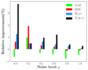
Figure 9: Comparisons of models trained with MSE, MAE, HSIC loss, $I_{\alpha}^{*}(\mathbf{x};e)$ and $H_{\alpha}(e)$ under Gaussian noise $\epsilon\sim\mathcal{N}(0,\rho)$. Each bar denotes the relative performance gain (or loss) over MSE. Only $I_{\alpha}^{*}(\mathbf{x};e)$ and $H_{\alpha}(e)$ perform better than MSE under heavy Gaussian noises.

Understanding the Dynamics of CNNs

We show in the main paper that our measures $T_{\alpha}^{*}$ and $I_{\alpha}^{*}$ reveal two properties behind the training of CNNs: 1) the increase of total amount of dependence amongst all feature maps $C^{1},C^{2},\cdots,C^{N_{t}}$; 2) the movement and stabilization of pairwise dependence occur much earlier in lower layers, compared with that in upper layers. In this section, we show that similar observations have also been made by HSIC (see Figs. 10 and 11). Note that, HSIC only applies for two random variables (here refers to two feature maps). In order to obtain the total amount of dependence, we follow the procedure in (Gretton et al. 2005) and take the average of the sum of all pairwise dependence, i.e., $\frac{1}{N_{t}(N_{t}-1)}\sum_{i=1}^{N}\sum_{j\neq i}\mathrm{HSIC}(C^{i},C^{j})$.

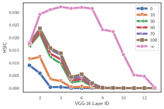
Figure 10: Mean of the sum of all pairwise HSIC scores across training epochs for different convolutional layers.

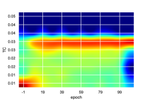
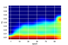
Figure 11: The histogram of HSIC in (a) averaged from the 1st to the 7th CONV layers; and (b) averaged from the 8th to 13th CONV layer. Feature maps reach high dependence with less than 20 epochs of training in lower layers, but need more than 100 epochs in upper layers.

Appendix G The Deep Deterministic Information Bottleneck

We finally present our preliminary results on parameterizing Tishby et al. information bottleneck (IB) principle (Tishby, Pereira, and Bialek 1999) with a neural network. We term our methodology Deep Deterministic Information Bottleneck (DIB), as it avoids variational inference and distribution assumption. We show that deep neural networks trained with DIB outperform the variational objective counterpart and those that are trained with other forms of regularization, in terms of generalization performance.

The IB is an information-theoretic framework for learning. It considers extracting information about a target signal $Y$ through a correlated observable $X$. The extracted information is quantified by a variable $T=T(X)$, which is (a possibly randomized) function of $X$, thus forming the Markov chain $Y\leftrightarrow X\leftrightarrow T$. Suppose we know the joint distribution $p(X,Y)$, the objective is to learn a representation $T$ that maximizes its predictive power to $Y$ subjects to some constraints on the amount of information that it carries about $X$:

$$\mathcal{L}_{IB}=I(Y;T)-\beta I(X;T),$$ (43)

where $I(\cdot;\cdot)$ denotes the mutual information. $\beta$ is a Lagrange multiplier that controls the trade-off between the sufficiency (the performance on the task, as quantified by $I(Y;T)$) and the minimality (the complexity of the representation, as measured by $I(X;T)$). In this sense, the IB principle also provides a natural approximation of minimal sufficient statistic.

The IB objective contains two mutual information terms: $I(X;T)$ and $I(Y;T)$. When parameterizing IB objective with a DNN, $T$ refers to the latent representation of one hidden layer. The maximization of $I(Y;T)$ can be replaced by the minimization of a classic cross-entropy loss (Amjad and Geiger 2019). The same trick has also been used in nonlinear information bottleneck (NIB) (Kolchinsky, Tracey, and Wolpert 2019) and variational information bottleneck (VIB) (Alemi et al. 2017). In this sense, our objective can be interpreted as a cross-entropy loss regularized by a weighted differentiable mutual information term $I(X;T)$. One can simply estimate $I(X;T)$ (in a mini-batch) with our proposed dependence measure (i.e., Eq. (14) or Eq. (16)) in this work.

As a preliminary experiment, we first evaluate the performance of DIB objective on the standard MNIST digit recognition task. We randomly select $10k$ images from the training set as the validation set for hyper-parameter tuning. For a fair comparison, we use the same architecture as has been adopted in (Alemi et al. 2017), namely a MLP with fully connected layers of the form $784-1024-1024-256-10$, and ReLu activation. The bottleneck layer is the one before the softmax layer, i.e., the hidden layer with $256$ units. The Adam optimizer is used with an initial learning rate of 1$e$-4 and exponential decay by a factor of $0.97$ every $2$ epochs. All models are trained with $200$ epochs with mini-batch of size $100$. Table 5 shows the test error of different methods. DIB performs the best.

Table 5: Test error (%) for permutation-invariant MNIST

[t] Model Test (%) Baseline 1.38 Dropout 1.28 Label Smoothing (Pereyra et al. 2017) 1.24 Confidence Penalty (Pereyra et al. 2017) 1.23 VIB (Alemi et al. 2017) 1.17¹ DIB ($\beta$=1$e$-6) 1.13

• Result obtained on our test environment with authors’ code https://github.com/alexalemi/vib˙demo.

In our second experiment, we use VGG16 (Simonyan and Zisserman 2015b) as the baseline network and compare the performance of VGG16 trained by DIB objective and other regularizations. Again, we view the last fully connected layer before the softmax layer as the bottleneck layer. All models are trained with $400$ epochs, a batch-size of $100$, and an initial learning rate $0.1$. The learning rate was reduced by a factor of $10$ for every $100$ epochs. We use SGD optimizer with weight decay 5$e$-4. We explored $\beta$ ranging from 1$e$-4 to $1$, and found that $0.01$ works the best. Test error rates with different methods are shown in Table 6. As can be seen, VGG16 trained with our DIB outperforms other regularizations and also the baseline ResNet50. We also observed, surprisingly, that VIB does not provide performance gain in this example, even though we use the authors’ recommended value of $\beta$ ($0.01$).

Table 6: Test error (%) on CIFAR-10

Model	Test(%)
VGG16	7.36
ResNet18	6.98
ResNet50	6.36
VGG16+Confidence Penalty	5.75
VGG16+Label smoothing	5.78
VGG16+VIB	9.31
VGG16+DIB ($\beta$=1$e$-2)	5.66

References

- Abadi et al. (2016) Abadi, M.; Barham, P.; Chen, J.; Chen, Z.; Davis, A.; Dean, J.; Devin, M.; Ghemawat, S.; Irving, G.; Isard, M.; et al. 2016. Tensorflow: A system for large-scale machine learning. In 12th USENIX symposium on operating systems design and implementation (OSDI 16), 265–283.
- Abdallah and Plumbley (2012) Abdallah, S. A.; and Plumbley, M. D. 2012. A measure of statistical complexity based on predictive information with application to finite spin systems. Physics Letters A 376(4): 275–281.
- Alemi et al. (2017) Alemi, A. A.; Fischer, I.; Dillon, J. V.; and Murphy, K. 2017. Deep variational information bottleneck. In International Conference on Learning Representations.
- Amjad and Geiger (2019) Amjad, R. A.; and Geiger, B. C. 2019. Learning representations for neural network-based classification using the information bottleneck principle. IEEE Transactions on Pattern Analysis and Machine Intelligence 42(9): 2225–2239.
- Austin (2018) Austin, T. 2018. Multi-variate correlation and mixtures of product measures. arXiv preprint arXiv:1809.10272 .
- Bach and Jordan (2002) Bach, F. R.; and Jordan, M. I. 2002. Kernel independent component analysis. Journal of Machine Learning Research 3: 1–48.
- Bay and Schwabacher (2003) Bay, S. D.; and Schwabacher, M. 2003. Mining distance-based outliers in near linear time with randomization and a simple pruning rule. In ACM SIGKDD, 29–38.
- Belghazi et al. (2018) Belghazi, M. I.; Baratin, A.; Rajeshwar, S.; Ozair, S.; Bengio, Y.; Courville, A.; and Hjelm, D. 2018. Mutual information neural estimation. In ICML, 531–540.
- Beyer et al. (1999) Beyer, K.; Goldstein, J.; Ramakrishnan, R.; and Shaft, U. 1999. When is “nearest neighbor” meaningful? In International Conference on Database Theory, 217–235. Springer.
- Bhatia (2006) Bhatia, R. 2006. Infinitely divisible matrices. The American Mathematical Monthly 113(3): 221–235.
- Breunig et al. (2000) Breunig, M. M.; Kriegel, H.-P.; Ng, R. T.; and Sander, J. 2000. LOF: identifying density-based local outliers. In ACM SIGMOD, 93–104.
- Chen et al. (2009) Chen, B.; Hu, J.-C.; Zhu, Y.; and Sun, Z.-Q. 2009. Information theoretic interpretation of error criteria. Acta Automatica Sinica 35(10): 1302–1309.
- Chen et al. (2016a) Chen, B.; Xing, L.; Xu, B.; Zhao, H.; and Principe, J. C. 2016a. Insights into the robustness of minimum error entropy estimation. IEEE Transactions on Neural Networks and Learning Systems 29(3): 731–737.
- Chen et al. (2010) Chen, B.; Zhu, Y.; Hu, J.; and Zhang, M. 2010. A new interpretation on the MMSE as a robust MEE criterion. Signal Processing 90(12): 3313–3316.
- Chen et al. (2016b) Chen, L.; Qu, H.; Zhao, J.; Chen, B.; and Principe, J. C. 2016b. Efficient and robust deep learning with correntropy-induced loss function. Neural Computing and Applications 27(4): 1019–1031.
- Chung et al. (1986) Chung, F. R.; Graham, R. L.; Frankl, P.; and Shearer, J. B. 1986. Some intersection theorems for ordered sets and graphs. Journal of Combinatorial Theory, Series A 43(1): 23–37.
- Cover (1999) Cover, T. M. 1999. Elements of information theory. John Wiley & Sons.
- Demšar (2006) Demšar, J. 2006. Statistical comparisons of classifiers over multiple data sets. Journal of Machine learning research 7(Jan): 1–30.
- Erdogmus and Principe (2002) Erdogmus, D.; and Principe, J. C. 2002. An error-entropy minimization algorithm for supervised training of nonlinear adaptive systems. IEEE Transactions on Signal Processing 50(7): 1780–1786.
- Fanaee-T and Gama (2014) Fanaee-T, H.; and Gama, J. 2014. Event labeling combining ensemble detectors and background knowledge. Progress in Artificial Intelligence 2(2-3): 113–127.
- Feng, Loparo, and Fang (1997) Feng, X.; Loparo, K. A.; and Fang, Y. 1997. Optimal state estimation for stochastic systems: An information theoretic approach. IEEE Transactions on Automatic Control 42(6): 771–785.
- Fernandes and Gloor (2010) Fernandes, A. D.; and Gloor, G. B. 2010. Mutual information is critically dependent on prior assumptions: would the correct estimate of mutual information please identify itself? Bioinformatics 26(9): 1135–1139.
- Greenfeld and Shalit (2020) Greenfeld, D.; and Shalit, U. 2020. Robust learning with the Hilbert-Schmidt independence criterion. In ICML, 3759–3768.
- Gretton et al. (2012) Gretton, A.; Borgwardt, K. M.; Rasch, M. J.; Schölkopf, B.; and Smola, A. 2012. A kernel two-sample test. Journal of Machine Learning Research 13(Mar): 723–773.
- Gretton et al. (2005) Gretton, A.; Bousquet, O.; Smola, A.; and Schölkopf, B. 2005. Measuring statistical dependence with Hilbert-Schmidt norms. In International Conference on Algorithmic Learning Theory, 63–77. Springer.
- Gretton et al. (2008) Gretton, A.; Fukumizu, K.; Teo, C. H.; Song, L.; Schölkopf, B.; and Smola, A. J. 2008. A kernel statistical test of independence. In NeurIPS, 585–592.
- Hinton et al. (2012) Hinton, G. E.; Srivastava, N.; Krizhevsky, A.; Sutskever, I.; and Salakhutdinov, R. R. 2012. Improving neural networks by preventing co-adaptation of feature detectors. arXiv preprint arXiv:1207.0580 .
- Hu et al. (2013) Hu, T.; Fan, J.; Wu, Q.; and Zhou, D.-X. 2013. Learning theory approach to minimum error entropy criterion. Journal of Machine Learning Research 14(Feb): 377–397.
- Joe (1989) Joe, H. 1989. Relative entropy measures of multivariate dependence. Journal of the American Statistical Association 84(405): 157–164.
- Josse and Holmes (2016) Josse, J.; and Holmes, S. 2016. Measuring multivariate association and beyond. Statistics Surveys 10: 132.
- Kalata and Priemer (1979) Kalata, P.; and Priemer, R. 1979. Linear prediction, filtering, and smoothing: An information-theoretic approach. Information Sciences 17(1): 1–14.
- Keller, Muller, and Bohm (2012) Keller, F.; Muller, E.; and Bohm, K. 2012. HiCS: High contrast subspaces for density-based outlier ranking. In ICDE, 1037–1048. IEEE.
- Kingma and Ba (2014) Kingma, D. P.; and Ba, J. 2014. Adam: A method for stochastic optimization. arXiv preprint arXiv:1412.6980 .
- Kingma and Welling (2014) Kingma, D. P.; and Welling, M. 2014. Auto-Encoding Variational Bayes. In ICLR.
- Kolchinsky, Tracey, and Wolpert (2019) Kolchinsky, A.; Tracey, B. D.; and Wolpert, D. H. 2019. Nonlinear information bottleneck. Entropy 21(12): 1181.
- Kraskov, Stögbauer, and Grassberger (2004) Kraskov, A.; Stögbauer, H.; and Grassberger, P. 2004. Estimating mutual information. Physical Review E 69(6): 066138.
- Kriegel, Schubert, and Zimek (2008) Kriegel, H.-P.; Schubert, M.; and Zimek, A. 2008. Angle-based outlier detection in high-dimensional data. In ACM SIGKDD, 444–452.
- Krizhevsky (2009) Krizhevsky, A. 2009. Learning multiple layers of features from tiny images. Technical report, University of Toronto.
- Lazarevic and Kumar (2005) Lazarevic, A.; and Kumar, V. 2005. Feature bagging for outlier detection. In ACM SIGKDD, 157–166.
- Lopez-Paz, Hennig, and Schölkopf (2013) Lopez-Paz, D.; Hennig, P.; and Schölkopf, B. 2013. The randomized dependence coefficient. In NeurIPS, 1–9.
- MacKay (2003) MacKay, D. J. 2003. Information theory, inference and learning algorithms. Cambridge university press.
- Madiman and Tetali (2010) Madiman, M.; and Tetali, P. 2010. Information inequalities for joint distributions, with interpretations and applications. IEEE Transactions on Information Theory 56(6): 2699–2713.
- Magnus (1985) Magnus, J. R. 1985. On differentiating eigenvalues and eigenvectors. Econometric Theory 179–191.
- Marbach et al. (2012) Marbach, D.; Costello, J. C.; Küffner, R.; Vega, N. M.; Prill, R. J.; Camacho, D. M.; Allison, K. R.; Kellis, M.; Collins, J. J.; and Stolovitzky, G. 2012. Wisdom of crowds for robust gene network inference. Nature Methods 9(8): 796–804.
- Müller et al. (2009) Müller, E.; Assent, I.; Günnemann, S.; Krieger, R.; and Seidl, T. 2009. Relevant subspace clustering: Mining the most interesting non-redundant concepts in high dimensional data. In ICDM, 377–386. IEEE.
- Nguyen et al. (2014) Nguyen, H. V.; Müller, E.; Vreeken, J.; Efros, P.; and Böhm, K. 2014. Multivariate maximal correlation analysis. In ICML, 775–783.
- Nguyen et al. (2013) Nguyen, H. V.; Müller, E.; Vreeken, J.; Keller, F.; and Böhm, K. 2013. CMI: An information-theoretic contrast measure for enhancing subspace cluster and outlier detection. In SIAM International Conference on Data Mining, 198–206. SIAM.
- Paszke et al. (2019) Paszke, A.; Gross, S.; Massa, F.; Lerer, A.; Bradbury, J.; Chanan, G.; Killeen, T.; Lin, Z.; Gimelshein, N.; Antiga, L.; et al. 2019. Pytorch: An imperative style, high-performance deep learning library. In NeurIPS, 8026–8037.
- Pereyra et al. (2017) Pereyra, G.; Tucker, G.; Chorowski, J.; Kaiser, Ł.; and Hinton, G. 2017. Regularizing neural networks by penalizing confident output distributions. In International Conference on Learning Representations (workshop).
- Poczos, Ghahramani, and Schneider (2012) Poczos, B.; Ghahramani, Z.; and Schneider, J. 2012. Copula-based kernel dependency measures. In ICML.
- Principe et al. (2000) Principe, J. C.; Xu, D.; Zhao, Q.; and Fisher, J. W. 2000. Learning from examples with information theoretic criteria. Journal of VLSI Signal Processing Systems for Signal, Image and Video Technology 26(1-2): 61–77.
- Quionero-Candela et al. (2009) Quionero-Candela, J.; Sugiyama, M.; Schwaighofer, A.; and Lawrence, N. D. 2009. Dataset shift in machine learning. The MIT Press.
- Raghu et al. (2017) Raghu, M.; Gilmer, J.; Yosinski, J.; and Sohl-Dickstein, J. 2017. Svcca: Singular vector canonical correlation analysis for deep learning dynamics and interpretability. In NeurIPS, 6076–6085.
- Rao et al. (2004) Rao, M.; Chen, Y.; Vemuri, B. C.; and Wang, F. 2004. Cumulative residual entropy: a new measure of information. IEEE Transactions on Information Theory 50(6): 1220–1228.
- Rayana (2016) Rayana, S. 2016. ODDS Library. http://odds.cs.stonybrook.edu. Stony Brook University, Department of Computer Sciences.
- Rényi (1959) Rényi, A. 1959. On measures of dependence. Acta Mathematica Academiae Scientiarum Hungarica 10(3-4): 441–451.
- Reshef et al. (2011) Reshef, D. N.; Reshef, Y. A.; Finucane, H. K.; Grossman, S. R.; McVean, G.; Turnbaugh, P. J.; Lander, E. S.; Mitzenmacher, M.; and Sabeti, P. C. 2011. Detecting novel associations in large data sets. Science 334(6062): 1518–1524.
- Romano et al. (2016) Romano, S.; Chelly, O.; Nguyen, V.; Bailey, J.; and Houle, M. E. 2016. Measuring dependency via intrinsic dimensionality. In ICPR, 1207–1212. IEEE.