No Scalar-Haired Cauchy Horizon Theorem in Einstein-Maxwell-Horndeski Theories

Abstract

Recently, a no inner (Cauchy) horizon theorem for static black holes with non-trivial scalar hairs has been proved in Einstein-Maxwell-scalar theories. In this paper, we study an extension of the theorem to the static black holes in Einstein-Maxwell-Horndeski theories. We study the black hole interior geometry for some exact solutions and find that the spacetime has a (space-like) curvature singularity where the black hole mass gets an extremum and the Hawking temperature vanishes. We discuss further extensions of the theorem, including general Horndeski theories from disformal transformations.

Exploring the interior structure of black holes has been a fundamental topic in general relativity (GR) but much are not well understood yet. For example, whether the interior spacetime is singular or not for the real black holes in nature as observed in various ways Abbo:2016 ; Akiy:2019 . The other question, which is relevant to this paper is whether the (classical) predictability in GR is lost due to the inner (Cauchy) horizons as in the exact solutions, like Reissner-Nordstrom, Kerr black holes. Regarding the latter question, recent development suggests that Cauchy horizons for some kind of charged black holes are unstable in the presence of scalar hairs Hart:2012 ; Cai:2020 . In particular, in Cai:2020 it is proved that there exists no inner Cauchy horizons for both planar and spherical static black holes with non-trivial scalar hairs in Einstein-Maxwell-scalar theories. From the simplicity and quite generic results, which do not depend on the details of the scalar potentials as well as the spacetime structure at the short distance, it’s applicability would be quite far-reaching. In this respect, it would be important to classify all possible extensions of the theorem.

In this paper, as the first step towards that goal, we consider an extension of the theorem to the black holes in Einstein-Maxwell-Horndeski (EMH) theories, with a quartic Horndeski term Hord:1974 . To this ends, we consider the $D$-dimensional EMH action, with the $U(1)$ gauge filed $A_{\mu}$ and charged scalar field $\varphi$,

$$I = \int d^{D}x\sqrt{-g}\left[\frac{1}{\kappa}R+{\cal L}_{m}\right],$$ (1)

$${\cal L}_{m} = -\frac{Z(|\varphi|^{2})}{4\kappa}F_{\mu\nu}F^{\mu\nu}-\left({\alpha}g^{\mu\nu}-\gamma G^{\mu\nu}\right)(D_{\mu}\varphi)^{*}(D_{\nu}\varphi)-V(|\varphi|^{2}),{}$$

where $F_{\mu\nu}\equiv\nabla_{\mu}A_{\nu}-\nabla_{\nu}A_{\mu}$ and $D_{\mu}\equiv\nabla_{\mu}-iqA_{\mu}$ with a scalar field charge $q$ and $\kappa\equiv 16\pi G$. Here, we have introduced $Z$ and $V$ as arbitrary functions of $|\varphi|^{2}$ in which the constant shift symmetry of the Horndeski terms, with a non-minimal (derivative) coupling ${\gamma}$ of the scalar field to the Einstein tensor $G^{\mu\nu}\equiv R^{\mu\nu}-(1/2)g^{\mu\nu}R$ as well as the usual minimal coupling ${\alpha}$, may be broken generally. Note that this generalizes the recent set-up in Hart:2012 ; Cai:2020 into higher-derivative theories via the Einstein coupling.

Let us then consider the general static ansatz,

$$ds^{2} = -N^{2}(r)dt^{2}+\frac{1}{f(r)}dr^{2}+r^{2}d\Omega^{2}_{D-2,k},$$ (2)

$$\varphi = \varphi(r),~{}A=A_{t}(r)dt,{}$$

where $d\Omega^{2}_{D-2,k}$ is the metric of $(D-2)$-dimensional unit sphere with the spatial curvature which is normalized as $k=1,0,-1$ for the spherical, planar, hyperbolic topologies. The equations of motion [Here, we consider $D=4$ case for simplicity. But its higher-dimensional generalization is straightforward (for the details, see Appendix A) Cai:2020 ; Feng:2015 and we will discuss about this later] are given by (the prime $(^{\prime})$ and the dot $(\dot{~{}})$ denote the derivatives with respect to $r$ and $|\varphi|^{2}$, respectively),

$$E_{A} \equiv \frac{1}{{\kappa}}\left(Z(|\varphi|^{2})\frac{\sqrt{f}}{N}~{}r^{2}A_{t}^{\prime}\right)^{\prime}-\frac{2q^{2}|\varphi|^{2}A_{t}}{f}\left(\frac{\sqrt{f}}{N}\right)\left[{\alpha}r^{2}+{\gamma}(k-f)-{\gamma}rf^{\prime}\right]=0,$$ (3)

$$E_{\varphi} \equiv \left(\frac{N}{\sqrt{f}}f\left[{\alpha}r^{2}+{\gamma}(k-f)-{\gamma}rf\left(\frac{{N^{2}}^{\prime}}{N^{2}}\right)\right]\varphi^{\prime}\right)^{\prime}{}$$ (4)

$$+\left(\frac{N}{\sqrt{f}}\right)\frac{q^{2}A_{t}^{2}\varphi}{N^{2}}\left[{\alpha}r^{2}+{\gamma}(k-f)-{\gamma}rf^{\prime}\right]+r^{2}\left[\frac{1}{2{\kappa}}\frac{\sqrt{f}}{N}\dot{Z}{A_{t}^{\prime}}^{2}-\frac{N}{\sqrt{f}}~{}\dot{V}\right]\varphi=0,$$

$$E_{N} \equiv \frac{2}{{\kappa}}\left(f-k+{rf^{\prime}}\right)+r^{2}V(|\varphi|^{2})+f\left[{\alpha}r^{2}+{\gamma}(k+f)+3{\gamma}rf^{\prime}\right]|\varphi^{\prime}|^{2}{}$$ (5)

$$+2{\gamma}rf^{2}\left(|\varphi^{\prime}|^{2}\right)^{\prime}+\frac{1}{2N^{2}}\left(\frac{1}{{\kappa}}{Z}fr^{2}{A_{t}^{\prime}}^{2}+2q^{2}|\varphi|^{2}A_{t}^{2}\left[{\alpha}r^{2}+{\gamma}(k-f)-{\gamma}rf^{\prime}\right]\right)=0,$$

$$E_{f} \equiv \frac{2}{{\kappa}}\left[f-k+{rf}\left(\frac{{N^{2}}^{\prime}}{N^{2}}\right)\right]+r^{2}V(|\varphi|^{2})-f\left[{\alpha}r^{2}+{\gamma}(k-3f)-3{\gamma}rf\left(\frac{{N^{2}}^{\prime}}{N^{2}}\right)\right]|\varphi^{\prime}|^{2}{}$$ (6)

$$+\frac{1}{2N^{2}}\left(\frac{1}{{\kappa}}{Z}fr^{2}{A_{t}^{\prime}}^{2}-2q^{2}|\varphi|^{2}A_{t}^{2}\left[{\alpha}r^{2}+{\gamma}(k-f)\right]\right){}$$

$$+\frac{{\gamma}q^{2}}{N^{2}}\left(|\varphi|^{2}\left[-rfA_{t}^{2}\left(\frac{{N^{2}}^{\prime}}{N^{2}}\right)+2rf(A_{t}^{2})^{\prime}\right]+2rfA_{t}^{2}(|\varphi|^{2})^{\prime}\right)=0,$$

where the first two equations (3), (4) are the equations for the gauge field and scalar field respectively and the last two (5), (6) are for the metric. In particular, (3) and (5) correspond to the Gauss’s law constraint and Hamiltonian constraint equations in canonical formulation, respectively. Even though it is difficult to solve the coupled non-linear PDE generally, several exact solutions are known for some specific choices of couplings and potentials. We will study the black hole interior geometry for those exact solutions in details. But before this, we first prove the “no scalar-haired Cauchy horizon theorem” quite generally, without knowing the details of the interior geometry, which extends the argument of Cai:2020 for Einstein-Maxwell-scalar theories into the EMH theory with a non-vanishing Einstein coupling ${\gamma}$.

No Scalar-Haired Cauchy Horizon Theorem: The proof depends on whether the scalar field is charged or not. Let us first consider the charged scalar field case . Then, suppose that there were a finite-temperature (i.e., non-extremal) black hole with the outer and inner (Cauchy) horizons at $r_{+}$ and $r_{-}(<r_{+})$, respectively (Fig. 1), i.e.

$$N^{2}(r_{+})=f(r_{+})=0,~{}{N^{2}}^{\prime}(r_{+}),f^{\prime}(r_{+})>0,$$ (7)

$$N^{2}(r_{-})=f(r_{-})=0,~{}{N^{2}}^{\prime}(r_{-}),f^{\prime}(r_{-})\leq 0.$$ (8)

Now, in order to have a “non-trivial”, i.e., finite charged scalar field $\varphi$ at the two horizons, the equations of motion (3 - 6) imply the conditions Cai:2020 (for a more rigorous derivation, see Appendix B),

$$A_{t}(r_{+})=A_{t}(r_{-})=0$$ (9)

from the regularity at the horizons. This regularity condition is one of the key ingredients in the proof.

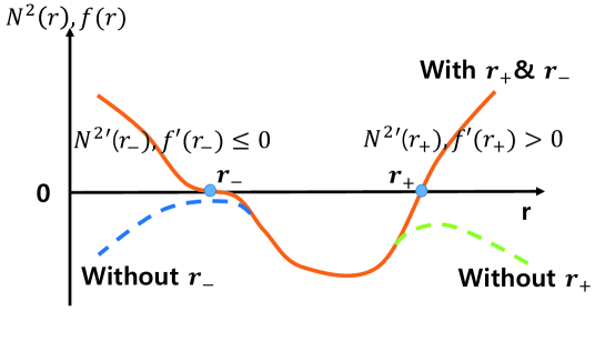
Figure 1: Typical plots of $N^{2}(r)$ and $f(r)$ for a finite-temperature, charged black hole with the inner (Cauchy) horizon $r_{-}$ and outer (event) horizon $r_{+}$. Due to a non-zero Hawking temperature, we have $N^{2}=f=0,~{}{N^{2}}^{\prime},f^{\prime}>0$ at the outer horizon $r_{+}$, whereas $N^{2}=f=0,~{}{N^{2}}^{\prime},f^{\prime}\leq 0$ at the inner horizon generally, if existed (orange, solid line). In the absence of an inner horizon, ${N^{2}}^{\prime},f^{\prime}$ can have arbitrary values but there is no inner point of $N^{2}=f=0$ (blue, dashed line). On the other hand, in the absence of outer horizon but now with an inner horizon, the situation is similar for an observer sitting inside the inner horizon which becomes now an event horizon (green, dashed line).

Another key ingredient is the existence of radially conserved charge,

$${\cal Q} = (D-2)r^{D-2}\left[N\sqrt{f}\left(\frac{1}{{\kappa}}+\frac{{\gamma}}{2}f|\varphi^{\prime}|^{2}\right)\left(\frac{{N^{2}}^{\prime}}{N^{2}}-\frac{2}{r}\right)-\frac{1}{2{\kappa}}\frac{\sqrt{f}}{N}Z{A_{t}^{2}}^{\prime}\right.{}$$ (10)

$$+\left.\frac{\sqrt{f}}{N}{\gamma}q^{2}A_{t}^{2}|\varphi|^{2}\left(\frac{2A_{t}^{\prime}}{A_{t}}-\frac{{N^{2}}^{\prime}}{2N^{2}}-\frac{1}{r}\right)+\frac{\sqrt{f}}{N}{\gamma}q^{2}A_{t}^{2}{|\varphi|^{2}}^{\prime}\right]{}$$

$$+k(D-2)(D-3)\int^{r}dx~{}x^{D-4}\left[\frac{{\gamma}q^{2}A_{t}^{2}|\varphi|^{2}}{\sqrt{N^{2}f}}+\frac{N}{\sqrt{f}}\left(\frac{2}{{\kappa}}-{{\gamma}}f|\varphi^{\prime}|^{2}\right)\right],$$

where we have recovered the dimensional dependencies. From the equations of motion (3) - (6), one can prove that ${\cal Q}$ is radially conserved, i.e., r-independent, due to a (remarkable) relation ,

$${\cal Q}^{\prime} = 2\frac{\sqrt{f}}{N}\left[r\left(\frac{N^{2}}{f}{{\cal E}_{f}}^{\prime}+\frac{1}{2}\frac{{N^{2}}^{\prime}}{f}{\cal E}_{f}\right)+\left((D-2)\frac{N^{2}}{f}+\frac{r}{2}\frac{{N^{2}}^{\prime}}{f}\right){\cal E}_{N}\right.{}$$ (11)

$$\left.+\frac{r}{2}N^{2}\varphi^{\prime}~{}{\cal E}_{\varphi}+\frac{1}{2}\left((D-2)A_{t}+rA_{t}^{\prime}\right){\cal E}_{A}\right]=0,$$

where ${\cal E}_{\psi}$’s represent the equations of motion for the fields $\psi=(N,f,\varphi,A_{t})$ which can be obtained directly from the action and related to $E_{\psi}$’s in (3) -(6) as ${\cal E}_{N}=-E_{N}r^{D-4}/2,~{}{\cal E}_{f}=E_{f}r^{D-4}/2,~{}{\cal E}_{\varphi}=2E_{\varphi}/N\sqrt{f},~{}{\cal E}_{A}=-E_{A}N/\sqrt{f}$.

For the planar topology, $k=0$, the first line of (10) is a Noether charge associated with a particular scaling symmetry for a neutral scalar field with $q=0$ Feng:2015 ; Gubs:2009 . For other topologies $k\neq 0$, the local parts in the first and second lines are not conserved but the non-local, integrated terms are needed in order that the non-conserved terms are canceled Cai:2020 .

Now, due to the $r$-independence, the charge satisfies ${\cal Q}_{r_{+}}={\cal Q}_{r_{-}}$ at the two horizons, in particular, where the boundary conditions (7), (8), and (9) hold, we have the relation

$$\frac{(D-2)}{{\kappa}}\left[r_{+}^{D-2}\frac{\sqrt{f}}{N}\left.{N^{2}}^{\prime}\right|_{r_{+}}-r_{-}^{D-2}\frac{\sqrt{f}}{N}\left.{N^{2}}^{\prime}\right|_{r_{-}}\right]{}$$ (12)

$$= k(D-2)(D-3)\int^{r_{+}}_{r_{-}}dx~{}x^{D-4}\left[-\frac{{\gamma}q^{2}A_{t}^{2}|\varphi|^{2}}{\sqrt{N^{2}f}}+\frac{N}{\sqrt{f}}\left(-\frac{2}{{\kappa}}+{{\gamma}}f|\varphi^{\prime}|^{2}\right)\right].$$

From the assumed inner horizon $r_{-}$, i.e., ${N^{2}}^{\prime}\sqrt{f}/N|_{r_{-}}\leq 0$, as well as the outer horizon $r_{+}$ with a non-vanishing Hawking temperature or surface gravity $\sim{N^{2}}^{\prime}\sqrt{f}/N|_{r_{+}}>0$, the left hand side of (12) is positive. On the other hand, the integrand on the right hand side is negative for the “positive” Horndeski coupling constant ${\gamma}>0$ due to the space-time structure between $r_{+}$ and $r_{-}$, where $N^{2},f<0$, so that (12) is inconsistent unless the hyperbolic topology $k=-1$ is considered. In other words, no smooth inner (Cauchy) horizon with the outer horizon can be formed for $k=0$ or $k=1$ and this generalizes the theorem of Hart:2012 ; Cai:2020 to a class of the EMH theories (1) with the positive Einstein coupling ${\gamma}>0$. However, for a negative Einstein coupling ${\gamma}<0$, one can not get a strong constraint on the inner horizon, due to lack of a definite sign of the integrand on (12), except the case $k=0$ in which the above theorem still works. Here, it interesting to note that the theorem may also imply the no outer horizon with an inner horizon as described in Fig.1 (green, dashed line). This completes the proof of the theorem for the charged scalar field with $q\neq 0$ and note that the proof is quite generic without assuming any specific form of the scalar potential.

On the other hand, for the $k=-1$ (${\gamma}>0$) case, the relation (12) can be consistent with the inner horizon but it can be still consistent even without the inner horizon, i.e., ${N^{2}}^{\prime}\sqrt{f}/N|_{r_{-}}>0$ unless its contribution dominates that of the outer horizon in the left hand side so that (12) is still satisfied. In this sense, the theorem does not give any strong constraint about the inner horizon formation for the $k=-1$ case, except the possibility of its formation. Moreover, for the neutral scalar field ($q=0$), the vanishing gauge field (9) can not be justified anymore and there is no constraint on gauge field from the regularity at the horizons so that the novel relation (12) can not be used for the proof and we need a separate consideration as described below. However, we note that the same theorem also applies to neutral black holes, i.e., in the absence of $U(1)$ gauge field $A_{\mu}$, since the essential parts of (12) do not depend on it.

For the proof of neutral scalar field, following Hart:2012 , we multiply $\varphi^{*}$ to (4) and obtain

$$0 = \int^{r_{+}}_{r_{-}}\left(\frac{N}{\sqrt{f}}~{}f\left[{\alpha}r^{2}+{\gamma}(k-f)-{\gamma}rf\left(\frac{{N^{2}}^{\prime}}{N^{2}}\right)\right]\varphi^{*}\varphi^{\prime}\right)^{\prime}{}$$ (13)

$$= \int^{r_{+}}_{r_{-}}\frac{N}{\sqrt{f}}\left\{f\left[{\alpha}r^{2}+{\gamma}(k-f)-{\gamma}rf\left(\frac{{N^{2}}^{\prime}}{N^{2}}\right)\right]|\varphi^{\prime}|^{2}-r^{2}\left[\frac{1}{{\kappa}}\frac{f}{N^{2}}\dot{Z}{A_{t}^{\prime}}^{2}-\dot{V}\right]|\varphi|^{2}\right.{}$$

$$~{}~{}~{}~{}~{}~{}~{}~{}~{}~{}\left.-\frac{q^{2}A_{t}^{2}|\varphi|^{2}}{N^{2}}\left[{\alpha}r^{2}+{\gamma}(k-f)-{\gamma}rf^{\prime}\right]\right\}.$$

For the neutral scalar field with $q=0$, where the last term in the third line is absent, the integrand in the second line is non-positive if the quantities in $[~{}~{}]$ for first and second terms in the second line are “positive”. In this case, the second line is consistent with the first line only for the vanishing scalar field $\varphi=0$ in the range of $(r_{-},r_{+})$, which means the impossibility of inner (Cauchy) horizon with a non-trivial scalar field (i.e., hair) and an outer (event) horizon, or similarly the impossibility of an outer horizon with a non-trivial scalar field and an inner horizon, as in the charged case. For the Einstein-Maxwell-scalar theories with ${\alpha}>0,{\gamma}=0$ as in Hart:2012 ; Cai:2020 , the required condition for the theorem is $\dot{Z}{A_{t}^{\prime}}^{2}{f}/{N^{2}}{\kappa}-\dot{V}>0$. With the Horndeski coupling ${\gamma}$, we may need a further condition, like ${\alpha}r^{2}+{\gamma}(k-f)-{\gamma}rf{{N^{2}}^{\prime}}/{N^{2}}>0$. This produces the constraint on the range, $r<{{(N^{2}/f)}[{\alpha}r^{2}+{\gamma}(k-f)]}/{{{\gamma}}{N^{2}}^{\prime}}$, near $r_{+}$ (or equivalently near $r_{-}$) with ${{\gamma}}{N^{2}}^{\prime}>0$ for the validity of the theorem, which could imply the non-vanishing scalar field in the black hole interior near $r_{+}$ (or exterior near $r_{-}$). On the other hand, in the presence of a charge $q$, the last term gets a positive contribution even if the above conditions are satisfied so that one can not generally rule out the inner (or outer) horizon formations, as noted in Cai:2020 , unless we need more conditions on the metric and matter fields or electric charge.

An Example of Interior Geometry with Inner Horizon

Now, in order to study explicitly the interior geometry of a charged black hole with a non-trivial scalar field, we consider an exact solution for ${\alpha}=0$ (no minimal scalar coupling), $q=0$ (neutral scalar field), $Z=1$ (minimal gauge coupling), $V=2{\Lambda}/\kappa$ (cosmological constant term, no self-scalar-coupling) in $D=4$, for simplicity (for $k=1$, see Anab:2014 ; Cist:2014 ; Feng:2015 and also Rina:2012 ; Babi:2013 ) but ${\gamma}\neq 0$ (non-vanishing Einstein tensor-scalar coupling),

$$N^{2} = k\left(k^{2}+\frac{{\Lambda}\bar{q}^{2}}{8}\right)-\frac{M}{r}+\frac{k^{2}}{4}\frac{\bar{q}^{2}}{r^{2}}-\frac{k}{192}\frac{\bar{q}^{4}}{r^{4}}-\frac{k^{2}{\Lambda}}{3}r^{2}+\frac{k{\Lambda}^{2}}{20}r^{4},$$ (14)

$$\frac{f}{N^{2}} = \frac{64r^{4}}{(4{\Lambda}r^{4}-8kr^{2}+\bar{q}^{2})^{2}},$$ (15)

$$A_{t} = A_{t}^{(0)}-\frac{k\bar{q}}{r}+\frac{\bar{q}^{3}}{24r^{3}}-\frac{\bar{q}{\Lambda}}{2}r,$$ (16)

$$\varphi^{\prime} = \sqrt{\frac{4{\Lambda}r^{2}+{\bar{q}^{2}}/{r^{2}}}{-4{\gamma}k{\kappa}f}},$$ (17)

where $M$ and $\bar{q}$ represent the two integration constants, associated with the black hole mass and charge, respectively. Here, we note that the solution can be defined only when ${\gamma}\neq 0$ is considered though not manifest in the metric and gauge field solutions. But interestingly, the solution for $k=\pm 1$, pure Einstein-Maxwell theories with a scalar field, i.e., ${\alpha}={\gamma}=0$, can be also read with a certain truncation of higher-order terms,

$$N^{2} = f=k-\frac{M}{r}+\frac{1}{4}\frac{\bar{q}^{2}}{r^{2}}-\frac{{\Lambda}}{3}r^{2},$$ (18)

$$A_{t} = A_{t}^{(0)}-\frac{k\bar{q}}{r},$$ (19)

which seems to imply a smooth limit of ${\gamma}\rightarrow 0$.

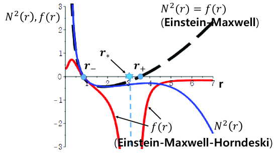
Figure 2: Plots of $N^{2}(r)$ (blue line) and $f(r)$ (red line) for a charged black hole solution (14), (15) with $k=-1,M<0$ in ant-de Sitter space ${\Lambda}<0$. Due to a Horndeski coupling ${\gamma}\neq 0$, the metric function $f$ is divergent at $r_{*}\approx 3.18$ where a (space-like) curvature singularity occurs, in addition to the usual singularity at $r=0$. Moreover, even with the inner horizon $r_{-}$, no outer horizon $r_{+}$ is formed (red, blue solid lines), in contrast with two horizons in the pure Einstein-Maxwell theories (dashed line). Here, we have considered ${\Lambda}=-0.2,q=1,M=-0.5$.

The metric has a surface-like curvature singularity (we omit the explicit expressions of curvatures due to their messy expressions) at

$$r_{*}=\sqrt{\frac{-k\mp\sqrt{k^{2}-{\Lambda}\bar{q}^{2}/4}}{-{\Lambda}}}$$ (20)

in which $f/N^{2}$ in (15) diverges, as well as the usual point-like singularity at $r=0$ (see Fig. 2, for the case $k=-1,M<0$). When the black hole horizon $r_{H}$ reaches to the singular radius $r_{*}$, i.e. $r_{H}=r_{*}$, the black hole mass parameter $M$,

$$M=k\left(k^{2}+\frac{{\Lambda}\bar{q}^{2}}{8}\right)r_{H}+\frac{k^{2}}{4}\frac{\bar{q}^{2}}{r_{H}}-\frac{k}{192}\frac{\bar{q}^{4}}{r_{H}^{3}}-\frac{k^{2}{\Lambda}}{3}r_{H}^{3}+\frac{k{\Lambda}^{2}}{20}r_{H}^{5}$$ (21)

becomes an extremum value,

$$M_{*}=\frac{[k({\Lambda}^{2}\bar{q}^{4}-12k^{2}{\Lambda}\bar{q}^{2}-32k^{4})\mp 16(2k^{2}+{\Lambda}\bar{q}^{2})\sqrt{k^{2}-{\Lambda}\bar{q}/4}]}{30\sqrt{{\Lambda}}(k\pm\sqrt{k^{2}-{\Lambda}\bar{q}^{2}/4})^{3/2}}.$$ (22)

Moreover, at the extreme horizon radius $r_{H}=r_{*}$, the Hawking temperature ,

$$T_{H} = \left.\frac{\hbar}{4\pi}\left(\frac{N}{\sqrt{f}}\right){N^{2}}^{\prime}\right|_{r_{H}}{}$$ (23)

$$= \frac{\hbar k}{32\pi r_{H}^{3}}\left(8k^{2}r_{H}^{2}-k\bar{q}^{2}-4k{\Lambda}r_{H}^{4}\right)$$

becomes zero.

For the hyperbolic case with $k=-1$ and ${\Lambda},M<0$, there is only a “cosmological” horizon $r_{-}$, which used to be the inner (Cauchy) horizon in the purely Einstein-Maxwell theories without a (neutral) scalar field (dashed line in Fig. 2). In this case, the outer horizon is not formed due to Horndeski coupling ${\gamma}$ of scalar field , which behaves as (with a vanishing integration constant)

$$\varphi =2\left.\sqrt{\frac{rg(r)}{2{\gamma}{\kappa}}}\right|_{r_{-}}~{}\sqrt{r_{-}-r}+{\cal O}(r_{-}-r)^{3/2},$$ (24)

$$g(r) \equiv 4{\Lambda}r^{2}+{\bar{q}^{2}}/r^{2},$$ (25)

near the inner horizon $r_{-}$, implying the vanishing and non-analytic scalar field at the inner horizon when $g(r_{-})/{\gamma}>0$. In the exterior region of the (inner) horizon, $r>r_{-}$, where $r$ is a time coordinate, the scalar field may also exist and behaves as, though non-analytic again, near the surface-like singularity $r_{*}$,

$$\varphi=-\frac{4}{3}\left.\sqrt{\frac{4k^{2}-k\bar{q}^{2}/r^{2}}{2{\gamma}k{\kappa}N^{2}}}~{}\right|_{r_{*}}(r_{*}-r)^{3/2}+{\cal O}(r_{*}-r)^{5/2}$$ (26)

when $g(r)/{\gamma}<0$, i.e., $r_{-}<\tilde{r}<r$ with $g(\tilde{r})=0$ and $\varphi^{\prime}(r_{*})=0$. On the other hand, the gauge field is regular and analytic at the (inner) horizon and has a vanishing electric field, $A_{t}^{\prime}=\frac{\bar{q}}{r^{2}}\frac{N}{\sqrt{f}}$ at $r_{*}$.

Concluding Remarks

As a summary, we have an extension of the “no scalar-haired inner (Cauchy) horizon theorem” to the black holes in a class of the EMH theories with a Einstein coupling ${\gamma}$, which crucially depends on the sign of ${\gamma}$: No charged scalar-haired Cauchy horizon in $k=0,1$ (planar, spherical) black holes for ${\gamma}>0$, whereas only in $k=0$ black holes for ${\gamma}<0$. Here, it is important to note that the proof is quite generic without assuming any specific form of the scalar potential nor the spacetime structure at the short distance. On the other hand, for the neutral scalar field, we need some kinematic conditions for the corresponding theorem, which depends on the details of the system. As an explicit example of the black hole interior geometry with inner horizon, we studied some exact solutions with an inner horizon but no outer horizon due to non-trivial scalar field (hairs). Several further remarks about remaining challenging problems are in order.

1. We have considered a special case of Horndeski terms, with $G_{2}$ and $G_{4}$ in the usual terminology. By considering disformal transformations, $\tilde{g}_{\mu\nu}={A(\varphi)}g_{\mu\nu}+{B(\varphi)}\nabla_{\mu}\varphi\nabla_{\nu}\varphi$, with $X\equiv-g^{\mu\nu}\nabla_{\mu}\nabla_{\nu}\varphi$ one can get the general form of the Horndeski action but with the special coefficients depending on $A$ and $B$ Bett:2013 . Hence, for the obtained Horndeski actions, one can also argue the same no-Cauchy-horizon theorem. It would be interesting to see whether we have the same result for the fully general Horndeski actions or not.

2. The theorem implies that the instability of Cauchy horizon under non-trivial scalar field (linear or non-linear) perturbations. However, the (dynamical) stability of the non-trivial hairy geometry is not be guaranteed generally and its explicit check would be an important complementary for the theorem.

3. In this paper, we have considered the Cauchy horizon for a “spherically symmetric”, charged black hole. It would be a challenging question whether the theorem can be generalized to the non-spherically symmetric case also, if the removal of Cauchy horizon by the non-trivial scalar hairs is a real one. One outstanding case would be rotating black holes and it would be interesting to see whether an angular velocity $\Omega$ and spinning matter fields “repel” each other “at the horizon”, like the gauge field and charged scalar fields in the charged black holes (see footnote No.2), due to similarity of angular velocity and gauge connection Yoon:0005 .

Appendix A Full Dimension-Dependent Equations of Motion

In this Appendix, we present the full dimension-dependent equations of motion for $D=4$ case (3) - (6) in the text:

$$E_{A} \equiv \frac{1}{{\kappa}}\left(Z(|\varphi|^{2})\frac{\sqrt{f}}{N}~{}r^{D-2}A_{t}^{\prime}\right)^{\prime}{}$$ (27)

$$-\frac{2q^{2}r^{D-4}|\varphi|^{2}A_{t}}{f}\left(\frac{\sqrt{f}}{N}\right)\left[{\alpha}r^{2}+\frac{(D-2)(D-3)}{2}{\gamma}(k-f)-\frac{(D-2)}{2}{\gamma}rf^{\prime}\right]=0,$$

$$E_{\varphi} \equiv \left(\frac{N}{\sqrt{f}}r^{D-4}f\left[{\alpha}r^{2}+\frac{(D-2)(D-3)}{2}{\gamma}(k-f)-\frac{(D-2)}{2}{\gamma}rf\left(\frac{{N^{2}}^{\prime}}{N^{2}}\right)\right]\varphi^{\prime}\right)^{\prime}{}$$ (28)

$$+\left(\frac{N}{\sqrt{f}}\right)\frac{q^{2}r^{D-4}A_{t}^{2}\varphi}{N^{2}}\left[{\alpha}r^{2}+\frac{(D-2)(D-3)}{2}{\gamma}(k-f)-\frac{(D-2)}{2}{\gamma}rf^{\prime}\right]{}$$

$$+r^{D-2}\left[\frac{1}{2{\kappa}}\frac{\sqrt{f}}{N}\dot{Z}{A_{t}^{\prime}}^{2}-\frac{N}{\sqrt{f}}~{}\dot{V}\right]\varphi=0,$$

$$E_{N} \equiv \frac{(D-2)(D-3)}{{\kappa}}\left(f-k+\frac{rf^{\prime}}{D-3}\right)+r^{2}V(|\varphi|^{2}){}$$

$$+f\left[{\alpha}r^{2}+\frac{(D-2)(D-3)}{2}{\gamma}(k+f)+\frac{3(D-2)}{2}{\gamma}rf^{\prime}\right]|\varphi^{\prime}|^{2}+(D-2){\gamma}rf^{2}\left(|\varphi^{\prime}|^{2}\right)^{\prime}{}$$

$$+\frac{1}{2N^{2}}\left(\frac{1}{{\kappa}}{Z}fr^{2}{A_{t}^{\prime}}^{2}+2q^{2}|\varphi|^{2}A_{t}^{2}\left[{\alpha}r^{2}+\frac{(D-2)(D-3)}{2}{\gamma}(k-f)-\frac{(D-2)}{2}{\gamma}rf^{\prime}\right]\right)=0,{}$$

$$E_{f} \equiv \frac{(D-2)(D-3)}{{\kappa}}\left[f-k+\frac{rf}{D-3}\left(\frac{{N^{2}}^{\prime}}{N^{2}}\right)\right]+r^{2}V(|\varphi|^{2}){}$$ (30)

$$-f\left[{\alpha}r^{2}+\frac{(D-2)(D-3)}{2}{\gamma}(k-3f)-\frac{3(D-2)}{2}{\gamma}rf\left(\frac{{N^{2}}^{\prime}}{N^{2}}\right)\right]|\varphi^{\prime}|^{2}{}$$

$$+\frac{1}{2N^{2}}\left(\frac{1}{{\kappa}}{Z}fr^{2}{A_{t}^{\prime}}^{2}-2q^{2}|\varphi|^{2}A_{t}^{2}\left[{\alpha}r^{2}+\frac{(D-2)(D-3)}{2}{\gamma}(k-f)\right]\right){}$$

$$+\frac{(D-2)}{2}\frac{{\gamma}q^{2}}{N^{2}}\left(|\varphi|^{2}\left[-rfA_{t}^{2}\left(\frac{{N^{2}}^{\prime}}{N^{2}}\right)+2rf(A_{t}^{2})^{\prime}\right]+2rfA_{t}^{2}(|\varphi|^{2})^{\prime}\right)=0.$$

Appendix B Proof of $A_{t}=0$ at the Horizons for Hairy Charged Black Holes

In this Appendix, we present a more rigorous proof of the condition (9), $A_{t}=0$ at the horizons $r_{H}$, for hairy charged black holes, which is one of the key ingredient in the “no scalar-haired Cauchy horizon theorem”.

To this end, we first note that the equations of motion (3 - 6) become singular unless ‘$q\varphi A_{t}$=0’ at the horizons. [Here, we consider $D=4$ case for simplicity, but the conclusion is unchanged for arbitrary higher dimensions] In order to avoid the singular terms for the charged scalar field, i.e., $q\neq 0$, we can consider (a) $A_{t}|_{r_{H}}=0$, or (b) $A_{t}|_{r_{H}}\neq 0$, $\varphi|_{r_{H}}=0$. Then, for the hairy black holes, i.e., $\varphi$ is smooth and non-vanishing somewhere, we can prove that the case (a) is the only possible choice.

The proof is a proof by contradiction, following Cai:2020 : Let us first suppose that the case (b) is true. Then, since $\varphi$ is smooth and non-vanishing somewhere, one can consider the Taylor expansion near the horizons $r_{H}$,

$$\varphi(r)=\varphi_{l}{\delta}^{l}+\varphi_{l+1}{\delta}^{l+1}+\cdots$$ (31)

with $\varphi_{l}\equiv\frac{1}{l!}\varphi^{(l)}|_{r_{H}}\neq 0$ ($l\geq 1$) and ${\delta}\equiv r-r_{H}$. Similarly, one can consider the expansions for the metric functions,

$$N^{2}(r) = N^{2}_{n}{\delta}^{n}+N^{2}_{n+1}{\delta}^{n+1}+\cdots,$$ (32)

$$f(r) = f_{n}{\delta}^{n}+f_{n+1}{\delta}^{n+1}+\cdots$$ (33)

with $N^{2}_{n},f_{n}\neq 0$ ($n\geq 1$), from the smoothness of $f(r)/N(r)^{2}\equiv e^{W(r)}$ (see foonote No. 2). From the smoothness of (4), we need $l\geq n$, but let us consider $n=1$ for simplicity. Then (4) becomes

$$2\varphi_{n}\left(\alpha r^{2}_{H}+\gamma k-\gamma r_{H}f_{1}\right)\left(q^{2}A_{t}^{2}|_{r_{H}}+n^{2}f_{1}N^{2}_{1}\right)+{\cal O}({\delta})=0.$$ (34)

Since we are assuming $A_{t}|_{r_{H}}\neq 0$ and $\varphi_{l}\neq 0$ from the smoothness of the spaceime geometry, there are two ways to satisfy (34), at the leading order: (i) $\left(\alpha r^{2}_{H}+\gamma k-\gamma r_{H}f_{1}\right)=0$, or (ii) $\left(q^{2}A_{t}^{2}|_{r_{H}}+n^{2}f_{1}N^{2}_{1}\right)=0$.

Let us first assume that the case (i) is true and then, for ${\gamma}\neq 0$, one can find

$$f_{1}=\frac{k}{r_{H}}+\left(\frac{{\alpha}}{{\gamma}}\right)r_{H}.$$ (35)

But, the function $f_{1}$ in (35), which corresponds to the surface gravity ${\kappa}_{H}\sim f^{\prime}|_{r_{H}}\sim f_{l}$, is not generically what it should be: $f^{\prime}|_{r_{H}}$ has a wrong behavior either at the outer horizon $r_{+}$ or inner horizon $r_{-}$, where $f^{\prime}|_{r_{+}}>0$ or $f^{\prime}|_{r_{-}}<0$ are needed, respectively. Only for the special case of $k=-1,{\alpha}/{\gamma}>0$, we may have the right behaviors of $f^{\prime}|_{r_{H}}$. But, even in this also, (35) is problematic because its extremal point $r^{2}_{H}=-k{\gamma}/{\alpha}$ where $f^{\prime}|_{r_{H}}=0$, which corresponds to the extremal black holes with the vanishing Hawking temperature $T_{H}=\hbar{\kappa}_{H}/2\pi$, is just the function of theory parameters, ${\alpha},{\gamma}$, without the dependence of conserved quantities, like black hole mass and charges. Actually, this later property which is implied by (35) is a crucial to exclude the case of (i). On the other, for ${\gamma}=0$, which is the case in Einstein-Maxwell-scalar theories Cai:2020 , the case (i) is trivially excluded. So, we find that the case (i) is not the correct choice.

Let us now assume that the case (ii) is true and then similarly one can find

$$q^{2}A_{t}^{2}|_{r_{H}}=-n^{2}f_{1}N^{2}_{1}.$$ (36)

But this is impossible from two reasons. First, it is because the left hand side is positive, while the right hand side is non-positive (zero for the extremal horizons and positive otherwise), from the property of $f_{1}\sim N^{2}_{1}$, up to a positive factor, for Killing horizons. This is basically the same argument as in Cai:2020 . Second, there is a more fundamental and stronger argument against the above equation (36): No ‘$q$’ (charge of matter) appears in the right hand side, which all depend on the black hole quantities (black hole mass, charges, etc). Moreover, $A_{t}|_{r_{H}}$ does not contain $q$ either but just depends on the black hole quantities only: There is no way to compensate $q$ in the left hand side. In other words, the case (ii) is impossible unless $q=0$, or $A_{t}=0$ in contradiction to the assumption of case (b)! Note that this second argument is more fundamental and stronger than that of Cai:2020 against the choice of the case (b), without using the property of Killing horizons!

So, we finally arrive that our assumption of the choice (b) can not be correct and then only the case (a) is the correct choice. Note that for the neutral scalar field, i.e., $q=0$, one can not get any constraint on $A_{t}|_{r_{H}}$. All these proof are unchanged for any higher value of $l\geq n$ and arbitrary higher dimensions, where (28) becomes

$$r^{D-4}_{H}\varphi_{n}\left[2\alpha r^{2}_{H}+(D^{2}-5D+6)\gamma k-(D-2)\gamma r_{H}lf_{l}{\delta}^{l-1}\right]\left(q^{2}A_{t}^{2}|_{r_{H}}+n(l+n-1)f_{l}N^{2}_{l}{\delta}^{2l-2}\right){}$$

$$~{}~{}~{}~{}~{}~{}~{}~{}~{}~{}~{}+{\cal O}({\delta}^{n})=0.$$ (37)

Appendix C Lower-Dimensional Dilaton Gravity from Dimension Reduction

Here, we present the $(D-1)$-dimensional dilaton gravity from the dimensional reduction of $D$-dimensional EMH theory. Let us consider the Kaluza-Klein reduction of the $D$-dimensional metric $g_{\mu\nu}$ as

$$ds^{2}=g_{\mu\nu}dx^{{\mu}{\nu}}\equiv e^{2\sigma}\left(dz^{2}+h_{ab}dx^{a}dx^{b}\right),$$ (38)

where the dilaton field $\sigma$ and metric $h_{ab}$ depend only on $(D-1)$-dimensional coordinates $x^{a}~{}(a=0,1,2,\cdots,(D-1))$. In a straightforward computation , one can find that

$$R^{ab} = e^{-4{\sigma}}\left\{\tilde{R}^{ab}-h^{ab}\left(\tilde{\nabla}^{2}{\sigma}+(D-2)(\tilde{\nabla}{\sigma})^{2}\right)+(D-2)\left(\tilde{\nabla}^{a}{\sigma}\tilde{\nabla}^{b}{\sigma}-\tilde{\nabla}^{a}\tilde{\nabla}^{b}{\sigma}\right)\right\},$$ (39)

$$R = e^{-2{\sigma}}\left\{\tilde{R}-(D-2)(D-1)(\tilde{\nabla}{\sigma})^{2}-2(D-1)\tilde{\nabla}^{2}{\sigma}\right\},$$ (40)

$$G^{ab} \equiv R^{ab}-\frac{1}{2}g^{ab}R{}$$

$$= e^{-4{\sigma}}\left\{\tilde{R}^{ab}-\frac{1}{2}h^{ab}\tilde{R}+(D-2)\left[\tilde{\nabla}^{a}{\sigma}\tilde{\nabla}^{b}{\sigma}-\tilde{\nabla}^{a}\tilde{\nabla}^{b}{\sigma}+h^{ab}\left(\tilde{\nabla}^{2}{\sigma}+\frac{(D-3)}{2}(\tilde{\nabla}{\sigma})^{2}\right)\right]\right\},{}$$

where $R=R^{ab}g_{ab}=e^{2{\sigma}}R^{ab}h_{ab}$ and $\tilde{\nabla}^{a},\tilde{R}^{ab},\tilde{R}$ denote the covariant derivatives, Ricci tensor and scalar with respects to metric $h_{ab}$. Then, for the case of

$$A=A_{a}(x^{b})dx^{a},$$ (42)

i.e., the absence of gauge potential $A_{z}$ along the compactification direction $z$, one can easily find that $D$-dimensional EMH theory (1) reduces to, up to boundary terms,

$$I_{(D-1)} =2\pi\int dx^{D-1}\sqrt{-h}~{}e^{(D-2){\sigma}}\left\{\tilde{R}+(D-2)(D-1)(\tilde{\nabla}{\sigma})^{2}-\frac{Z(|\varphi|^{2})}{4\kappa}e^{-2{\sigma}}\tilde{F}_{ab}\tilde{F}^{ab}\right.{}$$ (43)

$$-{\alpha}h^{ab}(\tilde{D}_{a}\varphi)^{*}(\tilde{D}_{b}\varphi)+{\gamma}e^{-2{\sigma}}\left[\tilde{R}^{ab}-\frac{1}{2}h^{ab}\tilde{R}+(D-2)\left(\tilde{\nabla}^{2}{\sigma}+\frac{(D-3)}{2}(\tilde{\nabla}{\sigma})^{2}\right)|\tilde{D}\varphi|^{2}{}\right.$$

$$\left.\left.+(D-2)\left(\tilde{\nabla}^{a}{\sigma}\tilde{\nabla}^{b}{\sigma}-\tilde{\nabla}^{a}\tilde{\nabla}^{b}{\sigma}\right)(\tilde{D}_{a}\varphi)^{*}(\tilde{D}_{b}\varphi)\right]-e^{2{\sigma}}V(|\varphi|^{2})\right\},$$

where $\tilde{F}_{ab}\equiv\tilde{\nabla}_{a}A_{b}-\tilde{\nabla}_{b}A_{a},~{}\tilde{D}_{a}\equiv\tilde{\nabla}_{a}-iqA_{a}$ and set the length scale of compact dimension $\int dz\equiv 2\pi$. The reduced action corresponds the $(D-1)$-dimensional dilaton gravity with Maxwell and Horndeski couplings. By comparing (38), (42) with (2), one finds that our spherically symmetric system corresponds to $e^{{\sigma}}\equiv r,h_{tt}\equiv-N^{2}/r^{2},h_{rr}\equiv 1/fr^{2}$ with an identification of the azimuthal angular coordinate $\theta\equiv z$ in $D$ dimensions. Note that the relevant conserved charge of $(D-1)$-dimensional dilaton gravity can be also obtained from the dimension reduction of the $D$-dimensional ${\cal Q}$ in (10). This indicates the validity of “No Scalar-Haired Cauchy Horizon Theorem” for the dimensionally-reduced dilaton gravity also.

In particular, from the dimensional reduction of $D=3$ case, the $D=2$ dilaton gravity with Maxwell and Horndeski couplings is given by

$$I_{(2)} = 2\pi\int dx^{2}\sqrt{-h}~{}e^{{\sigma}}\left\{\tilde{R}+2(\tilde{\nabla}{\sigma})^{2}-\frac{Z(|\varphi|^{2})}{4\kappa}e^{-2{\sigma}}\tilde{F}_{ab}\tilde{F}^{ab}-{\alpha}h^{ab}(\tilde{D}_{a}\varphi)^{*}(\tilde{D}_{b}\varphi)\right.{}$$ (44)

$$\left.+{\gamma}e^{-2{\sigma}}\left[\tilde{\nabla}^{2}{\sigma}|\tilde{D}\varphi|^{2}+\left(\tilde{\nabla}^{a}{\sigma}\tilde{\nabla}^{b}{\sigma}-\tilde{\nabla}^{a}\tilde{\nabla}^{b}{\sigma}\right)(\tilde{D}_{a}\varphi)^{*}(\tilde{D}_{b}\varphi)\right]-e^{2{\sigma}}V(|\varphi|^{2})\right\},$$

where we have used the identity $\tilde{G}^{ab}\equiv\tilde{R}^{ab}-\frac{1}{2}h^{ab}\tilde{R}=0$ in two dimensions. By identifying the ${\sigma}=\varphi$, i.e., a neutral scalar field $\varphi$, (45) reduces further to

$$I_{(2)} = 2\pi\int dx^{2}\sqrt{-h}~{}e^{{\sigma}}\left\{\tilde{R}+(2-{\alpha})(\tilde{\nabla}{\sigma})^{2}-\frac{Z({\sigma}^{2})}{4\kappa}e^{-2{\sigma}}\tilde{F}_{ab}\tilde{F}^{ab}\right.{}$$ (45)

$$\left.+{\gamma}e^{-2{\sigma}}\left[\tilde{\nabla}^{2}{\sigma}(\tilde{\nabla}{\sigma})^{2}+\left(\tilde{\nabla}^{a}{\sigma}\tilde{\nabla}^{b}{\sigma}-\tilde{\nabla}^{a}\tilde{\nabla}^{b}{\sigma}\right)(\tilde{\nabla}_{a}{\sigma})(\tilde{\nabla}_{b}{\sigma})\right]-e^{2{\sigma}}V({\sigma}^{2})\right\},$$

which covers a very general class of $D=2$ dilaton gravities Bank .

Similarly, from the dimensional reduction of $D=4$ case, $D=3$ dilaton gravity with Maxwell and Horndeski couplings is given by

$$I_{(3)} =2\pi\int dx^{3}\sqrt{-h}~{}e^{2{\sigma}}\left\{\tilde{R}+6(\tilde{\nabla}{\sigma})^{2}-\frac{Z(|\varphi|^{2})}{4\kappa}e^{-2{\sigma}}\tilde{F}_{ab}\tilde{F}^{ab}-{\alpha}h^{ab}(\tilde{D}_{a}\varphi)^{*}(\tilde{D}_{b}\varphi)\right.{}$$ (46)

$$+{\gamma}e^{-2{\sigma}}\left[\tilde{R}^{ab}-\frac{1}{2}h^{ab}\tilde{R}+2\left(\tilde{\nabla}^{2}{\sigma}+\frac{1}{2}(\tilde{\nabla}{\sigma})^{2}\right)|\tilde{D}\varphi|^{2}+2\left(\tilde{\nabla}^{a}{\sigma}\tilde{\nabla}^{b}{\sigma}-\tilde{\nabla}^{a}\tilde{\nabla}^{b}{\sigma}\right)(\tilde{D}_{a}\varphi)^{*}(\tilde{D}_{b}\varphi)\right]{}$$

$$\left.-e^{2{\sigma}}V(|\varphi|^{2})\right\}.$$

References

(1)
B.P. Abbott et al., Phys. Rev. Lett. 116, 241103 (2016).
(2)
K. Akiyama et al., Astrophys. J. Lett. 875, L1 (2019).
(3)
S. A. Hartnoll, G. T. Horowitz, J. Kruthoff and J. E. Santos,
arXiv:2006.10056 [hep-th];
arXiv:2008.12786 [hep-th].
(4)
R. G. Cai, L. Li and R. Q. Yang,
arXiv:2009.05520 [gr-qc].
(5) G. W. Horndeski, Int. J. Theor. Phys. 10, 363 (1974).
(6)
X. H. Feng, H. S. Liu, H. Lü and C. N. Pope,
Phys. Rev. D 93, 044030 (2016).
(7)
S. S. Gubser and A. Nellore,
Phys. Rev. D 80, 105007 (2009).
(8)
T. Kobayashi, H. Motohashi and T. Suyama,
Phys. Rev. D 89,
084042 (2014).
(9) A. Anabalon, A. Cisterna and J. Oliva,
Phys. Rev. D 89, 084050 (2014).
(10)
A. Cisterna and C. Erices,
Phys. Rev. D 89 084038 (2014).
(11) M. Rinaldi,
Phys. Rev. D 86, 084048 (2012).
(12) E. Babichev and C. Charmousis,
JHEP 1408, 106 (2014).
(13)
D. Bettoni and S. Liberati,
Phys. Rev. D 88, 084020 (2013).
(14) J. H. Yoon, Class. Quant. Grav., 16, 1863 (1999).
(15) T. Banks and M. O’Loughlin, Nucl. Phys. B 362, 649 (1991); R. B. Mann, Phye. Rev. D 47, 4438 (1993);
A. V. Frolov, K. R. Kristjansson and L. Thorlacius,
Phys. Rev. D 73, 124036 (2006).
G. Kunstatter, H. Maeda, and T. Taves, Class. Quant. Grav., 33, 105005 (2016);
K. Takahashi and T. Kobayashi,
Class. Quant. Grav. 36, 095003 (2019).