Towards Practical Robustness Analysis for DNNs based on PAC-Model Learning

Abstract.

To analyse local robustness properties of deep neural networks (DNNs), we present a practical framework from a model learning perspective. Based on black-box model learning with scenario optimisation, we abstract the local behaviour of a DNN via an affine model with the probably approximately correct (PAC) guarantee. From the learned model, we can infer the corresponding PAC-model robustness property. The innovation of our work is the integration of model learning into PAC robustness analysis: that is, we construct a PAC guarantee on the model level instead of sample distribution, which induces a more faithful and accurate robustness evaluation. This is in contrast to existing statistical methods without model learning. We implement our method in a prototypical tool named DeepPAC. As a black-box method, DeepPAC is scalable and efficient, especially when DNNs have complex structures or high-dimensional inputs. We extensively evaluate DeepPAC, with 4 baselines (using formal verification, statistical methods, testing and adversarial attack) and 20 DNN models across 3 datasets, including MNIST, CIFAR-10, and ImageNet. It is shown that DeepPAC outperforms the state-of-the-art statistical method PROVERO, and it achieves more practical robustness analysis than the formal verification tool ERAN. Also, its results are consistent with existing DNN testing work like DeepGini.

1. Introduction

Deep neural networks (DNNs) are now widely deployed in many applications such as image classification, game playing, and the recent scientific discovery on predictions of protein structure (Senior et al., 2020). Adversarial robustness of a DNN plays the critical role for its trustworthy use. This is especially true for for safety-critical applications such as self-driving cars (Urmson and Whittaker, 2008). Studies have shown that even for a DNN with high accuracy, it can be fooled easily by carefully crafted adversarial inputs (Szegedy et al., 2014). This motivates research on verifying DNN robustness properties, i.e., the prediction of the DNN remains the same after bounded perturbation on an input. As the certifiable criterion before deploying a DNN, the robustness radius should be estimated or the robustness property should be verified.

In this paper, we propose a practical framework for analysing robustness of DNNs. The main idea is to learn an affine model which abstracts local behaviour of a DNN and use the learned model (instead of the original DNN model) for robustness analysis. Different from model abstraction methods like (Elboher et al., 2020; Ashok et al., 2020), our learned model is not a strictly sound over-approximation, but it varies from the DNN uniformly within a given margin subject to some specified significance level and error rate. We call such a model the probably approximately correct (PAC) model.

There are several different approaches to estimating the maximum robustness radius of a given input for the DNN, including formal verification, statistical analysis, and adversarial attack. In the following, we will first briefly explain the pros and cons of each approach for and its relation with our method. Then, we will highlight the main contributions in this paper.

Bound via formal verification is often too conservative

A DNN is a complex nonlinear function and formal verification tools (Katz et al., 2019; Singh et al., 2018; Singh et al., 2019; Boopathy et al., 2019; Tran et al., 2020b; Li et al., 2020; Yang et al., 2021) can typically handle DNNs with hundreds to thousands of neurons. This is dwarfed by the size of modern DNNs used in the real world, such as the ResNet50 model (He et al., 2016) used in our experiment with almost $37$ million hidden neurons. The advantage of formal verification is that its resulting robustness bound is guaranteed, but the bound is also often too conservative. For example, the state-of-the-art formal verification tool ERAN is based on abstract interpretation (Singh et al., 2019) that over-approximates the computation in a DNN using computationally more efficient abstract domains. If the ERAN verification succeeds, one can conclude that the network is locally robust; otherwise, due to its over-approximation, no conclusive result can be reached and the robustness property may or may not hold.

Estimation via statistical methods is often too large

If we weaken the robustness condition by allowing a small error rate on the robustness property, it becomes a probabilistic robustness (or quantitative robustness) property. Probabilistic robustness characterises the local robustness in a way similar to the idea of the label change rate in mutation testing for DNNs  (Wang et al., 2018, 2019). In (Webb et al., 2019; Weng et al., 2019; Baluta et al., 2021; Mangal et al., 2019a; Wicker et al., 2020; Baluta et al., 2019; Cardelli et al., 2019b), statistical methods are proposed to evaluate local robustness with a probably approximately correct (PAC) guarantee. That is, with a given confidence, the DNN satisfies a probabilistic robustness property, and we call this PAC robustness. However, as we are going to see in the experiments (Section 5), the PAC robustness estimation via existing statistical methods is often unnecessarily large. In this work, our method significantly improves the PAC robustness bound, without loss of confidence or error rate.

Bound via adversarial attack has no guarantee

Adversarial attack algorithms apply various search heuristics based on e.g., gradient descent or evolutionary techniques for generating adversarial inputs (Carlini and Wagner, 2017; Madry et al., 2018; Alzantot et al., 2019; Zhang et al., 2020). These methods may be able to find adversarial inputs efficiently, but are not able to provide any soundness guarantee. While the adversarial inputs found by the attack establish an upper bound of the DNN local robustness, it is not known whether there are other adversarial inputs within the bound. Later, we will use this upper bound obtained by adversarial attack, together with the lower bound proved by the formal verification approach discussed above, as the reference for evaluating the quality of our PAC-model robustness results, and comparing them with the latest statistical method.

Contributions

We propose a novel framework of PAC-model robustness verification for DNNs. Inspired by the scenario optimisation technique in robust control design, we give an algorithm to learn an affine PAC model for a DNN. This affine PAC model captures local behaviour of the original DNN. It is simple enough for efficient robustness analysis, and its PAC guarantee ensures the accuracy of the analysis. We implement our algorithm in a prototype called DeepPAC. We extensively evaluate DeepPAC with 20 DNNs on three datasets. DeepPAC outperforms the state-of-the-art statistical tool PROVERO with less running time, fewer samples and, more importantly, much higher precision. DeepPAC can assess the DNN robustness faithfully when the formal verification and existing statistical methods fail to generate meaningful results.

Organisation of the paper

The rest of this paper is organized as follows. In Sect. 2, we first introduce the background knowledge. We then formalize the novel concept PAC-model robustness in Sect. 3. The methodology is detailed in Sect. 4. Extensive experiments have been conducted in Sect. 5 for evaluating DeepPAC. We discuss related work in Sect. 6 and conclude our work in Sect. 7.

2. Preliminary

In this section, we first recall the background knowledge on the DNN and its local robustness properties. Then, we introduce the scenario optimization method that will be used later. In this following context, we denote $x_{i}$ as the $i$th entry of a vector $\bm{x}\in\mathbb{R}^{m}$. For $\bm{x}\in\mathbb{R}^{m}$ and $\lambda\in\mathbb{R}$, we define $\bm{x}+\lambda$ as $(x_{0}+\lambda,\ldots,x_{m}+\lambda)^{\top}$. Given $\bm{x},\bm{y}\in\mathbb{R}^{m}$, we write $\bm{x}\leq\bm{y}$ if $x_{i}\leq y_{i}$ for $i=1,\ldots,m$. We use $\bm{0}$ to denote the zero vector. For $\bm{x}\in\mathbb{R}^{m}$, its $L^{\infty}$-norm is defined as $\|\bm{x}\|_{\infty}:=\max_{1\leq i\leq m}|x_{i}|$. We use the notation $B({\hat{\bm{x}}},r):=\{\bm{x}\in\mathbb{R}^{m}\mid\|\bm{x}-{\hat{\bm{x}}}\|_{\infty}\leq r\}$ to represent the closed $L^{\infty}$-norm ball with the center ${\hat{\bm{x}}}\in\mathbb{R}^{m}$ and radius $r>0$.

2.1. DNNs and Local Robustness

A deep neural network can be characterized as a function $\bm{f}:\mathbb{R}^{m}\to\mathbb{R}^{n}$ with $\bm{f}=(f_{1},\ldots,f_{n})^{\top}$, where $f_{i}$ denotes the function corresponding to the $i$th output. For classification tasks, a DNN labels an input $\bm{x}$ with the output dimension having the largest score, denoted by $C_{\bm{f}}(\bm{x}):=\arg\max_{1\leq i\leq n}f_{i}(\bm{x})$. A DNN is composed by multiple layers: the input layer, followed by several hidden layers and an output layer in the end. A hidden layer applies an affine function or a non-linear activation function on the output of previous layers. The function $\bm{f}$ is the composition of the transformations between layers.

Example 2.1.

We illustrate a fully connected neural network (FNN), where each node (i.e., neuron) is connected with the nodes from the previous layer. Each neuron has a value that is calculated as the weighted sum of the neuron values in the previous layer, plus a bias. For a hidden neuron, this value is often followed by an activation function e.g., a ReLU function that rectifies any negative value into $0$. In Fig. 1, the FNN characterizes a function $\bm{f}:\mathbb{R}^{2}\rightarrow\mathbb{R}^{2}$. The weight and bias parameters are highlighted on the edges and the nodes respectively. For an input $\bm{x}=(x_{1},x_{2})^{\top}\in[-1,1]^{2}$, we have $\bm{f}(\bm{x})=(f_{1}(\bm{x}),f_{2}(\bm{x}))^{\top}$.

Figure 1. An FNN with two input neurons, two hidden neurons and two output neurons.

For a certain class label $\ell$, we define the targeted score difference function $\bm{\Delta}$ as

(1) $$\bm{\Delta}(\bm{x})=(f_{1}(\bm{x})-f_{\ell}(\bm{x}),\ldots,f_{n}(\bm{x})-f_{\ell}(\bm{x}))^{\top}\;.$$

Straightforwardly, this function measures the difference between the score of the targeted label and other labels. For simplicity, we ignore the entry $f_{\ell}(\bm{x})-f_{\ell}(\bm{x})$ and regard the score difference function $\bm{\Delta}$ as a function from $\mathbb{R}^{m}$ to $\mathbb{R}^{n-1}$. For any inputs $\hat{x}$ with the class label $\ell$, it is clear that $\bm{\Delta}(\hat{\bm{x}})<\bm{0}$ if the classification is correct. For simplicity, when considering an $L^{\infty}$-norm ball with the center $\hat{\bm{x}}$, we denote by $\bm{\Delta}$ the difference score function with respect to the label of $\hat{\bm{x}}$. Then robustness property of a DNN can therefore be defined as below.

Definition 2.2 (DNN robustness).

Given a DNN $\bm{f}:\mathbb{R}^{m}\to\mathbb{R}^{n}$, an input ${\hat{\bm{x}}}\in\mathbb{R}^{m}$, and $r>0$, we say that $\bm{f}$ is (locally) robust in $B({\hat{\bm{x}}},r)$ if for all $\bm{x}\in B({\hat{\bm{x}}},r)$, we have $\bm{\Delta}(\bm{x})<\bm{0}$.

Intuitively, local robustness ensures the consistency of the behaviour of a given input under certain perturbations. An input $\bm{x}^{\prime}\in B(\hat{\bm{x}},r)$ that destroys the robustness (i.e. $\bm{\Delta}(\bm{x}^{\prime})\geq\bm{0}$) is called an adversarial example. Note that this property is very strict so that the corresponding verification problem is NP-complete, and the exact maximum robustness radius cannot be computed efficiently except for very small DNNs. Even estimating a relatively accurate lower bound is difficult and existing sound methods cannot scale to the state-of-the-art DNNs. In order to perform more practical DNN robustness analysis, the property is relaxed by allowing some errors in the sense of probability. Below we recall the definition of PAC robustness (Baluta et al., 2021).

Definition 2.3 (PAC robustness).

Given a DNN $\bm{f}:\mathbb{R}^{m}\to\mathbb{R}^{n}$, an $L_{\infty}$-norm ball $B(\hat{\bm{x}},r)$, a probability measure $\mathbb{P}$ on $B(\hat{\bm{x}},r)$, a significance level $\eta$, and an error rate $\epsilon$, the DNN $\bm{f}$ is $(\eta,\epsilon)$-PAC robust in $B({\hat{\bm{x}}},r)$ if

(2) $$\mathbb{P}(\bm{\Delta}(\bm{x})<0)\geq 1-\epsilon$$

with confidence $1-\eta$.

PAC robustness is an statistical relaxation and extension of DNN robustness in Def. 2.2. It essentially only focuses on the input samples, but mostly ignores the behavioral nature of the original model. When the input space is of high dimension, the boundaries between benign inputs and adversarial inputs will be extremely complex and the required sampling effort will be also challenging. Thus, an accurate estimation of PAC robustness is far from trivial. This motivates us to innovate the PAC robustness with PAC-model robustness in this paper (Sect. 3).

2.2. Scenario Optimization

Scenario optimization is another motivation for DeepPAC. It has been successfully used in robust control design for solving a class of optimization problems in a statistical sense, by only considering a randomly sampled finite subset of infinitely many convex constraints (Calafiore and Campi, 2006; Campi et al., 2009).

Let us consider the following optimization problem:

(3) $$\begin{split}&\min\limits_{\bm{\gamma}\in\Gamma\subseteq\mathbb{R}^{m}}\bm{b}^{\top}\bm{\gamma}\\ s.t.\;&f_{\bm{\omega}}(\bm{\gamma})\leq 0,\;\forall\bm{\omega}\in\Omega,\end{split}$$

where $f_{\bm{\omega}}$ is a convex and continuous function of the $m$-dimensional optimization variable $\bm{\gamma}$ for every $\bm{\omega}\in\Omega$, and both $\Omega$ and $\Gamma$ are convex and closed. In this work, we also assume that $\Omega$ is bounded. In principle, it is challenging to solve (3), as there are infinitely many constraints. Calafiore et al. (Calafiore and Campi, 2006) proposed the following scenario approach to solve (3) with a PAC guarantee.

Definition 2.4.

Let $\mathbb{P}$ be a probability measure on $\Omega$. The scenario approach to handle the optimization problem (3) is to solve the following problem. We extract $K$ independent and identically distributed (i.i.d.) samples $(\bm{\omega}_{i})_{i=1}^{K}$ from $\Omega$ according to the probability measure $\mathbb{P}$:

(4) $$\begin{split}&\min\limits_{\bm{\gamma}\in\Gamma\subseteq\mathbb{R}^{m}}\bm{b}^{\top}\bm{\gamma}\\ \mathrm{s.t.}\;&\bigwedge_{i=1}^{K}f_{\bm{\omega}_{i}}(\bm{\gamma})\leq 0.\end{split}$$

The scenario approach relaxes the infinitely many constraints in (3) by only considering a finite subset containing $K$ constraints. In (Calafiore and Campi, 2006), a PAC guarantee, depending on $K$, between the scenario solution in (4) and its original optimization in (3) is proved. This is further improved by (Campi et al., 2009) in reducing the number of samples $K$. Specifically, the following theorem establishes a condition on $K$ for (4) which assures that its solution satisfies the constraints in (3) statistically.

Theorem 2.5 ((Campi et al., 2009)).

If (4) is feasible and has a unique optimal solution $\bm{\gamma}^{*}_{K}$, and

(5) $$\epsilon\geq\frac{2}{K}(\ln\frac{1}{\eta}+m),$$

where $\epsilon$ and $\eta$ are the pre-defined error rate and the significance level, respectively, then with confidence at least $1-\eta$, the optimal $\bm{\gamma}^{*}_{K}$ satisfies all the constraints in $\Omega$ but only at most a fraction of probability measure $\epsilon$, i.e., $\mathbb{P}(f_{\bm{\omega}}(\bm{\gamma}_{K}^{*})>0)\leq\epsilon$.

In this work, we set $\mathbb{P}$ to be the uniform distribution on the $\Omega$ set in (3). It is worthy mentioning that Theorem 2.5 still holds even if the uniqueness of the optimal $\bm{\gamma}^{*}_{K}$ is not required, since a unique optimal solution can always be obtained by using the Tie-break rule (Calafiore and Campi, 2006) if multiple optimal solutions exist.

The scenario optimization technique has been exploited in the context of black-box verification for continuous-time dynamical systems in (Xue et al., 2020). We will propose an approach based on scenario optimization to verify PAC-model robustness in this paper.

3. PAC-Model Robustness

The formalisation of the novel concept PAC-model robustness is our first contribution in this work and it is the basis for developing our method. We start from defining a PAC model. Let $\mathcal{F}$ be a given set of high dimensional real functions (like affine functions).

Definition 3.1 (PAC model).

Let $\bm{g}:\mathbb{R}^{m}\to\mathbb{R}^{n}$, $B\subseteq\mathbb{R}^{m}$ and $\mathbb{P}$ a probability measure on $B$. Let $\eta,\epsilon\in(0,1]$ be the given error rate and significance level, respectively. Let $\lambda\geq 0$ be the margin. A function $\widetilde{\bm{g}}:B\to\mathbb{R}^{n}\in\mathcal{F}$ is a PAC model of $\bm{g}$ on $B$ w.r.t. $\eta$, $\epsilon$ and $\lambda$, denoted by $\widetilde{\bm{g}}\approx_{\eta,\epsilon,\lambda}\bm{g}$, if

(6) $$\mathbb{P}(||\widetilde{\bm{g}}(\bm{x})-\bm{g}(\bm{x})||_{\infty}\leq\lambda)\geq 1-\epsilon,$$

with confidence $1-\eta$.

In Def. 3.1, we define a PAC model $\widetilde{\bm{g}}$ as an approximation of the original model $\bm{g}$ with two parameters $\eta$ and $\epsilon$ which bound the maximal significance level and the maximal error rate for the PAC model, respectively. Meanwhile, there is another parameter $\lambda$ that bounds the margin between the PAC model and the original model. Intuitively, the difference between a PAC model and the original one is bounded under the given error rate $\epsilon$ and significance level $\eta$.

For a DNN $\bm{f}$, if its PAC model $\widetilde{\bm{f}}$ with the corresponding margin is robust, then $\bm{f}$ is PAC-model robust. Formally, we have the following definition.

Definition 3.2 (PAC-model robustness).

Let $\bm{f}:\mathbb{R}^{m}\to\mathbb{R}^{n}$ be a DNN and $\bm{\Delta}$ the corresponding score difference. Let $\eta,\epsilon\in(0,1]$ be the given error rate and significance level, respectively. The DNN $\bm{f}$ is $(\eta,\epsilon)$-PAC-model robust in $B({\hat{\bm{x}}},r)$, if there exists a PAC model $\widetilde{\bm{\Delta}}\approx_{\eta,\epsilon,\lambda}{\bm{\Delta}}$ such that for all $\bm{x}\in B(\hat{\bm{x}},r)$,

(7) $$\widetilde{\bm{\Delta}}(\bm{x})+\lambda<\bm{0}.$$

We remind that $\bm{\Delta}$ is the score difference function measuring the difference between the score of the targeted label and other labels. A locally robust DNN requires that $\bm{\Delta(x)}<\bm{0}$, and a PAC-model robust DNN requires the PAC upper bound of $\bm{\Delta}$, i.e. $\widetilde{\bm{\Delta}}(\bm{x})+\lambda$, is always smaller than $\bm{0}$.

In Fig. 2, we illustrate the property space of PAC-model robustness, by using the parameters $\eta$, $\epsilon$ and $\lambda$. The properties on the $\lambda$-axis are exactly the strict robustness since $\Delta(\bm{x})$ is now strictly upper-bounded by $\widetilde{\Delta}(\bm{x})+\lambda$. Intuitively, for fixed $\eta$ and $\epsilon$, a smaller margin $\lambda$ implies a better PAC approximation $\widetilde{\Delta}(\bm{x})$ of the original one $\Delta(\bm{x})$ and indicates that the PAC-model robustness is closer to the (strict) robustness property of the original model. To estimate the maximum robustness radius more accurately, we intend to compute a PAC model with the margin $\lambda$ as small as possible. Moreover, the proposed PAC-model robustness is stronger than PAC robustness, which is proved by the following proposition.

Proposition 3.3.

If a DNN $\bm{f}$ is $(\eta,\epsilon)$-PAC-model robust in $B({\hat{\bm{x}}},r)$, then it is $(\eta,\epsilon)$-PAC robust in $B({\hat{\bm{x}}},r)$.

Proof.

With confidence $1-\eta$ we have

$$\qquad\mathbb{P}(\bm{\Delta}(\bm{x}) \leq\bm{0})\geq\mathbb{P}(\bm{\Delta}(\bm{x})\leq\bm{\widetilde{\Delta}}(\bm{x})+\lambda)$$

$$\geq\mathbb{P}(||\bm{\widetilde{\Delta}}(\bm{x})-\bm{\Delta}(\bm{x})||_{\infty}\leq\lambda)\geq 1-\epsilon,$$

which implies that $\bm{f}$ is $(\eta,\epsilon)$-PAC robust in $B({\hat{\bm{x}}},r)$. ∎

In this work, wo focus on the following problem:

Given a DNN $\bm{f}$, an $L_{\infty}$-norm ball $B(\hat{\bm{x}},r)$, a significance level $\eta$, and an error rate $\epsilon$, we need to determine whether $\bm{f}$ is $(\eta,\epsilon)$-PAC-model robust.

Before introducing our method, we revisit PAC robustness (Def. 2.3) in our PAC-model robustness theory. Statistical methods like (Baluta et al., 2021) infer PAC robustness from samples and their classification output in the given DNN. In our PAC-model robustness framework, these methods simplify the model to a function $\xi:B(\hat{\bm{x}},r)\to\{0,1\}$, where $0$ refers to the correct classification result and $1$ a wrong one, and infer the PAC-model robustness with the constant function $\widetilde{\xi}(\bm{x})\equiv 0$ on $B(\hat{\bm{x}},r)$ as the model. In (Anderson and Sojoudi, 2020a), the model is modified to a constant score difference function $\widetilde{\bm{\Delta}}\equiv c$. These models are too weak to describe the behaviour of a DNN well. It can be predicted that, if we learn a PAC model with an appropriate model, the obtained PAC-model robustness property will be more accurate and practical, and this will be demonstrated in our experiments.

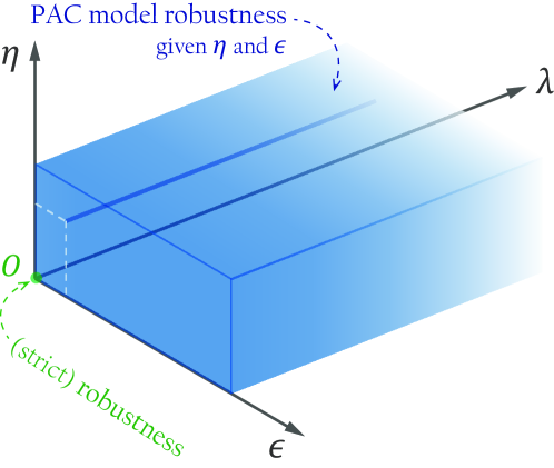
Figure 2. Property space of PAC-model robustness.

4. Methodology

In this section, we present our method for analysing the PAC-model robustness of DNNs. The overall framework is shown in Fig. 3. In general, our method comprises of three stages: sampling, learning, and analysing.

• We sample the input region $B(\hat{\bm{x}},r)$ and obtain the corresponding values of the score difference function $\bm{\Delta}$.

• We learn a PAC model $\widetilde{\bm{\Delta}}(x)\approx_{\eta,\epsilon,\lambda}\bm{\Delta}(x)$ of the score difference function from the samples.

• We analyse whether $\widetilde{\bm{\Delta}}(x)+\lambda$ is always negative in the region $B(\hat{\bm{x}},r)$ by computing its maximal values.

From the description above, we see it is a black-box method since we only use the samples in the neighbour and their corresponding outputs to construct the PAC model. The number of samples is independent of the structure and the size of original models, which will bring the good scalability and efficiency. Moreover, we are essentially reconstructing a proper model to depict the local behavior of the original model. Compared with the statistical methods, the PAC model can potentially extract more information from the score differences of these samples, which supports us to obtain more accurate results.

Note that our framework is constructive, and the PAC model and its maximal points in the region will be constructed explicitly during the analysis. Then, we can obtain the maximal values of the PAC model, and infer that the original DNN satisfies the PAC-model robustness when all maximal values are negative. Thus, DeepPAC can be considered as a sound approach to verify the PAC-model robustness.

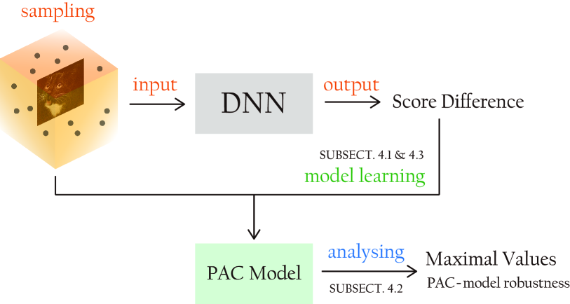
Figure 3. Framework of PAC-model robustness analysis base on model learning

4.1. Learning a PAC Model

To obtain a PAC model of the original score difference function $\bm{\Delta({\bm{x}})}$, we first create a function template, and then determine its parameters by model learning from the samples. Hereafter, we set $\mathcal{F}$ to be the set of affine functions, and consider the PAC model $\widetilde{\bm{\Delta}}(\bm{x})$ to be an affine function with bounded coefficients. A reason for choosing an affine template is that the behaviours of a DNN in a small $L^{\infty}$-norm ball $B(\hat{\bm{x}},r)$ are very similar to some affine function (Ribeiro et al., 2016), due to the almost everywhere differentiability of DNNs. In other words, an affine function can approximate the original model well enough in most cases to maintain the accuracy of our robustness analysis. Specifically, for the $i$th dimension of the DNN output layer, we set $\widetilde{\Delta}_{i}(\bm{x})=\bm{c}_{i}^{\top}\bm{x}=c_{i,0}+c_{i,1}x_{1}+\cdots+c_{i,m}x_{m}$. With extracting a set of $K$ independent and identically distributed samples $\hat{X}\subseteq B(\hat{\bm{x}},r)$, we construct the following optimisation problem for learning the affine PAC model $\widetilde{\bm{\Delta}}(\bm{x})$.

(8) $$\begin{array}[]{lll}&\min\limits_{\lambda\geq 0}\lambda\\ \text{s.t.}&-\lambda\leq\bm{c}_{i}^{\top}\bm{x}-\Delta_{i}(\bm{x})\leq\lambda,&\forall\bm{x}\in\hat{X},\;i\neq\ell\;,\\ &L\leq c_{i,k}\leq U,&i\neq\ell,k=0,\ldots,m\;.\end{array}$$

In the above formulation of PAC model learning, the problem boils down to a linear programming (LP) optimisation. We reuse $\lambda$ to denote the optimal solution, and $\widetilde{\Delta}_{i}$ to be the function whose coefficients $\bm{c}_{i}$ are instantiated according to the optimal solution $\lambda$. Specifically, we aim to compute a PAC model $\widetilde{\bm{\Delta}}$ of $\bm{\Delta}$. By Theorem 2.5, the confidence and the error rate can be ensured by a sufficiently large number of samples. Namely, to make (6) hold with confidence $1-\eta$, we can choose any $K\geq\frac{2}{\epsilon}(\ln\frac{1}{\eta}+(m+1)(n-1)+1)$ corresponding to the number of the variables in (8).

For fixed $\eta$ and $\epsilon$, the number of samples $K$ is in $O(mn)$, so the LP problem (8) contains $O(mn)$ variables and $O(mn^{2})$ constraints. Therefore, the computational cost of the above LP-based approach can quickly become prohibitive with increasing the dimension of input and output.

Example 4.1.

For the MNIST dataset there is the input dimension $m=28$$\times$$28=784$ and output dimension $n=10$. Even for $\eta=0.001,\epsilon=0.4$, we need to solve an LP problem with $7,065$ variables and more than $630,000$ constraints, which takes up too much space (memory out with $10$GB memory).

To further make the PAC model learning scale better with high-dimensional input and output, we will consider several optimisations to reduce the complexity of the LP problem in Section 4.3.

From the LP formulation in Eq. (8), it can be seen that the PAC model learning is based on the sampling set $\hat{X}$ instead of the norm ball $B(\hat{\bm{x}},r)$. That is, though in this paper, for simplicity, $B(\hat{\bm{x}},r)$ is assumed to be an $L^{\infty}$-norm ball, our method also works with $L^{p}$-norm robustness with $1\leq p<\infty$.

4.2. Analysing the PAC Model

We just detailed how to synthesise a PAC model $\widetilde{\bm{\Delta}}$ of the score difference function $\bm{\Delta}$. When the optimisation problem in (8) is solved, we obtain the PAC model $\widetilde{\bm{\Delta}}(x)\approx_{\eta,\epsilon,\lambda}\bm{\Delta}(x)$ of the score difference function. Namely, $\widetilde{\bm{\Delta}}(\bm{x})\pm\lambda$ approximates the upper/lower bound of the score difference function $\bm{\Delta}$ with the PAC guarantee respectively. As aforementioned, all maximal values of $\widetilde{\bm{\Delta}}+\lambda$ being negative implies the PAC-model robustness of the original DNN. According to the monotonicity of affine functions, it is not hard to compute the maximum point $\breve{\bm{x}}^{(i)}$ of $\widetilde{\Delta}_{i}(\bm{x})$ in the region $B(\hat{\bm{x}},r)$. Specifically, for $\widetilde{\Delta}_{i}(\bm{x})$ in the form of $c_{0}+\sum_{j=1}^{m}c_{j}x_{j}$, we can infer its maximum point directly as

$$\breve{\bm{x}}^{(i)}_{j}=\left\{\begin{aligned} &{\hat{\bm{x}}}_{j}+r,\qquad&{{c}}_{j}>0,\\ &{\hat{\bm{x}}}_{j}-r,\qquad&{{c}}_{j}\leq 0.\end{aligned}\right.$$

Note that the choice of $\breve{\bm{x}}^{(i)}_{j}$ is arbitrary for the case $c_{j}=0$. Here, we choose ${\hat{\bm{x}}}_{j}-r$ as an instance. Then let $\breve{\bm{x}}$ be the $\breve{\bm{x}}^{(i)}$ corresponding to the maximum $\widetilde{{\Delta}}_{i}(\breve{\bm{x}}^{(i)})$, and the PAC-model robustness of the original DNN immediately follows if $\widetilde{\Delta}(\breve{\bm{x}})+\lambda<\bm{0}$. Besides, each $\breve{\bm{x}}^{(i)}$ is a potential adversarial example attacking the original DNN with the classification label $i$, which can be further validated by checking the sign of $\Delta_{i}(\breve{\bm{x}}^{(i)})$.

Example 4.2.

We consider the neural network in Fig. 1. Given an input $\hat{\bm{x}}=(0,0)^{\top}$, the classification label is $C_{\bm{f}}(\hat{\bm{x}})=1$. The network is robust if $f_{2}(\bm{x})<f_{1}(\bm{x})$ for $\bm{x}\in B(\hat{\bm{x}},1)$, or equivalently, $f_{2}(\bm{x})-f_{1}(\bm{x})<0$. Thus, our goal is to apply the scenario approach to learn the score difference $\Delta(\bm{x})=f_{2}(\bm{x})-f_{1}(\bm{x})$. In this example, we take the approximating function of the form $\widetilde{\Delta}(\bm{x})=c_{0}+c_{1}x_{1}+c_{2}x_{2}$ with constant parameters $c_{0},c_{1},c_{2}\in[-100,100]$ to be synthesised. For ease of exposition, we denote $\bm{c}=(c_{1},c_{2},c_{3})^{\top}$.

We attempt to approximate $\Delta(\bm{x})$ by minimising the absolute difference between it and the approximating function $\widetilde{\Delta}(\bm{x})$. This process can be characterised as an optimisation problem:

(9) $$\begin{array}[]{lll}&\min\limits_{\bm{c},\lambda}\lambda&\\ \mathrm{s.t.}&|\widetilde{\Delta}(\bm{x})-\Delta(\bm{x})|\leq\lambda,&\forall\bm{x}\in[-1,1]^{2}\;,\\ &\bm{c}\in[-100,100]^{3},&\\ &\lambda\in[-100,100]\;.&\end{array}$$

To apply the scenario approach, we first need to extract a set of $K$ independent and identically distributed samples $\hat{X}\subseteq[-1,1]^{2}$, and then reduce the optimisation problem (9) to the linear programming problem by replacing the quantifier $\forall\bm{x}\in[-1,1]^{2}$ with $\forall\bm{x}\in\hat{X}$ in the constraints. Theorem 2.5 indicates that at least $\lceil\frac{2}{\epsilon}(\ln\frac{1}{\eta}+4)\rceil$ samples are required to guarantee the error rate within $\epsilon$, i.e. $\mathbb{P}(|\widetilde{\Delta}(\bm{x})-\Delta(\bm{x})|\leq\lambda)\geq 1-\epsilon$, with confidence $1-\eta$.

Taking the error rate $\epsilon=0.01$ and the confidence $1-\eta=99.9\%$, we need (at least) $K=2182$ samples in $[-1,1]^{2}$. By solving the resulting linear program again, we obtain $c_{0}=-22.4051$, $c_{1}=2.800$, $c_{2}=-9.095$, and $\lambda=9.821$.

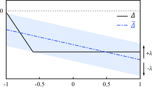
Figure 4. The functions $\Delta$ and $\widetilde{\Delta}$ in $x_{2}$ are depicted by fixing $x_{1}=1$. It is marked red where $\Delta(\bm{x})$ is not bounded by $\widetilde{\Delta}(\bm{x})\pm\lambda$.

For illustration, we restrict $x_{1}=1$, and depict the functions $\Delta$ and $\widetilde{\Delta}$ in Fig. 4. Our goal is to verify that the first output is always larger than the second, i.e., $\Delta(\bm{x})=f_{2}(\bm{x})-f_{1}(\bm{x})<0$. As described above, according to the signs of the coefficients of $\widetilde{\Delta}$, we obtain that $\widetilde{\Delta}(\bm{x})$ attains the maximum value at $\bm{x}=(1,-1)^{\top}$ in $[-1,1]^{2}$. Therefore, the network is PAC-model robustness.

4.3. Strategies for Practical Analysis

We regard efficiency and scalability as the key factor for achieving practical analysis of DNN robustness. In the following, we propose three practical PAC-model robustness analysis techniques.

4.3.1. Component-based learning

As stated in Section 4.1, the complexity of solving (8) can still be high, so we propose component-based learning to reduce the complexity. As before, we use $\widetilde{\Delta}_{i}$ to approximate $\Delta_{i}(\bm{x})=f_{i}(\bm{x})-f_{\ell}(\bm{x})$ for each $i$ with the same template. The idea is to learn the functions $\Delta_{1},\ldots,\Delta_{n}$ separately, and then combine the solutions together. Instead of solving a single large LP problem, we deal with $(n-1)$ individual smaller LP problems, each with $O(m)$ linear constraints. As a result, we have $\widetilde{\Delta}_{i}(\bm{x})\approx_{\eta,\epsilon,\lambda_{i}}\Delta_{i}(\bm{x})$, from which we can only deduce that

$$\mathbb{P}\Big{(}\bigwedge_{i\neq\ell}|\widetilde{\Delta}_{i}(\bm{x})-\Delta_{i}(\bm{x})|\leq\lambda_{i}\Big{)}\geq 1-(n-1)\epsilon$$

with the confidence decreasing to at most $1-(n-1)\eta$. To guarantee the error rate at least $\epsilon$ and the confidence at least $1-\eta$, we need to recompute the error $\lambda$ between $\widetilde{\bm{\Delta}}(\bm{x})$ and $\bm{\Delta}(\bm{x})$. Specifically, we solve the following optimisation problem constructed by resampling:

(10) $$\begin{array}[]{lll}&\min\limits_{\lambda}\lambda&\\ \text{s.t.}&|\widetilde{\Delta}_{i}(\bm{x})-\Delta_{i}(\bm{x})|\leq\lambda,\\ &\forall\bm{x}\in\hat{X}\;,i\neq\ell.\end{array}$$

where $\hat{X}$ is a set of $K$ i.i.d samples with $K\geq\tfrac{2}{\epsilon}(\ln\tfrac{1}{\eta}+1)$. Applying Theorem 2.5 again, we have $\widetilde{\bm{\Delta}}(\bm{x})\approx_{\eta,\epsilon,\lambda}\bm{\Delta}(\bm{x})$ as desired.

We have already relaxed the optimisation problem (8) into a family of $(n-1)$ small-scale LP problems. If $n$ is too large (e.g. for Imagenet with $1000$ classes), we can also consider the untargeted score difference function ${\Delta}_{\mathrm{u}}(\bm{x})=\bm{f}_{\ell}(\bm{x})-\max_{i\neq l}\bm{f}_{i}(\bm{x})$. By adopting the untargeted score difference function, the number of the LP problems is reduced to one. The untargeted score difference function improves the efficiency at expense of the loss of linearity, which harms the accuracy of the affine model.

4.3.2. Focused learning

In this part, our goal is to reduce the complexity further by dividing the learning procedure into two phases with different fineness: i) in the first phase, we use a small set of samples to extract coefficients with big absolute values; and ii) these coefficients are “focused” in the second phase, in which we use more samples to refine them. In this way, we reduce the number of variables overall, and we call it focused learning, which namely refers to focusing the model learning procedure on important features. It is embedded in the component learning procedure.

The main idea of focused learning is depicted below:

1. First learning phase: We extract $K^{(1)}$ i.i.d. samples from the input region $B(\hat{\bm{x}},r)$. We first learn $\Delta_{i}$ on the $K^{(1)}$ samples. Thus, our LP problems have $O(K^{(1)})$ constraints with $O(m)$ variables. For large datasets like ImageNet, the resulting LP problem is still too large. We use efficient learning algorithms such as linear regression (ordinary least squares) to boost the first learning phase on these large datasets.

2. Key feature extraction: After solving the LP problem (or the linear regression for large datasets), we synthesise $\widetilde{\Delta}_{i}^{(1)}$ as the approximating function. Let $\mathit{KeyF}_{i}(\kappa)\subseteq\{1,x_{1},\ldots,x_{m}\}$ denote the set of extracted key features for the $i$th component corresponding to the $\kappa$ coefficients with the largest absolute values in $\widetilde{\Delta}_{i}^{(1)}$.

3. Focused learning phase: We extract $K^{(2)}$ i.i.d. samples from $B(\hat{\bm{x}},r)$. For these samples, we generate constraints only for our key features in $\mathit{KeyF}_{i}(\kappa)$ by fixing the other coefficients using those in $\widetilde{\Delta}_{i}^{(1)}$, and thus the number of the undetermined coefficients is bounded by $\kappa$. By solving an LP problem comprised of these constraints, we finally determine the coefficients of the features in $\mathit{KeyF}_{i}(\kappa)$.

We can determine the sample size $K^{(2)}$ and the number of key features $\kappa$ satisfying

$$\kappa\leq\frac{K^{(2)}\epsilon}{2}-\ln\frac{1}{\eta}-1\;,$$

which can be easily inferred from Theorem 2.5. It is worth mentioning that, focused learning not only significantly improves the efficiency, but it also makes our approach insensitive to significance level $\eta$ and error rate $\epsilon$, because the first phase in focused learning can provide a highly precise model, and a small number of samples are sufficient to learn the PAC model in the second phase. This will be validated in our experiments.

4.3.3. Stepwise splitting

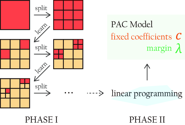
Figure 5. A workflow of the stepwise splitting procedure. The red color indicates the significant grids whose coefficients will be further refined, while the yellow color indicates the grids whose coefficients have been determined.

When the dimensionality of the input space is very high (e.g., ImageNet), The first learning phase of focused learning requires constraints generated by tons of samples to make precise predictions on the key features, which is very hard and even impossible to be directly solved. For achieving better scalability, we partition the dimensions of input $\{1,\ldots,m\}$ into groups $\{G_{k}\}$. In an affine model $\widetilde{\Delta}_{i}$, for the variables with undetermined coefficients in each certain group $G_{k}$, they share the same coefficient $c_{k}$. Namely, the affine model has the form of $\sum_{k}\left(c_{k}\sum_{i\in G_{k}}x_{i}\right)$. Then, a coarse model can be learned.

We compose the refinement into the procedure of focused learning aforementioned (See Fig. 5). Specifically, after a coarse model is learned, we fix the coefficients for the insignificant groups and extract the key groups. The key groups are then further refined, and their coefficients are renewed by learning on a new batch of samples. We repeat this procedure iteratively until most coefficients of the affine model are fixed, and then we invoke linear programming to compute the rest coefficients and the margin. This iterative refinement can be regarded as multi-stage focused learning with different fineness.

In particular, for a colour image, we can use the grid to divide its pixels into groups. The image has three channels corresponding to the red, green and blue levels. As a result, each grid will generate 3 groups matching these channels, i.e. $G_{k,\mathrm{R}}$, $G_{k,\mathrm{G}}$, and $G_{k,\mathrm{B}}$. Here, we determine the significance of a grid with the $L^{2}$-norm of the coefficients of its groups, i.e. $(c_{k,\mathrm{R}}^{2}+c_{k,\mathrm{G}}^{2}+c_{k,\mathrm{B}}^{2})^{\frac{1}{2}}$. Then the key groups (saying corresponding to the top $25\%$ significant grids) will be further refined in the subsequent procedure. On ImageNet, we initially divide the image into $32\times 32$ grids, with each grid of the size $7\times 7$. In each refinement iteration, we split each significant grid into 4 sub-grids (see Fig. 5). We perform 6 iterations of such refinement and use $20\,000$ samples in each iteration. An example on stepwise splitting of an ImageNet image can be found in Fig. 8 in Sect. 5.3.

5. Experimental EVALUATION

In this section, we evaluate our PAC-model robustness verification method. We implement our algorithm as a prototype called DeepPAC. Its implementation is based on Python 3.7.8. We use CVXPY (Diamond and Boyd, 2016) as the modeling language for linear programming and GUROBI (Gurobi Optimization, 2021) as the LP solver. Experiments are conducted on a Windows 10 PC with Intel i7 8700, GTX 1660Ti, and 16G RAM. Three datasets MNIST (Lécun et al., 1998), CIFAR-10 (Krizhevsky et al., 2009), and ImageNet (Russakovsky et al., 2015) and 20 DNN models trained from them are used in the evaluation. The details are in Tab. 1. We invoke our component-based learning and focused learning for all evaluations, and apply stepwise splitting for the experiment on ImageNet. All the implementation and data used in this section are publicly available.

In the following, we are going to answer the research questions below.

• Can DeepPAC evaluate local robustness of a DNN more effectively compared with the state-of-the-art?

• Can DeepPAC retain a reasonable accuracy with higher significance, higher error rate, and/or fewer samples?

• Is DeepPAC scalable to DNNs with complex structure and high dimensional input?

• Is there a underlying relation between DNN local robustness verification and DNN testing (especially the test selection)?

Dataset	Network	Defense	#Param	Source
MNIST	FNN1	—	44.86 K	—
	FNN2		99.71 K
	FNN3		239.41 K
	FNN4		360.01 K
	FNN5		480.61 K
	FNN6		1.65 M
	CNN1	—	89.61 K	ERAN
	CNN2	DiffAI
	CNN3	PGD
	CNN4	—	1.59 M
	CNN5	PGD, $\varepsilon=0.1$
	CNN6	PGD, $\varepsilon=0.3$
CIFAR-10	CNN1	PGD	125.32 K
	CNN2	PGD, $\varepsilon=2/255$	2.07 M
	CNN3	PGD, $\varepsilon=8/255$
	ResNet18		11.17 M	—
	ResNet50		23.52 M
	ResNet152		58.16 M
ImageNet	ResNet50a	PGD, $\varepsilon=4/255$	25.56 M	Madry
	ResNet50b	PGD, $\varepsilon=8/255$

Table 1. Datasets and DNNs used in our evaluation. The convolutional neural networks (CNN) for MNIST and CIFAR-10 are from ERAN (SRI Lab, 2020). The ResNet50 networks for ImageNet are from the python library “Robustness” (Engstrom et al., 2019) produced by MadryLab. The rest networks are trained by ourselves.

5.1. Comparison on Precision

Figure 6. Each dash represents the maximum robustness radius for an input estimated by DeepPAC (blue) or PROVERO (red), while each bar (white) gives an interval containing the exact maximum robustness radius, whose lower bound and upper bound are computed by ERAN and PGD, respectively.

We first apply DeepPAC for evaluating DNN local robustness by computing the maximum robustness radius and compare DeepPAC with the state-of-the-art statistical verification tool PROVERO (Baluta et al., 2021), which verifies PAC robustness by statistical hypothesis testing. A DNN verification tool returns true or false for robustness of a DNN given a specified radius value. A binary search will be conducted for finding the maximum robustness radius. For both DeepPAC and PROVERO, we set the error rate $\epsilon=0.01$ and the significance level $\eta=0.001$. We set $K^{(1)}=2000$ and $K^{(2)}=8000$ for DeepPAC.

In addition, we apply ERAN (Singh et al., 2019) and PGD (Madry et al., 2018) to bound the exact maximum radius from below and from above, respectively. ERAN is a state-of-the-art DNN formal verification tool based on abstract interpretation, and PGD is a popular adversarial attack algorithm. In the experiments, we use the PGD implementation from the commonly used Foolbox (Rauber et al., 2017) with $40$ iterations and a relative step size of $0.033$, which are suggested by Foolbox as a default setting. Note that exact robustness verification SMT tools like Marabou (Katz et al., 2019) cannot scale to the benchmarks used in our experiment.

We run all the tools on the first 12 DNN models in Tab. 1 and the detailed results are recorded in Fig. 6. In all cases, the maximum robustness radius estimated by the PROVERO is far larger than those computed by other tools. In most cases, PROVERO ends up with a maximum robustness radius over $100$ (out of 255), which is even larger than the upper bound identified by PGD. This indicates that, while a DNN is proved to be PAC robust by PROVERO, adversarial inputs can be still rather easily found within the verified bound. In contrast, DeepPAC estimates the maximum robustness radius more accurately, which falls in between the results from ERAN and PGD mostly. Since the range between the estimation of ERAN and PGD contains the exact maximum robustness radius, we conclude that DeepPAC is a more accurate tool than PROVERO to analyse local robustness of DNNs.

DeepPAC also successfully distinguishes robust DNN models from non-robust ones. It tells that the CNNs, especially the ones with defence mechanisms, are more robust against adversarial perturbations. For instance, 24 out of 25 images have a larger maximum robustness radius on CNN1 than on FNN1, and 21 images have a larger maximum robustness radius on CNN2 than on CNN1.

Other than the maximum robustness radius for a fixed input, the overall robustness of a DNN, subject to some radius value, can be denoted by the rate of the inputs being robust in a dataset, called “robustness rate”. In Fig. 7, we show the robustness rate of 100 input images estimated by different tools on the 3 CIFAR-10 CNNs. Here, we set $K^{(1)}=20\,000$ and $K^{(2)}=10\,000$.

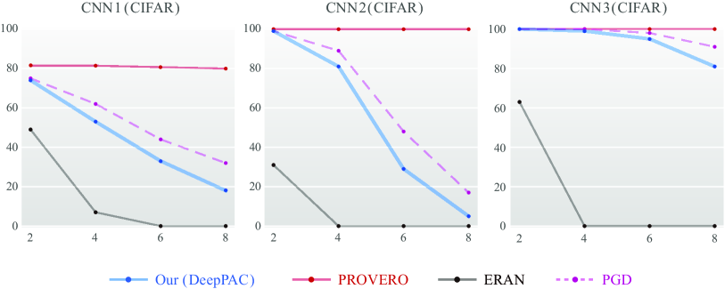
Figure 7. Robustness rate of different CNNs under the radius of 2, 4, 6, and 8 on CIFAR-10.

PROVERO, similarly to the earlier experiment outcome, results in robustness rate which is even higher than the upper bound estimation from the PGD attack, and its robustness rate result hardly changes when the robustness radius increases. All such comparisons reveal the limitations of using PAC robustness (by PROVERO) that the verified results are not tight enough.

ERAN is a sound verification method, and the robustness rate verified by it is a strict lower bound of the exact result. However, this lower bound could be too conservative and ERAN quickly becomes not usable. In the experiments, we find that it is hard for ERAN to verify a robustness radius greater than or equal to 4 (out of 255).

DeepPAC verifies greater robustness rate and larger robustness radius, with high confidence and low error rate. Its results fall safely into the range bounded by ERAN and PGD. We advocate DeepPAC as a more practical DNN robustness analysis technique. It is shown in our experiments that, though DeepPAC does not enforce 100% guarantee, it can be applied into a wider range of adversarial settings (in contrast to ERAN) and the PAC-model verification results by DeepPAC can be more trusted (in contrast to PROVERO) with quantified confidence (in contrast to PGD).

Answer RQ1: The maximum robustness radius estimated by DeepPAC is more precise than that by PROVERO, and our DeepPAC is a more practical DNN robustness analysis method.

5.2. DeepPAC with Different Parameters

In this part, we experiment on the three key parameters in DeepPAC: the error rate $\epsilon$, the significance level $\eta$, and the number of samples $K^{(1)}$ in the first learning phase. The parameters $\eta$ and $\epsilon$ control the precision between the PAC model and the original model. The number of samples $K^{(1)}$ determines the accuracy of the first learning phase. We evaluate DeepPAC under different parameters to check the variation of the maximal robustness radius. We set either $K^{(1)}=20000$ or $K^{(1)}=5000$ in our evaluation and three combinations of the parameters $(\epsilon,\eta)$: $(0.01,0.001)$, $(0.1,0.001)$, and $(0.01,0.1)$. Here, we fix the number of key features to be fifty, i.e. $\kappa=50$, and calculate the corresponding number of samples $K^{(2)}$ in the focused learning phase.

The results are presented in Tab. 2. DeepPAC reveals some DNN robustness insights that were not achievable by other verification work. It is shown that, the DNNs (the ResNet family experimented) can be more robust than many may think. The maximum robustness radius remains the same or slightly alters, along with the error rate $\eta$ and significance level $\epsilon$ varying. This observation also confirms that the affine model used in DeepPAC abstraction converges well, and the resulting error bound is even smaller than the specified (large) error bound. Please refer to Sect. 4.1 for more details.

DeepPAC is also tolerant enough with a small sampling size. When the number of samples in the first learning phase decreases from $K^{(1)}=20,000$ to $K^{(1)}=5,000$, we can observe a minor decrease of the maximal robustness radius estimation. Recall that we utilise the learned model in the first phase of focused learning to extract the key features and provide coefficients to the less important features. When the sampling number decreases, the learned model would be less precise and thus make vague predictions on key features and make the resulting affine model shift from the original model. As a result, the maximum robustness radius can be smaller when we reduce the number of sampling in the first phase. In practice, as it is shown by the results in Tab. 2, we do not observe a sudden drop of the DeepPAC results when using a much smaller sampling size.

Input Image	Network	$\eta,\epsilon$ and $K^{(1)}$
		$0.01,0.001$		$0.1,0.001$		$0.01,0.1$
		20K	5K	20K	5K	20K	5K
	ResNet18	5	4	5	4	5	4
	ResNet50	8	8	8	8	9	8
	ResNet152	5	5	5	5	5	5
	ResNet18	16	14	15	14	15	14
	ResNet50	12	11	12	12	12	11
	ResNet152	10	9	10	9	10	9
	ResNet18	11	10	11	10	11	10
	ResNet50	6	5	6	5	6	5
	ResNet152	9	8	9	8	9	8
	ResNet18	1	1	1	1	1	1
	ResNet50	3	3	3	3	3	3
	ResNet152	6	5	6	5	6	5
	ResNet18	16	13	16	14	16	14
	ResNet50	17	15	17	15	17	15
	ResNet152	12	10	12	10	12	10

Table 2. The maximum robustness radius estimated by DeepPAC on CIFAR-10 dataset using different parameters, i.e. significance level $\eta$, error rate $\epsilon$, and the number of samples in the first learning phase $K^{(1)}$.

Answer RQ2: DeepPAC shows good tolerance to different configurations of its parameters such as the error rate $\epsilon$, the significance level $\eta$, and the number of samples $K^{(1)}$.

5.3. Scalability

Robustness verification is a well-known difficult problem on complex networks with high-dimensional data. Most qualitative verification methods meet a bottleneck in the size and structure of the DNN. The fastest abstract domain in ERAN is GPUPoly (Müller et al., 2020), a GPU accelerated version of DeepPoly. The GPUPoly can verify a ResNet18 model on the CIFAR-10 dataset with an average time of 1 021 seconds under the support of an Nvidia Tesla V100 GPU. To the best of our knowledge, ERAN does not support models on ImageNet, which makes it limited in real-life scenarios. The statistical methods alleviate this dilemma and extend their use further. The state-of-the-art PAC robustness verifier PROVERO needs to draw 737 297 samples for VGG16 and 722 979 samples for VGG19 on average for each verification case on ImageNet. The average running time is near 2208.9 seconds and 2168.9 seconds (0.003 seconds per sample) under the support of an Nvidia Tesla V100 GPU. We will show that DeepPAC can verify the tighter PAC-model robustness on ImageNet with less samples and time on much larger ResNet50 models.

In this experiment, we apply DeepPAC to the start-of-the-art DNN with high resolution ImageNet images. The two ResNet50 networks are from the python package named “robustness” (Engstrom et al., 2019). We check PAC-model robustness of the two DNNs with the same radius $4$ (out of $255$). The first evaluation is on a subset of ImageNet images from 10 classes (Howard, 2019). The second one includes ImageNet images of all 1,000 classes and the untargeted score difference function is configured for DeepPAC. To deal with ImageNet, the stepwise splitting mechanism in Sect. 4.3.3 is adopted. An illustrating example of the stepwise splitting is given in Fig. 8. As we expect, the splitting refinement procedure successfully identifies the significant features of a golf ball, i.e. the boundary and the logo. It maintains the accuracy of the learned model with much less running time. The results are shown in Tab. 3.

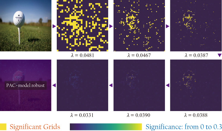
Figure 8. Stepwise splitting procedures of DeepPAC, illustrated by heatmaps of grid significance. Top 25% significant grids are colored yellow in the heatmap, which is split and refined iteratively. The margin $\lambda$ of different refinement stage is under the heatmap.

For the 10-class setup, we evaluate the PAC-model robustness on 50 images and it takes less than 1800 seconds on each case. DeepPAC finds out 30 and 29 cases PAC-model robust for ResNet50a and ResNet50b, respectively. Because the two models have been defensed, when we perform the PGD attack, only one adversarial examples were found for each model, which means that PGD gives no conclusion for the robustness evaluation on most cases under this setting. For the 1000-class dataset, the untargeted version of DeepPAC has even better efficiency with the running time of less than 800 seconds each, which mainly benefits from reducing the score difference function to the untargeted one. DeepPAC proves 10 and 6 out of 50 cases to be PAC-model robust on the 1000-class setup, respectively. For both setups, DeepPAC uses 121 600 samples to learn a PAC model effectively.

Method	Network	Robust	Min	Max	Avg
Targeted (10 classes)	ResNet50a	30/50	1736.5	1768.8	1751.8
	ResNet50b	29/50	1722.1	1781.5	1746.5
Untargeted (1000 classes)	ResNet50a	10/50	779.2	785.3	781.7
	ResNet50b	6/50	775.7	783.8	778.3

Table 3. The performance of DeepPAC analysing the two ResNet50 models for ImageNet. “Robust” represents the robustness rate. “Min”, “Max”, and “Avg” are the minimum, maximum, and average of the running time (second), respectively.

Answer RQ3: The DeepPAC robustness analysis scales well to complex DNNs with high-dimensional data like ImageNet, which is not achieved by previous formal verification tools. It shows superiority to PROVERO in both running time and the number of samples.

5.4. Relation with Testing Prioritising Metric

We also believe that there is a positive impact from practical DNN verification work like DeepPAC on DNN testing. For example, the tool DeepGini uses Gini index, which measures the confidence of a DNN prediction on the corresponding input, to sort the testing inputs. In Tab. 4, we report the Pearson correlation coefficient between the DeepGini indices and the maximal robustness radii obtained by DeepPAC, ERAN and PROVERO from the experiment in Sect. 5.1.

As in Tab. 4, the maximum robustness radius is correlated to the DeepGini index, a larger absolute value of the coefficient implies a stronger correlation. It reveals the data that has low prediction confidence is also prone to be lack robustness. From this phenomenon, we believe DeepGini can be also helpful in data selection for robustness analysis. Interestingly, the maximum robustness radius computed by our DeepPAC has higher correlations with DeepGini index on the CNNs, which are more complex, than on FNNs. Furthermore, DeepPAC shows the strongest correlation on the CNNs trained with defense mechanisms, while the correlation between PROVERO or ERAN and DeepGini is relatively weak on these networks. Intuitively, complex models with defense are expected to be more robust. Again, we regard this comparison result as the evidence from DNN testing to support the superior of DeepPAC over other DNN verification tools. From the perspective of testing technique, it is promising to combine these two methods for achieving test selection with guarantee.

Network	DeepPAC	ERAN	PROVERO
FNN1	-0.3628	-0.3437	-0.3968
FNN2	-0.4851	-0.4353	-0.5142
FNN3	-0.4174	-0.3677	-0.4223
FNN4	-0.5264	-0.4722	-0.5234
FNN5	-0.4465	-0.6016	-0.5916
FNN6	-0.4538	-0.2747	-0.3949
CNN1	-0.7340	-0.7345	-0.8223
CNN2 $\star$	-0.6482	-0.6478	-0.4527
CNN3 $\star$	-0.7216	-0.6728	-0.5218
CNN4	-0.6035	-0.6127	-0.7771
CNN5 $\star$	-0.7448	-0.6833	-0.3874
CNN6 $\star$	-0.6498	-0.6094	-0.4763

Table 4. The Pearson correlation coefficient between the maximum robustness radius estimation and the DeepGini index. The DNNs are marked by “$\star$” if they are trained with defense mechanisms.

Answer RQ4: The maximum robustness radius estimated by DeepPAC, ERAN, and PROVERO are all correlated to the DeepGini index, where DeepPAC and DeepGini show the strongest correlation on robust models.

5.5. Case Study: Verifying Cloud Service API

To show the practicality of DeepPAC, we apply it to analyse the robustness of black-box models for real-world cloud services. The case we study here is the image recognition API provided by Baidu AI Cloud, which accepts an image and returns a pair list in the form of $(\mathrm{label}_{i},\mathrm{score}_{i})$ to indicate the top classes the input recognised to be. We use the image of a dandelion as the input, which is an official example in its illustration.

By setting $\eta=0.001$ and $\epsilon=0.01$, we verify the PAC-model robustness for its top label “dandelion” within the radius of $5/255$. A total of 49,600 samples are utilised in the whole procedure. By DeepPAC, we obtain the PAC-model of the difference function, but unfortunately, its maximal value in the input $L_{\infty}$ ball is larger than zero. As an intermediate output, we generate a potential adversarial example via the PAC model. By feeding it back into the model, we checked that it is a true adversarial example with “sky” as its top label (see Fig. 9).

An interesting observation is that the labels output by the image recognition API may be not independent. For instance, the class labels “dandelion” and “plant” may appear in the output list at the same time, and both of them can be considered correct labels. Therefore, we believe that in the future new forms of DNN robustness properties also need to be studied e.g., the sum of the output scores for the correct labels (“dandelion” and “plant”) should be larger than some threshold. DeepPAC is a promising tool to cope with these emerging challenges when considering real-world applications of DNN robustness analysis, by conveniently adjusting its difference function.

(a)

(b)

Figure 9. The original image (left) gain the score $(\mathrm{dandelion}:0.758,\mathrm{sky}:0.600)$, and the adversarial example gain the score $(\mathrm{sky}:0.791,\mathrm{dandelion}:0.621)$.

6. Related Work

Here we discuss more results on the verification, adversarial attacks and testing for DNNs. A number of formal verification techniques have been proposed for DNNs, including constraint-solving (Katz et al., 2017; Ehlers, 2017; Narodytska et al., 2018; Bunel et al., 2020; Lin et al., 2019; Gokulanathan et al., 2020; Gopinath et al., 2018; Feng et al., 2018), abstract interpretation (Gehr et al., 2018; Li et al., 2019; Singh et al., 2018; Singh et al., 2019; Yang et al., 2021), layer-by-layer exhaustive search (Huang et al., 2017), global optimisation (Ruan et al., 2018; Dutta et al., 2018; Ruan et al., 2019), convex relaxation (Julian et al., 2019; Paulsen et al., 2020a, b), functional approximation (Weng et al., 2018), reduction to two-player games (Wicker et al., 2018; Wu et al., 2020), and star-set-based abstraction (Tran et al., 2019; Tran et al., 2020a). Sampling-based methods are adopted to probabilistic robustness verification in (Webb et al., 2019; Weng et al., 2019; Mangal et al., 2019b; Cardelli et al., 2019a; Anderson and Sojoudi, 2020a, b). Most of them provide sound DNN robustness estimation in the form of a norm ball, but typically for very small networks or with pessimistic estimation of the norm ball radius. By contrast, statistical methods (Webb et al., 2019; Weng et al., 2019; Baluta et al., 2021; Mangal et al., 2019a; Wicker et al., 2020; Baluta et al., 2019; Cardelli et al., 2019b; Huang et al., 2021) are more efficient and scalable when the structure of DNNs is complex. The primary difference between these methods and DeepPAC is that our method is model-based and thus more accurate. We use samples to learn a relatively simple model of the DNN with the PAC guarantee via scenario optimisation and gain more insights to the analysis of adversarial robustness. The generation of adversarial inputs (Szegedy et al., 2014) itself has been widely studied by a rich literature of adversarial attack methods. Some most well-known robustness attack methods include Fast Gradient Sign (Goodfellow et al., 2015), Jacobian-based saliency map approach (Papernot et al., 2016), C&W attack (Carlini and Wagner, 2017), etc. Though adversarial attack methods generate adversarial inputs efficiently, they cannot enforce guarantee of any form for the DNN robustness. Testing is still the primary approach for certifying the use of software products and services. In recent years, significant work has been done for the testing for DNNs such as test coverage criteria specialised for DNNS (Pei et al., 2017; Ma et al., 2018a; Sun et al., 2019; Kim et al., 2019; Yan et al., 2020) and different testing techniques adopted for DNNs (Tian et al., 2018; Zhang et al., 2018; Xie et al., 2019; Ma et al., 2018c; Sun et al., 2020; Wang et al., 2021a; Humbatova et al., 2021; Riccio and Tonella, 2020; Ma et al., 2018b; Yan et al., 2021). In particular, our experiments show that the results from DeepPAC are consistent with the DNN testing work for prioritising test inputs (Feng et al., 2020; Wang et al., 2021b), but with a stronger guarantee. This highlights again that DeepPAC is a practical verification method for DNN robustness.

7. Conclusion and Future Work

We propose DeepPAC, a method based on model learning to analyse the PAC-model robustness of DNNs in a local region. With the scenario optimisation technique, we learn a PAC model which approximates the DNN within a uniformly bounded margin with a PAC guarantee. With the learned PAC model, we can verify PAC-model robustness properties under specified confidence and error rate. Experimental results confirm that DeepPAC scales well on large networks, and is suitable for practical DNN verification tasks. As for future work, we plan to learn more complex PAC models rather than the simple affine models, and we are particularly interested in exploring the combination of practical DNN verification by DeepPAC and DNN testing methods following the preliminary results.

References

- (1)
- Alzantot et al. (2019) Moustafa Alzantot, Yash Sharma, Supriyo Chakraborty, Huan Zhang, Cho-Jui Hsieh, and Mani B. Srivastava. 2019. GenAttack: practical black-box attacks with gradient-free optimization. In GECCO 2019, Anne Auger and Thomas Stützle (Eds.). ACM, Prague, Czech Republic, 1111–1119.
- Anderson and Sojoudi (2020a) Brendon G. Anderson and Somayeh Sojoudi. 2020a. Certifying Neural Network Robustness to Random Input Noise from Samples. arXiv:2010.07532 [cs.LG]
- Anderson and Sojoudi (2020b) Brendon G. Anderson and Somayeh Sojoudi. 2020b. Data-Driven Assessment of Deep Neural Networks with Random Input Uncertainty. arXiv:2010.01171 [cs.LG]
- Ashok et al. (2020) Pranav Ashok, Vahid Hashemi, Jan Kretínský, and Stefanie Mohr. 2020. DeepAbstract: Neural Network Abstraction for Accelerating Verification. In ATVA 2020 (Lecture Notes in Computer Science, Vol. 12302), Dang Van Hung and Oleg Sokolsky (Eds.). Springer, 92–107.
- Baluta et al. (2021) Teodora Baluta, Zheng Leong Chua, Kuldeep S Meel, and Prateek Saxena. 2021. Scalable quantitative verification for deep neural networks. In ICSE 2021. IEEE, Madrid, Spain, 312–323.
- Baluta et al. (2019) Teodora Baluta, Shiqi Shen, Shweta Shinde, Kuldeep S. Meel, and Prateek Saxena. 2019. Quantitative Verification of Neural Networks and Its Security Applications. In CCS 2019, November 11-15, 2019, Lorenzo Cavallaro, Johannes Kinder, XiaoFeng Wang, and Jonathan Katz (Eds.). ACM, London, UK, 1249–1264.
- Boopathy et al. (2019) Akhilan Boopathy, Tsui-Wei Weng, Pin-Yu Chen, Sijia Liu, and Luca Daniel. 2019. CNN-Cert: An Efficient Framework for Certifying Robustness of Convolutional Neural Networks. In AAAI 2019, January 27 - February 1, 2019. AAAI Press, Honolulu, Hawaii, USA, 3240–3247.
- Bunel et al. (2020) Rudy Bunel, Jingyue Lu, Ilker Turkaslan, Philip H. S. Torr, Pushmeet Kohli, and M. Pawan Kumar. 2020. Branch and Bound for Piecewise Linear Neural Network Verification. J. Mach. Learn. Res. 21 (2020), 42:1–42:39.
- Calafiore and Campi (2006) Giuseppe Carlo Calafiore and Marco C. Campi. 2006. The scenario approach to robust control design. IEEE Trans. Autom. Control. 51, 5 (2006), 742–753.
- Campi et al. (2009) Marco C. Campi, Simone Garatti, and Maria Prandini. 2009. The scenario approach for systems and control design. Annu. Rev. Control. 33, 2 (2009), 149–157.
- Cardelli et al. (2019b) Luca Cardelli, Marta Kwiatkowska, Luca Laurenti, Nicola Paoletti, Andrea Patane, and Matthew Wicker. 2019b. Statistical Guarantees for the Robustness of Bayesian Neural Networks. In IJCAI 2019, August 10-16, 2019, Sarit Kraus (Ed.). ijcai.org, Macao, China, 5693–5700.
- Cardelli et al. (2019a) Luca Cardelli, Marta Kwiatkowska, Luca Laurenti, and Andrea Patane. 2019a. Robustness Guarantees for Bayesian Inference with Gaussian Processes. In AAAI 2019, January 27 - February 1, 2019. AAAI Press, Honolulu, Hawaii, USA, 7759–7768.
- Carlini and Wagner (2017) Nicholas Carlini and David Wagner. 2017. Towards evaluating the robustness of neural networks. In S&P 2017. IEEE, IEEE Computer Society, San Jose, CA, USA, 39–57.
- Diamond and Boyd (2016) Steven Diamond and Stephen Boyd. 2016. CVXPY: A Python-embedded modeling language for convex optimization. Journal of Machine Learning Research 17, 83 (2016), 1–5.
- Dutta et al. (2018) Souradeep Dutta, Susmit Jha, Sriram Sankaranarayanan, and Ashish Tiwari. 2018. Output Range Analysis for Deep Feedforward Neural Networks. In NFM 2018 (Lecture Notes in Computer Science, Vol. 10811), Aaron Dutle, César A. Muñoz, and Anthony Narkawicz (Eds.). Springer, Newport News, VA, USA, 121–138.
- Ehlers (2017) Rüdiger Ehlers. 2017. Formal Verification of Piece-Wise Linear Feed-Forward Neural Networks. In ATVA 2017. Springer, Pune, India, 269–286.
- Elboher et al. (2020) Yizhak Yisrael Elboher, Justin Gottschlich, and Guy Katz. 2020. An Abstraction-Based Framework for Neural Network Verification. In CAV 2020 (Lecture Notes in Computer Science, Vol. 12224), Shuvendu K. Lahiri and Chao Wang (Eds.). Springer, Los Angeles, CA, USA, 43–65.
- Engstrom et al. (2019) Logan Engstrom, Andrew Ilyas, Hadi Salman, Shibani Santurkar, and Dimitris Tsipras. 2019. Robustness (Python Library). https://github.com/MadryLab/robustness
- Feng et al. (2018) Chengdong Feng, Zhenbang Chen, Weijiang Hong, Hengbiao Yu, Wei Dong, and Ji Wang. 2018. Boosting the Robustness Verification of DNN by Identifying the Achilles’s Heel. CoRR abs/1811.07108 (2018). arXiv:1811.07108
- Feng et al. (2020) Yang Feng, Qingkai Shi, Xinyu Gao, Jun Wan, Chunrong Fang, and Zhenyu Chen. 2020. DeepGini: prioritizing massive tests to enhance the robustness of deep neural networks. In 29th ACM SIGSOFT International Symposium on Software Testing and Analysis. ACM, Virtual Event, USA, 177–188.
- Gehr et al. (2018) T. Gehr, M. Mirman, D. Drachsler-Cohen, P. Tsankov, S. Chaudhuri, and M. Vechev. 2018. AI2: Safety and Robustness Certification of Neural Networks with Abstract Interpretation. In 2018 IEEE Symposium on Security and Privacy (S&P 2018). IEEE Computer Society, San Francisco, California, USA, 948–963.
- Gokulanathan et al. (2020) Sumathi Gokulanathan, Alexander Feldsher, Adi Malca, Clark W. Barrett, and Guy Katz. 2020. Simplifying Neural Networks Using Formal Verification. In NFM 2020, USA, May 11-15, 2020, Proceedings (Lecture Notes in Computer Science, Vol. 12229), Ritchie Lee, Susmit Jha, and Anastasia Mavridou (Eds.). Springer, Moffett Field, CA, 85–93.
- Goodfellow et al. (2015) Ian J. Goodfellow, Jonathon Shlens, and Christian Szegedy. 2015. Explaining and Harnessing Adversarial Examples. In ICLR 2015, Yoshua Bengio and Yann LeCun (Eds.). San Diego, CA, USA.
- Gopinath et al. (2018) Divya Gopinath, Guy Katz, Corina S. Pasareanu, and Clark W. Barrett. 2018. DeepSafe: A Data-Driven Approach for Assessing Robustness of Neural Networks. In ATVA 2018, October 7-10, 2018, Proceedings (Lecture Notes in Computer Science, Vol. 11138), Shuvendu K. Lahiri and Chao Wang (Eds.). Springer, Los Angeles, CA, USA, 3–19.
- Gurobi Optimization (2021) LLC Gurobi Optimization. 2021. Gurobi Optimizer Reference Manual. http://www.gurobi.com
- He et al. (2016) Kaiming He, Xiangyu Zhang, Shaoqing Ren, and Jian Sun. 2016. Deep Residual Learning for Image Recognition. In CVPR 2016. IEEE Computer Society, Las Vegas, NV, USA, 770–778.
- Howard (2019) Jeremy Howard. 2019. The Imagenette dataset. https://github.com/fastai/imagenette
- Huang et al. (2021) Pei Huang, Yuting Yang, Minghao Liu, Fuqi Jia, Feifei Ma, and Jian Zhang. 2021. -weakened Robustness of Deep Neural Networks. CoRR abs/2110.15764 (2021). arXiv:2110.15764
- Huang et al. (2017) Xiaowei Huang, Marta Kwiatkowska, Sen Wang, and Min Wu. 2017. Safety Verification of Deep Neural Networks. In CAV 2017. Springer, Heidelberg, Germany, 3–29.
- Humbatova et al. (2021) Nargiz Humbatova, Gunel Jahangirova, and Paolo Tonella. 2021. DeepCrime: mutation testing of deep learning systems based on real faults. In 30th ACM SIGSOFT International Symposium on Software Testing and Analysis. ACM, Virtual Event, Denmark, 67–78.
- Julian et al. (2019) Kyle D. Julian, Shivam Sharma, Jean-Baptiste Jeannin, and Mykel J. Kochenderfer. 2019. Verifying Aircraft Collision Avoidance Neural Networks Through Linear Approximations of Safe Regions. CoRR abs/1903.00762 (2019). arXiv:1903.00762 http://arxiv.org/abs/1903.00762
- Katz et al. (2017) Guy Katz, Clark W. Barrett, David L. Dill, Kyle Julian, and Mykel J. Kochenderfer. 2017. Reluplex: An Efficient SMT Solver for Verifying Deep Neural Networks. In CAV 2017. Springer, Heidelberg, Germany, 97–117.
- Katz et al. (2019) Guy Katz, Derek A. Huang, Duligur Ibeling, Kyle Julian, Christopher Lazarus, Rachel Lim, Parth Shah, Shantanu Thakoor, Haoze Wu, Aleksandar Zeljic, David L. Dill, Mykel J. Kochenderfer, and Clark W. Barrett. 2019. The Marabou Framework for Verification and Analysis of Deep Neural Networks. In CAV 2019 (Lecture Notes in Computer Science, Vol. 11561), Isil Dillig and Serdar Tasiran (Eds.). Springer, New York City, NY, USA, 443–452.
- Kim et al. (2019) Jinhan Kim, Robert Feldt, and Shin Yoo. 2019. Guiding deep learning system testing using surprise adequacy. In ICSE 2019. IEEE, IEEE / ACM, Montreal, QC, Canada, 1039–1049.
- Krizhevsky et al. (2009) Alex Krizhevsky et al. 2009. Learning multiple layers of features from tiny images. (2009).
- Lécun et al. (1998) Yann Lécun, Leon Bottou, Yoshua Bengio, and Patrick Haffner. 1998. Gradient-based learning applied to document recognition. Proc. IEEE 86, 11 (1998), 2278–2324.
- Li et al. (2019) Jianlin Li, Jiangchao Liu, Pengfei Yang, Liqian Chen, Xiaowei Huang, and Lijun Zhang. 2019. Analyzing Deep Neural Networks with Symbolic Propagation: Towards Higher Precision and Faster Verification. In SAS 2019 (Lecture Notes in Computer Science, Vol. 11822), Bor-Yuh Evan Chang (Ed.). Springer, Porto, Portugal, 296–319.
- Li et al. (2020) Renjue Li, Jianlin Li, Cheng-Chao Huang, Pengfei Yang, Xiaowei Huang, Lijun Zhang, Bai Xue, and Holger Hermanns. 2020. PRODeep: a platform for robustness verification of deep neural networks. In ESEC/FSE ’20, November 8-13, 2020, Prem Devanbu, Myra B. Cohen, and Thomas Zimmermann (Eds.). ACM, Virtual Event, USA, 1630–1634.
- Lin et al. (2019) Wang Lin, Zhengfeng Yang, Xin Chen, Qingye Zhao, Xiangkun Li, Zhiming Liu, and Jifeng He. 2019. Robustness Verification of Classification Deep Neural Networks via Linear Programming. In CVPR 2019, June 16-20, 2019. Computer Vision Foundation / IEEE, Long Beach, CA, USA, 11418–11427.
- Ma et al. (2018a) Lei Ma, Felix Juefei-Xu, Fuyuan Zhang, Jiyuan Sun, Minhui Xue, Bo Li, Chunyang Chen, Ting Su, Li Li, Yang Liu, et al. 2018a. DeepGauge: Multi-granularity testing criteria for deep learning systems. In ASE 2018. ACM, Montpellier, France, 120–131.
- Ma et al. (2018c) Lei Ma, Fuyuan Zhang, Jiyuan Sun, Minhui Xue, Bo Li, Felix Juefei-Xu, Chao Xie, Li Li, Yang Liu, Jianjun Zhao, et al. 2018c. DeepMutation: Mutation testing of deep learning systems. In ISSRE 2018. IEEE, IEEE Computer Society, Memphis, TN, USA, 100–111.
- Ma et al. (2018b) Shiqing Ma, Yingqi Liu, Wen-Chuan Lee, Xiangyu Zhang, and Ananth Grama. 2018b. MODE: automated neural network model debugging via state differential analysis and input selection. In ESEC/FSE 2018. ACM, Lake Buena Vista, FL, USA, 175–186.
- Madry et al. (2018) Aleksander Madry, Aleksandar Makelov, Ludwig Schmidt, Dimitris Tsipras, and Adrian Vladu. 2018. Towards Deep Learning Models Resistant to Adversarial Attacks. In ICLR 2018. OpenReview.net, Vancouver, BC, Canada.
- Mangal et al. (2019a) Ravi Mangal, Aditya V. Nori, and Alessandro Orso. 2019a. Robustness of neural networks: a probabilistic and practical approach. In ICSE (NIER) 2019, May 29-31, 2019, Anita Sarma and Leonardo Murta (Eds.). IEEE / ACM, Montreal, QC, Canada, 93–96.
- Mangal et al. (2019b) Ravi Mangal, Aditya V. Nori, and Alessandro Orso. 2019b. Robustness of neural networks: a probabilistic and practical approach. In ICSE (NIER) 2019, Montreal, QC, Canada, May 29-31, 2019, Anita Sarma and Leonardo Murta (Eds.). IEEE / ACM, Montreal, QC, Canada, 93–96.
- Müller et al. (2020) Christoph Müller, Gagandeep Singh, Markus Püschel, and Martin T. Vechev. 2020. Neural Network Robustness Verification on GPUs. CoRR abs/2007.10868 (2020). arXiv:2007.10868 https://arxiv.org/abs/2007.10868
- Narodytska et al. (2018) Nina Narodytska, Shiva Prasad Kasiviswanathan, Leonid Ryzhyk, Mooly Sagiv, and Toby Walsh. 2018. Verifying Properties of Binarized Deep Neural Networks. In AAAI 2018, Sheila A. McIlraith and Kilian Q. Weinberger (Eds.). AAAI Press, New Orleans, Louisiana, USA, 6615–6624.
- Papernot et al. (2016) Nicolas Papernot, Patrick D. McDaniel, Somesh Jha, Matt Fredrikson, Z. Berkay Celik, and Ananthram Swami. 2016. The Limitations of Deep Learning in Adversarial Settings. In EuroS&P 2016, March 21-24, 2016. IEEE, Saarbrücken, Germany, 372–387.
- Paulsen et al. (2020a) Brandon Paulsen, Jingbo Wang, and Chao Wang. 2020a. ReluDiff: differential verification of deep neural networks. In ICSE ’20, 27 June - 19 July, 2020, Gregg Rothermel and Doo-Hwan Bae (Eds.). ACM, Seoul, South Korea, 714–726.
- Paulsen et al. (2020b) Brandon Paulsen, Jingbo Wang, Jiawei Wang, and Chao Wang. 2020b. NEURODIFF: Scalable Differential Verification of Neural Networks using Fine-Grained Approximation. In ASE 2020, September 21-25, 2020. IEEE, Melbourne, Australia, 784–796.
- Pei et al. (2017) Kexin Pei, Yinzhi Cao, Junfeng Yang, and Suman Jana. 2017. DeepXplore: Automated whitebox testing of deep learning systems. In 26th Symposium on Operating Systems Principles. ACM, Shanghai, China, 1–18.
- Rauber et al. (2017) Jonas Rauber, Wieland Brendel, and Matthias Bethge. 2017. Foolbox: A Python toolbox to benchmark the robustness of machine learning models. In Reliable Machine Learning in the Wild Workshop, 34th International Conference on Machine Learning.
- Ribeiro et al. (2016) Marco Túlio Ribeiro, Sameer Singh, and Carlos Guestrin. 2016. ”Why Should I Trust You?”: Explaining the Predictions of Any Classifier. In SIGKDD 2016, August 13-17, 2016, Balaji Krishnapuram, Mohak Shah, Alexander J. Smola, Charu C. Aggarwal, Dou Shen, and Rajeev Rastogi (Eds.). ACM, San Francisco, CA, USA, 1135–1144.
- Riccio and Tonella (2020) Vincenzo Riccio and Paolo Tonella. 2020. Model-based exploration of the frontier of behaviours for deep learning system testing. In ESEC/FSE 2020. ACM, Virtual Event, USA, 876–888.
- Ruan et al. (2018) Wenjie Ruan, Xiaowei Huang, and Marta Kwiatkowska. 2018. Reachability Analysis of Deep Neural Networks with Provable Guarantees. In IJCAI 2018. ijcai.org, Stockholm, Sweden, 2651–2659.
- Ruan et al. (2019) Wenjie Ruan, Min Wu, Youcheng Sun, Xiaowei Huang, Daniel Kroening, and Marta Kwiatkowska. 2019. Global Robustness Evaluation of Deep Neural Networks with Provable Guarantees for the Hamming Distance. In IJCAI 2019, Sarit Kraus (Ed.). ijcai.org, Macao, China, 5944–5952.
- Russakovsky et al. (2015) Olga Russakovsky, Jia Deng, Hao Su, Jonathan Krause, Sanjeev Satheesh, Sean Ma, Zhiheng Huang, Andrej Karpathy, Aditya Khosla, Michael Bernstein, Alexander C. Berg, and Li Fei-Fei. 2015. ImageNet Large Scale Visual Recognition Challenge. IJCV 115, 3 (2015), 211–252.
- Senior et al. (2020) Andrew W. Senior, Richard Evans, John Jumper, James Kirkpatrick, Laurent Sifre, Tim Green, Chongli Qin, Augustin Zídek, Alexander W. R. Nelson, Alex Bridgland, Hugo Penedones, Stig Petersen, Karen Simonyan, Steve Crossan, Pushmeet Kohli, David T. Jones, David Silver, Koray Kavukcuoglu, and Demis Hassabis. 2020. Improved protein structure prediction using potentials from deep learning. Nat. 577, 7792 (2020), 706–710.
- Singh et al. (2018) Gagandeep Singh, Timon Gehr, Matthew Mirman, Markus Püschel, and Martin T. Vechev. 2018. Fast and Effective Robustness Certification. In NeurIPS 2018. Montréal, Canada, 10825–10836.
- Singh et al. (2019) Gagandeep Singh, Timon Gehr, Markus Püschel, and Martin T. Vechev. 2019. An abstract domain for certifying neural networks. PACMPL 3, POPL (2019), 41:1–41:30.
- SRI Lab (2020) ETH Zurich SRI Lab, Department of Computer Science. 2020. ETH Robustness Analyzer for Neural Networks (ERAN). https://github.com/eth-sri/eran
- Sun et al. (2019) Youcheng Sun, Xiaowei Huang, Daniel Kroening, James Sharp, Matthew Hill, and Rob Ashmore. 2019. Structural test coverage criteria for deep neural networks. In ICSE 2019, Joanne M. Atlee, Tevfik Bultan, and Jon Whittle (Eds.). IEEE / ACM, Montreal, QC, Canada, 320–321.
- Sun et al. (2020) Zeyu Sun, Jie M Zhang, Mark Harman, Mike Papadakis, and Lu Zhang. 2020. Automatic testing and improvement of machine translation. In ICSE 2020. ACM, Seoul, South Korea, 974–985.
- Szegedy et al. (2014) Christian Szegedy, Wojciech Zaremba, Ilya Sutskever, Joan Bruna, Dumitru Erhan, Ian Goodfellow, and Rob Fergus. 2014. Intriguing properties of neural networks. In ICLR 2014. Banff, AB, Canada.
- Tian et al. (2018) Yuchi Tian, Kexin Pei, Suman Jana, and Baishakhi Ray. 2018. DeepTest: Automated testing of deep-neural-network-driven autonomous cars. In ICSE 2018. ACM, Gothenburg, Sweden, 303–314.
- Tran et al. (2020a) Hoang-Dung Tran, Stanley Bak, Weiming Xiang, and Taylor T. Johnson. 2020a. Verification of Deep Convolutional Neural Networks Using ImageStars. In CAV 2020 (Lecture Notes in Computer Science, Vol. 12224), Shuvendu K. Lahiri and Chao Wang (Eds.). Springer, Los Angeles, CA, USA, 18–42.
- Tran et al. (2019) Hoang-Dung Tran, Diego Manzanas Lopez, Patrick Musau, Xiaodong Yang, Luan Viet Nguyen, Weiming Xiang, and Taylor T. Johnson. 2019. Star-Based Reachability Analysis of Deep Neural Networks. In FM 2019 (Lecture Notes in Computer Science, Vol. 11800), Maurice H. ter Beek, Annabelle McIver, and José N. Oliveira (Eds.). Springer, Porto, Portugal, 670–686.
- Tran et al. (2020b) Hoang-Dung Tran, Xiaodong Yang, Diego Manzanas Lopez, Patrick Musau, Luan Viet Nguyen, Weiming Xiang, Stanley Bak, and Taylor T. Johnson. 2020b. NNV: The Neural Network Verification Tool for Deep Neural Networks and Learning-Enabled Cyber-Physical Systems. In CAV 2020, July 21-24, 2020, Proceedings, Part I (Lecture Notes in Computer Science, Vol. 12224), Shuvendu K. Lahiri and Chao Wang (Eds.). Springer, Los Angeles, CA, USA, 3–17.
- Urmson and Whittaker (2008) Chris Urmson and William Whittaker. 2008. Self-Driving Cars and the Urban Challenge. IEEE Intell. Syst. 23, 2 (2008), 66–68.
- Wang et al. (2021a) Jingyi Wang, Jialuo Chen, Youcheng Sun, Xingjun Ma, Dongxia Wang, Jun Sun, and Peng Cheng. 2021a. RobOT: Robustness-oriented testing for deep learning systems. In ICSE 2021. IEEE, IEEE, Madrid, Spain, 300–311.
- Wang et al. (2019) Jingyi Wang, Guoliang Dong, Jun Sun, Xinyu Wang, and Peixin Zhang. 2019. Adversarial sample detection for deep neural network through model mutation testing. In ICSE 2019. IEEE, IEEE / ACM, Montreal, QC, Canada, 1245–1256.
- Wang et al. (2018) Jingyi Wang, Jun Sun, Peixin Zhang, and Xinyu Wang. 2018. Detecting Adversarial Samples for Deep Neural Networks through Mutation Testing. CoRR abs/1805.05010 (2018). arXiv:1805.05010 http://arxiv.org/abs/1805.05010
- Wang et al. (2021b) Zan Wang, Hanmo You, Junjie Chen, Yingyi Zhang, Xuyuan Dong, and Wenbin Zhang. 2021b. Prioritizing Test Inputs for Deep Neural Networks via Mutation Analysis. In ICSE 2021. IEEE, IEEE, Madrid, Spain, 397–409.
- Webb et al. (2019) Stefan Webb, Tom Rainforth, Yee Whye Teh, and M. Pawan Kumar. 2019. A Statistical Approach to Assessing Neural Network Robustness. In ICLR 2019. OpenReview.net, New Orleans, LA, USA.
- Weng et al. (2019) Lily Weng, Pin-Yu Chen, Lam M. Nguyen, Mark S. Squillante, Akhilan Boopathy, Ivan V. Oseledets, and Luca Daniel. 2019. PROVEN: Verifying Robustness of Neural Networks with a Probabilistic Approach. In ICML 2019, 9-15 June 2019 (Proceedings of Machine Learning Research, Vol. 97), Kamalika Chaudhuri and Ruslan Salakhutdinov (Eds.). PMLR, Long Beach, California, USA, 6727–6736.
- Weng et al. (2018) Tsui-Wei Weng, Huan Zhang, Hongge Chen, Zhao Song, Cho-Jui Hsieh, Luca Daniel, Duane S. Boning, and Inderjit S. Dhillon. 2018. Towards Fast Computation of Certified Robustness for ReLU Networks. In ICML 2018 (Proceedings of Machine Learning Research, Vol. 80), Jennifer G. Dy and Andreas Krause (Eds.). PMLR, Stockholm, Sweden, 5273–5282.
- Wicker et al. (2018) Matthew Wicker, Xiaowei Huang, and Marta Kwiatkowska. 2018. Feature-Guided Black-Box Safety Testing of Deep Neural Networks. In TACAS 2018 (Lecture Notes in Computer Science, Vol. 10805), Dirk Beyer and Marieke Huisman (Eds.). Springer, Thessaloniki, Greece, 408–426.
- Wicker et al. (2020) Matthew Wicker, Luca Laurenti, Andrea Patane, and Marta Kwiatkowska. 2020. Probabilistic Safety for Bayesian Neural Networks. In UAI 2020, August 3-6, 2020 (Proceedings of Machine Learning Research, Vol. 124), Ryan P. Adams and Vibhav Gogate (Eds.). AUAI Press, virtual online, 1198–1207.
- Wu et al. (2020) Min Wu, Matthew Wicker, Wenjie Ruan, Xiaowei Huang, and Marta Kwiatkowska. 2020. A game-based approximate verification of deep neural networks with provable guarantees. Theor. Comput. Sci. 807 (2020), 298–329.
- Xie et al. (2019) Xiaofei Xie, Lei Ma, Felix Juefei-Xu, Minhui Xue, Hongxu Chen, Yang Liu, Jianjun Zhao, Bo Li, Jianxiong Yin, and Simon See. 2019. DeepHunter: a coverage-guided fuzz testing framework for deep neural networks. In 28th ACM SIGSOFT International Symposium on Software Testing and Analysis. ACM, Beijing, China, 146–157.
- Xue et al. (2020) Bai Xue, Miaomiao Zhang, Arvind Easwaran, and Qin Li. 2020. PAC Model Checking of Black-Box Continuous-Time Dynamical Systems. IEEE Trans. Comput. Aided Des. Integr. Circuits Syst. 39, 11 (2020), 3944–3955.
- Yan et al. (2021) Ming Yan, Junjie Chen, Xiangyu Zhang, Lin Tan, Gan Wang, and Zan Wang. 2021. Exposing numerical bugs in deep learning via gradient back-propagation. In ESEC/FSE 2021. ACM, Athens, Greece, 627–638.
- Yan et al. (2020) Shenao Yan, Guanhong Tao, Xuwei Liu, Juan Zhai, Shiqing Ma, Lei Xu, and Xiangyu Zhang. 2020. Correlations between deep neural network model coverage criteria and model quality. In ESEC/FSE 2020. ACM, Virtual Event, USA, 775–787.
- Yang et al. (2021) Pengfei Yang, Renjue Li, Jianlin Li, Cheng-Chao Huang, Jingyi Wang, Jun Sun, Bai Xue, and Lijun Zhang. 2021. Improving Neural Network Verification through Spurious Region Guided Refinement. In TACAS 2021 (Lecture Notes in Computer Science, Vol. 12651), Jan Friso Groote and Kim Guldstrand Larsen (Eds.). Springer, Luxembourg City, Luxembourg, 389–408.
- Zhang et al. (2020) Hanwei Zhang, Yannis Avrithis, Teddy Furon, and Laurent Amsaleg. 2020. Walking on the edge: Fast, low-distortion adversarial examples. IEEE Transactions on Information Forensics and Security 16 (2020), 701–713.
- Zhang et al. (2018) Mengshi Zhang, Yuqun Zhang, Lingming Zhang, Cong Liu, and Sarfraz Khurshid. 2018. DeepRoad: GAN-based metamorphic testing and input validation framework for autonomous driving systems. In ASE 2018. IEEE, ACM, Montpellier, France, 132–142.