Navigating the pitfalls of relic neutrino detection

Abstract

Beta-spectrum of radioactive atoms was long ago predicted to bear an imprint of the Cosmic Neutrino Background (C$\nu$B) Weinberg (1962). Over the years, it has been recognised that the best chance of achieving the signal-to-noise ratio required for the observation of this effect lies with solid-state designs Baracchini et al. (2018). Here we bring to the fore a fundamental quantum limitation on the type of beta-decayer that can be used in a such a design. We derive a simple usability criterion and show that ${}^{3}\rm H$, which is the most popular choice, fails to meet it. We provide a list of potentially suitable isotopes and discuss why their use in C$\nu$B detection requires further research.

Introduction. —  The Cosmic Neutrino Background (C$\nu$B) is an unexplored source of precious cosmological data Weinberg (1962). Like the CMB, it carries a photographic image of the early Universe, albeit from a much older epoch of neutrino decoupling. Although indirect evidence for the C$\nu$B was recently found in the Planck data Follin et al. (2015), direct detection of the relic neutrinos remains a major experimental challenge and a problem of great significance for the understanding of the pre-recombination age. The importance and basic principles of a C$\nu$B detection experiment were discussed as early as 1962 in a paper by S. Weinberg Weinberg (1962) who put forward the idea of a kinematical signature of the cosmic neutrino capture processes in beta-spectra of radioactive atoms. This idea was further elaborated in Ref. Cocco et al. (2007).

The main roadblock in the way of the realisation of Weingerg’s original proposal is the weakness of the neutrino-matter interaction, which makes it difficult to achieve a sufficient number of the relic neutrino capture events in a given radioactive sample. The problem is further compounded by the presence of a massive neutrino-emission background which imposes extremely stringent requirements on the energy resolution of the experiment Faessler et al. (2017); Cocco et al. (2009). The magnitude of the challenge is illustrated in FIG. 1 showing the $\beta$-emission spectrum of monoatomic ³H in vacuum. One can see that the spectrum is dominated by the spontaneous $\beta$-decay background, shown in red, while the predicted signal Betti et al. (2019) due to the relic neutrino capture process consists of a tiny feature shown in green . Not only is the predicted C$\nu$B feature quite weak, consisting of only a few events per year per $100$ g of ³H, but it is also positioned within a few tens of meV from the massive spontaneous decay background, which implies that the energy resolution of the experiment needs to be as good as $20\rm\ meV.$ While the energy resolution specifications push the experimental apparatus towards a smaller scale, the extreme scarceness of useful events calls for a bigger working volume. The tension between these opposite requirements makes working with gaseous samples difficult, possibly impracticable. The best to date experiment, KATRIN Wolf et al. (2010), which uses gaseous molecular Tritium as the working isotope falls short of the required sample activity by six orders of magnitude. It is worth noting that the sensitivity of experiments working with gaseous Tritium is further reduced due to excitation of internal motions of the Tritium molecule and is further limited by the non-tritium background Bodine et al. (2015); Faessler et al. (2017).

Currently, the only viable alternative to the gas phase experiment is a solid state architecture where the $\beta$-emitters are adsorbed on a substrate Baracchini et al. (2018). Such a design can increase the event count by orders of magnitude while preserving the necessary degree of control over the emitted electrons. However, these advantages come at a price. In this paper we demonstrate that any solid state based $\beta$-decay experiment has fundamental limitations on its energy resolution, which are not related to the construction of the measuring apparatus. Such limitations arise from the quantum effect of the zero-point motion of the adsorbed $\beta$-emitter. We show that due to the extremely weak sensitivity of the zero-point motion to the details of the chemistry of adsorption, the effect mainly imposes intrinsic requirements on the physical properties of the emitter . In particular, we find that Tritium used in many existing and proposed experiments is not suitable for detecting C$\nu$B in a solid state setup. At the end, we list candidates for a suitable $\beta$-emitter and comment on what future theoretical and experimental research is needed to both confirm the choice of the atom and improve the resolution of the experiment.

Defining the problem —  Although our analysis is not limited to a particular solid state design, we use for reference the setup of PTOLEMY Baracchini et al. (2018), a state of the art experimental proposal for the C$\nu$B detection that aims to achieve a sufficient number of events together with the required energy resolution of the apparatus Betts et al. (2013); Messina (2018); Cocco (2017); Li (2015); Long et al. (2014). In PTOLEMY, mono atomic Tritium is deposited on graphene sheets arranged into a parallel stack and a clever magneto-electric design is used to extract and measure the energy of the electrons created in the two $\beta$-decay channels

$$\prescript{3}{}{\text{H}} \rightarrow\prescript{3}{}{\text{He}}+e+\bar{\nu}_{e}$$

$$\nu_{e}+\prescript{3}{}{\text{H}} \rightarrow\prescript{3}{}{\text{He}}+e$$ (1)

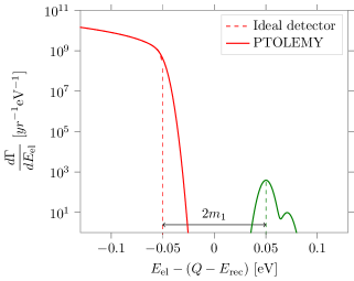
Figure 1: The $\beta$-spectrum of free monoatomic Tritium centered around $Q-E_{\text{rec}}$, where $Q$ is the decay energy and $E_{\text{rec}}$ - recoil of the nucleus in the vacuum. The normal neutrino mass hierarchy Qian and Vogel (2015) is assumed with the mass of the lightest neutrino $m_{1}=$50\text{\,}\mathrm{meV}$$. The spontaneous $\beta$-decay spectrum is shown in red while the C$\nu$B feature is shown in green. The solid lines are drawn assuming a $10\,\rm meV$ resolution of the detector.

The main goal of the C$\nu$B detection experiments is to detect the electrons produced in the neutrino capture channel (see FIG. 1) that depends on the mass of the lightest neutrino and the hierarchy Mertens et al. (2015); Masood et al. (2007); Betti et al. (2019); Baracchini et al. (2018). Since the captured relic neutrinos are soft, it has a shape of $3$ narrow peaks  separated from the end of the main part of the spectrum by double the mass of the lightest neutrino. The spectrum depicted on FIG. 1 is calculated for an isolated Tritium atom in the rest frame, where the recoil energy is defined by the conservation laws. However, if Tritium is absorbed on a substrate, it can not be considered at rest and the recoil energy of the nucleus acquires some amount of uncertainty and so does the measured spectrum of the emitted electron (see FIG. 3).

Two complementary views on such an uncertainty are possible, both leading to the same conclusion in the present context. In the “semiclassical” view the source of the uncertainty is the zero-point motion of the Tritium atom, which results in a fluctuating centre of mass frame at the moment of $\beta$-decay. In the fully quantum view the uncertainty results from quantum transitions of an atom into the highly excited vibrational states in the potential which confines it to the graphene sheet. We shall begin our discussion with the semi-classical picture.

It follows from Heisenberg uncertainty principle that an atom restricted to some finite region in space by the bonding potential cannot be exactly at rest. Even in the zero temperature limit it performs a zero-point motion so that its velocity fluctuates randomly obeying some probability distribution $\mathcal{F}(\mathbf{u}).$ For localized states, $\mathcal{F}(\mathbf{u})$ has a vanishing mean and dispersion defined by the Heisenberg uncertainty principle $\Delta u\sim\hbar/m_{\text{nucl}}\lambda_{\text{nucl}}$. Due to these random fluctuations in the velocity of the nucleus, the observed velocity distribution of the emitted electron in the laboratory frame is given by the convolution

$$\tilde{\mathcal{G}}(\mathbf{v})=\int du\mathcal{F}(\mathbf{u})\mathcal{G}(\mathbf{v}+\mathbf{u}).$$ (2)

where $\mathcal{G}(\mathbf{v})$ is the velocity distribution of an electron emitted by a free Tritium atom at rest corresponding to the energy distribution given by a Fermi Golden Rule (see FIG. 1). The formal applicability condition of Eq. (2) is that the spacing between the energy levels of the ${}^{3}\rm{He}^{+}$ ion emerging from $\beta$-decay be much less than the typical recoil energy $\Delta\varepsilon\ll E_{\text{rec}}.$ This condition is readily satisfied for the recoil energy in vacuum $E_{\text{rec}}=$3.38\text{\,}\mathrm{eV}$.$ We shall revisit this argument when we turn to the fully quantum picture.

In the following analysis we will restrict ourselves to the particular case of the Tritium atoms adsorbed on the graphene following the PTOLEMY proposal. However the obtained results are also valid for more general bonding potentials (see the discussion at the end).

In the zero temperature limit, the function $\mathcal{F}(\mathbf{u})$ appearing in Eq. (2) is encoded in the wave function of the stationary state of a Tritium atom in the potential of the interaction of the atom with graphene. Although such a potential has a rather complicated shape, as can be seen from multiple ab-initio studies Moaied et al. (2014); Henwood and Carey (2007); González-Herrero et al. (2019); Ivanovskaya et al. (2010), the large mass of the nucleus justifies the use of the harmonic approximation near a local potential minimum

$$U=\frac{1}{2}\kappa_{i,j}r_{i}r_{j}+U_{0}$$

where $r_{i}$ are the components of the atom’s displacement vector and $\kappa$ is the Hessian tensor. Then, it follows that $\mathcal{F}(\mathbf{u})$ is a multivariate normal distribution

$$\mathcal{F}(\mathbf{u})=\dfrac{1}{(2\pi)^{3/2}}\dfrac{1}{\sqrt{\det\Sigma}}\exp\left(-\dfrac{1}{2}\sum_{i,j=1}^{3}u_{i}\Sigma^{-1}_{i,j}u_{j}\right).$$ (3)

with zero mean and a covariance matrix $\Sigma=\hbar m^{3/2}\sqrt{\kappa}.$ To find the latter, we proceed to the analysis of the bonding potential near its minima.

An adsorbed Tritium atom is predicted to occupy a symmetric position with respect to the graphene lattice, characterised by a C₃ point symmetry group. For this reason, the Hessian will generally have two distinct principal values, one corresponding to the axis orthogonal to graphene and one to the motion in the graphene plane yielding two different potential profiles.

According to the ab initio studies Ivanovskaya et al. (2010); Henwood and Carey (2007); González-Herrero et al. (2019); Moaied et al. (2014), the potential that bonds the Tritium atom in the perpendicular direction has two minima, a deep chemisorbtion minimum (in the range of $0.7-$3\text{\,}\mathrm{eV}$$ for different studies) about $1.5\rm\ \AA$ away from the graphene plane, and a shallow (about $0.2\text{\,}\mathrm{eV}$) physisorption minimum $3\rm\ \AA$ away from graphene  (see FIG. 2).

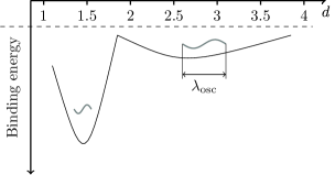
Figure 2: Schematic profile of the potential that bonds the Tritium atom in the direction perpendicular to the graphene.

The lateral motion of an atom is governed by the so-called migration potential Boukhvalov (2010). The lateral stiffness in the case of chemisorption smaller than the vertical stiffness, however is substantial, as can be seen from Table 1. The case of a substrate producing a negligible migration potential will be discussed below.

Introducing the normal displacement $z$ of an atom relative to the potential minimum, we can approximate the potential in the direction perpendicular to the graphene as $U(z)=\kappa z^{2}/2+U_{0}.$ The uncertainty in the position of the nucleus is then characterised by the oscillator length $\lambda^{2}=\hbar/\sqrt{m_{\rm nucl}\kappa}.$ The values of the constants $\kappa$ and $\lambda$ for different potential minima obtained from the fitting of the theoretical bonding profiles Moaied et al. (2014); Henwood and Carey (2007); González-Herrero et al. (2019); Ivanovskaya et al. (2010) are given in Table 1. The pronounced variability in the predicted values of the spring constant $\kappa$ is explained by the diversity of approximations used in different ab initio schemes. Note, however that the variability in the predicted values of the oscillator length is much less significant as $\lambda\sim\kappa^{-\frac{1}{4}}$. For this reason one can crudely neglect the difference between the strength of the lateral and normal confinement and consider the function $\mathcal{F}(\mathbf{u})$ as approximately isotropic

$$\mathcal{F}(\mathbf{u})\approx\dfrac{1}{\sqrt{2\pi}\Delta u}\exp\left(-\dfrac{1}{2}\dfrac{u^{2}}{\Delta u^{2}}\right).$$ (4)

We also note that, according to the Table 1, the typical predicted oscillator length is about an order of magnitude less than the typical length of the bond, which provides a posterior justification for the harmonic approximation.

Potential	Source	$\kappa,\left[$\text{\,}\mathrm{eV}\mathrm{/}\mathrm{\SIUnitSymbolAngstrom}^{2}$\right]$	$\lambda,\left[$\text{\,}\mathrm{\SIUnitSymbolAngstrom}$\right]$	$\Delta E,\left[$\text{\,}\mathrm{eV}$\right]$
	González-Herrero et al. (2019)	2.15	0.16	0.60
Chemisorption	Moaied et al. (2014), GGA	4.62	0.13	0.73
	Moaied et al. (2014), vdW-DF	4.9	0.13	0.75
Physisorption	Ivanovskaya et al. (2010)	0.08	0.37	0.26
	González-Herrero et al. (2019)	0.09	0.34	0.28
	Moaied et al. (2014), GGA	0.18	0.29	0.33
	Moaied et al. (2014), vdW-DF	0.13	0.32	0.3
	Henwood and Carey (2007), GGA	0.04	0.43	0.22
	Henwood and Carey (2007), LDA	0.01	0.55	0.17
Migration	Boukhvalov (2010)	0.283	0.264	0.37

Table 1: Harmonic fit with the stiffness $\kappa$ of the chemisoption, physisorption potentials and the migration potential of the chemisorbed atom profiles near the minimum. $\lambda^{2}=\hbar/\sqrt{m_{\text{nucl}}\kappa}$ and $\Delta E$ is the energy broadening of the emitted electron estimated from Eq. (5).

Estimate —  We are now in a position to obtain an estimate for the uncertainty in the energy of an emitted electron. By virtue of Heisenberg uncertainty principle, the variance of the velocity of the nucleus near a local potential minimum is $\Delta u\approx\hbar/{m_{\text{nucl}}\lambda}.$ For an electron emitted at speed $v_{\text{el}}$ in the centre of mass frame the uncertainty of the energy measured in the laboratory frame is $\Delta E\approx m_{\text{el}}v_{\text{el}}\Delta u,$ which near the edge of the electron emission spectrum can be written as

$$\Delta E\approx\frac{\hbar c}{\lambda_{\rm el}}\gamma$$ (5)

where $\lambda^{2}_{\rm el}\equiv\hbar/\sqrt{m_{\rm el}\kappa}$ and we have introduced the dimensionless parameter

$$\gamma=\left[\frac{Q^{2}m_{\rm el}}{m_{\text{nucl}}^{3}c^{4}}\right]^{1/4},$$ (6)

where $Q$ is the amount of energy released during the $\beta$ decay. Eqns. (5), (6) are the main result of this paper. This result, obtained so far using semi-classical considerations, can be cross-checked with a more precise quantum mechanical calculation. For the latter, one applies the Fermi Golden Rule to the $\beta$-decay process where the initial state is the ground state of the atom in the harmonic potential and the final state is a product of neutrino, electron and atomic wave-functions that are highly excited WKB states (see Appendix A for the detailed calculation). The result of such a calculation fully agrees with Eqns. (5), (6). It is worth noting that in the fully quantum picture the final $\beta$-spectrum in the C$\nu$B channel may be continuous, discrete or mixed, depending on the depth of the bonding potential, but the overall envelope will be Gaussian with the width $\Delta E$. This is in agreement with the previous results for the molecular Tritium Bodine et al. (2015) .

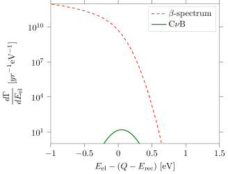
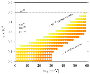
Figure 3: The estimate of the smearing of the electron emission spectrum due to the bonding of emitter to graphene. Left panel: The electron emission spectrum for the physisorbed atomic Tritium ($\lambda_{\text{osc}}=$0.6\text{\,}\mathrm{\SIUnitSymbolAngstrom}$$) taking the hierarchy, $m_{1}$ and energy resolution of the apparatus same as for the FIG. 1. Right panel: Visibility(defined by the number of C$\nu$B event that do not overlap with the continuous spectrum at all) of the C$\nu$B peak depending on the mass of the lightest neutrino $m_{1}$ and a dimensionless parameter $\gamma$ defined in Eq. (6) that characterizes the emitter (for the physisorbed Tritium $\gamma\approx 3\times 10^{-4}$). The white areas on the bottom right and top left are correspondingly the areas of full and zero visibility and the coloured region in between corresponds to the partial visibility.

Discussion —  In this paper, we have investigated the feasibility of the solid state based approach to the long-standing problem of detection of relic neutrino background. We conclude that, due to the remarkable progress in the technology used for the measurement of electron emission spectrum (see e.g.  Baracchini et al. (2018)) , the actual energy resolution of the experiment is now controlled by a different bottleneck - the uncertainties resulting from the interaction of the beta-emitter with the substrate. This paper addresses one type of such uncertainty considered – the zero-point motion of the $\beta$-emitter. For any given emitter it is practically irreducible, which excludes certain emitters from the list of suitable candidates for solid state setups. In particular, for Tritium the uncertainty in the energy of the electrons is around $0.3-$0.7\text{\,}\mathrm{eV}$$ (see Table 1 for the different bonding potentials according to different ab initio calculations), i.e. several times greater than the required energy resolution.

We see from Eqns. (5), (6) that the defining factor for the energy uncertainty is the parameter $\gamma$ (see Eq. 6), which only depends on the internal properties of a $\beta$-emitter such as the mass of the nucleus and the energy released in the decay process. Therefore, a promising route to achieve a better performance of the detector would be to substitute a widely used Tritium Baracchini et al. (2018); Faessler et al. (2013); Wolf et al. (2010); Cocco (2017); Betts et al. (2013); Betti et al. (2019) with a heavier emitter (while simultaneously satisfying other experimental constraints, e.g. sufficiently long half-life time). The effect of the parameter $\gamma$ on the visibility of the C$\nu$B peak is shown on the right panel of FIG. 3. One can see that, e.g., Tritium which has $\gamma\approx 3\times 10^{4},$ lies deep inside the region where the observation of the C$\nu$B peak is impossible. On the same figure we also indicate more suitable $\beta$-emitters whose energy uncertainties are not prohibitive for the detection of the relic neutrinos with the masses $>$20\text{\,}\mathrm{meV}$$.

Another important conclusion of our work is that although the energy uncertainty also depends on the bonding potential, this dependence only enters through the stiffness parameters and it is extremely weak $\Delta E\propto\kappa^{1/4}$. This implies that experimentation with different types of substrate is unlikely to make a substantial difference. Indeed, an order of magnitude improvement in $\Delta E,$ (which is needed for the state of the art experimental proposal Baracchini et al. (2018)) would require a four orders of magnitude reduction in the value of $\kappa.$ Such a substantial deformation of the bonding potential presents a significant experimental challenge.

A certain improvement in terms of the bonding potential could still be achieved with adsorption that has a very weak lateral potential. One such example is physisorption of Tritium on graphene. In the limiting case of a constant lateral potential, electrons emitted at grazing angles will not have any additional uncertainty to their energy. Correspondingly, for the out-of-plane angles $\theta<\theta_{\text{max}}=\arcsin\left(\Delta E_{\text{max}}/\Delta E\right)$ the energy uncertainty will be bounded by $\Delta E_{\text{max}}$. Here $\Delta E$ denotes the energy uncertainty for the isotropic case with finite mobility. Restricting the detection collection to $\theta<\theta_{\text{max}}$ reduces the number of events by a factor $\eta^{-1}\approx\pi\theta_{\text{max}}/90^{\circ}$. As an example, for $\Delta E_{\text{max}}=$10\text{\,}\mathrm{meV}$$ one obtains $\theta_{\text{max}}\approx 3^{\circ},\eta\approx 10$ which would entail the challenge of producing and handling 10 times as much radioactive material. This direction requires a full in-depth analysis which we leave for future studies.

We conclude, that a careful selection of the $\beta$-emitter (Fig. 3) together with the use of an optimized substrate place C$\nu$B detection potentially within the reach of the detection technologies developed by the PTOLEMY collaboration.

One should, however, note that the zero-point motion of the emitter does not exhaust the list of mechanisms that introduce uncertainty and errors into the beta-decay spectrum. Other potentially harmful mechanisms include the electrostatic interaction of the ionized atom with the substrate, charge relaxation in graphene, $X$-ray edge singularity, and phonon emission. We therefore strongly believe that further progress towards C$\nu$B detection requires a serious concerted effort both theoretical and experimental in the characterization of the physics and chemistry of the interaction of the $\beta$-emitter with its solid state environment.

Acknowledgements — We are grateful to Chris Tully, A.P. Colijn and the whole PTOLEMY collaboration for fruitful discussions and feedback on the manuscript that allowed for its significant improvement. We also thank Kyrylo Bondarenko and Anastasiia Sokolenko for the useful discussion. YC is supported by the funding from the Netherlands Organization for Scientific Research (NWO/OCW) and from the European Research Council (ERC) under the European Union’s Horizon 2020 research and innovation programme. AB is supported by the European Research Council (ERC) Advanced Grant “NuBSM” (694896). VC is grateful to the Dutch Research Council (NWO) for partial support, grant No 680-91-130.

Appendix A Quantum derivation of the energy uncertainty

The aim of the fully quantum derivation is to underpin the semiclassical heuristic that was obtained in the main text as well as demonstrating its limitations. We note that we will not keep track of the pre-factors $\hbar,c$ and will restore them in the end. The rate of $\beta$-emission of an electron is given by the Fermi Golden Rule rule

$$\frac{d\Gamma}{dE}=\sum_{f}2\pi|\braket{f}{\hat{V}}{i}|^{2}\delta(E_{i}-E_{f})\delta(E-E_{f,\rm el}).$$ (7)

Here the vector $|i\rangle$ represents the initial state of the system having the energy $E_{\rm i},$ the vector $|f\rangle,$ represents a final eigenstate of the Hamiltonian having the energy $E_{f}=E_{f,\rm el}+E_{f,\rm He}$ where $E_{f,\rm el},$ is the kinetic energy of the outgoing electron and $E_{f,\rm He},$ is the energy of the ${}^{3}\rm He^{+}$ ion. The sum is performed over all such final states. The interaction potential $\hat{V}$ is responsible for $\beta$-decay vertex and is for our purposes an ultralocal product of the creation and annihilation operators of the fields involved in the process.

We make an assumption that the neutrino has zero kinetic energy. It is equivalent to restricting ourselves to region near the edge of the spectrum, which is exactly the region of interest to us. The energy conservation implies

$$\dfrac{\vec{k}^{2}}{2m_{\text{el}}}+\dfrac{\vec{p}^{2}}{2m_{\text{nucl}}}=\tilde{Q},$$ (8)

where $\vec{k}$, $\vec{p}$ - are two-dimensional final momenta of the electron and nucleus respectively. $\tilde{Q}$ is the total energy of the nucleus before $\beta$-decay.

The initial state of the system is a product of a plane wave state of an incoming relic neutrino, which it is safe to describe as a plane wave with nearly zero momentum, and the lowest energy eigenstate of a Tritium atom in the local minimum of the bonding potential. As was discussed in the main text, such a state can be safely approximated as a ground state of a harmonic oscillator with two distinct principal stiffness eigenvalues (see table 1). The wave funcion of such a state has the form

$$\psi_{\text{i}}(\mathbf{r})\propto\exp\left(-\dfrac{z^{2}}{2\lambda_{\perp}^{2}}-\dfrac{\varrho^{2}}{2\lambda_{\parallel}^{2}}\right),$$ (9)

where $z$ stands for the orthogonal displacement and $\varrho$ for the magnitude of the lateral displacement relative to the local potential minimum. Due to the in-plane symmetry of the graphene with respect to rotation, we can effectively restrict ourselves to a two-dimensional space $z,\varrho$.

The space of all possible final states $\ket{f}$ is quite large, and their wave functions may be quite complicated due to the intricate interaction of the ${}^{3}\rm He^{+}$ ion with the graphene sheet. However, as we shall see momentarily the dominant contribution to the sum in (7) comes from the states which are amenable to the WKB approximation and are therefore analytically tractable. Introducing the notation $\psi_{f}(\mathbf{r})$ for the final state of the ${}^{3}\rm He^{+}$ ion, we write the matrix element in (7) as

$$\bra{f}\hat{V}\ket{i}\sim\int d\mathbf{r}\psi^{*}_{f}(\mathbf{r})\psi_{i}(\mathbf{r})e^{-i\mathbf{k}\mathbf{r}}$$ (10)

where $\mathbf{k}$ is the wave vector of the emitted electron at kinetic energy close to $Q.$ Since the electron’s wave vector is quite large $k\sim 10^{2}\,{\AA}^{-1}$ the rapid oscillations suppress the integral in Eq. (10) unless the state $\psi_{f}(\mathbf{r})$ also contains an oscillatory factor, which has a roughly opposite De Broglie wave vector near $\mathbf{r}=0,$ where the support of $\psi_{i}(\mathbf{r})$ is concentrated. This implies that the kinetic energy of the ion needs to be on the order of $3$eV, which exceeds the predicted chemisorption binding energy Ivanovskaya et al. (2010); Henwood and Carey (2007); González-Herrero et al. (2019); Moaied et al. (2014) and is orders of magnitude greater than the vibrational quantum near the potential minimum ($\hbar\omega\sim 0.01$ eV). Such highly excited states are generally characterised by a level spacing which is much narrower than the vibrational quantum near the minimum. They are also well described by semiclassical WKB wave functions, which on the scale of the oscillator length are indistinguishable from a plane wave.

With these considerations in mind, the application of the Fermi Golden Rule to such states gives

$$\dfrac{d\Gamma}{dE}\propto\left|\int_{-\infty}^{\infty}dx\int_{-\infty}^{\infty}dy\int_{-\infty}^{\infty}dz\exp\left(-i(k_{x}+p_{x})x-i(k_{y}+p_{y})y-i(k_{z}+p_{z})z-\dfrac{x^{2}}{2\lambda^{2}_{\parallel}}-\dfrac{y^{2}}{2\lambda^{2}_{\parallel}}-\dfrac{z^{2}}{2\lambda^{2}_{\perp}}\right)\right|^{2},$$ (11)

where we have extended the integration over $z$ to $-\infty$. One can do it since the integrand is localized. $k/p_{x,y,z},$ are respectively the components of the electron and nucleus momenta that satisfy the energy conservation law

$$|p| =\sqrt{2m_{\text{nucl}}\left(\tilde{Q}-E_{\text{el}}\right)}$$

$$|k| =\sqrt{2m_{\text{el}}E_{\text{el}}}$$ (12)

We re-scale coordinates $\tilde{r}_{i}=\dfrac{r_{i}}{\sqrt{2}\lambda_{i}}$ and obtain

$$\dfrac{d\Gamma}{dE}\propto\left|\int_{-\infty}^{\infty}d\tilde{x}\int_{-\infty}^{\infty}d\tilde{y}\int_{-\infty}^{\infty}d\tilde{z}\exp\left(-i\sqrt{2}\lambda_{\parallel}(k_{x}+p_{x})-i\sqrt{2}\lambda_{\parallel}(k_{y}+p_{y})-i\sqrt{2}\lambda_{\perp}(k_{\perp}+p_{\perp})\tilde{z}-\tilde{x}^{2}-\tilde{y}^{2}-\tilde{z}^{2}\right)\right|^{2},$$ (13)

that can be brought to a Gauss integral

$$\dfrac{d\Gamma}{dE} \propto e^{-\lambda^{2}_{\perp}(k_{\perp}+p_{\perp})^{2}-\lambda^{2}_{\parallel}(k_{\parallel}+p_{\parallel})^{2}}\times$$

$$\left|\int_{-\infty}^{\infty}d\tilde{x}\int_{-\infty}^{\infty}d\tilde{y}\int_{-\infty}^{\infty}d\tilde{z}\exp\left(-\left(\tilde{x}+\dfrac{i\lambda_{\parallel}(k_{x}+p_{x})}{\sqrt{2}}\right)^{2}-\left(\tilde{y}+\dfrac{i\lambda_{\parallel}(k_{y}+p_{y})}{\sqrt{2}}\right)^{2}-\left(\tilde{z}+\dfrac{i\lambda_{\perp}(k_{z}+p_{z})}{\sqrt{2}}\right)^{2}\right)\right|^{2},$$ (14)

where $k_{\parallel}/p_{\parallel}^{2}=k_{x}/p_{x}^{2}+k_{y}/p_{y}^{2},p_{\perp}/p_{\perp}=k_{z}/p_{z}$. Integrating Eq. A gives the Gaussian distribution

$$\dfrac{d\Gamma}{dE}\propto e^{-\lambda^{2}_{\perp}(k_{\perp}+p_{\perp})^{2}-\lambda^{2}_{\parallel}(k_{\parallel}+p_{\parallel})^{2}}.$$ (15)

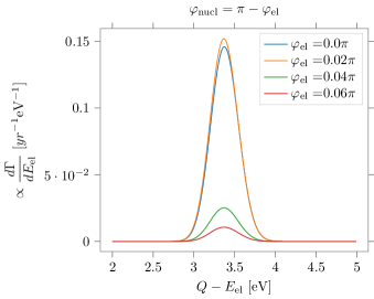
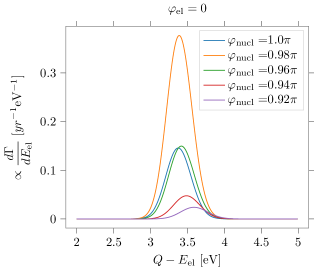
Figure 4: Distribution function (not normalized) of the energy of the electron near the edge of the spectrum. Electron and nucleus are emitted with the corresponding angles $\varphi_{e/\text{nucl}}$ (relative to the axes perpendicular to the graphene substrate).

The distribution Eq. (15) depends on the angles of the emitted nucleus and electron $\varphi_{1,2}$. These angles are taken relative to the axes perpendicular to the graphene substrate.

$$\dfrac{d\Gamma}{dE}\propto e^{-\lambda^{2}_{\perp}\left(|k|\cos\varphi_{2}+|p|\cos\varphi_{1}\right)^{2}-\lambda^{2}_{\parallel}\left(|k|\sin\varphi_{2}+|p|\sin\varphi_{1}\right)^{2}},$$ (16)

Let us estimate the variance of this distribution for the normal emission of the electron

$$\dfrac{d\Gamma}{dE}\propto e^{-\lambda^{2}\left(k-p\right)^{2}},$$ (17)

where $k=\sqrt{2m_{\text{el}}E_{\text{el}}},p=\sqrt{2m_{\text{nucl}}\left(\tilde{Q}-E_{\text{el}}\right)}$.

In order to obtain the variance, wee need to expand near the maximum of the distribution that corresponds to its mean. If we write everything in terms of the deviation from the mean energy of the electron $\delta E_{\text{el}}=\tilde{Q}-E_{\text{rec}}-E_{\text{el}}$

$$k =\sqrt{2m_{\text{el}}\left(\tilde{Q}-E_{\text{rec}}-\delta E_{\text{el}}\right)}\approx\sqrt{2m_{\text{el}}\left(\tilde{Q}-E_{\text{rec}}\right)}\left(1-\dfrac{\delta E_{\text{el}}}{2(\tilde{Q}-E_{\text{rec}})}\right)$$

$$p =\sqrt{2m_{\text{nucl}}\left(E_{\text{rec}}+\delta E_{\text{el}}\right)}\approx\sqrt{2m_{\text{nucl}}E_{\text{rec}}}\left(1+\dfrac{\delta E_{\text{el}}}{2E_{\text{rec}}}\right).$$ (18)

Accounting to the fact that $E_{\text{rec}}\approx\dfrac{m_{\text{el}}}{m_{\text{nucl}}}\tilde{Q}$,

$$k \approx\sqrt{2m_{\text{el}}\tilde{Q}}\left(1-\dfrac{\delta E_{\text{el}}}{2\tilde{Q}}\right)$$

$$p \approx\sqrt{2m_{\text{el}}\tilde{Q}}\left(1+\dfrac{m_{\text{nucl}}}{m_{\text{el}}}\dfrac{\delta E_{\text{el}}}{2\tilde{Q}}\right).$$ (19)

With this we obtain Gaussian distribution

$$\dfrac{d\Gamma}{dE}\propto\exp \left(-\dfrac{\lambda^{2}m_{\text{nucl}}^{2}}{2m_{\text{el}}\tilde{Q}}\delta E_{\text{el}}^{2}\right),$$

with the variance with the restored units is

$$\sigma=\dfrac{\hbar}{\lambda}\dfrac{\sqrt{\tilde{Q}m_{\text{el}}}}{m_{\text{nucl}}}.$$ (20)

References

- Weinberg (1962) S. Weinberg, Physical Review 128, 1457 (1962).
- Baracchini et al. (2018) E. Baracchini, M. Betti, M. Biasotti, A. Bosca, F. Calle, J. Carabe-Lopez, G. Cavoto, C. Chang, A. Cocco, A. Colijn, et al., arXiv preprint arXiv:1808.01892 (2018).
- Follin et al. (2015) B. Follin, L. Knox, M. Millea, and Z. Pan, Physical review letters 115, 091301 (2015).
- Cocco et al. (2007) A. G. Cocco, G. Mangano, and M. Messina, JCAP 06, 015 (2007), arXiv:hep-ph/0703075 .
- Faessler et al. (2017) A. Faessler, R. Hodák, S. Kovalenko, and F. Šimkovic, in Quarks, Nuclei and Stars: Memorial Volume Dedicated to Gerald E. Brown (World Scientific, 2017) pp. 81–91.
- Cocco et al. (2009) A. G. Cocco, G. Mangano, and M. Messina, Physical Review D 79, 053009 (2009).
- Betti et al. (2019) M. Betti et al. (PTOLEMY), JCAP 07, 047 (2019), arXiv:1902.05508 [astro-ph.CO] .
- Note (1) The capture spectrum comprises of three peaks corresponding to the three neutrino mass eigenstates. The first two peaks overlap and are barely distinguishable.
- Wolf et al. (2010) J. Wolf, K. Collaboration, et al., Nuclear Instruments and Methods in Physics Research Section A: Accelerators, Spectrometers, Detectors and Associated Equipment 623, 442 (2010).
- Bodine et al. (2015) L. Bodine, D. Parno, and R. Robertson, Physical Review C 91, 035505 (2015).
- Note (2) In general, the interaction of an adsorbed radioactive atom with the substrate is complicated and it gives rise to several effects each contributing to the broadening of the measured -emission spectrum. In this paper, we only focus on one which is arguably the simplest and the strongest of all: the zero-point motion of an atom arising from the atom’s adsorption.
- Betts et al. (2013) S. Betts, W. Blanchard, R. Carnevale, C. Chang, C. Chen, S. Chidzik, L. Ciebiera, P. Cloessner, A. Cocco, A. Cohen, et al., arXiv preprint arXiv:1307.4738 (2013).
- Messina (2018) M. Messina, Frascati Phys. Ser. (2018).
- Cocco (2017) A. G. Cocco, PoS (2017), 10.22323/1.283.0092.
- Li (2015) Y.-F. Li, International Journal of Modern Physics A 30, 1530031 (2015).
- Long et al. (2014) A. J. Long, C. Lunardini, and E. Sabancilar, Journal of Cosmology and Astroparticle Physics 2014, 038 (2014).
- Qian and Vogel (2015) X. Qian and P. Vogel, Progress in Particle and Nuclear Physics 83, 1 (2015).
- Mertens et al. (2015) S. Mertens, T. Lasserre, S. Groh, G. Drexlin, F. Glueck, A. Huber, A. Poon, M. Steidl, N. Steinbrink, and C. Weinheimer, Journal of Cosmology and Astroparticle Physics 2015, 020 (2015).
- Masood et al. (2007) S. S. Masood, S. Nasri, J. Schechter, M. A. Tórtola, J. W. Valle, and C. Weinheimer, Physical Review C 76, 045501 (2007).
- Note (3) Each of the peak corresponds to a separate mass eigenstate.
- Moaied et al. (2014) M. Moaied, J. Moreno, M. Caturla, F. Ynduráin, and J. Palacios, arXiv preprint arXiv:1405.3165 (2014).
- Henwood and Carey (2007) D. Henwood and J. D. Carey, Physical Review B 75, 245413 (2007).