Localization in the Kicked Ising Chain

Abstract

Determining the border between ergodic and localized behavior is of central interest for interacting many-body systems. We consider here the recently very popular spin-chain model that is periodically excited. A convenient description of such a many-body system is achieved by the dual operator that evolves the system in contrast to the time-evolution operator not in time but in particle direction. We identify in this paper the largest eigenvalue of a function based on the dual operator as a convenient tool to determine if the system shows ergodic or many-body localized features. By perturbation theory in the vicinity of the noninteracting system we explain analytically the eigenvalue structure and compare it with numerics in [P. Braun, D. Waltner, M. Akila, B. Gutkin, T. Guhr, Phys. Rev. E 101, 052201 (2020)] for small times. Furthermore we identify a quantity that allows based on extensive large-time numerical computations of the spectral form factor to distinguish between localized and ergodic system features and to determine the Thouless time, i.e. the transition time between these regimes in the thermodynamic limit.

I Introduction

Interacting spin systems play a prominent role in the study of many-body quantum systems, in particular, of many-body quantum chaos. Prominent examples are the Ising model Bogomolny ; Keating ; Heidel ; Moessner0 ; Papic , the Heisenberg model Znidaric ; Langer ; Gemmer but also other models like the Bose-Hubbard model Urbina ; Dubertrand and coupled kicked tops And are considered. In the experimentally most relevant case of spin $1/2$ semiclassical methods successful in the theory of the few-body chaos Fritz ; Stockmann are inapplicable and alternative approaches are needed. A very popular one applicable to a large class of kicked chains is the method of the dual operator in which the evolution time $t$ and the particle number $N$ exchange their roles Akila ; it is especially suited to study the thermodynamic limit when $N$ is very large. Statistical properties of the spectra are then expressed in terms of the “dual operator” replacing the Floquet operator of the standard approach.

In the last years this dual perspective became extremely popular to describe spectral properties Prosen ; Chalker ; ChalkerI ; Braun ; Flak , to quantify entanglement ProsenII ; Pal ; Lamacraft , correlation functions Gutkin ; ProsenIII ; LamacraftI and the connection between quantum and classical system properties AkilaI ; ChalkerII . The dual operator is usually non-unitary, however in the case of the so called self-duality or self-unitarity, it is. A remarkable property of strongly disordered self-dual chains is that they allow on the one hand for an analytically exact description of many system properties and on the other hand they are completely chaotic, two features usually considered as contradictory. This applies to the spectral form factor Prosen ; Chalker ; ChalkerI ; Braun ; Flak determining the correlations between discrete quantum levels that behaves in accordance with Random Matrix Theory (RMT) Meta ; Guhr already for short times as long as the number of constituents $N$ of the chain is large, to the entanglement entropy ProsenII ; Pal ; Lamacraft and correlation functions Gutkin ; ProsenIII ; LamacraftI . The RMT behavior of the disordered kicked Ising chain (KIC) and ergodicity Prosen0 with parameters corresponding to self-duality have been proven in Prosen . The method was based on analytic averaging of the form factor in the dual representation.

Whereas Ref. Prosen concentrated on the self-dual parameter regime, in Ref. Braun we studied the spectral form factor of the strongly disordered KIC in the regime where the self-duality condition is violated by changing the Ising interaction constant. When that constant is brought to zero the resulting chain of independent spins is trivially localized such that somewhere on the way a transition between the ergodic and localized phase is bound to take place. First indications of that transition were given in Braun . However, the drawback was here that the standard $N$ resolved quantities to detect a transition to many-body localization like the spacing ratio or the entanglement entropy considered can only be obtained for small $N$, see e.g. Ref. Papic . An analogous statement applies to the largest eigenvalue of the double dual operator that is a function of the dual operator: it can be computed only for a small number of timesteps Braun . The aim of this paper is to solve this problem: by extensive numerical calculations of the spectral form factor we are able to compute this eigenvalue also for much larger times. This is especially relevant as localization is a system feature that can only be probed in the limit of large (optimally infinite) times and system sizes. Independently, as the dual-operator method became during the last years an extremely popular method to analyse various system features Akila ; Prosen ; Chalker ; ChalkerI ; Braun ; Flak ; ProsenII ; Pal ; Lamacraft ; Gutkin ; ProsenIII ; LamacraftI ; AkilaI ; ChalkerII ; Prosenarx the understanding of the eigenvalue structure of this operator is also a topical research question on its own.

The outline of the paper is as follows: In the next section we introduce the relevant quantities and recapitulate previous results. In Section III we develop a perturbation theory starting from the case of noninteracting spins. Together with our analysis in the vicinity of self duality in Ref. Braun we thus exploit all possible analytical descriptions in the regime where the self-duality condition is violated. In Section IV we briefly recapitulate our numerical calculations in Ref. Braun for the eigenvalue of the double dual operator of largest magnitude with times $t$ up to $20$. In Section V we present a method to determine that eigenvalue from the numerical form factor for times much larger than in the previous section but smaller than the Heisenberg time $T_{H}$; we demonstrate its characteristic change in the crossover between the ergodic and localized regime. These results allow to determine the Thouless time as described in Section VI. We conclude in Section VII and present technical details in the Appendix.

II Basic Evolution Operators and the Spectral Form Factor

We consider the disordered KIC with ring topology consisting of $N$ spins $1/2$. The evolution operator of the system per period, i. e. the Floquet operator, reads,

$$\hat{U} =\hat{U}_{I}\hat{U}_{b},$$ (1)

$$\hat{U}_{I} =\exp\left(-iJ\sum_{n=1}^{N}\hat{\sigma}_{n}^{z}\hat{\sigma}_{n+1}^{z}\right),$$

$$\hat{U}_{b} =\exp\left(-i\sum_{n=1}^{N}h_{n}\hat{\sigma}_{n}^{z}\right)\exp\left(-ib_{x}\sum_{n=1}^{N}\hat{\sigma}_{n}^{x}\right).$$

The factor $\hat{U}_{I}$ describes the Ising interaction between the neighboring spins with the interaction constant $J$. The second factor in the operator $\hat{U}_{b}$ can be interpreted as a kick by the magnetic field $b_{x}$ in the transverse direction while the first one characterizes longitudinal local magnetic fields randomly distributed along the chain. The operator $\hat{U}$ acts in the Hilbert space with the dimension $2^{N}$ spanned by the basis vectors $\left|\sigma_{1},\ldots,\sigma_{N}\right\rangle$ with $\sigma_{n}=\pm 1$. We consider here as in Ref. Braun the orthogonal kick strength fixed, $b_{x}=\pi/4$ and the Ising constant changing from $J=\pi/4$ to $0$.

The spectral form factor is defined by,

$$K_{N}\left(t\right)=\left\langle\left|\operatorname*{Tr}\hat{U}^{t}\right|^{2}\right\rangle/T_{H},$$ (2)

where $T_{H}=2^{N}$ is the Heisenberg time for the chain of spins $1/2$; averaging is over the disorder realizations. If the disorder on different spins is uncorrelated averaging can be performed analytically provided the disorder statistics is given. Assuming the local fields $h_{n}$ to be Gaussian-distributed it was shown in Refs. Prosen ; Braun that

$$K_{N}\left(t\right)=\operatorname*{Tr}\left(\mathcal{A}_{\xi}\left(t\right)\right)^{N}/T_{H}.$$

The time-dependent operator $\mathcal{A}_{\xi}(t)$ acts in the ”squared” dual Hilbert space with the basis $\left|\boldsymbol{\sigma\sigma}^{\prime}\right\rangle=\left|\boldsymbol{\sigma}^{t}\right\rangle\otimes\left|\boldsymbol{\sigma}^{\prime t}\right\rangle$ and dimension $2^{2t}.$ It is given by the Kronecker product

$$\mathcal{A}_{\xi}(t)=\left(\overline{\hat{w}\left(t\right)}\otimes\overline{\hat{w}^{\ast}\left(t\right)}\right)\mathcal{O}_{\xi},$$

where $\overline{\hat{w}(t)}$ is obtained from the factors of the dual operator $\hat{W}_{n}$ defined in Ref. Braun by replacing $h_{n}$ by its disorder-averaged value $h=\left\langle h_{n}\right\rangle$; the operator $\mathcal{O}_{\xi}$ depends on the disorder strength $\xi$. In the limit of large $\xi$ the operator $\mathcal{A}_{\xi}(t)$ turns to the double dual operator

$$\mathcal{A}(t)=\mathcal{P}\left(\overline{\hat{w}\left(t\right)}\otimes\overline{\hat{w}^{\ast}\left(t\right)}\right)\mathcal{P}.$$ (3)

The operator $\mathcal{P}$ is a projector diagonal in the squared dual space with the non-zero elements

$$\left\langle\boldsymbol{\sigma\sigma}^{\prime}\left|\mathcal{P}\right|\boldsymbol{\sigma\sigma}^{\prime}\right\rangle=\left\{\begin{array}[c]{c}1,\quad\sum_{k=1}^{t}\sigma_{k}=\sum_{k=1}^{t}\sigma_{k}^{\prime},\\ 0,\quad\text{otherwise.}\end{array}\right.$$

Since $K_{N}\left(t\right)=\sum_{s}\lambda_{s}^{N}\left(t\right)/2^{N}$ where $\lambda_{s}(t)$ are the eigenvalues of $\mathcal{A}(t)$, we found in Ref. Braun that only the contribution of the largest $\lambda_{s}(t)$ by magnitude denoted by $\lambda_{0}(t)$ is of importance that turns out to be real and positive survives when $N\rightarrow\infty$. As proved in Prosen in the self-dual case $\mathcal{A}(t)$ has $2t$ eigenvalues equal to one footn , all other eigenvalues having $\left|\lambda_{s}\right|<1$. Therefore the form factor in the thermodynamic limit tends to $2t/T_{H}$ which is the result obtained by the Gaussian Orthogonal Ensembe (GOE) of RMT in the limit of times much smaller than the Heisenberg time.

For $t$ prime and $\Delta J\equiv\pi/4-J$ small we obtained for the largest eigenvalue of the double dual operator denoted by $\lambda_{0}(t)$ within perturbation theory Braun

$$\lambda_{0}\left(t\right)=1+\Delta J^{2}\frac{2t\left(t-1\right)}{2^{\left(t-1\right)/2}+1}+O\left(\Delta J^{4}\right);$$ (4)

all other eigenvalues of the multiplets shift from one downwards thus forming a gap between $\lambda_{0}\left(t\right)$ and the other levels for nonzero $\Delta J$. The relation (4) with $\Delta J$ fixed and time growing implies that the gap diminishes proportional to $2^{-t/2}$ with the ergodic form factor restored.

III Perturbation theory starting from non-interacting spins

In the other extreme of non-interacting spins, $J=0$ resp. $\Delta J=\pi/4$ when the evolution operator is a product of rotations of individual spins,

$$\hat{U} =\prod_{n=1}^{N}\hat{u}_{n},$$

$$\hat{u}_{n}=\exp\left(ih_{n}\hat{\sigma}_{n}^{z}\right)\exp\left(i\frac{\pi}{4}\hat{\sigma}_{n}^{x}\right)=\exp\left(i\gamma(h_{n})\mathbf{e}_{n}\boldsymbol{\sigma}_{n}/2\right).$$

The rotation around the $x-$direction by $\pi/2$ followed by the random rotation by $2h_{n}$ about $z$ can be replaced by a single rotation about some axis $\mathbf{e}_{n}$ by the angle $\gamma_{n}=\gamma\left(h_{n}\right)$ connected with $h_{n}$ by $1+2\cos 2\gamma_{n}=\cos 2h_{n}$ or

$$\gamma(h)=\arccos\frac{\cos 2h-1}{2}.$$ (5)

Averaging over disorder can be performed independently for each spin, and we get, for all $N$,

$$K_{N}\left(t\right)=\left\langle\frac{1}{2}\left|\operatorname*{Tr}\hat{u}^{t}\right|^{2}\right\rangle^{N},$$

where $\hat{u}$ is obtained from $\hat{u}_{n}$ by replacing $h_{n}$ by its disorder averaged value $h=\langle h_{n}\rangle$. Remembering $K_{N}\left(t\right)=\sum_{s}\lambda_{s}^{N}\left(t\right)/2^{N}$ we see that only one eigenvalue $\lambda_{0}\left(t\right)$ of the operator $\mathcal{A}(t)$ is non-zero and equal to,

$$\lambda_{0}\left(t\right)=\left\langle\left|\operatorname*{Tr}\hat{u}^{t}\right|^{2}\right\rangle,$$

i. e., the operator is proportional to a projector on a single vector in the squared dual Hilbert space. This vector has highest possible symmetry; it is invariant under permutation and reflection of the individual spins as we show in appendix A. In the regime of small $\Delta J$ we found in Ref. Braun that the dominant eigenvalue for small $t$ possessed the same symmetry.

It is easy to calculate $\lambda_{0}\left(t\right)$ in the case of strong disorder assuming all angles of the $z-$rotation $2h_{n}$ to be uniformly distributed in $[0,2\pi]$; then we obtain,

$$\lambda_{0}\left(t\right) =\frac{4}{2\pi}\int_{0}^{2\pi}\cos^{2}t\gamma\left(h\right)dh$$ (6)

$$=2+\left(-1\right)^{k}\frac{\left(2m-1\right)!!}{\left(2m\right)!!},\quad k=\left[\frac{t+1}{2}\right],\quad m=\left[\frac{t}{2}\right].$$

In the limit of large times the stationary phase approximation taking into account the stationary points $h=0$ and $h=\pi$ gives,

$$\lambda_{0}\left(t\right)=2+\left(-1\right)^{k}\sqrt{\frac{2}{\pi t}}.$$ (7)

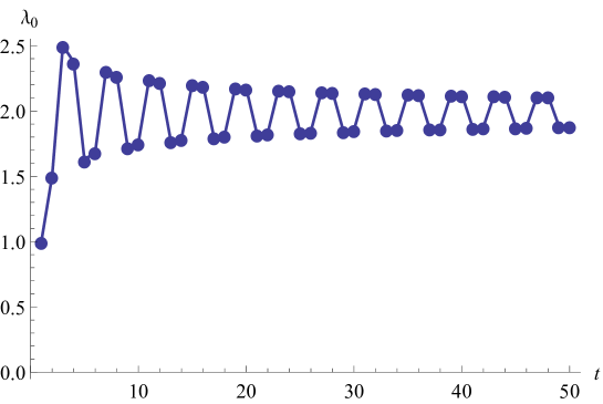
Figure 1: Senior eigenvalue of $\mathcal{A}(t)$ against time, non-interacting spins

Approximate periodicity of $\lambda_{0}\left(t\right)$ with period $\Delta T=4$ is associated with the $x-$rotation angle $\pi/2$; that can be interpreted as the result of interference of the saddle-point contributions to the integral (6). The oscillation with period four die out $\sim t^{-1/2}$ with the growth of time and are suppressed if we average $\lambda_{0}(t)$ over four consecutive times; in both cases we get $\lambda_{0}=2$ and $K_{N}\left(t\right)=1$ which corresponds to the Poissonian RMT statistics.

Perturbation theory can be used to get the eigenvalue $\lambda_{0}\left(t\right)$ for $J$ non-zero but small. The deflection from the limit (6) is quadratic in $J$; the method and the details of the calculation are described in appendix B. Similar to the previous case, the radius of convergence shrinks with the growth of time. Here we get

$$\lambda\left(t\right) = \lambda_{0}\left(t\right)+\frac{tJ^{2}}{\lambda_{0}\left(t\right)}\left[t\left(2-\sum_{k=0}^{[t/2]}\left(\begin{array}[]{c}1/2\\ k\end{array}\right)\right)^{2}-\lambda_{0}^{2}(t)\right.$$ (13)

$$\left.-\sum_{\tau=1}^{t-1}\left(2\left(1-S(\tau-1)+S(t)-S(t-\tau-1)\right)-\left(\begin{array}[]{c}-1/2\\ {[t/2]}\end{array}\right)\right)^{2}\right]$$

with

$$S(\tau)=\sum_{k=0}^{[\tau/2]}\left(\begin{array}[]{c}-1/2\\ k\end{array}\right).$$ (14)

In the left panel of Fig. 2 we compare this perturbative result with the the exact one from numerical calculations. We confirm by this analytically the structure that $\lambda_{0}(t)$ for small nonzero $J$ oscillates around $\lambda_{0}(t)$ for $J=0$ found numerically in Ref. Braun .

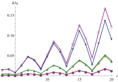
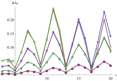
Figure 2: Difference $\Delta\lambda_{0}(J)=\lambda_{0}(J)-\lambda_{0}(0)$ as a function of $t$. Left panel: Perturbation theory up to second order, different curve pairs for $\Delta J=0.8,\,0.76,\,0.74$ from bottom to top, for each $\Delta J$ the lower of the nearby curve obtained numerically the upper one from perturbation theory. Right panel: Perturbation theory up to fourth order, different curve pairs for $\Delta J=0.76,\,0.74,\,0.72,\,0.7$, upper of nearby curve obtained numerically, the lower one from perturbation theory.

Considering the average of $\lambda_{0}(t)$ over the oscillations of period four

$$\langle\lambda_{0}(t)\rangle=\frac{1}{4}\left[\lambda_{0}(t+3)+\lambda_{0}(t+2)+\lambda_{0}(t+1)+\lambda_{0}(t)\right]$$ (15)

we get as shown in appendix B in the limit of large time up to quadratic order in $J$

$$\langle\lambda_{0}(t)\rangle = \lambda_{0}(t)+\frac{tJ^{2}}{\lambda_{0}(t)}\left[-\frac{4(\sqrt{2}-1)}{\sqrt{\pi}}\left[(2-\sqrt{2})\zeta[1/2]-\zeta[1/2,1/4]+\zeta[1/2,3/4]\right]\right.$$ (16)

$$\left.+(2-\sqrt{2})^{2}-4-\frac{4}{\pi}(\gamma+\ln t)\right]+O(J^{4})$$

with the Euler constant $\gamma$, the Hurwitz zeta function $\zeta[a,s]$ and the Riemann zeta $\zeta[s]$. Note that the sum of the $t$-independent terms in the square bracket above are negative and about twice as large as the prefactor of the $\ln t$-term implying that $\langle\lambda_{0}(t)\rangle$ decreases approximately linearly as a function of time.

Figure 3: $\langle\lambda_{0}(t)\rangle$ obtained from fourth order perturbation theory for $J=0$ (blue) and $J=\pi/4-0.78$ (magenta).

Extending this perturbation theory to higher orders, the third order in $J$ vanishes due to similar reasons like the first order (see appendix B) and the fourth order can be computed in a similar way as the second order. However, as the result is quite lengthy, we show the resulting plots in the right panel of Fig. 2 but we don’t give its explicit form in appendix B. The full expression is contained in a mathematica file that can be obtained from the authors upon request. The functional form of $\langle\lambda_{0}(t)\rangle$ predicted after Eq. (16) is also confirmed in Fig. 3 where we show $\langle\lambda_{0}(t)\rangle$ computed up to fourth-order perturbation theory. We here confirmed the validity of the perturbation theory by checking that the fourth order contribution is much smaller than the second order one.

IV Direct numerical calculations

For $t\leq 20$ the eigenvalue $\lambda_{0}\left(t\right)$ was calculated in Ref. Braun . The results there are marred by the non-universal oscillations in time with period four. To suppress them, we average here over an interval of four consecutive times as described in Eq. (15); the averaging bracket will be dropped in the future. The eigenvalue plot obtained after the smoothing is shown in Fig. 4.

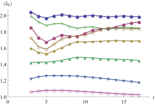
Figure 4: Senior eigenvalue smoothed over the period 4 of the system-specific oscillations for $\Delta J=0.1,\,0.2,\,0.3,\,0.4,\,0.5,\,0.6,\,0.7,\,\pi/4$ in the order upwards at the left border of the plot.

One sees that the two lowest curves ($\Delta J=0.1$ and $0.2)$ tend to go down such that ergodic behavior can be expected at larger times. The uppermost curve, practically constant at the level $\lambda=2,$ corresponds to the trivially localized case of non-interacting spins. As regards to other values of $\Delta J$ the large-time behavior predictions are not possible from these data. What strikes the eye is the irregularity of the behavior of the curves with $\Delta J=0.5,0.6,0.7$; they cross and change their relative positions at the right border of the plot compared with its left border. By different methods in Braun a transition of the KIC from ergodicity to localization occurring at $\Delta J=0.58$ was found; below we shall see a direct evidence of that transition.

V Large times, all $J$: indirect estimate of $\lambda_{0}$

By ”large” we mean here times of the order of the Heisenberg time $T_{H}=2^{N}$. We find it numerically most effective to estimate $\lambda_{0}\left(t\right)$ from the numerically calculated spectral form factor for several consecutive chain lengths $N$. It can be done if $\lambda_{0}\left(t\right)$ is separated by a gap from all others; we found in Ref. Braun that this is true at least in the limits of weak interaction and for small times for all non-zero $\Delta J$. Then for sufficiently large $N$ the form factor will be dominated by that single eigenvalue of the double dual operator growing exponentially with $N,$

$$K_{N}\left(t\right)\approx\left[\lambda_{0}\left(t\right)/2\right]^{N}$$ (17)

which corresponds to the localized regime. We showed in Ref. Braun that such a behavior follows if the system splits into independent subsystems. The gap between $\lambda_{0}\left(t\right)$ and the other eigenvalues of the double dual operator depends on time; if it shrinks to zero that estimate ceases to be true. On the other hand, in the ergodic limit the form factor obeys the GOE prediction, $K_{N}^{\rm{GOE}}(t)=2t/2^{N}-2\left(t/2^{N}\right)^{2}+\ldots$ ; at large $N$ the form factor is then practically $N-$independent apart from the trivial scaling with $T_{H.}=2^{N}$.

We now calculate the ratio,

$$\lambda_{0,N}\left(t\right)=\frac{2K_{N}\left(t\right)}{K_{N-1}\left(t\right)}$$ (18)

for sufficiently large $N$. If the chain is in the localized domain and (17) is applicable the result must be close to the $N-$independent $\lambda_{0}\left(t\right)$. That can be checked by comparison of the empirical $\lambda_{0,N}\left(t\right)$ and $\lambda_{0,N-1}\left(t\right)$; if these are not too different we achieved convergence in $N$ and can assume,

$$\lambda_{0}\left(t\right)\approx\lambda_{0,N}\left(t\right)\approx\lambda_{0,N-1}\left(t\right),$$

with the accuracy increasing with $N$.

We used that approach calculating the form factor of the KIC with $N=11-15$; the averaging was performed over 1000 disorder realizations. Consider, e. g. the result for $\Delta J=0.4$ in Fig. 5 where $\lambda_{0,12}\left(t\right)$ (red), $\lambda_{0,13}\left(t\right)$ (black) and $\lambda_{0,14}\left(t\right)$ (magenta) are depicted. The three dashed straight lines passing through the origin indicate that $\lambda_{0,N}(t)$ calculated for spectra obeys the GOE statistics,

$$\lambda_{0,N}^{\mathrm{GOE}}=\frac{2K_{N}^{\mathrm{GOE}}\left(t\right)}{K_{N-1}^{\mathrm{GOE}}\left(t\right)}=1+\frac{t}{2^{N}}+\ldots$$ (19)

for $N=12,13,14$. All three curves first go down following, apart from a small initial stretch, an almost straight line practically the same for all $N$ considered. Therefore they provide a sufficiently accurate approximation for the eigenvalue $\lambda_{0}\left(t\right)$ in that interval of times. At larger times the three curves diverge approaching their ”own” GOE lines: they first curve up and later merge with $\lambda_{0,N}^{\mathrm{GOE}}$ signaling the transition from the localized regime to ergodicity.

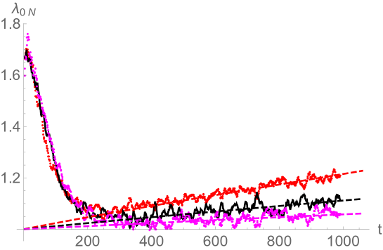
Figure 5: Approximate $\lambda_{0,N}(t)$ against time obtained as ratio of form factors of chains with 12 to 11 spins (red), 13 to 12 spins (black) and 14 to 13 spins (magenta), case $\Delta J=0.4$ with the corresponding GOE predictions (dashed lines).

The overall plot of $\lambda_{0,N}(t)$ with two almost straight stretches at the ends reminds of a hyperbola; in fact fitting them with a hyperbola one of whose asymptotes coincides with $\lambda_{0,N}^{\rm{GOE}}$ proved to be fairly accurate, see appendix C.

The GOE limit line approaches $\lambda=1$ with the increase of $N$. Extrapolating to $N\rightarrow\infty$ we can thus conjecture that the exact $\lambda_{0}\left(t\right)$ consists of the straight line with the negative slope insignificantly different from that of $\lambda_{0,12/13/14}\left(t\right)$. If we neglect the transition zone between the two regimes the overall plot of $\lambda_{0}\left(t\right)$ thus predicted consists of two straight lines and can be viewed as a degenerate hyperbola.

The family of similar plots of $\lambda_{0,N}(t)$ for several values of $\Delta J$ is shown in Fig. 6, with $a,b,c$ standing for $\Delta J=0.4,0.5,0.6$, respectively and the color indicating the value of $N$. In all cases there is good agreement between $\lambda_{0,N}(t)$ with $N=12-15$ at the descending stretch; at larger times the curves merge with the respective $\lambda_{0,N}^{\mathrm{GOE}},\quad N=12-15$. The negative slope of the decreasing stretch tends after a decay for small $t$ (see Figs. 2,3) to zero with the growth of $\Delta J$ and disappears for $\Delta J\geq 0.6$ .

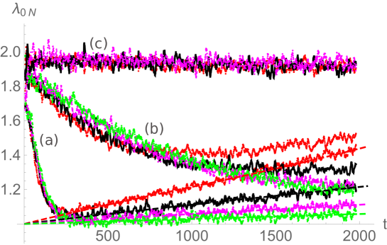
Figure 6: Plots of $\lambda_{0,N}(t)$ against time for $\Delta J=0.4(a),0.5(b),0.6(c)$ with $N=12$ (red), $13$ (black), $14$ (magenta) and $15$ (green). For a given $\Delta J$ the descending parts of the curves with different $N$ practically coincide indicating convergence in $N$. For larger times the plots tend to the respective GOE limits. For $\Delta J=0.6$ (beyond the localization threshold) the plots are horizontal

A more detailed analysis shows that zeroing of the slope occurs at the critical value $\Delta J=\Delta J_{c}\approx 0.58$. It agrees with our previous finding for the localization threshold in the KIC based on the spacing ratio statistics and the entanglement entropy Braun . Therefore we determined the slope of the initial linear stretch of $\lambda_{0,13}\left(t\right)$ as function of $\Delta J$ by fitting $\lambda_{0,13}\left(t\right)$ by hyperbolas (see appendix C) and calculated $d\lambda_{0}/dt$ at $t=0.$ The results are shown in Fig. 7.

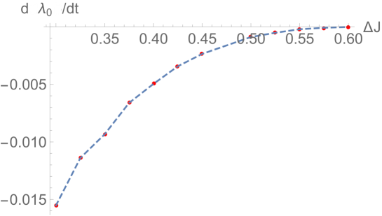
Figure 7: Slope of the linear stretch of $\lambda_{0}(t)$ against $\Delta J$

The curve smoothly approaches zero at $\Delta J\approx 0.58$ and stays zero at larger $\Delta J$ which reminds of the behavior in the vicinity of a critical point.

VI Estimate of the Thouless time

We want to use the results from the last section to give an estimate of the Thouless time of the system. It determines the time after that the system properties – here the spectral form factor – are described by RMT for large system size Thouless ; Santos . We use in this context the formula smoothly interpolating between the localized and the RMT regimes,

$$K_{N}\left(t\right)\approx K_{N}^{\rm{GOE}}\left(t\right)+\left[\lambda_{0}\left(t\right)^{N}-1\right]/2^{N}.$$ (20)

It follows then that

$$\lambda_{0}\left(t\right)\approx 2\left[K_{N}\left(t\right)-K_{N}^{\rm{GOE}}\left(t\right)+\frac{1}{2^{N}}\right]^{1/N}.$$ (21)

In the limit $N\rightarrow\infty$, time fixed, the GOE form factor tends to zero and we get the expression for $\lambda_{0}\left(t\right)=\lim_{N\rightarrow\infty}2\left[K_{N}\left(t\right)\right]^{1/N}$ of the localized regime; in the opposite limit of the ergodic regime we have $K_{N}\left(t\right)=K_{N}^{\rm{GOE}}\left(t\right)$ and $\lambda_{0}=1.$

The converged $\lambda_{0}\left(t\right)$ decreases from its maximum $\lambda_{m}=\lambda_{m}\left(\Delta J\right)$, $1<\lambda_{m}<2,$ reached at $t\sim 10$ to its ergodic regime value $\lambda_{0}=1$. In the regime of $\lambda_{0}\left(t\right)$ not very close to $1$ an exponential fitting turns out to be fairly accurate,

$$\lambda_{0}\left(t\right)=1+\left(\lambda_{m}-1\right)e^{-\eta t},$$ (22)

as shown in Fig. 8 for $N=15$ and $\Delta J=0.4$, $\Delta J=0.5$. As in that $t$ interval the corresponding curves for different $N$ look very similar we don’t show them in Fig. 8.

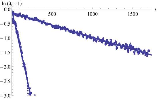
Figure 8: Logarithmic plot of $\lambda_{0}-1$ with fit curves for $N=15$ and $\Delta J=0.4$ (left curve) and $\Delta J=0.5$ (right curve).

The coefficient $\eta\left(\Delta J\right)$ decreases with the growth of $\Delta J$ tending to zero at about $\Delta J=\Delta J_{c}\approx 0.58$. For $\Delta J_{c}<$ $\Delta J\leq\pi/4$ the fitted $\lambda_{0}$ is time-independent increasing with the growth of $\Delta J\$reaching $2$ in the limit of non-interacting spins $\Delta J=\pi/4$.

The characteristic time $1/\eta$ of the decay of $\lambda_{0}\left(t\right)$ can be connected with the Thouless time $t_{Th}$ . Let us define it as the time at which the deviation of the system form factor from the RMT prediction $K_{N}^{\rm{GOE}}(t)$ becomes smaller than $K_{N}^{\rm{GOE}}(t)$ itself or, as follows from (20) when $\ln t\sim N\ln\lambda_{0}\left(t\right)$. Approximating $\ln\lambda_{0}\left(t\right)$ by $\left(\lambda_{m}-1\right)e^{-\eta t}$ (see (22)) we obtain that the Thouless time depends logarithmically on the system size,

$$t_{Th}\sim\frac{1}{\eta}\ln N.$$ (23)

The Thouless time determining the period until a quantity shows RMT features naturally depends on the quantity and the system considered. Given that Ref. Prosenarx considers here a quantity different from the spectral form factor explains the different ($N$ independent) scaling or the scaling with $N^{2}/D$ for a diffusive system with the diffusion constant $D$ ChalkerIII ; Prosenarx . A scaling of the Thouless with $\ln N$ was also predicted for large single-particle Hilbert spaces in Chalker ; ChalkerI and for $s=1/2$ in ProsenI ; ChalkerII for different systems by other methods. By the analysis in this section we generalize our results for the Thouless time valid in the perturbative regime of small $\Delta J$ to arbitrary $\Delta J$.

VII Conclusion

We studied the transition from ergodicity to localization in the KIC of $N$ spins $1/2$ in the presence of strong local disorder. Our tool was the double dual operator introduced in Prosen where it was used to prove ergodicity and RMT behavior of the KIC with parameters corresponding to the so called self-dual regime. We used it to probe the localization effects caused by deviations from self-duality considering that the behavior of the spectral form factor in the thermodynamic limit $N\gg 1$ is determined by the largest eigenvalue $\lambda_{0}\left(t\right)$ of the double dual operator $\mathcal{A}\left(t\right)$.

We calculated $\lambda_{0}(t)$ as function of the Ising constant $J$ in the interval from $\pi/4$ corresponding to self-duality, to $J=0$ corresponding to non-interacting spins, i. e., trivial localization. Several methods were used which gave overlapping result: First, for $J=0$ we obtained $\lambda_{0}(t)$ analytically and perturbatively for small $J$. Comparing it with the numerically computed $\lambda_{0}(t)$ for $t\leq 20$ we observe that despite a shrinking convergence of the perturbation theory with increasing $t$ it reproduces the structure observed in Ref. Braun in the vicinity of $J=0$ where the $\lambda_{0}(t)$ values for a sufficiently large $J$ oscillate around the ones for $J=0$. We also show that the eigenvalue $\lambda_{0}(t)$ dominating the spectral form factor for $J$ close to zero possesses the same symmetry as the dominant eigenvalue for small $t$ in the regime of $J$ close to $\pi/4$. Second, for times of the order of the Heisenberg time $T_{H}=2^{N}$ we estimated $\lambda_{0}\left(t\right)$ by extensive numerical simulations computing the spectral form factor of chains of up to $N\leq 15$ and extrapolating the result to an infinite chain thereby complementing our results in Ref. Braun only valid for small $t$ and $N$, respectively.

We observed here that the chain has two characteristic regimes: In the localized regime the eigenvalue $\lambda_{0}(t)>1$ is separated by a gap from all other eigenvalues of the double dual operator; the form factor has an exponential dependence on the number of spins. In the ergodic regime $\lambda_{0}\left(t\right)$ is for large $t$ close to unity and is the uppermost level of a narrow multiplet of $2t$ eigenvalues of $\mathcal{A}\left(t\right)$ extending the picture of a single dominant largest eigenvalue in the regime of small $t$ we found in Ref. Braun . The form factor coincides with the RMT predictions and is $N-$independent apart from the trivial scaling with $T_{H}$. Both regimes coexist if the deviation $\Delta J=\pi/4-J$ from self-duality is smaller than $\Delta J_{c}\approx 0.58$, namely we have localization with $\lambda_{0}\left(t\right)>1$ when $t$ is smaller than the Thouless time and ergodicity with $\lambda_{0}(t)\approx 1$ when $t$ is larger than the Thouless time. The latter time grows from $0$ at $\Delta J=0$ to infinity at $\Delta J=\Delta J_{c}$ and determines the transition in the thermodynamic limit. In the time interval below the Thouless time $\lambda_{0}\left(t\right)$ decays as a function of time, this decay tends to zero as $\Delta J$ approaches the critical value. For $\Delta J>\Delta J_{c}$ the eigenvalue $\lambda_{0}$ is time independent apart from the system-specific fluctuations.

There are various possibilities to extend these results: First, our perturbative results will probably allow to get an analytical expression for the spectral Lyapunov exponents in the symmetry block invariant under permutations and reflections in ChalkerI . Second, our present findings show that the behavior of the dominant eigenvalue $\lambda_{0}\left(t\right)$ of the double dual operator can be a useful localization witness in spin chains within the dual operator approach. It would be interesting to check that for other spin values and types of interactions.

Appendix A Symmetry properties of eigenvector to the eigenvalue of largest magnitude for $J=0$

According to Ref. Braun the dual operator in the absence of interaction is

$$\hat{W}\left(t\right) =\prod_{n=1}^{N}\hat{w}_{n}\,,$$ (24)

$$\hat{w}_{n} =\hat{w}_{I}\hat{w}_{n,b},$$

$$\left\langle\boldsymbol{\sigma}^{t}\left|\hat{w}_{I}\right|\boldsymbol{\sigma}^{\prime t}\right\rangle =\left.\exp\left(-iJ\sum_{k=1}^{t}\sigma_{k}\sigma_{k}^{\prime}\right)\right|_{J=0}=1,$$

$$\left\langle\boldsymbol{\sigma}^{t}\left|\hat{w}_{n,b}\right|\boldsymbol{\sigma}^{\prime t}\right\rangle =\delta_{\mathbf{\sigma}^{t}\mathbf{\sigma}}\exp\left(-ih_{n}\sum_{k=1}^{t}\sigma_{k}\right)\prod_{k=1}^{t}R_{\mathbf{\sigma}_{k}\sigma_{k+1}},$$

i. e., the Ising matrix $\hat{w}_{I}$ has all elements equal 1. It has a single non-zero eigenvalue equal to the matrix size $2^{t}$ corresponding to the eigenvector with all elements equal, i. e., the sum of all basis vectors in the dual space with equal coefficients; unnormalized it is

$$|\chi\rangle = \sum_{\sigma_{1},\sigma_{2},\ldots,\sigma_{t}=\pm 1}|\sigma_{1},\sigma_{2},\ldots,\sigma_{t}\rangle,$$ (25)

$$\langle\chi|\chi\rangle = 2^{t}.$$

Therefore $\hat{w}_{I}$ is simply,

$$\hat{w}_{I}=|\chi\rangle\langle\chi|$$ (26)

That state is invariant with respect to the cyclic shifts and reflections in the dual space the corresponding symmetry block we denoted in Ref. Braun by (0+). The local dual operator on the $n$-th spin is therefore,

$$\hat{w}_{n}=\sum_{\sigma}f_{n}(\boldsymbol{\sigma})|\chi\rangle\langle\boldsymbol{\sigma}|$$ (27)

with

$$f_{n}(\boldsymbol{\sigma})=\langle\chi|\boldsymbol{\sigma}\rangle\exp\left(-ih_{n}\sum_{k=1}^{t}\sigma_{k}\right)\prod_{k=1}^{t}R_{\sigma_{k}\sigma_{k+1}}.$$ (28)

We know that the operators $\hat{w}_{n}$ are block diagonal in the symmetrized basis set. However, $\hat{w}_{n}$ has only zero matrix elements in any symmetry block except (0+) because of the fully symmetric ket-vector $|\chi\rangle$. Hence all blocks of $\hat{w}_{n}$ except (0+) are zero and same refers to their product $\hat{W}$. In the operator $\mathcal{A}$ the only non-zero block is therefore (0+; 0+) such that any non-zero eigenvalue of $\mathcal{A}$ belongs to an eigenstate of highest symmetry.

Appendix B Perturbation theory

Here we aim at obtaining a perturbative expression in $J$ for $\lambda_{0}(t)$. Therefore we expand the form factor (2) perturbatively for small coupling $J$. In this context we need the linear and the quadratic orders in $J$ of ${\rm Tr}\hat{U}^{t}$. The linear order is given by

$$t{\rm Tr}\left[\left(iJ\sum_{n=1}^{N}\sigma_{n}^{z}\sigma_{n+1}^{z}\right)\prod_{n=1}^{N}\hat{u}_{n}^{t}\right]$$

$$= t{\rm Tr}\left[\left(iJ\sum_{n=1}^{N}\sigma_{n}^{z}\sigma_{n+1}^{z}\right)\prod_{n=1}^{N}e^{it\gamma_{n}{\bf{e}}_{n}{\boldsymbol{\sigma}}_{n}/2}\right]$$

$$= -itJ2^{N}\left[\sum_{n=1}^{N}\frac{\sin(t\gamma_{n}/2)}{\sqrt{2+\cot^{2}h_{n}}}\frac{\sin(t\gamma_{n+1}/2)}{\sqrt{2+\cot^{2}h_{n+1}}}\prod_{i=1,i\neq n,n+1}^{N}\cos(t\gamma_{i}/2)\right].$$

The square roots in the last line result from the $z$-components of the normal vectors ${\bf{e}}_{n}$, ${\bf{e}}_{n+1}$ of the rotation matrix $\hat{u}_{n}$. The corresponding contribution to the spectral form factor in linear order of $J$ that follows from the expression above is zero because (B) is purely imaginary.

For the quadratic order two further contributions are of relevance. At first one of the $t$ $\hat{U}_{I}$’s in Eq. (1) entering the ${\rm Tr}\hat{U}^{t}$ can be expanded at quadratic order in $J$ leading to the contribution to ${\rm Tr}\hat{U}^{t}$

$$-\frac{J^{2}t}{2}{\rm Tr}\left[\sum_{n,m=1}^{N}\sigma_{n}^{z}\sigma_{n+1}^{z}\sigma_{m}^{z}\sigma_{m+1}^{z}\prod_{n=1}^{N}\hat{u}_{n}^{t}.\right]$$ (30)

To proceed we need to distinguish in the last equation the different cases

1. $n$, $n+1$, $m$, $m+1$ all different

2. $n=m$

3. $n=m-1$, $n=m+1$.

Summing up the contributions from all the cases we obtain the corresponding contribution to ${\rm Tr}\hat{U}^{t}$

$$-J^{2}t2^{N-1}\left[\sum_{n\neq m\neq m+1\neq n+1}\frac{\sin(t\gamma_{n}/2)}{\sqrt{2+\cot^{2}h_{n}}}\frac{\sin(t\gamma_{n+1}/2)}{\sqrt{2+\cot^{2}h_{n+1}}}\frac{\sin(t\gamma_{m}/2)}{\sqrt{2+\cot^{2}h_{m}}}\right.$$

$$\left.\frac{\sin(t\gamma_{m+1}/2)}{\sqrt{2+\cot^{2}h_{m+1}}}\prod_{i\neq n\neq m\neq n+1\neq m+1}\cos(t\gamma_{i}/2)+N\prod_{i=1}^{N}\cos(t\gamma_{i}/2)\right.$$

$$\left.-2\sum_{n}\frac{\sin(t\gamma_{n}/2)}{\sqrt{2+\cot^{2}h_{n}}}\frac{\sin(t\gamma_{n+2}/2)}{\sqrt{2+\cot^{2}h_{n+2}}}\prod_{i\neq n\neq n+2}\cos(t\gamma_{i}/2)\right].$$ (31)

Furthermore we also need to expand two of the $t$ $\hat{U}_{I}$’s up linear order in $J$ yielding

$$-\frac{J^{2}t}{2}\sum_{\tau=1}^{t-1}{\rm Tr}\left[\sum_{nm}\sigma_{n}^{z}\sigma_{n+1}^{z}\prod_{i}\hat{u}_{i}^{\tau}\sigma_{m}^{z}\sigma_{m+1}^{z}\prod_{i}\hat{u}_{i}^{t-\tau}\right]$$ (32)

that can be transformed into

$$-\frac{J^{2}t}{2}\sum_{\tau=1}^{t-1}{\rm Tr}\left[\sum_{nm}\sigma_{n}^{z}\sigma_{n+1}^{z}\sigma_{m}^{z}\sigma_{m+1}^{z}\prod_{i\neq m\neq m+1}\hat{u}_{i}^{t}\hat{\overline{u}}_{m}^{\tau}\hat{\overline{u}}_{m+1}^{\tau}\hat{u}_{m}^{(t-\tau)}\hat{u}_{m+1}^{(t-\tau)}\right],$$ (33)

where $\hat{\overline{u}}_{m}^{\tau}=\cos(\tau\gamma_{m}/2)-(in_{m}^{x}\sigma_{m}^{x}+in_{m}^{y}\sigma_{m}^{y}-in_{m}^{z}\sigma_{m}^{z})\sin(\tau\gamma_{m}/2)$ and an analogous definition of $\hat{\overline{u}}_{m+1}^{\tau}$. Again distinguishing the cases

1. $n$, $n+1$, $m$, $m+1$ all different

2. $n=m$

3. $n=m-1$, $n=m+1$

we get the following contribution to ${\rm Tr}\hat{U}^{t}$

$$-J^{2}t2^{N-1}\sum_{\tau=1}^{t-1}\left[\sum_{n\neq m\neq m+1\neq n+1}\frac{\sin t\gamma_{n}/2}{\sqrt{2+\cot^{2}h_{n}}}\frac{\sin t\gamma_{m+1}/2}{\sqrt{2+\cot^{2}h_{m+1}}}\frac{\sin t\gamma_{m}/2}{\sqrt{2+\cot^{2}h_{m}}}\frac{\sin t\gamma_{n+1}/2}{\sqrt{2+\cot^{2}h_{n+1}}}\right.$$

$$\left.\prod_{i\neq n\neq m\neq n+1\neq m+1}\cos\frac{t\gamma_{i}}{2}+\sum_{m}\left(\cos\frac{\tau\gamma_{m}}{2}\cos\frac{(t-\tau)\gamma_{m}}{2}+\sin\frac{\tau\gamma_{m}}{2}\right.\right.$$

$$\left.\left.\sin\frac{(t-\tau)\gamma_{m}}{2}\frac{\cot^{2}h_{m}}{2+\cot^{2}h_{m}}\right)\left(\cos\frac{\tau\gamma_{m+1}}{2}\cos\frac{(t-\tau)\gamma_{m+1}}{2}+\sin\frac{\tau\gamma_{m+1}}{2}\right.\right.$$

$$\left.\left.\sin\frac{(t-\tau)\gamma_{m+1}}{2}\frac{\cot^{2}h_{m+1}}{2+\cot^{2}h_{m+1}}\right)\prod_{i\neq m,m+1}\cos\frac{t\gamma_{i}(h)}{2}-\sum_{m}\left(\cos\frac{\tau\gamma_{m}}{2}\cos\frac{(t-\tau)\gamma_{m}}{2}\right.\right.$$

$$\left.\left.+\sin\frac{\tau\gamma_{m}}{2}\sin\frac{(t-\tau)\gamma_{m}}{2}\frac{\cot^{2}h_{m}}{2+\cot^{2}h_{m}}\right)\frac{\sin t\gamma_{m-1}/2}{\sqrt{2+\cot^{2}h_{m-1}}}\frac{\sin t\gamma_{m+1}/2}{\sqrt{2+\cot^{2}h_{m+1}}}\right.$$

$$\left.\prod_{i\neq m\neq m-1\neq m+1}\cos\frac{t\gamma_{i}}{2}-\sum_{m}\left(\cos\frac{\tau\gamma_{m+1}}{2}\cos\frac{(t-\tau)\gamma_{m+1}}{2}\right.\right.$$

$$\left.\left.+\sin\frac{\tau\gamma_{m+1}}{2}\sin\frac{(t-\tau)\gamma_{m+1}}{2}\frac{\cot^{2}h_{m+1}}{2+\cot^{2}h_{m+1}}\right)\frac{\sin t\gamma_{m}/2}{\sqrt{2+\cot^{2}h_{m}}}\frac{\sin t\gamma_{m+2}/2}{\sqrt{2+\cot^{2}h_{m+2}}}\right.$$

$$\left.\prod_{i\neq m\neq m+1\neq m+2}\cos\frac{t\gamma_{i}}{2}\right].$$ (34)

Now we can obtain the contribution to the spectral form factor that is of quadratic order in $J$. To summarize, we just derived an expansion of ${\rm Tr}\hat{U}^{t}$ in $J$

$${\rm Tr}\hat{U}^{t}=\left({\rm Tr}\hat{U}^{t}\right)_{(0)}+J\left({\rm Tr}\hat{U}^{t}\right)_{(1)}+J^{2}\left({\rm Tr}\hat{U}^{t}\right)_{(2)}+\dots,$$ (35)

where the subscripts in the last equation indicate the order in $J$. This allows to obtain the contribution to $K_{N}(t)$ quadratic in $J$

$$\left({\rm Tr}\hat{U}^{t}\right)_{(1)}\left({\rm Tr}\hat{U}^{t}\right)_{(1)}^{*}+\left({\rm Tr}\hat{U}^{t}\right)_{(2)}\left({\rm Tr}\hat{U}^{t}\right)_{(0)}^{*}+\left({\rm Tr}\hat{U}^{t}\right)_{(0)}\left({\rm Tr}\hat{U}^{t}\right)_{(2)}^{*}.$$ (36)

Summing all these terms we get for the contribution quadratic in $J$ to $K_{N}(t)$

$$t^{2}J^{2}4^{N}\left[\sum_{n}\frac{\sin^{2}t\gamma_{n}/2}{2+\cot^{2}h_{n}}\frac{\sin^{2}t\gamma_{n+1}/2}{2+\cot^{2}h_{n+1}}\prod_{i\neq n\neq n+1}\cos^{2}\frac{t\gamma_{i}}{2}\right.$$

$$\left.+2\sum_{n}\frac{\sin t\gamma_{n}/2}{\sqrt{2+\cot^{2}h_{n}}}\frac{\sin^{2}t\gamma_{n+1}/2}{2+\cot^{2}h_{n+1}}\frac{\sin t\gamma_{n+2}/2}{\sqrt{2+\cot^{2}h_{n+2}}}\prod_{i\neq n\neq n+1\neq n+2}\right.$$

$$\left.\cos^{2}\frac{t\gamma_{i}}{2}\cos\frac{t\gamma_{n}}{2}\cos\frac{t\gamma_{n+2}}{2}-\frac{N}{T}\prod_{i}\cos^{2}\frac{t\gamma_{i}}{2}+\frac{2}{t}\right.$$

$$\left.\sum_{n}\frac{\sin t\gamma_{n}/2}{\sqrt{2+\cot^{2}h_{n}}}\frac{\sin t\gamma_{n+2}/2}{\sqrt{2+\cot^{2}h_{n+2}}}\prod_{i\neq n\neq n+2}\cos^{2}\frac{t\gamma_{i}}{2}\cos\frac{t\gamma_{n}}{2}\cos\frac{t\gamma_{n+2}}{2}\right.$$

$$\left.-\frac{1}{t}\sum_{\tau=1}^{t-1}\sum_{n}\left(\cos\frac{\tau\gamma_{n}}{2}\cos\frac{(t-\tau)\gamma_{n}}{2}+\sin\frac{\tau\gamma_{n}}{2}\sin\frac{(t-\tau)\gamma_{n}}{2}\frac{\cot^{2}h_{n}}{2+\cot^{2}h_{n}}\right)\right.$$

$$\left.\left(\cos\frac{\tau\gamma_{n+1}}{2}\cos\frac{(t-\tau)\gamma_{n+1}}{2}+\sin\frac{\tau\gamma_{n+1}}{2}\sin\frac{(t-\tau)\gamma_{n+1}}{2}\frac{\cot^{2}h_{n+1}}{2+\cot^{2}h_{n+1}}\right)\right.$$

$$\left.\prod_{i\neq n\neq n+1}\cos^{2}\frac{t\gamma_{i}}{2}\cos\frac{t\gamma_{n}}{2}\cos\frac{t\gamma_{n+1}}{2}+\frac{2}{t}\sum_{n}\left(\cos\frac{\tau\gamma_{n}}{2}\cos\frac{(t-\tau)\gamma_{n}}{2}\right.\right.$$

$$\left.\left.+\sin\frac{\tau\gamma_{n}}{2}\sin\frac{(t-\tau)\gamma_{n}}{2}\frac{\cot^{2}h_{n}}{2+\cot^{2}h_{n}}\right)\frac{\sin t\gamma_{n-1}/2}{\sqrt{2+\cot^{2}h_{n-1}}}\frac{\sin t\gamma_{n+1}/2}{\sqrt{2+\cot^{2}h_{n+1}}}\right.$$

$$\left.\prod_{i\neq n\neq n-1\neq n+1}\cos^{2}\frac{t\gamma_{i}}{2}\cos\frac{t\gamma_{n}}{2}\cos\frac{t\gamma_{n-1}}{2}\cos\frac{t\gamma_{n+1}}{2}\right].$$ (37)

Using the relation

$$\int_{0}^{\pi}dh\cos\frac{t\gamma_{i}}{2}\sin\frac{t\gamma_{i}}{2}=0$$ (38)

with $\gamma_{i}$ given in Eq. (5) and the result in Eq. (6) we can simplify (B) to

$$tJ^{2}N\left[t\left(\frac{4}{\pi}\int_{0}^{\pi}dh\frac{\sin^{2}t\gamma/2}{2+\cot^{2}h}\right)^{2}\left(2+\frac{(-1)^{q}(2p-1)!!}{(2p)!!}\right)^{N-2}\right.$$

$$\left.-\left(2+\frac{(-1)^{q}(2p-1)!!}{(2p)!!}\right)^{N}\right.$$

$$\left.-\sum_{\tau=1}^{t-1}\left(\frac{4}{\pi}\int_{0}^{\pi}dh\left(\cos\frac{\tau\gamma}{2}\cos\frac{(t-\tau)\gamma}{2}+\sin\frac{\tau\gamma}{2}\sin\frac{(t-\tau)\gamma}{2}\frac{\cot^{2}h}{2+\cot^{2}h}\right)\right.\right.$$

$$\left.\left.\cos\frac{t\gamma}{2}\right)^{2}\left(2+\frac{(-1)^{q}(2p-1)!!}{(2p)!!}\right)^{N-2}\right].$$ (39)

with $q=[(t+1)/2]$ and $p=[t/2]$. This implies we can rewrite the spectral form factor as

$$K_{N}(t)=\lambda_{0}(t)^{N}\left[1+\frac{NJ^{2}f(t)}{\lambda_{0}^{2}}\right]$$ (40)

with a function $f(t)$ that can be read off from Eq. (B) and

$$\lambda_{0}(t)=\left(2+\frac{(-1)^{q}(2p-1)!!}{(2p)!!}\right).$$ (41)

Using $1+Nx\approx(1+x)^{N}$ in the limit $N\to\infty$ we get for the spectral form factor

$$K_{N}(t)=\left[\lambda_{0}(t)\left(1+\frac{J^{2}f(T)}{\lambda_{0}(t)^{2}}\right)\right]^{N}.$$ (42)

From this equation we can extract by means of $K_{N}(t)=\lambda(t)^{N}$ an expression for $\lambda(t)$

$$\lambda(t)=\lambda_{0}(t)\left(1+\frac{J^{2}f(t)}{\lambda_{0}(t)^{2}}\right)$$ (43)

that yields in detail

$$\lambda(t) = \lambda_{0}(t)+\frac{tJ^{2}}{\lambda_{0}(t)}\left[T\left(\frac{4}{\pi}\int_{0}^{\pi}dh\frac{\sin^{2}t\gamma/2}{2+\cot^{2}h}\right)^{2}-\lambda_{0}(t)^{2}\right.$$ (44)

$$\left.-\sum_{\tau=1}^{t-1}\left(\frac{4}{\pi}\int_{0}^{\pi}dh\left(\cos\frac{\tau\gamma}{2}\cos\frac{(t-\tau)\gamma}{2}+\sin\frac{\tau\gamma}{2}\sin\frac{(t-\tau)\gamma}{2}\frac{\cot^{2}h}{2+\cot^{2}h}\right)\right.\right.$$

$$\left.\left.\cos\frac{t\gamma}{2}\right)^{2}\right].$$

These integrals can be calculated by residual integration in terms of the generalized binomial coefficients. The final result is given as expression (13) in the main text.

The expression (13) still contains one sum with respect to $\tau$ that we now want to perform in the limit of large $t$. We will concentrate on the smooth part ignoring the contributions from oscillations with period four. In this context we use the method of stationary phase assuming $\tau$, $t$, and $t-\tau$ to be large. We note that this is in principle not fulfilled as not for all terms in the $\tau$-sum $\tau$ and $t-\tau$ can be large, but we found by comparison with numerics that our approximation is already quite good for $t\approx 20$. In a first step we rewrite

$$\sum_{\tau=1}^{t-1}\left(\frac{4}{\pi}\int_{0}^{\pi}dh\left(\cos\frac{\tau\gamma(h)}{2}\cos\frac{(t-\tau)\gamma(h)}{2}+\sin\frac{\tau\gamma(h)}{2}\sin\frac{(t-\tau)\gamma(h)}{2}\frac{\cot^{2}h}{2+\cot^{2}h}\right)\cos\frac{t\gamma(h)}{2}\right)^{2}$$ (45)

$$= \sum_{\tau=1}^{t-1}\frac{1}{\pi^{2}}\left[\int_{0}^{\pi}dh\left(\cos t\gamma(h)+1\right)\frac{2}{2+\cot^{2}h}+\left(\cos\tau\gamma(h)+\cos(t-\tau)\gamma(h)\right)\frac{2+2\cot^{2}h}{2+\cot^{2}h}\right]^{2}.$$

Taking into account that $\gamma(h)$ becomes stationary at $h=0$ and at $h=\pi$ we get for the last expression

$$\sum_{\tau=1}^{t-1}\frac{1}{\pi}\left[\sqrt{\frac{1}{\tau}}\left(\cos\left(\frac{\tau\pi}{2}+\frac{\pi}{4}\right)+\cos\left(\frac{3\tau\pi}{2}-\frac{\pi}{4}\right)\right)+\sqrt{\frac{1}{t-\tau}}\left(\cos\left(\frac{(t-\tau)\pi}{2}+\frac{\pi}{4}\right)\right.\right.$$

$$\left.\left.+\cos\left(\frac{3(t-\tau)\pi}{2}-\frac{\pi}{4}\right)\right)+\sqrt{\pi}(2-\sqrt{2})\right]^{2},$$ (46)

where we evaluated the part of the integral in (45) independent of $t$ and $\tau$ exactly and the rest within the stationary phase approximation. In the next step we want to evaluate the latter expression in the limit of large $t$ neglecting additionally contributions rapidly oscillating as a function of $t$. Calculating the square in (B) we get the following contributions: First,

$$(2-\sqrt{2})^{2}(t-1).$$ (47)

Second, the mixed term from the square in (B) yields

$$\sum_{\tau=1}^{t-1}\frac{4(2-\sqrt{2})}{\sqrt{\pi\tau}}\left[\cos\left(\frac{\tau\pi}{2}+\frac{\pi}{4}\right)+\cos\left(\frac{3\pi\tau}{2}-\frac{\pi}{4}\right)\right]$$

$$=\frac{4(\sqrt{2}-1)}{\sqrt{\pi}}\left[(2-\sqrt{2})\zeta[1/2]-i^{t}\left(\zeta[1/2,t/4]-\zeta[1/2,(t+2)/4]\right)\right.$$ (48)

$$\left.-\zeta[1/2,1/4]+\zeta[1/2,3/4]-i^{t}\left(\zeta[1/2,1/4(3+t)]-\zeta[1/2,(1+t)/4]\right)\right]$$

for $t$ even and for $t$ odd

$$\sum_{\tau=1}^{t-1}\frac{4(2-\sqrt{2})}{\sqrt{\pi\tau}}\left[\cos\left(\frac{\tau\pi}{2}+\frac{\pi}{4}\right)+\cos\left(\frac{3\pi\tau}{2}-\frac{\pi}{4}\right)\right]$$

$$=\frac{4(\sqrt{2}-1)}{\sqrt{\pi}}\left[(2-\sqrt{2})\zeta[1/2]+\sin[\pi t/2]\left(\zeta[1/2,(1+t)/4]-\zeta[1/2,(3+t)/4]\right)\right.$$ (49)

$$\left.-\zeta[1/2,1/4]+\zeta[1/2,3/4]+(-1)^{[t/2]}\left(\zeta[1/2,1/4(1+2[t/2])]-\zeta[1/2,(3+2[t/2])/4]\right)\right],$$

where the last lines in the two last equations are obtained from mathematica with the Hurwitz zeta function $\zeta[a,s]$ and the Riemann zeta function $\zeta[s]$. As these functions tend to zero for $t\to\infty$ we get for the last expression in that limit

$$\frac{4(\sqrt{2}-1)}{\sqrt{\pi}}\left[(2-\sqrt{2})\zeta[1/2]-\zeta[1/2,1/4]+\zeta[1/2,3/4]\right].$$ (50)

Third, the last contributions results from the square of the cosine functions in (B). Neglecting all contributions that decay with $t$ we get by mathematica

$$\sum_{\tau=1}^{t-1}\frac{2}{\pi\tau}\left[\cos\left(\frac{\tau\pi}{2}-\frac{\pi}{4}\right)+\cos\left(\frac{3\pi\tau}{2}-\frac{\pi}{4}\right)\right]^{2}=\frac{4}{\pi}\left(\gamma+\ln t\right)$$ (51)

with the Euler constant $\gamma$. The mixed term

$$\sum_{\tau=1}^{t-1}\frac{2}{\pi\sqrt{\tau(t-\tau)}}\left[\cos\left(\frac{\tau\pi}{2}-\frac{\pi}{4}\right)+\cos\left(\frac{3\pi\tau}{2}-\frac{\pi}{4}\right)\right]$$

$$\left[\cos\left(\frac{(t-\tau)\pi}{2}-\frac{\pi}{4}\right)+\cos\left(\frac{3\pi(t-\tau)}{2}-\frac{\pi}{4}\right)\right]$$ (52)

oscillates around zero as a function of $t$, see Fig. 9 and thus does not contribute.

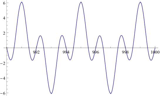
Figure 9: Contribution (B) as a function of $t$.

To obtain an overall expression for Eq. (44) averaged with respect to $t$ we also need to analyze the first term there in the curved bracket. In the limit of large $t$ we get

$$\frac{4}{\pi}\int_{0}^{\pi}dh\frac{\sin^{2}t\gamma/2}{2+\cot^{2}h}=2-\sqrt{2}.$$ (53)

To summarize, the results in Eqs. (53,51,50,47,7) finally imply the relation (16) in the main part.

Appendix C Fitting by a hyperbola

The empirical curves of $\lambda_{0,N}\left(t\right)$ remind of a hyperbola approaching straight lines on both edges and a curved arc between them. Therefore we used for fitting a 3-parameter function representing a hyperbola with one of whose asymptotes coinciding with the GOE prediction $\lambda_{0,N}^{GOE}\left(t\right)$ (19),

$$\lambda_{fit,N}\left(t\right) =-b-2at$$

$$+\sqrt{b^{2}-4ac+2\left(1+b\right)\left(2a+2^{-N}\right)t+\left(2a+2^{-N}\right)^{2}t^{2}}$$

with $a,b,c$ the fitting parameters. That fitting worked well for all $\Delta J$. As an example see Fig. 10 where we show $\lambda_{0,13}\left(t\right),\Delta J=0.4,$ (blue dots) and the fitting curve (red line).

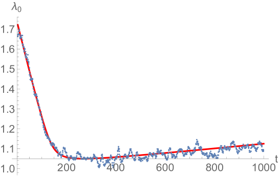
Figure 10: $\lambda_{0,13}$ against time (blue dots), fitting by a hyperbola (red line)

References

- (1) Y.Y. Atas, E. Bogomolny, J. Phys. A 47, 335201 (2014).
- (2) J.P. Keating, N. Linden, H.J. Wells, Commun. Math. Phys. 338, 81 (2015).
- (3) S. Czischek, M. Gärttner, M. Oberthaler, M. Kastner, T. Gasenzer, Quantum Science and Technology, 4, 014006 (2018).
- (4) A. Krishnan, M. Schmitt, R. Moessner, M. Heyl, Phys. Rev. A 100, 022125 (2019).
- (5) P. Ponte, Z. Papić, F. Huveneers, D.A. Abanin, Phys. Rev. Lett. 114, 140401 (2015).
- (6) M. Žnidarič, A. Scardicchio, V.K. Varma, Phys. Rev. Lett. 117, 040601 (2016).
- (7) S. Langer, F. Heidrich-Meisner, J. Gemmer, I.P. McCulloch, U. Schollwöck, Phys. Rev. B 79, 214409 (2009).
- (8) R. Steinigeweg, J. Gemmer, Phys. Rev. B 80, 184402 (2009).
- (9) T. Engl, J. Dujardin, A. Argüelles, P. Schlagheck, K. Richter, and J.D. Urbina, Phys. Rev. Lett. 112, 140403 (2014).
- (10) R. Dubertrand, S. Müller, New J. of Physics, 18, 033009 (2016).
- (11) T. Herrmann, M.F.I. Kieler, F. Fritzsch, A. Bäcker, Phys. Rev. E 101, 022221 (2020).
- (12) F. Haake, S. Gnutzmann, M. Kus, Quantum Signatures of Chaos, 4th Ed., Springer (2018).
- (13) H.-J. Stöckmann, Quantum Chaos-an introduction, Cambridge University Press (2008).
- (14) M. Akila, D. Waltner, B. Gutkin, T. Guhr, J. Phys. A 49, 375101 (2016).
- (15) B. Bertini, P. Kos, T. Prosen, Phys. Rev. Lett. 121, 264101 (2018).
- (16) A. Chan, A. De Luca, J.T. Chalker, Phys. Rev. Lett. 121, 060601 (2018).
- (17) A. Chan, A. De Luca, J.T. Chalker, Phys. Rev. Research 3, 023118 (2021).
- (18) P. Braun, D. Waltner, M. Akila, B. Gutkin, T. Guhr, Phys. Rev. E 101, 052201 (2020).
- (19) A. Flack, B. Bertini, T. Prosen, Phys. Rev. Research 2, 043403 (2020).
- (20) B. Bertini, P. Kos, T. Prosen, Phys. Rev. X 9, 021033 (2019).
- (21) R. Pal and A. Lakshminarayan, Phys. Rev. B 98, 174304 (2018).
- (22) S. Gopalakrishnan, A. Lamacraft, Phys. Rev. B, 100, 064309, (2019).
- (23) B. Gutkin, P. Braun, M. Akila, D. Waltner, T. Guhr, Phys. Rev. B 102, 174307 (2020).
- (24) B. Bertini, P. Kos, T. Prosen, Phys. Rev. Lett. 123, 210601 (2019).
- (25) P.W. Claeys, A. Lamacraft, Phys. Rev. Research 2, 033032 (2020).
- (26) M. Akila, D. Waltner, B. Gutkin, P. Braun, T. Guhr, Phys. Rev. Lett. 118, 164101 (2017).
- (27) S.J. Garratt, J.T. Chalker, arXiv:2008.01697.
- (28) M.L. Mehta, Random Matrices, Academic Press (2014).
- (29) T. Guhr, A. Müller-Groeling, H.A. Weidenmüller, Phys. Rep. 299, 189 (1998).
- (30) T. Prosen, Prog. Theor. Phys. Suppl. 139, 191 (2000); Phys. Rev. E 65, 036208 (2002); J. Phys. A 40, 7881 (2007).
- (31) B. Bertini, P. Kos, T. Prosen, Phys. Rev. Lett. 126, 190601 (2021).
- (32) In fact , plus some number-theoretical exceptions, but such details will be of not interest in our crude approach.
- (33) D.J. Thouless, Phys. Rev. Lett. 39, 1167 (1977).
- (34) M. Schiulaz, E.J. Torres-Herrera, L.F. Santos, Phys. Rev. B 99, 174313 (2019).
- (35) A.J. Friedman, A. Chan, A. De Luca, J.T. Chalker, Phys. Rev. Lett. 123, 210603 (2019).
- (36) P. Kos, M. Ljubotina, T. Prosen, Phys. Rev. X 8, 021062 (2018).