CutFEM Based on Extended Finite Element Spaces

Abstract

We develop a general framework for construction and analysis of discrete extension operators with application to unfitted finite element approximation of partial differential equations. In unfitted methods so called cut elements intersected by the boundary occur and these elements must in general by stabilized in some way. Discrete extension operators provides such a stabilization by modification of the finite element space close to the boundary. More, precisely the finite element space is extended from the stable interior elements over the boundary in a stable way which also guarantees optimal approximation properties. Our framework is applicable to all standard nodal based finite elements of various order and regularity. We develop an abstract theory for elliptic problems and associated parabolic time dependent partial differential equations and derive a priori error estimates. We finally apply this to some examples of partial differential equations of different order including the interface problems, the biharmonic operator and the sixth order triharmonic operator.

1 Introduction

Building on ideas around unfitted finite element methods using Nitsche’s method and boundary stabilization terms from the papers [16, 18, 17, 3, 5, 8, 9, 19, 24], the framework of cut finite element methods was proposed in [6]. The main idea was to use computational meshes and finite element spaces that were independent of the geometry of the physical problem. Both the partial differential equation and the geometry were then defined through the finite element variational form. In particular, Nitsche’s method was used to impose boundary and interface conditions and certain stabilization terms, so called, ghost penalty terms ensured stability even in the presence of unfavourable mesh interface intersections. Typically such ghost penalty terms acted on jumps of functions over element edges or penalized the difference between polynomial projections or extensions in the interface zone. This provides a convenient solution for standard $C^{0}$, low order elements, but in other situations it may be less attractive. For instance, when the element order becomes high, elements with higher regularity are used, or systems of equations with several different differential operators are considered the design and evaluation of the ghost penalty terms becomes non-trivial and costly. For such situations we propose a different approach in this work. While still assuming that the mesh is independent of the geometry we let the approximation space be geometry dependent. To build in stability we use discrete extensions from the interior of the domain to interface elements, that are at risk of leading to unstable linear systems in the pde-discretization. We then prove that similar stability as for the ghost penalty can be obtained with optimal approximation properties and without the introduction of any numerical parameters. Similar ideas have been exploited in agglomeration approaches for $C^{0}$ approximation spaces [21, 2, 1] and in discontinuous Galerkin methods [22, 7]. In this work we propose a complete framework for discrete extensions for finite element spaces that allow the treatment of nodal based elements of all orders and all regularities, with a rigorous analysis of stability and approximation properties.

The proposed CutFEM with discrete extension is particularly appealing for high order elliptic problems, where suddenly elements that are accurate and easy to construct, such as the Bogner-Fox-Schmit (BFS) element that is $C^{1}$ or similar spaces with higher regularity, become interesting. Typically the main drawback of such spaces that are based on tensorization is that they can not fit the physical boundary. This problem is solved in the CutFEM framework and the use of discrete extension reduces the need of stabilization terms. We refer to [11] for details on previous work combining CutFEM and the BFS-element. See [14] for related developments for second and fourth order problems and [20] for the thin plate equation. The discrete extension is more intrusive than the penalty approach, since the approximation space is modified, however once implemented it gives a flexible and robust tool for CutFEM discretization methods. For a discussion of the use of discrete extensions to allows for fully explicit timestepping for the wave equation discretized using CutFEM we refer to [12].

Outline:

In Section 2 we introduce the framework for extended finite element spaces and prove some fundamental stability and approximation results. In Section 3 we discuss an abstract framework for cut finite element methods using discrete extension spaces and Nitsche’s method. Optimal a priori error estimates are derived using the properties of the extended space. The extension to parabolic problems is also briefly covered. In Section 4 we show that some important problem classes, such as fictitious domain problem or interface problems subject to elliptic operators of second and fourth order fit naturally in the framework. Finally, in Section 5 some numerical illustrations are presented.

2 Extended Finite Element Spaces

In this section we develop an abstract theory for construction of extension operators for application to various types of unfitted discretizations of partial differential equations. We consider a conforming setting where the finite element space $V_{h}$ is a subspace of $H^{l}$, typically used to discretize an elliptic operator of order $2l$. The extension is constructed as the composition of an average operator that maps a discontinuous space $W_{h}$ onto $V_{h}$ and an extension in $W_{h}$ from interior elements to elements intersecting the boundary. Since $W_{h}$ is discontinuous we can easily extend from one element to another by canonical extension of polynomials.

2.1 The Discrete Extension Operator

The Mesh and Finite Element Space.

• Let $\Omega$ be a domain in $\mathbb{R}^{d}$ with boundary $\partial\Omega$ and let $\widetilde{\Omega}$ be a polygonal domain such that $\Omega\subset\widetilde{\Omega}$.

• Let $\widetilde{\mathcal{T}}_{h}$ be a quasiunform mesh on $\widetilde{\Omega}$ with mesh parameter $h\in(0,h_{0}]$ and define the active mesh $\mathcal{T}_{h}=\{T\in\widetilde{\mathcal{T}}_{h}:T\cap\Omega\neq\emptyset\}$. Let $\Omega_{h}=\cup_{T\in\mathcal{T}_{h}}T$ be the domain covered by $\mathcal{T}_{h}$.

• Let $\widetilde{V}_{h}$ be a finite element space on $\widetilde{\mathcal{T}}_{h}$ and let $V_{h}=\widetilde{V}_{h}|_{\mathcal{T}_{h}}$ be the active finite element space.

Definition of the Extension Operator.

• Define the following partition of $\mathcal{T}_{h}$,

  $$\mathcal{T}_{h}=\mathcal{T}_{h,B}\cup\mathcal{T}_{h,I}$$ (2.1)

  where $\mathcal{T}_{h,I}$ is the set of elements in the interior of $\Omega$ and $\mathcal{T}_{h,B}$ are the elements that intersect the boundary,

  $$\mathcal{T}_{h,I}=\{T\in\mathcal{T}_{h}:T\subset\Omega\},\qquad\mathcal{T}_{h,B}=\mathcal{T}_{h}\setminus\mathcal{T}_{h,I}$$ (2.2)

  Let $\Omega_{h,I}=\cup_{T\in\mathcal{T}_{h,I}}T$ and note that

  $$\Omega_{h,I}\subset\Omega\subset\Omega_{h}$$ (2.3)

• Let

  $$W_{h}=\mathbb{P}_{k}(\mathcal{T}_{h})=\bigoplus_{T\in\mathcal{T}_{h}}\mathbb{P}_{k}(T)$$ (2.4)

  and let $V_{h}$ be a subspace of $W_{h}\cap H^{l}(\Omega_{h})$.

• Define the spaces

  $$W_{h,I}=W_{h}|_{\mathcal{T}_{h,I}},\qquad V_{h,I}=V_{h}|_{\mathcal{T}_{h,I}}$$ (2.5)

  and let

  $$(\cdot)_{I}:W_{h}\ni w\mapsto(w)_{I}=w|_{\mathcal{T}_{h,I}}\in W_{h,I}$$ (2.6)

  denote the restriction of $w\in W_{h}$ to $\mathcal{T}_{h,I}$.

• Define the extension operator

  $$\boxed{E_{h}:V_{h,I}\ni v\mapsto A_{h}F_{h}v\in V_{h,I}^{E}\subset V_{h}}$$ (2.7)

  where $V_{h,I}^{E}=E_{h}V_{h,I}$ is the image of $V_{h,I}$ under the action of $E_{h}$, $A_{h}:W_{h}\rightarrow V_{h}$ is a linear average operator, and $F_{h}:W_{h,I}\rightarrow W_{h}$ is a linear extension operator and we define its image as the subspace $W_{h}^{E}\subset W_{h}$,

  $$W_{h}^{E}=\{w_{h}\in W^{h}:w_{h}=F_{h}w_{I},\,w_{i}\in W_{h,i}\}$$ (2.8)

  We specify the properties of these operators below.

Norms.

For $l\in\mathbb{R}$ we let $H^{l}(\omega)$ denote the standard Sobolev space of order $l$ with norm $\|\cdot\|_{H^{l}(\omega)}$ and semi norm $|\cdot|_{H^{l}(\omega)}$. For $l=0$ we use the notation $H^{0}(\omega)=L^{2}(\omega)$ and $\|\cdot\|_{L^{2}(\omega)}=\|\cdot\|_{\omega}$. For $l\in\mathbb{N}$ we define the following broken Sobolev norm on $W_{h}$,

$$\|v\|^{2}_{H^{l}(\mathcal{T}_{h})} =\sum_{j=0}^{l}\|\nabla^{j}v\|^{2}_{\mathcal{T}_{h}}$$ (2.9)

where $\nabla^{j}v=\otimes_{k=0}^{j}\nabla v$ is the tensor of all $j$:th order partial derivatives of $v$, and $\|v\|^{2}_{\mathcal{T}_{h}}=\sum_{T\in\mathcal{T}_{h}}\|v\|^{2}_{T}$. For $l=0$ we let $\|v\|^{2}_{H^{0}(\mathcal{T}_{h})}=\|v\|^{2}_{\mathcal{T}_{h}}$. We note that we can replace $\mathcal{T}_{h}$ by $\mathcal{T}_{h,I}$ and $\mathcal{F}_{h}$ by $\mathcal{F}_{h,I}$ and get the corresponding discrete Sobolev norms on $W_{h,I}$.

Assumptions.

A1

The space $W_{h}$ (and its subspaces $V_{h}$ and $W_{h}^{E}$) satisfies the inverse inequality

$$\|w\|_{H^{m}(\mathcal{T}_{h})}\lesssim h^{-m}\|w\|_{\mathcal{T}_{h}}$$ (2.10)

Here and below $\lesssim$ means less or equal up to a constant that is independent of the mesh parameter and the intersection of the domain and the mesh.

A2

The spaces $V_{h}$ and $W_{h}^{E}$ satisfies the following approximation properties. For $v\in H^{s}(\Omega_{h})$, with $0\leq s\leq k+1$ there is $v_{\star}\in V_{h}$ such that

$$\|v-v_{\star}\|_{H^{m}(\Omega_{h})}\lesssim h^{s-m}|v|_{H^{s}(\Omega_{h})}$$ (2.11)

and $w_{\star}\in W_{h}^{E}$ such that

$$\|v-w_{\star}\|_{H^{m}(\Omega_{h})}\lesssim h^{s-m}|v|_{H^{s}(\Omega_{h})}$$ (2.12)

A3

The operator $A_{h}:W_{h}\rightarrow V_{h}$ is linear, bounded

$$\|A_{h}v\|_{\mathcal{T}_{h}}\lesssim\|v\|_{\mathcal{T}_{h}}$$ (2.13)

and

$$A_{h}v=v\qquad v\in V_{h}$$ (2.14)

A4

The operator $F_{h}:W_{h,I}\rightarrow W_{h}$ is linear, bounded

$$\|\nabla^{j}F_{h}w\|_{\mathcal{T}_{h}}\lesssim\|\nabla^{j}w\|_{\mathcal{T}_{h,I}},\qquad 0\leq j\leq l$$ (2.15)

and

$$F_{h}(w)_{I}=w,\qquad w\in W_{h}^{E}$$ (2.16)

2.2 Properties of the Extension Operator

In this section we will show that any extension operator constructed using an extension operator $F_{h}$ and and averaging operator $A_{h}$ satisfying the assumptions A1-A4, has properties making it suitable for approximation using CutFEM. We first show a stability estimate which typically is needed to establish coercivity of Nitsche’s method and then we show that the extended finite element space $V_{h}^{E}$ has an optimal order approximation property.

Lemma 2.1.

(Stability). The extension operator $E_{h}:V_{h,I}\rightarrow V_{h}^{E}$, where $V_{h}^{E}\subset V_{h}\subset H^{l}(\Omega_{h})$, satisfies the stability estimate

$$\boxed{\|\nabla^{j}E_{h}v\|_{\Omega_{h}}\lesssim\|\nabla^{j}v\|_{\Omega_{h,I}},\qquad 0\leq j\leq l}$$ (2.17)

• Proof.Adding and subtracting the identity operator, using the triangle inequality, and the inverse estimate (2.10) in A1, we obtain for an arbitrary $w\in W_{h}$,

  $$\|\nabla^{j}A_{h}w\|_{\mathcal{T}_{h}} \leq\|\nabla^{j}(A_{h}-I)w\|_{\mathcal{T}_{h}}+\|\nabla^{j}w\|_{\mathcal{T}_{h}}$$ (2.18)

  $$\lesssim h^{-j}\|(A_{h}-I)w\|_{\mathcal{T}_{h}}+\|\nabla^{j}w\|_{\mathcal{T}_{h}}$$ (2.19)

  $$\lesssim h^{-j}\|(A_{h}-I)(w-v^{\prime})\|_{\mathcal{T}_{h}}+\|\nabla^{j}w\|_{\mathcal{T}_{h}}$$ (2.20)

  $$\lesssim h^{-j}\|w-v^{\prime}\|_{\mathcal{T}_{h}}+\|\nabla^{j}w\|_{\mathcal{T}_{h}}$$ (2.21)

  where we used (2.14) in A3, $(A_{h}-I)v=0$ for all $v\in V_{h}$, to insert an arbitrary $v^{\prime}\in V_{h}$, and finally the $L^{2}$ boundedness (2.13) in A3 of $A_{h}$. Setting $w=F_{h}(v)_{I}$ and $v^{\prime}=v$ we get

  $$\|\nabla^{j}A_{h}F_{h}(v)_{I}\|_{\mathcal{T}_{h}} \lesssim h^{-j}\|F_{h}(v)_{I}-v\|_{\mathcal{T}_{h}}+\|\nabla^{j}F_{h}(v)_{I}\|_{\mathcal{T}_{h}}$$ (2.22)

  $$\lesssim h^{-j}\|F_{h}(v)_{I}-w_{\star}\|_{\mathcal{T}_{h}}+h^{-j}\|w_{\star}-v\|_{\mathcal{T}_{h}}+\|\nabla^{j}F_{h}(v)_{I}\|_{\mathcal{T}_{h}}$$ (2.23)

  $$\lesssim h^{-j}\|F_{h}(v-w_{\star})_{I}\|_{\mathcal{T}_{h}}+h^{-j}\|w_{\star}-v\|_{\mathcal{T}_{h}}+\|\nabla^{j}v\|_{\mathcal{T}_{h,I}}$$ (2.24)

  $$\lesssim h^{-j}\|w_{\star}-v\|_{\mathcal{T}_{h}}+\|\nabla^{j}v\|_{\mathcal{T}_{h}}$$ (2.25)

  $$\lesssim\|\nabla^{j}v\|_{\mathcal{T}_{h}}+\|\nabla^{j}v\|_{\mathcal{T}_{h}}$$ (2.26)

  Here we added and subtracted $w_{\star}\in W_{h}^{E}$ and used the properties of $F_{h}$ from A4. First the identity property (2.16) and then the boundedness (2.15) . Finally the approximation property (2.12) in A2 is applied to $w_{\star}-v$ where we recall that $v\in H^{j}(\Omega_{h})$ and we use the trivial bound $\|\nabla^{j}v\|_{\mathcal{T}_{h,I}}\leq\|\nabla^{j}v\|_{\mathcal{T}_{h}}$. ∎

Lemma 2.2.

(Approximation Property). For each $v\in H^{s}(\Omega_{h})$, $0\leq s\leq k+1$, there is $v_{\star}^{E}\in V_{h}^{E}$ such that

$$\boxed{\|v-v_{\star}^{E}\|_{H^{m}(\Omega_{h})}\lesssim h^{s-m}|v|_{H^{k+1}(\Omega)},\qquad 0\leq m\leq l}$$ (2.27)

where the hidden constant is independent of $v\in H^{s}(\Omega_{h})$, the intersection of $\partial\Omega$ with the elements, and the mesh size $h$.

• Proof.We shall show that $v_{\star}^{E}=A_{h}w_{\star}$, with $w_{\star}$ as in (2.12), satisfies (2.27). To that end, adding and subtracting $w_{\star}\in W_{h}\in W_{h}^{E}\subset H^{l}(\Omega_{h})$ and using the triangle inequality show that

  $$\|v-A_{h}(v_{\star})_{I}\|_{H^{m}(\Omega_{h})}\leq\underbrace{\|v-w_{\star}\|_{H^{m}(\mathcal{T}_{h})}}_{I}+\underbrace{\|w_{\star}-A_{h}w_{\star}\|_{H^{m}(\mathcal{T}_{h})}}_{II}$$ (2.28)

Term $\boldsymbol{I}$.

Using the approximation property (2.11) for $V_{h}$ we directly have

$$\|v-w_{\star}\|_{H^{m}(\Omega_{h})}\lesssim h^{s-m}|v|_{H^{s}(\Omega_{h})}$$ (2.29)

Term $\boldsymbol{I}\boldsymbol{I}$.

Using the inverse inequality (2.10) to pass to the $L^{2}$-norm, adding and subtracting $v_{\star}\in V_{h}$, which satisfies (2.11), and using the triangle inequality we obtain

$$\|w_{\star}-A_{h}(w_{\star})\|_{H^{m}(\mathcal{T}_{h})}$$ (2.30)

$$\qquad\lesssim h^{-m}\|w_{\star}-A_{h}(v_{\star})\|_{\mathcal{T}_{h}}$$ (2.31)

$$\qquad\lesssim h^{-m}\|v_{\star}-w_{\star}-A_{h}(v_{\star}-w_{\star})_{I}\|_{\mathcal{T}_{h}}$$ (2.32)

$$\qquad\lesssim h^{-m}\|v_{\star}-w_{\star}\|_{\mathcal{T}_{h}}+h^{-m}\|A_{h}(v_{\star}-w_{\star})_{I}\|_{\mathcal{T}_{h}}$$ (2.33)

$$\qquad\lesssim h^{-m}\|v_{\star}-w_{\star}\|_{\mathcal{T}_{h}}$$ (2.34)

$$\qquad\lesssim h^{-m}\|v_{\star}-v\|_{\mathcal{T}_{h}}+h^{-m}\|v-w_{\star}\|_{\mathcal{T}_{h}}$$ (2.35)

$$\qquad\lesssim h^{s-m}|v|_{H^{s}(\Omega_{h})}$$ (2.36)

where we used the $L^{2}$ stability (2.13) of $A_{h}$ followed by the obvious fact that $\|(w)_{I}\|_{\mathcal{T}_{h,I}}\leq\|w\|_{\mathcal{T}_{h,I}}$, then we added and subtracted $v$, and finally used the approximation properties (2.11) and (2.12) for $V_{h}$ and $W_{h}^{E}$. ∎

2.3 Construction of $\boldmath{A}_{\boldmath{h}}$

In order to define a general average operator for nodal finite elements we recall the following definitions.

• For each element $T$ let $V_{h}(T)$ be the element finite element space. Let $\{\varphi^{*}_{T,x}\}_{x\in\mathcal{X}_{T}}$ be a basis for the dual space $V^{*}_{h}(T)$ and let the corresponding Lagrange basis $\{\varphi_{T,x}\}_{\mathcal{X}_{T}}$ in $V_{h}(T)$ be defined by $\varphi^{*}_{x}(\varphi_{y})=\delta_{xy}$ for $x,y\in\mathcal{X}_{T}$.

• Assume that the degrees of freedom are nodal degrees of the form $\varphi^{*}_{T,x}(v)=D^{\alpha_{x}}v(\xi_{x})$, where $D^{\alpha_{x}}$ is a partial differential operator with multi index $\alpha_{x}$ and $\xi_{x}\in\mathbb{R}^{d}$ is the physical node. Observe that there can be several functionals $\varphi^{*}_{T,x}$, associated to the element/node pair $(T,\xi_{x})$, corresponding to different derivatives $D^{\alpha_{x}}v(\xi_{x})$. We refer to the pair $x=(\alpha_{x},\xi_{x})$ as a generalized node.

• Let $\mathcal{T}_{h}(x)$ be the set of elements $T\in\mathcal{T}_{h}$ such that $\xi_{x}\in\overline{T}$ and define the global basis function $\varphi_{x}$ at node $x$ by $(\varphi_{x})|_{T}=\varphi_{T,x}$ for all $T\in\mathcal{T}_{h}(x)$. Let $\mathcal{X}_{h}$ be the set of all global nodes. The functions $\{\varphi_{x}\,|\,x\in\mathcal{X}_{h}\}$ form a basis for $V_{h}$. For properly constructed spaces we have $V_{h}\subset H^{l}(\Omega_{h})$.

Definition.

Let the nodal averaging operator $A_{h}:W_{h}\mapsto V_{h}$ be defined by

$$\boxed{A_{h}:W_{h}\ni w\mapsto\sum_{x\in\mathcal{X}_{h}}\langle\varphi_{x}^{*}(w)\rangle_{x}\varphi_{x}\in V_{h}}$$ (2.37)

where the average of the discontinuous function $w\in W_{h}$ at a node $x\in\mathcal{X}_{h}$ is defined by

$$\langle\varphi_{x}^{*}(w)\rangle_{x}=\sum_{T\in\mathcal{T}_{h}(x)}\kappa_{T,x}\varphi_{T,x}^{*}(w_{T})$$ (2.38)

with weights $\kappa_{T,x}$ satisfying

$$\kappa_{T,x}\geq 0,\qquad\sum_{T\in\mathcal{T}_{h}(x)}\kappa_{T,x}=1$$ (2.39)

Lemma 2.3.

The average operator $A_{h}$ defined by (2.37) satisfies assumption A3. As a consequence

$$\|\nabla^{j}A_{h}v\|_{\mathcal{T}_{h}}\lesssim h^{-j}\inf_{v^{\prime}\in V_{h}}\|v-v^{\prime}\|_{\mathcal{T}_{h}}+\|\nabla^{j}v\|_{\mathcal{T}_{h}},\quad 0\leq j\leq m$$ (2.40)

• Proof.First we note that $A_{h}$ is linear, since the average $\langle\cdot\rangle_{x}$ is linear and $\varphi^{*}_{x,T}$ are linear functionals, and that $A_{h}$ is the identity on $V_{h}$ by construction. Next we note that the bound (2.40) was shown in Lemma 2.1 (inequalities (2.18) -(2.21)) under the boundedness assumption (2.13). To verify the boundedness (2.13) we note that we have an equivalence of the form

  $$\|v\|^{2}_{T}\sim\sum_{x\in\mathcal{X}_{h,T}}h^{d-|\alpha_{x}|}|\varphi^{*}_{x}(v)|^{2}$$ (2.41)

  where $|\alpha_{x}|$ is the order of the differential operator $D^{\alpha_{x}}$. This equivalence follows by mapping to the reference element, application of equivalence of norms in finite dimension and then mapping back to the physical element. We then have

  $$\|A_{h}v\|^{2}_{\mathcal{T}_{h}} =\sum_{T\in\mathcal{T}_{h}}\|A_{h}v\|^{2}_{T}$$ (2.42)

  and for each element contribution we use the equivalence (2.41) followed by the Cauchy-Schwarz inequality

  $$\|A_{h}v\|^{2}_{T} \lesssim\sum_{x\in\mathcal{X}_{h,T}}h^{d-|\alpha_{x}|}\Big{|}\sum_{T\in\mathcal{T}_{h}(x)}\kappa_{T,x}\varphi_{T,x}^{*}(v_{T})\Big{|}^{2}$$ (2.43)

  $$\lesssim\sum_{x\in\mathcal{X}_{h,T}}h^{d-|\alpha_{x}|}\Big{(}\sum_{T\in\mathcal{T}_{h}(x)}\kappa^{2}_{T,x}\Big{)}\Big{(}\sum_{T\in\mathcal{T}_{h}(x)}|\varphi_{T,x}^{*}(v_{T})|^{2}\Big{)}$$ (2.44)

  $$\lesssim\sum_{x\in\mathcal{X}_{h,T}}h^{d-|\alpha_{x}|}\Big{(}\sum_{T\in\mathcal{T}_{h}(x)}|\varphi_{T,x}^{*}(v_{T})|^{2}\Big{)}$$ (2.45)

  $$\lesssim\sum_{x\in\mathcal{X}_{h,T}}\sum_{T\in\mathcal{T}_{h}(x)}\Big{(}h^{d-|\alpha_{x}|}|\varphi_{T,x}^{*}(v_{T})|^{2}\Big{)}$$ (2.46)

  $$\lesssim\sum_{x\in\mathcal{X}_{h,T}}\sum_{T\in\mathcal{T}_{h}(x)}\sum_{x\in\mathcal{X}_{h,T}}\Big{(}h^{d-|\alpha_{x}|}|\varphi_{T,x}^{*}(v_{T})|^{2}\Big{)}$$ (2.47)

  $$\lesssim\sum_{x\in\mathcal{X}_{h,T}}\sum_{T\in\mathcal{T}_{h}(x)}\|v\|^{2}_{T}$$ (2.48)

  $$\lesssim\|v\|^{2}_{\mathcal{T}_{h}(T)}$$ (2.49)

  where we used shape regularity to conclude that there is a uniform bound on the number of elements sharing a node $x$. ∎

2.4 Construction of $\boldmath{F}_{\boldmath{h}}$

Definition.

Let $S_{h}:\mathcal{T}_{h,B}\rightarrow\mathcal{T}_{h,I}$ be a mapping that to each $T\in\mathcal{T}_{h,B}$ associates an element $T\in\mathcal{T}_{h,I}$ and assume that there is a constant such that for all $h\in(0,h_{0}]$ and $T\in\mathcal{T}_{h,B}$,

$$\text{diam}(T\cup S_{h}(T))\lesssim h$$ (2.50)

where the hidden constant depends only on the shape regularity of the mesh and the geometry of the interface. In fact we will show that for a Lipshitz domain there is such a mapping for $h_{0}$ small enough, see Lemma 2.4 below. We extend $S_{h}$ from $\mathcal{T}_{h,B}$ to $\mathcal{T}_{h}$ by letting $S_{h}(T)=T$ for $T\in\mathcal{T}_{h,I}$.

For $v\in\mathbb{P}_{k}(T)$ we let $v^{e}\in\mathbb{P}_{k}(\mathbb{R}^{d})$ denote the canonical extension such that $v^{e}|_{T}=v$. We define the discrete extension operator $F_{h}:W_{h,I}\rightarrow W_{h}$ by

$$\boxed{(F_{h}v)|_{T}=(v|_{S_{h}(T)})^{e}|_{T}}$$ (2.51)

Macro Element Partition.

Defining for each $T\in\mathcal{T}_{h}$ the extended element $T^{E}$, as the union of all elements $T^{\prime}$ that are mapped to $T$ by $S_{h}$,

$$T^{E}=\cup_{T^{\prime}\in S_{h}^{-1}(T)}T^{\prime}$$ (2.52)

and the resulting partition of $\Omega_{h}$,

$$\mathcal{T}_{h}^{E}=\{T^{E}\,|\,T\in\mathcal{T}_{h}\}$$ (2.53)

into macro elements $T^{E}$ of diameter $\text{diam}(T^{E})\lesssim h$. We also note that with this notation

$$W_{h}^{E}=F_{h}(W_{h,I})=\bigoplus_{T^{E}\in\mathcal{T}_{h}^{E}}\mathbb{P}_{k}(T^{E})$$ (2.54)

i.e. the extension of $W_{h,I}$ is precisely the space of discontinuous piecewise polynomials on the macro element partition $\mathcal{T}_{h}^{E}$.

For the next lemma we recall, see Theorem 1.2.2.2 in [15], that the Lipschitz property of the boundary is equivalent to following uniform cone property of the domain. Let $\text{Cone}_{\theta,\delta}(x)$ denote the open cone with vertex $x$, opening angle $\theta\in(0,\pi/2)$, and height $\delta>0$. The open domain $\Omega\subset\mathbb{R}^{d}$ satisfies the uniform cone property if for each $x\in\partial\Omega$ there is an open cone

$$\text{Cone}_{\theta_{0},\delta_{0}}(x)\subset\Omega$$ (2.55)

with cone parameters $\theta_{0}$ and $\delta_{0}$ that are independent of $x$.

Lemma 2.4.

Assume that $\Omega\subset\mathbb{R}^{d}$ is an open domain that satisfies the uniform cone property. Then for $h_{0}$ small enough there is a mapping $S_{h}:\mathcal{T}_{h}\rightarrow\mathcal{T}_{h,I}$ that satisfies (2.50).

• Proof.Take an element $T\in\mathcal{T}_{h,B}$ and let $x\in T\cap\partial\Omega$. By the uniform cone property there is a cone $\text{Cone}_{\theta_{0},\delta_{0}}(x)\subset\Omega$ with opening angle $\theta_{0}\in(0,\pi/2)$ and height $\delta_{0}>0$. For $\delta\in(0,\delta_{0})$ there is an open ball $B_{r}\subset\text{Cone}_{\theta_{0},\delta}(x)\subset\text{Cone}_{\theta_{0},\delta_{0}}(x)$ with radius $r\sim\delta$ since the opening angle $\theta_{0}\in(0,\pi/2)$ is fixed. Now taking $c\delta=h$ for a sufficiently small constant it follows from quasi uniformity that there is an element $\widetilde{T}\subset B_{r}$. This follows since if we consider the elements $\mathcal{T}_{h}(B_{r})$ that intersect the ball $B_{r}$, then by shape regularity each such element is contained in a ball $B_{r^{\prime}}$ with $r^{\prime}\sim h$ and then the union of the balls $B_{r}^{\prime}$ contains $B_{r}$. For $r^{\prime}<r/2$ one of the balls $B_{r^{\prime}}$ must be contained in $B_{r}$. Thus for all $h\in(0,h_{0}]$ with $h_{0}$ small enough, dependent on the quasiuniformity constants and the cone parameters $\theta_{0}$ and $\delta_{0}$, there is an element $\widetilde{T}\subset\Omega$ in a ball centred at $x$ with radius proportional to $h$, which concludes the proof. ∎

Lemma 2.5.

($F_{h}$ and $W_{h}^{E}$ satisfy assumptions A4 and A2). The operator $F_{h}$ defined by (2.51) satisfies (2.15) and $W_{h}^{E}$ satisfies the approximation property (2.12).

• Proof.First note that in view of (2.50), $\mathcal{T}_{h}^{E}=\{S_{h}^{-1}(T):T\in\mathcal{T}_{h,I}\}$ is a partition of $\Omega_{h}$ into generalized elements all with diameter equivalent to $h$, more precisely, for each element $T^{E}\in\mathcal{T}_{h}^{E}$ there is a ball $B_{T^{E},\delta}$ with diameter $\delta\sim h$ such that $T^{E}\subset B_{T^{E},\delta}$.

  Then to verify that the stability (2.15) holds, we fix $T^{E}\in\mathcal{T}_{h}^{E}$ such that for $T\in\mathcal{T}_{h,I}$ $T^{E}=S_{h}^{-1}(T)$. Note that due to shape regularity there is a ball $B_{r}(x)$ with radius $r\sim h$ and center $x$ such that $B_{r}(x)\subset T$. Using the canononical extension $v^{e}\in\mathbb{P}_{k}(\mathbb{R}^{d})$ such that $v^{e}|_{T}=v$ we have the inverse estimate $\|\nabla^{j}v^{e}\|_{B_{T^{E},\delta}}\lesssim\|\nabla^{j}v\|_{B_{r}(x)}$. It follows that

  $$\|\nabla^{j}F_{h}w\|^{2}_{\mathcal{T}_{h}} \lesssim\sum_{T^{E}\in\mathcal{T}_{h}^{E}}\|\nabla^{j}F_{h}w\|^{2}_{T^{E}}\lesssim\sum_{T^{E}\in\mathcal{T}_{h}^{E}}\|\nabla^{j}w\|^{2}_{B_{T^{E},\delta}}$$

  $$\lesssim\sum_{T^{E}\in\mathcal{T}_{h}^{E}}\|\nabla^{j}w\|^{2}_{B_{T^{E},\delta}}\lesssim\sum_{T\in\mathcal{T}_{h,I}}\|\nabla^{j}w\|^{2}_{B_{r}(x)}\leq\sum_{T\in\mathcal{T}_{h,I}}\|\nabla^{j}w\|^{2}_{T}$$

  Here we used the fact that the balls $B_{T^{E},\delta}$ have finite overlap, thanks to the shape regularity assumption.

  To verify (2.12) we recall that $T^{E}\subset B_{T^{E},\delta}$ and directly employ the Bramble-Hilbert lemma, see [4, Lemma 4.3.8], to conclude that there is $w_{T^{E}}\in\mathbb{P}_{k}(B_{T^{E},\delta})$ such that

  $$\|v-w_{T^{E}}\|_{H^{m}(T^{E})}\leq\|v-w_{T^{E}}\|_{H^{m}(B_{T^{E},\delta})}\lesssim\delta^{s-m}\|v\|_{H^{s}(B_{T^{E},\delta})}$$ (2.56)

  Finally, summing over all the extended elements in $\mathcal{T}_{h}^{E}$ and using the fact that $\delta\sim h$ and the finite overlap of the $B_{T^{E},\delta}$, the approximation property (2.12) for $W_{h}^{E}$ follows. ∎

Remark 2.1.

In practice, we can define the set of elements that have a large intersection with the domain as follows,

$$\mathcal{T}_{h,\text{large}}=\{T\in\mathcal{T}_{h}:|T\cap\Omega|\geq ch^{d}\}$$ (2.57)

for some positive constant $c$. Then for small enough $c$ we have $\mathcal{T}_{h,I}\subset\mathcal{T}_{h,large}$ and we can define the mapping $S_{h}:\mathcal{T}_{h}\setminus\mathcal{T}_{h,large}\rightarrow\mathcal{T}_{h,large}$. This approach has the advantage that fewer elements are mapped resulting in a simpler map $F_{h}$.

2.5 Interpolation

Here we will show that under the assumption A2, (2.11) and using the operator $A_{h}$ and the space $W_{h}^{E}$ constructed in the previous section we may construct an interpolation operator $\pi_{E}:L^{2}(\Omega)\mapsto V_{h}^{E}$ with optimal approximation properties. The basic idea is to extend the function outside outside of the domain, interpolate the function in $V_{h}$, restrict to the interior elements and then extend using the discrete extension operator.

• There is a universal extension operator $E:H^{s}(\Omega)\rightarrow H^{s}(\mathbb{R}^{d})$ such that

  $$\|Ev\|_{H^{s}(R^{d})}\lesssim\|v\|_{H^{s}(\Omega)}$$ (2.58)

  see [26].

• Let $\pi_{h}:H^{1}(\Omega_{h})\rightarrow V_{h}$ be an interpolation operator of average type, see [13] or [25], that satisfies the standard element wise estimate

  $$\|v-\pi_{h}v\|_{H^{m}(T)}\lesssim h^{s-m}\|v\|_{H^{2}(\mathcal{T}_{h}(T))},\qquad 0\leq m\leq s\leq k+1$$ (2.59)

  with $\mathcal{T}_{h}(T)\subset\mathcal{T}_{h}$ the neighboring elements of $T$. Composing $\pi_{h}$ with the continuous extension operator $E$ we obtain an interpolation operator $\pi_{h}\circ E:H^{1}(\Omega)\rightarrow V_{h}$ and using the stability (2.58) of the continuous extension operator we have

  $$\|Ev-\pi_{h}Ev\|_{\mathcal{T}_{h}}\lesssim h^{s-m}\|v\|_{H^{2}(\Omega_{h})}\lesssim h^{2-m}\|v\|_{H^{2}(\Omega)},\qquad 0\leq m\leq s\leq k+1$$ (2.60)

  For simplicity we use the notation $Ev=v$ and $\pi_{h}v=\pi_{h}Ev$ when appropriate.

• We define the interpolation operator $\pi_{h}^{E}:H^{1}(\Omega)\rightarrow V_{h}^{E}$ by

  $$\boxed{\pi_{h}^{E}u=E_{h}(\pi_{h}Eu)_{I}}$$ (2.61)

Lemma 2.6.

(Interpolation Error Estimate). There is a constant such that

$$\boxed{\|v-\pi_{h}^{E}v\|_{H^{m}(\Omega_{h})}\lesssim h^{k+1-m}\|v\|_{H^{k+1}(\Omega)},\qquad 0\leq m\leq l+1}$$ (2.62)

• Proof.Follows directly from the following facts, $\pi_{h}$ is the identity on $V_{h}$, $\pi_{h}$ is bounded, the approximation property in Lemma 2.2, and the stability (2.58) of the continuous extension operator. ∎

2.6 Some Examples

Continuous Piecewise Polynomials.

Let $\mathcal{T}_{h}$ be the active mesh covering the domain $\Omega$ consisting of simplexes or cubes and consider standard $C^{0}$ Lagrange elements of order $p$. For an element $T\in\mathcal{T}_{h}$ the local finite element space is $P_{k}(T)$ on simplexes and tensor product polynomials $Q_{k}(T)$ on cubes. Let $\mathcal{X}_{T}$ be the set of nodes associated with the element $T$, and let $\{v(x)\,:\,\}_{x\in\mathcal{X}_{T}}$ be the set of degrees of freedom with corresponding dual basis $\{\varphi^{*}_{x}\}_{x\in\mathcal{X}_{T}}$ where $\varphi^{*}_{x}(v)=v(x)$. The Lagrange basis is defined by

$$\varphi_{x}(y)=\delta_{xy},\qquad x,y\in\mathcal{X}_{T}$$ (2.63)

Hermite Splines.

Here we consider the family of tensor product spaces of $C^{(k-1)/2}$ continuous Hermite splines of order $k$, where $k$ is an odd number.

• Let $P_{k}(I)$ be the space of polynomials of odd order $k$ on the reference interval $I=[0,1]$. The dimension of $P_{k}[0,1]$ is $k+1$, which is even for odd $k$, and the set of Hermite degrees of freedom, is

  $$\{v^{(l)}(\xi)\,:l=0,1,\dots,(k+1)/2,\,\xi\in\{0,1\}\}$$ (2.64)

  where $v^{(l)}$ denote the derivative of order $l$ of the function $v$. Here we have $(k+1)/2$ degrees of freedom associated with each node $\xi\in\{0,1\}$ and therefore we need the generalized nodes

  $$\mathcal{X}_{I}=\{x=(l,\xi)\,:\,l=0,1,\dots,(k+1)/2,\xi\in\{0,1\}\}$$ (2.65)

  The dual basis is

  $$\{\varphi_{x}\}_{x\in\mathcal{X}_{I}}$$ (2.66)

  where for $x=(l,\xi)$ we have $\varphi^{*}_{(l,\xi)}(v)=v^{(}l)(\xi)$. Finally, the Lagrange basis $\{\varphi_{x}\}_{x\in\mathcal{X}_{I}}$ is defined by the equations $\varphi^{*}_{x}(\varphi_{y})=\delta_{xy}$, $x,y\in\mathcal{X}_{I}$, which means that for $(l,\xi),(\widetilde{l},\widetilde{\xi})\in\mathcal{X}_{I}$,

  $$\varphi^{(\widetilde{l})}_{(l,\xi)}(\widetilde{\xi})=\begin{cases}1&\text{$l=\widetilde{l}$ and $\xi=\widetilde{\xi}$}\\ 0&\text{otherwise}\end{cases}$$ (2.67)

• Let $\widetilde{\mathcal{T}}_{h}$, $h\in(0,h_{0}]$, be a family of partitions of $\mathbb{R}^{d}$ into cubes with side $h$. Let $\widetilde{V}_{h}$ be the space consisting of tensor products of odd order Hermite splines on $\widetilde{\mathcal{T}}_{h}$.

• Let $\mathcal{T}_{h}=\{T\in\widetilde{\mathcal{T}}_{h}:T\cap\Omega\neq\emptyset\}$ be the active mesh. Let $V_{h}$ be the restriction of $\widetilde{V}_{h}$ to $\mathcal{T}_{h}$.

Nonconforming Elements.

Our framework applies to nodal nonconforming piecewise polynomial elements, for instance, the Morley elements and the Crouzeix-Raviart elements. It is however important to note that the error analysis of these elements rely on the orthogonality properties of the discontinuities at the faces, which in general does not hold for faces that are cut since then only part of the integral is present in the form. Using a discontinuous Galerkin formulation on all faces that intersect the boundary we obtain a stable method with optimal order convergence. Let us consider the Crouzeix-Raviart elements for simplicity. The nodes $\mathcal{X}_{T}$ associated with the simplex $T$ is the midpoints of the faces and the degrees of freedom are the function values in the midpoints. Then the average of the jump in the finite element functions are zero for all faces residing in the interior of $\Omega$, while for faces that cuts the boundary this is not the case. Therefore on all faces intersecting the boundary we add the standard symmetric interior penalty terms leading to a method with optimal order convergence.

3 Abstract Framework for CutFEM using Extended FE Spaces and Nitsche’s Method

In this section we apply our framework to an abstract Nitsche method which can be used to analyse several relevant situations including boundary and interface problems of different order.

Consider approximating an abstract boundary value problem: find $u\in V_{bc}\subset V$ such that

$$a_{\Omega}(u,v)=l(v)\qquad\forall v\in V_{bc,0}$$ (3.1)

where the boundary conditions are strongly enforced in $V_{bc}$ and $V_{bc,0}$ is the corresponding space with homogeneous boundary conditions. We assume that $a_{\Omega}$ is continuous and coercive, and that $l$ is continuous. Then it follows from the Lax-Milgram lemma that there is a unique solution to (3.1).

Next consider an abstract Nitsche type approximation of (3.1) with weak enforcement of the boundary conditions : find $u_{h}\in V_{h}^{E}$ such that

$$a_{h}(u_{h},v)=l_{h}(v)\qquad\forall v\in V_{h}^{E}$$ (3.2)

The form $a_{h}$ is defined by

$$a_{h}(v,w)=a_{\Omega}(v,w)-a_{\partial\Omega}(v,w)-a_{\partial\Omega}(w,v)+\beta b(v,w)$$ (3.3)

and $l_{h}$ is defined by

$$l_{h}(v)=l(v)-a_{\partial\Omega}(v,u)+\beta b(v,u)$$ (3.4)

The rationale for the Nitsche formulation is to extend the bilinear form $a$ to $a_{h}$ in such a way that the solution to (3.1) also is a solution to (3.2). In particular we require

$$a_{\Omega}(u,v)-a_{\partial\Omega}(u,v)=l(v)\qquad\forall v\in V_{h}^{E}$$ (3.5)

However, since the test space in (3.2) no longer satisfies boundary conditions this may require some additional regularity of $u$ so that the form $a_{\partial\Omega}(v,w)$ is well defined for $v=u$, we formally denote the space of functions with the required additional regularity by $\widetilde{V}$ and note that $\widetilde{V}\subset V$. Observe that we do not require the problem (3.2) to be well posed in the sense that the form $a_{h}$ is coercive on the continuous level but it should be well defined.

We assume that the following properties hold.

B1

There is a norm $|\mspace{-1.0mu}|\mspace{-1.0mu}|\cdot|\mspace{-1.0mu}|\mspace{-1.0mu}|_{\Omega}$ on $\widetilde{V}+V_{h}^{E}$ such that the form $a_{\Omega}$ is continuous

$$a_{\Omega}(v,w)\lesssim|\mspace{-1.0mu}|\mspace{-1.0mu}|v|\mspace{-1.0mu}|\mspace{-1.0mu}|_{\Omega}|\mspace{-1.0mu}|\mspace{-1.0mu}|w|\mspace{-1.0mu}|\mspace{-1.0mu}|_{\Omega}\qquad v,w\in\widetilde{V}+V_{h}^{E}$$ (3.6)

and coercive

$$|\mspace{-1.0mu}|\mspace{-1.0mu}|v|\mspace{-1.0mu}|\mspace{-1.0mu}|^{2}_{\Omega}\lesssim a_{\Omega}(v,v)\qquad v\in V_{h}^{E}$$ (3.7)

B2

The form $b$ induces a seminorm $\|\cdot\|_{b}$ on $\widetilde{V}+V_{h}^{E}$, and there is a seminorm $|\mspace{-1.0mu}|\mspace{-1.0mu}|\cdot|\mspace{-1.0mu}|\mspace{-1.0mu}|_{\partial\Omega}$ on $\widetilde{V}+V_{h}^{E}$ such that

$$|a_{\partial\Omega}(v,w)|\lesssim|\mspace{-1.0mu}|\mspace{-1.0mu}|v|\mspace{-1.0mu}|\mspace{-1.0mu}|_{\partial\Omega}\|w\|_{b}\qquad v,w\in\widetilde{V}+V_{h}^{E}$$ (3.8)

B3

The seminorm $|\mspace{-1.0mu}|\mspace{-1.0mu}|\cdot|\mspace{-1.0mu}|\mspace{-1.0mu}|_{\partial\Omega}$ satisfies the inverse estimate

$$|\mspace{-1.0mu}|\mspace{-1.0mu}|v|\mspace{-1.0mu}|\mspace{-1.0mu}|_{\partial\Omega}\lesssim|\mspace{-1.0mu}|\mspace{-1.0mu}|v|\mspace{-1.0mu}|\mspace{-1.0mu}|_{\Omega}\qquad v\in V_{h}^{E}$$ (3.9)

and as a consequence of (3.8) it follows that

$$|a_{\partial\Omega}(v,w)|\lesssim|\mspace{-1.0mu}|\mspace{-1.0mu}|v|\mspace{-1.0mu}|\mspace{-1.0mu}|_{\Omega}\|w\|_{b}\qquad v,w\in V_{h}^{E}$$ (3.10)

B4

The functional $l_{h}$ is continuous on $V_{h}^{E}$

$$|l_{h}(v)|\lesssim|\mspace{-1.0mu}|\mspace{-1.0mu}|v|\mspace{-1.0mu}|\mspace{-1.0mu}|_{h}\qquad v\in V_{h}^{E}$$ (3.11)

where the energy norm is defined by

$$|\mspace{-1.0mu}|\mspace{-1.0mu}|v|\mspace{-1.0mu}|\mspace{-1.0mu}|^{2}_{h}=|\mspace{-1.0mu}|\mspace{-1.0mu}|v|\mspace{-1.0mu}|\mspace{-1.0mu}|^{2}_{\Omega}+|\mspace{-1.0mu}|\mspace{-1.0mu}|v|\mspace{-1.0mu}|\mspace{-1.0mu}|^{2}_{\partial\Omega}+\|v\|^{2}_{b}$$ (3.12)

B5

The method (3.2) is consistent in the sense that for $u\in\widetilde{V}$, solution to (3.1) satisfies (3.2),

$$a_{h}(u,v)=l_{h}(v)\qquad\forall v\in\widetilde{V}+V_{h}^{E}$$ (3.13)

Remark 3.1.

Note that the coercivity (3.7) typically holds for a larger space than $V_{h}^{E}$, but since the coercivity for the Nitsche method, which we establish in (3.15) below, only holds on $V_{h}^{E}$ it is enough to assume coercivity of $a_{\Omega}$ on $V_{h}^{E}$.

Remark 3.2.

The norms $|\mspace{-1.0mu}|\mspace{-1.0mu}|\cdot|\mspace{-1.0mu}|\mspace{-1.0mu}|_{h}$, $|\mspace{-1.0mu}|\mspace{-1.0mu}|\cdot|\mspace{-1.0mu}|\mspace{-1.0mu}|_{\partial\Omega}$, and $\|\cdot\|_{b}$ are in general mesh dependent norms, and we will specify them precisely in the forthcoming examples. In fact in assumptions B1-B5 the index $h$ is only used to indicate the discrete space and the discrete forms.

Remark 3.3.

The key property for cut finite element methods is the inverse inequality (3.9) in B3, which in general does not hold without some modification of the method or finite element space. For instance, adding some type of stabilization such as least squares control over the jumps in derivatives across faces or, as in this paper, using an extended finite element space.

3.1 Properties of the Abstract Method

Starting from the assumptions B1-B5 we derive the key properties of the abstract Nitsche method.

Lemma 3.1.

If B1-B3 hold, then the form $a_{h}$ is continuous

$$a_{h}(v,w)\lesssim|\mspace{-1.0mu}|\mspace{-1.0mu}|v|\mspace{-1.0mu}|\mspace{-1.0mu}|_{h}|\mspace{-1.0mu}|\mspace{-1.0mu}|w|\mspace{-1.0mu}|\mspace{-1.0mu}|_{h}\qquad v,w\in\widetilde{V}+V_{h}^{E}$$ (3.14)

and for $\beta$ large enough coercive

$$|\mspace{-1.0mu}|\mspace{-1.0mu}|v|\mspace{-1.0mu}|\mspace{-1.0mu}|^{2}_{h}\lesssim a_{h}(v,v)\qquad v\in V_{h}^{E}$$ (3.15)

• Proof.Continuity follows directly from B1-B2,

  $$a_{h}(v,w) =a_{\Omega}(v,w)-a_{\partial\Omega}(v,w)-a_{\partial\Omega}(w,v)+\beta b(v,w)$$ (3.16)

  $$\leq|\mspace{-1.0mu}|\mspace{-1.0mu}|v|\mspace{-1.0mu}|\mspace{-1.0mu}|_{h}|\mspace{-1.0mu}|\mspace{-1.0mu}|w|\mspace{-1.0mu}|\mspace{-1.0mu}|_{\Omega}+|\mspace{-1.0mu}|\mspace{-1.0mu}|v|\mspace{-1.0mu}|\mspace{-1.0mu}|_{\partial\Omega}\|w\|_{b}+|\mspace{-1.0mu}|\mspace{-1.0mu}|w|\mspace{-1.0mu}|\mspace{-1.0mu}|_{\partial\Omega}\|v\|_{b}+\beta\|v\|_{b}\|w\|_{b}$$ (3.17)

  $$\leq\max(1,\beta)(|\mspace{-1.0mu}|\mspace{-1.0mu}|v|\mspace{-1.0mu}|\mspace{-1.0mu}|^{2}_{h}+|\mspace{-1.0mu}|\mspace{-1.0mu}|v|\mspace{-1.0mu}|\mspace{-1.0mu}|^{2}_{\partial\Omega}+\|v\|^{2}_{b})^{1/2}(|\mspace{-1.0mu}|\mspace{-1.0mu}|w|\mspace{-1.0mu}|\mspace{-1.0mu}|^{2}_{\Omega}+|\mspace{-1.0mu}|\mspace{-1.0mu}|w|\mspace{-1.0mu}|\mspace{-1.0mu}|^{2}_{\partial\Omega}+\|w\|^{2}_{b})^{1/2}$$ (3.18)

  $$\lesssim|\mspace{-1.0mu}|\mspace{-1.0mu}|v|\mspace{-1.0mu}|\mspace{-1.0mu}|_{h}|\mspace{-1.0mu}|\mspace{-1.0mu}|w|\mspace{-1.0mu}|\mspace{-1.0mu}|_{h}$$ (3.19)

  Coercivity follows using B1-B3 and in particular (3.10),

  $$|\mspace{-1.0mu}|\mspace{-1.0mu}|v|\mspace{-1.0mu}|\mspace{-1.0mu}|_{h}^{2} =a_{h}(v,v)$$ (3.20)

  $$=|\mspace{-1.0mu}|\mspace{-1.0mu}|v|\mspace{-1.0mu}|\mspace{-1.0mu}|_{\Omega}^{2}-2a_{\partial\Omega}(v,v)+\beta\|v\|^{2}_{b}$$ (3.21)

  $$\geq|\mspace{-1.0mu}|\mspace{-1.0mu}|v|\mspace{-1.0mu}|\mspace{-1.0mu}|_{\Omega}^{2}-2C|\mspace{-1.0mu}|\mspace{-1.0mu}|v|\mspace{-1.0mu}|\mspace{-1.0mu}|_{\Omega}\|v\|_{b}+\beta\|v\|^{2}_{b}$$ (3.22)

  $$\geq|\mspace{-1.0mu}|\mspace{-1.0mu}|v|\mspace{-1.0mu}|\mspace{-1.0mu}|_{\Omega}^{2}-\delta C^{2}|\mspace{-1.0mu}|\mspace{-1.0mu}|v|\mspace{-1.0mu}|\mspace{-1.0mu}|^{2}_{\Omega}+\delta^{-1}\|v\|_{b}+\beta\|v\|^{2}_{b}$$ (3.23)

  $$\geq(1-C^{2}\delta)|\mspace{-1.0mu}|\mspace{-1.0mu}|v|\mspace{-1.0mu}|\mspace{-1.0mu}|_{\Omega}^{2}+(\beta-\delta^{-1})\|v\|^{2}_{b}$$ (3.24)

  Taking $\delta$ small enough, and $\beta$ large enough we obtain

  $$|\mspace{-1.0mu}|\mspace{-1.0mu}|v|\mspace{-1.0mu}|\mspace{-1.0mu}|_{\Omega}^{2}+\|v\|^{2}_{b}\lesssim a_{h}(v,v)\qquad v\in V_{h}^{E}$$ (3.25)

  Finally using (3.9) the coercivity follows. ∎

Theorem 3.1.

If B1-B5 hold there exists a unique solution to (3.2) and the following best approximation estimate holds

$$\boxed{|\mspace{-1.0mu}|\mspace{-1.0mu}|u-u_{h}|\mspace{-1.0mu}|\mspace{-1.0mu}|_{h}\lesssim|\mspace{-1.0mu}|\mspace{-1.0mu}|u-v|\mspace{-1.0mu}|\mspace{-1.0mu}|_{h}\qquad\forall v\in V_{h}^{E}}$$ (3.26)

• Proof.Since $a_{h}$ is coercive and continuous on $V_{h}^{E}$ and according to B4 the functional $l_{h}$ is continuous on $V_{h}^{E}$ it follows from the Lax-Milgram lemma that there is a unique solution $u_{h}\in V_{h}^{E}$ to (3.2).

  To prove the error estimate (3.26) we add and subtract $v\in V_{h}^{E}$, and using the triangle inequality we then have

  $$|\mspace{-1.0mu}|\mspace{-1.0mu}|u-u_{h}|\mspace{-1.0mu}|\mspace{-1.0mu}|_{h}\leq|\mspace{-1.0mu}|\mspace{-1.0mu}|u-v|\mspace{-1.0mu}|\mspace{-1.0mu}|_{h}+|\mspace{-1.0mu}|\mspace{-1.0mu}|v-u_{h}|\mspace{-1.0mu}|\mspace{-1.0mu}|_{h}$$ (3.27)

  for the second term we use the fact that $v-u_{h}\in V_{h}^{E}$ and apply the coercivity, then we add and subtract the exact solution $u$, employ the consistency, and finally use the continuity to conclude that

  $$|\mspace{-1.0mu}|\mspace{-1.0mu}|v-u_{h}|\mspace{-1.0mu}|\mspace{-1.0mu}|_{h}^{2} \lesssim a_{h}(v-u_{h},v-u_{h})$$ (3.28)

  $$=a_{h}(v-u,v-u_{h})+a_{h}(u-u_{h},v-u_{h})$$ (3.29)

  $$=a_{h}(v-u,v-u_{h})+\underbrace{a_{h}(u,v-u_{h})-l_{h}(v-u_{h})}_{=0}$$ (3.30)

  $$=a_{h}(v-u,v-u_{h})$$ (3.31)

  $$\lesssim|\mspace{-1.0mu}|\mspace{-1.0mu}|v-u|\mspace{-1.0mu}|\mspace{-1.0mu}|_{h}|\mspace{-1.0mu}|\mspace{-1.0mu}|_{h}|\mspace{-1.0mu}|\mspace{-1.0mu}|v-u_{h}|\mspace{-1.0mu}|\mspace{-1.0mu}|_{h}$$ (3.32)

  Thus we have

  $$|\mspace{-1.0mu}|\mspace{-1.0mu}|v-u_{h}|\mspace{-1.0mu}|\mspace{-1.0mu}|_{h}\lesssim|\mspace{-1.0mu}|\mspace{-1.0mu}|v-u|\mspace{-1.0mu}|\mspace{-1.0mu}|_{h}$$ (3.33)

  which combined with (3.27) completes the proof of (3.26). ∎

Assuming that we have a family of finite element spaces, with mesh parameter $h\in(0,h_{0}]$, which satisfies the approximation property

$$\inf_{w\in V_{h}^{E}}|\mspace{-1.0mu}|\mspace{-1.0mu}|v-w|\mspace{-1.0mu}|\mspace{-1.0mu}|_{h}\lesssim h^{k-l}\|u\|_{H^{k}(\Omega)}$$ (3.34)

where $k$ is the approximation order of the finite element space, we obtain the following error estimate for an elliptic operator of order $2l$,

$$|\mspace{-1.0mu}|\mspace{-1.0mu}|u-u_{h}|\mspace{-1.0mu}|\mspace{-1.0mu}|_{h}\lesssim h^{k-l}\|u\|_{H^{k}(\Omega)}$$ (3.35)

Error estimates in weaker norms can be obtained if an additional regularity assumption holds. We assume that the following elliptic shift estimate is satisfied by the solution $u\in V_{bc,0}$ to (3.1),

$$|u|_{H^{2l-s}(\Omega)}\lesssim\|f\|_{H^{-s}(\Omega)},\qquad 0\leq s\leq l$$ (3.36)

where $2l$ is the order of the operator.

Theorem 3.2.

Assuming that assumptions B1-B5, the approximation property (3.34) with $k=2l$, and the elliptic shift estimate (3.36) hold. Then

$$\boxed{\|u-u_{h}\|_{H^{s}(\Omega)}\lesssim h^{l-s}|\mspace{-1.0mu}|\mspace{-1.0mu}|u-v|\mspace{-1.0mu}|\mspace{-1.0mu}|_{h}\qquad\forall v\in V_{h,E},\qquad 0\leq s\leq l}$$ (3.37)

• Proof.We will argue by duality and therefore let $\phi\in V_{bc,0}$ solve the dual problem

  $$a_{\Omega}(v,\phi)=l_{\psi}(v)\qquad\forall v\in V_{bc,0}$$ (3.38)

  where $l_{\psi}\in V_{bc,0}^{*}$ takes the form

  $$l_{\psi}(v)=\langle\psi,v\rangle_{s}$$ (3.39)

  where $\langle\cdot,\cdot\rangle_{s}:H^{-s}(\Omega)\times H^{s}(\Omega)\rightarrow\mathbb{R}$ is the duality pairing.

  By symmetry of $a_{h}$ and consistency (3.13) in assumption B5 it follows that $\phi$ satisfies the adjoint consistency

  $$a_{h}(v,\phi)=l_{\psi}(v)\qquad\forall v\in\widetilde{V}+V_{h}^{E}$$ (3.40)

  Setting $v=u-u_{h}$ in (3.40) we get

  $$\langle u-u_{h},\psi\rangle_{s} =a_{h}(u-u_{h},\phi)$$ (3.41)

  $$=a_{h}(u-u_{h},\phi-w)$$ (3.42)

  $$\lesssim|\mspace{-1.0mu}|\mspace{-1.0mu}|u-u_{h}|\mspace{-1.0mu}|\mspace{-1.0mu}|_{h}|\mspace{-1.0mu}|\mspace{-1.0mu}|\phi-\phi_{h}|\mspace{-1.0mu}|\mspace{-1.0mu}|_{h}$$ (3.43)

  $$\lesssim|\mspace{-1.0mu}|\mspace{-1.0mu}|u-u_{h}|\mspace{-1.0mu}|\mspace{-1.0mu}|_{h}h^{l-s}|\phi|_{H^{2l-s}(\Omega)}$$ (3.44)

  $$\lesssim h^{l-s}|\mspace{-1.0mu}|\mspace{-1.0mu}|u-u_{h}|\mspace{-1.0mu}|\mspace{-1.0mu}|_{h}\|\psi\|_{H^{s}(\Omega)}$$ (3.45)

  where we used the consistency (3.13) to subtract $w\in V_{h}^{E}$, the continuity (3.14) of $a_{h}$, the approximation property (3.34), and the elliptic regularity (3.36). We therefore arrive at

  $$\|u-u_{h}\|_{H^{s}(\Omega)}=\sup_{\psi\in H^{-s}(\Omega)}\frac{\langle u-u_{h},\psi\rangle_{s}}{\|\psi\|_{H^{-s}(\Omega)}}\lesssim h^{l-s}|\mspace{-1.0mu}|\mspace{-1.0mu}|u-u_{h}|\mspace{-1.0mu}|\mspace{-1.0mu}|_{h}$$ (3.46)

  which completes the proof.

  ∎

3.2 Time Dependent Problems

The power of the abstract framework established above is that once stability and optimal accuracy has been established for the Ritz-projection associated to the (time constant coefficient) elliptic model problem (3.1) we can immediately extend the results to cut finite element methods for the associated time dependent problems. To illustrate this we will consider the abstract parabolic problem subject to the elliptic operator $a$ of (3.1). An identical argument can be developed for the second order hyperbolic problem, for details on this we refer to [12]. In this reference it is also shown that the discrete extension makes it possible to lump the mass matrix for explicit time-stepping. For simplicity we consider only semi-discretization in space, however the arguments extend in a straightforward way to the fully discrete case using any state of the art time discretization for parabolic problems [27].

First we introduce the Ritz projection, $R_{h}:\widetilde{V}\mapsto V_{h}^{E}$, where we recall that $\widetilde{V}$ is $V$ with some more smoothness to guarantee that $a_{h}$ is defined on $\widetilde{V}$, defined by

$$a_{h}(R_{h}v,w)=a_{h}(v,w)\qquad\forall w\in V_{h}^{E}$$ (3.47)

Differentiating (3.47) in time we see that $\partial^{i}R_{h}v=R_{h}\partial_{t}v$, since $R_{h}$ is independent of time. Assuming that assumptions B1-B5 hold, it follows from Theorem 3.1 and Theorem 3.2 that for $i\in\{0,1\}$,

$$\|\partial_{t}^{i}(v-R_{h}v)\|_{\Omega}+h^{l}|\mspace{-1.0mu}|\mspace{-1.0mu}|\partial_{t}^{i}(v-R_{h}v_{h})|\mspace{-1.0mu}|\mspace{-1.0mu}|_{h}\lesssim h^{l}|\mspace{-1.0mu}|\mspace{-1.0mu}|\partial_{t}^{i}(v-w)|\mspace{-1.0mu}|\mspace{-1.0mu}|_{h}\qquad\forall w\in V_{h}^{E}$$ (3.48)

Let $I=(0,T)$ be a time interval and $Q:=\Omega\times I$ the space time domain and consider the problem, find $u\in V^{bc}_{Q}:=L^{2}(0,T;V_{bc})$, $u(\cdot,0)=u_{0}\in\widetilde{V}_{bc}$ such that

$$(\partial_{t}u,v)_{Q}+a_{Q}(u,v)=l_{Q}(v)\qquad\forall v\in V_{Q}^{0}$$ (3.49)

where $V_{Q}^{0}:=L^{2}(0,T;V_{bc,0})$,

$$(u,v)_{Q}=\int_{0}^{T}(\partial_{t}u,v)_{\Omega}$$ (3.50)

and

$$l_{Q}=\int_{0}^{T}l(v)$$ (3.51)

with $l$ a given linear functional that may depend on time. For all $l_{Q}\in V_{Q}^{\prime}$ the problem (3.49) admits a unique solution [23, Theorem 4.1 and Remark 4.3].

We propose the following CutFEM discretization of the problem (3.49). Find $u_{h}:[0,T]\rightarrow V_{h}^{E}$ such that for all $t\in(0,T)$ there holds

$$(\partial_{t}u_{h},v)_{\Omega}+a_{h}(u_{h},v)=l(v)\qquad\forall v\in V_{h}^{E}$$ (3.52)

The equation (3.52) can now be discretized in time, for instance by replacing $\partial_{t}$ with any suitable finite difference method such as backward differentiation or Crank-Nicolson and evaluate $u_{h}$ at a suitable point in time in $a_{h}$. For the backward Euler method the linear system associated to one time step takes the well-known form: find $u_{h}^{n+1}\in V_{h}^{E}$ such that

$$\tau^{-1}(u_{h}^{n+1},v)_{\Omega}+a_{h}(u_{h}^{n+1},v)=l_{n+1}(v)+\tau^{-1}(u_{h}^{n+1},v)_{\Omega}\qquad\forall v\in V_{h}^{E}$$ (3.53)

We see that this linear system is stable indepently of the the mesh/interface intersection thanks to the stability of the extended space, see Lemma 2.1.

The following error estimate holds for the semi-discretized problem (3.52).

Theorem 3.3.

Let $u_{h}$ be the solution of (3.52) and $u$ the solution of (3.49) then there holds

$$\sup_{t\in(0,T)}\|u(t)-u_{h}(t)\|_{\Omega}\lesssim\|u(0)-u_{h}(0)\|_{\Omega}+\int_{0}^{T}h^{l}\inf_{v_{h}\in V_{h}^{E}}|\mspace{-1.0mu}|\mspace{-1.0mu}|\partial_{t}v-v_{h}|\mspace{-1.0mu}|\mspace{-1.0mu}|_{h}$$ (3.54)

and

$$\int_{0}^{T}|\mspace{-1.0mu}|\mspace{-1.0mu}|u-u_{h}|\mspace{-1.0mu}|\mspace{-1.0mu}|^{2}_{h} \lesssim\|u(0)-u_{h}(0)\|_{\Omega}^{2}+\int_{0}^{T}\inf_{v_{h}\in V_{h}^{E}}|\mspace{-1.0mu}|\mspace{-1.0mu}|v-v_{h}|\mspace{-1.0mu}|\mspace{-1.0mu}|^{2}_{h}$$ (3.55)

$$\qquad+\left(\int_{0}^{T}h^{l}\inf_{v_{h}\in V_{h}^{E}}|\mspace{-1.0mu}|\mspace{-1.0mu}|\partial_{t}v-v_{h}|\mspace{-1.0mu}|\mspace{-1.0mu}|_{h}\right)^{2}$$ (3.56)

• Proof.The proof uses standard arguments for the parabolic problem together with the CutFEM toolbox for elliptic problems developed above. First we decompose the error as

  $$u-u_{h}=\underbrace{u-R_{h}u}_{e_{R}}+\underbrace{R_{h}u-u_{h}}_{e_{h}}$$ (3.57)

  Since the estimate for $e_{R}$ is immediate using (3.47) we only need to prove the bounds for the discrete error $e_{h}$. Using the formulation (3.52) and the coercivity of the form $a_{h}$, for $\beta$ sufficiently large, (3.15), there exists a constant $\alpha>0$ such that for $s\in(0,T)$

  $$\|e_{h}(s)\|_{\Omega}^{2}+\alpha\int_{0}^{s}|\mspace{-1.0mu}|\mspace{-1.0mu}|e_{h}|\mspace{-1.0mu}|\mspace{-1.0mu}|_{h}^{2}\leq\|e_{h}(0)\|_{\Omega}^{2}+\int_{0}^{s}(\partial_{t}e_{h},e_{h})_{\Omega}+\int_{0}^{s}a_{h}(e_{h},e_{h})$$ (3.58)

  For the right hand side we see that using (3.49) the following Galerkin orthogonality holds

  $$\int_{0}^{s}(\partial_{t}(u-u_{h}),e_{h})_{\Omega}+\int_{0}^{s}a_{h}(u-u_{h},e_{h})=0$$ (3.59)

  and by the definition of the Ritz projection $a_{h}(R_{h}u-u,e_{h})=0$ which imply

  $$\|e_{h}(s)\|_{\Omega}^{2}+\int_{0}^{s}a_{h}(e_{h},e_{h})=\|e_{h}(0)\|_{\Omega}^{2}-\int_{0}^{s}(\partial_{t}e_{R},e_{h})_{\Omega}$$ (3.60)

  Taking the sup over $s\in(0,T)$ we then obtain

  $$\sup_{s\in(0,T)}\|e_{h}(s)\|_{\Omega}^{2}\leq\|e_{h}(0)\|_{\Omega}^{2}+\sup_{s\in(0,T)}\|e_{h}(s)\|_{\Omega}\int_{0}^{T}\|\partial_{t}e_{R}\|_{\Omega}$$ (3.61)

  and therefore

  $$\sup_{s\in(0,T)}\|e_{h}(s)\|_{\Omega}^{2}\lesssim\|e_{h}(0)\|^{2}_{\Omega}+\Big{(}\int_{0}^{T}\|\partial_{t}e_{R}\|_{\Omega}\Big{)}^{2}$$ (3.62)

  Applying (3.47) with $i=1$ we see that

  $$\sup_{s\in(0,T)}\|e_{h}(s)\|_{\Omega}\leq C\int_{0}^{T}h^{l}\inf_{w\in V_{h}^{E}}|\mspace{-1.0mu}|\mspace{-1.0mu}|\partial_{t}(v-w)|\mspace{-1.0mu}|\mspace{-1.0mu}|_{h}$$ (3.63)

  The triple norm bound follows by observing that

  $$\int_{0}^{T}a_{h}(e_{h},e_{h})\leq\|e_{h}(0)\|_{\Omega}^{2}+\sup_{s\in(0,T)}\|e_{h}(s)\|_{\Omega}^{2}+\left(\int_{0}^{T}\|\partial_{t}e_{R}\|_{\Omega}\right)^{2}$$ (3.64)

  ∎

4 Applications

To show the flexibility of the above framework we will below consider some different partial differential equations that enter the framework. In principle the arguments of the abstract framework can be applied to elliptic operators of any order $2l$, $l=1,2,3...$. However for the ske of conciseness we only discuss the cases up to $l=3$.

4.1 Second Order Boundary Value Problems

The Model Problem.

Consider the second order boundary value problem

$$-\Delta u=f\qquad\text{in $\Omega$},\qquad u=g\qquad\text{on $\partial\Omega$}$$ (4.1)

For smooth boundary there is a unique solution to this problem and we have the elliptic regularity

$$\|u\|_{H^{s+2}(\Omega)}\lesssim\|f\|_{H^{s}(\Omega)}+\|g\|_{H^{s+3/2}(\partial\Omega)}$$ (4.2)

The Finite Element Method.

The standard Nitsche method takes the form

$$a_{h}(u_{h},v)=l_{h}(v)$$ (4.3)

where

$$a_{h}(v,w) =(\nabla v,\nabla w)_{\Omega}-(\nabla_{n}v,w)_{\partial\Omega}-(\nabla_{n}w,v)_{\partial\Omega}+\beta h^{-1}(v,w)_{\partial\Omega}$$ (4.4)

$$l_{h}(v) =(f,v)_{\Omega}-(g,\nabla_{n}v)_{\partial\Omega}+\beta h^{-1}(g,v)_{\partial\Omega}$$ (4.5)

Setting

$$a_{\Omega}(v,w) =(\nabla v,\nabla w)_{\Omega}$$ (4.6)

$$a_{\partial\Omega}(v,w) =(\nabla_{n}v,w)_{\partial\Omega}$$ (4.7)

$$b(v,w) =h^{-1}(v,w)_{\partial\Omega}$$ (4.8)

and

$$|\mspace{-1.0mu}|\mspace{-1.0mu}|v|\mspace{-1.0mu}|\mspace{-1.0mu}|^{2}_{\Omega} =\|\nabla v\|^{2}_{\Omega}$$ (4.9)

$$|\mspace{-1.0mu}|\mspace{-1.0mu}|v|\mspace{-1.0mu}|\mspace{-1.0mu}|^{2}_{\partial\Omega} =h\|\nabla_{n}v\|^{2}_{\partial\Omega}$$ (4.10)

$$\|v\|^{2}_{b} =h^{-1}\|v\|^{2}_{\partial\Omega}$$ (4.11)

we translate the problem (4.3) into the abstract framework and it remains to verify assumptions B1-B5. Here B1 and B2 follows directly from the Cauchy-Schwarz inequality. In B3 the key estimate (3.9) takes the form

$$h\|\nabla_{n}v\|^{2}_{\partial\Omega}\lesssim\|\nabla v\|^{2}_{\Omega}\qquad v\in V_{h}^{E}$$ (4.12)

Using the inverse inequality, see [21],

$$h\|w\|^{2}_{T\cap\partial\Omega}\lesssim\|w\|^{2}_{T}\qquad w\in\mathbb{P}_{k}(T)$$ (4.13)

applied to $w=\nabla v$ we get

$$h\|\nabla_{n}v\|^{2}_{\partial\Omega}\lesssim h\|\nabla v\|^{2}_{\partial\Omega}\lesssim\|\nabla v\|^{2}_{\mathcal{T}_{h}(\partial\Omega)}\lesssim\|\nabla v\|^{2}_{\Omega_{h}}\lesssim\|\nabla v\|^{2}_{\Omega}$$ (4.14)

Here we finally used the stability (2.58) of the extension operator. To verify B4 we use the Cauchy-Schwarz inequality,

$$l_{h}(v)= (f,v)_{\Omega}-(g,\nabla_{n}v)_{\partial\Omega}+\beta h^{-1}(g,v)_{\partial\Omega}$$ (4.15)

$$\leq\|f\|_{\Omega}\|v\|_{\Omega}+h^{-1/2}\|g\|_{\partial\Omega}h^{1/2}\|\nabla_{n}v\|_{\partial\Omega}+\beta h^{-1/2}\|g\|_{\partial\Omega}h^{-1/2}\|v\|_{\partial\Omega}$$ (4.16)

$$\leq\max(1,\beta)(\|f\|^{2}_{\Omega}+h^{-1}\|g\|^{2}_{\partial\Omega})^{1/2}(\|v\|^{2}_{\Omega}+h\|\nabla_{n}v\|^{2}_{\partial\Omega}+h^{-1}\|v\|^{2}_{\partial\Omega})^{1/2}$$ (4.17)

$$\lesssim(\|f\|^{2}_{\Omega}+h^{-1}\|g\|^{2}_{\partial\Omega})^{1/2}|\mspace{-1.0mu}|\mspace{-1.0mu}|v|\mspace{-1.0mu}|\mspace{-1.0mu}|_{h}$$ (4.18)

$$\lesssim_{h^{-1/2}}|\mspace{-1.0mu}|\mspace{-1.0mu}|v|\mspace{-1.0mu}|\mspace{-1.0mu}|_{h}$$ (4.19)

which for fixed $h$ proves the desired continuity. Note that we only use the continuity of $l_{h}$ to conclude that there is a unique solution to the discrete problem by application of the Lax-Milgram lemma, and therefore we apply the stability for fixed mesh parameters. Finally, the consistency B5 follows directly from an application of Green’s formula.

Error Estimate.

To turn the abstract error estimate (3.26) into a quantitative bound we use the interpolation theory for $V_{h}^{E}$ to show that

$$|\mspace{-1.0mu}|\mspace{-1.0mu}|u-u_{h}|\mspace{-1.0mu}|\mspace{-1.0mu}|_{h}\lesssim|\mspace{-1.0mu}|\mspace{-1.0mu}|u-\pi_{h}u|\mspace{-1.0mu}|\mspace{-1.0mu}|_{h}\lesssim h^{k-1}\|u\|_{H^{k}(\Omega)}$$ (4.20)

which for instance holds $C^{0}$ Lagrange elements of order $k$.

4.2 Second Order Interface Problems

The Model Problem.

Let $\Omega\subset\mathbb{R}^{d}$ be a polygonal domain. Let $\Omega_{1}\subset\Omega\setminus U_{\delta}(\partial\Omega)$, where $U_{\delta}(\partial\Omega)=\{x\in\mathbb{R}^{d}\,|\,\text{dist}(x,\partial\Omega)<\delta\}$, be a subset with smooth boundary $\partial\Omega_{1}$, which also forms the interface $\Gamma$, and let $\Omega_{2}=\Omega\setminus\Omega_{1}$. Consider the interface problem

$$-\nabla\cdot A_{i}\nabla u_{i} =f_{i} \Omega_{i}$$ in (4.21)

$$[u_{i}] =0 \Gamma$$ on (4.22)

$$[n\cdot A_{i}\nabla u_{i}] =0 \Gamma$$ on (4.23)

$$u =0 \partial\Omega$$ on (4.24)

where $A_{i}$ are constant positive definite matrices. Testing with $v\in H^{1}_{0}(\Omega)$ and integrating by parts and using the interface condition we obtain the weak form

$$\sum_{i=1}^{2}(f_{i},v)_{\Omega_{i}} =\sum_{i=1}^{2}-(\nabla\cdot A_{i}\nabla u_{i},v)_{\Omega_{i}}$$ (4.25)

$$\qquad=\sum_{i=1}^{2}(A_{i}\nabla u_{i},\nabla v)_{\Omega_{i}}-([n\cdot A_{i}\nabla u_{i}],v)_{\Gamma}=\sum_{i=1}^{2}(A_{i}\nabla u_{i},\nabla v)_{\Omega_{i}}$$ (4.26)

and we note that the form on the right hand side is coercive and continuous on $H^{1}_{0}(\Omega)$ and we can conclude using Lax-Milgram that there is an exact solution in $H^{1}_{0}(\Omega)$.

The Finite Element Method.

Let $V_{h_{i}}^{E}$ be finite element spaces on $\Omega_{i}$ that extends over $\Gamma$. For simplicity we assume that the homogeneous boundary conditions on the external boundary $\partial\Omega$ are strongly enforced in $V_{h,2}^{E}$ using a matching mesh at $\partial\Omega$. The finite element method takes the form: find $u_{h}=(u_{h,1},u_{h,2})\in V_{h,1}^{E}\oplus V_{h,2}^{E}=V_{h}^{E}$, such that

$$a_{h}(u_{h},v)=l_{h}(v)\qquad v\in V_{h}^{E}$$ (4.27)

where the forms are

$$a_{h}(v,w) =\sum_{i=1}^{2}(A_{i}\nabla v,\nabla w)_{\Omega_{i}}-(n_{i}\cdot A_{i}\nabla v_{i},w_{i}-\langle w\rangle)_{\partial\Omega_{i}}$$ (4.28)

$$\qquad-(n_{i}\cdot A_{i}\nabla w_{i},v_{i}-\langle v\rangle)_{\partial\Omega_{i}}+\beta h^{-1}\|n_{i}\|_{A_{i}}(v_{i}-\langle v\rangle,w-\langle w_{i}\rangle)_{\partial\Omega_{i}}$$ (4.29)

$$l_{h}(v) =\sum_{i=1}^{2}(f_{i},v_{i})_{\Omega}$$ (4.30)

with $\|n_{i}\|^{2}_{A_{i}}=n_{i}\cdot A_{i}\cdot n_{i}$ and $\langle\cdot\rangle$ is an convex combination average at the interface $\Gamma$ defined by

$$\langle\cdot\rangle:V_{h}^{E}\ni(v_{1},v_{2})\mapsto\sum_{i=1}^{2}\kappa_{i}v_{i}\in\sum_{i=1}^{2}(V_{h,i}^{E})|_{\Gamma}$$ (4.31)

with $\kappa_{i}>0$ and $\kappa_{1}+\kappa_{2}=1$.

The Abstract Setting.

The method is transferred into the abstract framework by working in the finite element space $V_{h}^{E}=V_{h,1}^{E}\oplus V_{h,2}^{E}$ and defining the forms

$$a_{\Omega}(v,w) =\sum_{i=1}^{2}(A_{i}\nabla v,\nabla w)_{\Omega_{i}}$$ (4.32)

$$a_{\partial\Omega}(v,w) =\sum_{i=1}^{2}(n_{i}\cdot A_{i}\nabla v_{i},w_{i}-\langle w\rangle)_{\partial\Omega_{i}}$$ (4.33)

$$b(v,w) =\sum_{i=1}^{2}\beta_{i}h^{-1}\|n_{i}\|_{A_{i}}(v_{i}-\langle v\rangle,w-\langle w_{i}\rangle)_{\partial\Omega_{i}}$$ (4.34)

and norms

$$|\mspace{-1.0mu}|\mspace{-1.0mu}|v|\mspace{-1.0mu}|\mspace{-1.0mu}|^{2}_{\Omega} =\sum_{i=1}^{2}(A_{i}\nabla v_{i},\nabla v_{i})_{\Omega_{i}}$$ (4.35)

$$|\mspace{-1.0mu}|\mspace{-1.0mu}|v|\mspace{-1.0mu}|\mspace{-1.0mu}|^{2}_{\partial\Omega} =\sum_{i=1}^{2}h\|n_{i}\|_{A_{i}}^{-1}\|n_{i}\cdot A_{i}\nabla v_{i}\|^{2}_{\partial\Omega_{i}}$$ (4.36)

$$\|v\|^{2}_{b} =\sum_{i=1}^{2}\beta_{i}h^{-1}\|n_{i}\|_{A_{i}}\|v_{i}-\langle v\rangle\|^{2}_{\partial\Omega_{i}}$$ (4.37)

Next we verify the assumptions.

Remark 4.1.

Our formulation of the finite element method is equivalent to standard Nitsche formulations for the interface problem but it has a simpler structure only involving the average of the solution at the interface avoiding introduction of the average of the flux and jump which are quantities with signs depending on the order of the subdomains. This also connects in a natural way to hybridised methods simply by replacing the average $\langle v\rangle$ by a trace variable. Note that we get two subdomain Nitsche formulations where the Dirichlet data is precisely the average $\langle u_{h}\rangle$ which leads to a simple decoupled structure. To verify that the method is indeed equivalent to a standard Nitsche formulation we observe that $v_{1}-\langle v\rangle=(1-\kappa_{1})v_{1}-\kappa_{2}v_{2}=\kappa_{2}(v_{1}-v_{2})$ and similarly $v_{2}-\langle v\rangle=\kappa_{1}(v_{2}-v_{1})$, which gives the identity

$$\sum_{i=1}^{2}(n_{i}\cdot A_{i}\nabla v_{i},w_{i}-\langle w\rangle)_{\partial\Omega_{i}}$$ (4.38)

$$\qquad=\kappa_{1}^{*}(n_{1}\cdot A_{1}\nabla v_{1},w_{1}-w_{2})_{\partial\Omega_{i}}+\kappa_{2}^{*}(n_{2}\cdot A_{2}\nabla v_{2},w_{2}-w_{1})_{\partial\Omega_{i}}$$ (4.39)

$$\qquad=\kappa_{1}^{*}(n_{1}\cdot A_{1}\nabla v_{1},w_{1}-w_{2})_{\partial\Omega_{i}}+\kappa_{2}^{*}(n_{1}\cdot A_{2}\nabla v_{2},w_{1}-w_{2})_{\partial\Omega_{i}}$$ (4.40)

$$\qquad=\langle n\cdot A\nabla v\rangle_{*},[w])_{\Gamma}$$ (4.41)

where $\kappa_{i}^{*}=1-\kappa_{i}$ are the dual weights and we defined the average of the flux

$$\langle n\cdot A\nabla v\rangle_{*}=\kappa_{1}^{*}n_{1}\cdot A_{1}\nabla v_{1}+\kappa_{2}^{*}n_{1}\cdot A_{2}\nabla v_{2}$$ (4.42)

and the jump

$$[v]=v_{1}-v_{2}$$ (4.43)

In a similar way we have

$$b(v,w) =\sum_{i=1}^{2}\beta_{i}h^{-1}\|n_{i}\|_{A_{i}}(v_{i}-\langle v\rangle,w-\langle w_{i}\rangle)_{\partial\Omega_{i}}$$ (4.44)

$$=\left(\sum_{i=1}^{2}\beta_{i}h^{-1}\|n_{i}\|_{A_{i}}(\kappa_{i}^{*})^{2}\right)([v],[w])_{\partial\Omega_{i}}$$ (4.45)

Thus our formulation is indeed equivalent to a standard Nitsche formulation.

Verification of Assumptions.

B1 follows directly from the fact that matrices $A_{1}$ and $A_{2}$ are constant and positive definite. For B2 we note that using the Cauchy-Schwarz inequality we directly obtain the estimate

$$a_{\partial\Omega}(v,w) =\sum_{i=1}^{2}(n_{i}\cdot A_{i}\nabla v_{i},w_{i}-\langle w\rangle)_{\partial\Omega_{i}}$$ (4.46)

$$\leq\sum_{i=1}^{2}h^{1/2}\|n_{i}\|_{A_{i}}^{-1/2}\|n_{i}\cdot A_{i}\nabla v_{i}\|_{\partial\Omega_{i}}h^{-1/2}\|n_{i}\|_{A_{i}}^{1/2}\|w_{i}-\langle w\rangle\|_{\partial\Omega_{i}}$$ (4.47)

$$\leq\left(\sum_{i=1}^{2}h\|n_{i}\|_{A_{i}}^{-1}\|n_{i}\cdot A_{i}\nabla v_{i}\|^{2}_{\partial\Omega_{i}}\right)^{1/2}\left(\sum_{i=1}^{2}h^{-1}\|n_{i}\|_{A_{i}}\|w_{i}-\langle w\rangle\|^{2}_{\partial\Omega_{i}}\right)^{1/2}$$ (4.48)

$$\leq|\mspace{-1.0mu}|\mspace{-1.0mu}|v|\mspace{-1.0mu}|\mspace{-1.0mu}|_{\partial\Omega}\|w\|_{b}$$ (4.49)

For B3 we proceed with standard estimates, use the fact that $\|n_{i}\|_{A_{i}}=\|n_{i}\|^{2}_{A_{i}}$, followed by an inverse inequality to pass from the boundary to the set of elements intersecting the boundary

$$|\mspace{-1.0mu}|\mspace{-1.0mu}|v|\mspace{-1.0mu}|\mspace{-1.0mu}|^{2}_{\partial\Omega}=\sum_{i=1}^{2}h\|n_{i}\|_{A_{i}}^{-1}\|n_{i}\cdot A_{i}\nabla v_{i}\|^{2}_{\partial\Omega_{i}}\leq\sum_{i=1}^{2}h\|n_{i}\|_{A_{i}}^{-1}\|n_{i}\|^{2}_{A_{i},\partial\Omega_{i}}\|\nabla v_{i}\|^{2}_{A_{i},\partial\Omega_{i}}$$ (4.50)

$$\leq\sum_{i=1}^{2}h\|\nabla v_{i}\|^{2}_{A_{i},\partial\Omega_{i}}\leq\sum_{i=1}^{2}\|\nabla v_{i}\|^{2}_{A_{i},\mathcal{T}_{h}{\Omega_{h,i}}}\leq\sum_{i=1}^{2}\|\nabla v_{i}\|^{2}_{A_{i},\Omega_{h,i}}\leq\sum_{i=1}^{2}\|\nabla v_{i}\|^{2}_{A_{i},\Omega_{i}}$$ (4.51)

where we finally used the stability of the extended finite element space $V_{h}^{E}$ to pass from $\Omega_{h,i}$ to $\Omega_{i}$. For B4 we need the Poincaré inequality

$$\sum_{i=1}^{2}\|v_{i}\|^{2}_{\Omega_{i}}\lesssim|\mspace{-1.0mu}|\mspace{-1.0mu}|v|\mspace{-1.0mu}|\mspace{-1.0mu}|^{2}_{h}$$ (4.52)

To prove the Poincaré inequality we let $\phi\in H^{1}(\Omega)$ be the solution to (4.21)-(4.24) with $f_{i}=v_{i}$. We then have

$$\sum_{i=1}^{2}\|v_{i}\|^{2}_{\Omega_{i}}=\sum_{i=1}^{2}(v_{i},-\nabla\cdot A_{i}\nabla\phi)_{\Omega_{i}}=\sum_{i=1}^{2}(\nabla v_{i},A_{i}\nabla\phi)_{\Omega_{i}}-(v_{i}-\langle v\rangle,n_{i}\cdot A_{i}\nabla\phi)_{\Gamma}$$ (4.53)

$$=a_{\Omega}(v,\phi)-a_{\partial\Omega}(\phi,v)\lesssim|\mspace{-1.0mu}|\mspace{-1.0mu}|v|\mspace{-1.0mu}|\mspace{-1.0mu}|_{\Omega}|\mspace{-1.0mu}|\mspace{-1.0mu}|\phi|\mspace{-1.0mu}|\mspace{-1.0mu}|_{\Omega}+|\mspace{-1.0mu}|\mspace{-1.0mu}|\phi|\mspace{-1.0mu}|\mspace{-1.0mu}|_{\partial\Omega}\|v\|_{b}\lesssim|\mspace{-1.0mu}|\mspace{-1.0mu}|v|\mspace{-1.0mu}|\mspace{-1.0mu}|_{h}(|\mspace{-1.0mu}|\mspace{-1.0mu}|\phi|\mspace{-1.0mu}|\mspace{-1.0mu}|_{\Omega}^{2}+|\mspace{-1.0mu}|\mspace{-1.0mu}|\phi|\mspace{-1.0mu}|\mspace{-1.0mu}|^{2}_{\partial\Omega})^{1/2}$$ (4.54)

We close the argument by using a trace inequality

$$|\mspace{-1.0mu}|\mspace{-1.0mu}|\phi|\mspace{-1.0mu}|\mspace{-1.0mu}|_{\partial\Omega}\lesssim\sum_{i=1}^{2}\|\phi\|_{H^{2}(\Omega_{i})}$$ (4.55)

followed by elliptic regularity

$$\sum_{i=1}^{2}\|\phi_{i}\|^{2}_{H^{2}(\Omega_{i})}\lesssim\sum_{i=1}^{2}\|v_{i}\|^{2}_{\Omega_{i}}$$ (4.56)

to conclude that (4.52) holds. Finally, B5 follows by inserting the exact solution into (4.27) and using integration by parts.

Error Estimate.

Finally, using the interpolation theory for $V_{h}^{E}$ combined with the abstract error estimate (3.26) we get

$$|\mspace{-1.0mu}|\mspace{-1.0mu}|u-u_{h}|\mspace{-1.0mu}|\mspace{-1.0mu}|_{h}\lesssim|\mspace{-1.0mu}|\mspace{-1.0mu}|u-\pi_{h}u|\mspace{-1.0mu}|\mspace{-1.0mu}|_{h}\lesssim h^{k}\|u\|_{H^{k}(\Omega)}$$ (4.57)

which for instance holds $C^{0}$ Lagrange elements of order $k$.

4.3 Fourth Order Boundary Value Problem

The Model Problem.

Let $\Omega\subset\mathbb{R}^{d}$ be a domain with smooth boundary $\partial\Omega$. Consider the biharmonic problem

$$\Delta^{2}u =f \Omega$$ in (4.58)

$$u=\nabla_{n}u =0 \partial\Omega$$ on (4.59)

Testing with $v\in H^{2}(\Omega)$ and integrating by parts we obtain the weak form

$$(f,v)_{\Omega} =(\Delta^{2}u,v)_{\Omega}=-(\nabla\Delta u,\nabla v)_{\partial\Omega}+(\nabla_{n}\Delta u,v)_{\partial\Omega}$$ (4.60)

$$\qquad=(\Delta u,\Delta v)_{\partial\Omega}-(\Delta u,\nabla_{n}v)_{\partial\Omega}+(\nabla_{n}\Delta u,v)_{\partial\Omega}$$ (4.61)

With $V=\{v\in H^{2}(\Omega):\text{$v=\nabla_{n}v=0$ on $\partial\Omega$}\}$ we get the weak statement: find $u\in V$ such that

$$a(u,v)=l(v)\qquad\forall v\in V$$ (4.62)

where

$$a(u,v)=(\Delta u,\Delta v)_{\Omega},\qquad l(v)=(f,v)_{\Omega}$$ (4.63)

We also note that for $v\in V$ we have

$$\|v\|_{H^{2}(\Omega)}\lesssim\|\Delta v\|_{\Omega}$$ (4.64)

To prove (4.64) we first use partial integration

$$(\Delta v,\Delta v)_{\Omega} =-(\nabla v,\nabla\Delta v)_{\Omega}+\underbrace{(\nabla_{n}v,\Delta v)_{\partial\Omega}}_{=0}=-(\nabla v,(\nabla^{2}v)\cdot\nabla)_{\Omega}$$ (4.65)

$$\qquad=(\nabla^{2}v,\nabla^{2}v)_{\Omega}-\underbrace{(\nabla v,(\nabla^{2}v)\cdot n)_{\partial\Omega}}_{=0}=(\nabla^{2}v,\nabla^{2}v)_{\Omega}$$ (4.66)

since for $v\in V$ we have that the full gradient $\nabla v=0$ on $\partial\Omega$. This fact follows by observing that the boundary $\partial\Omega$ is the zero levelset of $u$ and that the gradient is orthogonal to the levelsets of $u$. Therefore the tangential part of the gradient at the boundary is zero. Then using a duality argument, similar to the verification of (4.52), we can show that we have the Poincaré inequality

$$\|v\|_{\Omega}\lesssim\|\Delta v\|_{\Omega}$$ (4.67)

and finally we have

$$\|\nabla v\|^{2}_{\Omega}=(\nabla v,\nabla v)_{\Omega}=-(v,\Delta v)_{\Omega}\leq\frac{1}{2}\|v\|^{2}_{\Omega}+\frac{1}{2}\|\Delta v\|^{2}_{\Omega}$$ (4.68)

This completes the verification of (4.64).

We finally conclude using Lax-Milgram that there is an exact solution $u\in V$ to (4.62).

The Finite Element Method.

The finite element method takes the form: find $u_{h}\in V_{h}^{E}\subset H^{2}(\Omega)$, such that

$$a_{h}(u_{h},v)=l_{h}(v)\qquad v\in V_{h}^{E}$$ (4.69)

where the forms are

$$a_{h}(v,w) =(\Delta v,\Delta w)_{\Omega}+(\Delta v,\nabla_{n}w)_{\partial\Omega}-(\nabla_{n}\Delta v,w)_{\partial\Omega}$$ (4.70)

$$\qquad+(\Delta w,\nabla_{n}v)_{\partial\Omega}-(\nabla_{n}\Delta w,v)_{\partial\Omega}$$ (4.71)

$$\qquad+\beta(h^{-1}((\nabla_{n}v,\nabla_{n}w)_{\partial\Omega}+\gamma(v,w)_{\partial\Omega})$$ (4.72)

$$l_{h}(v) =(f,v)_{\partial\Omega}$$ (4.73)

with $\beta$ and $\gamma$ positive parameters.

The Abstract Setting.

Let $V_{h}^{E}\subset H^{2}(\Omega)$ be an extended finite element space and define

$$a_{\Omega}(v,w) =(\Delta v,\Delta w)_{\Omega}$$ (4.74)

$$a_{\partial\Omega}(v,w) =(\Delta v,\nabla_{n}w)_{\partial\Omega}-(\nabla_{n}\Delta v,w)_{\partial\Omega}$$ (4.75)

$$b(v,w) =h^{-1}(\nabla_{n}v,\nabla_{n}w)_{\partial\Omega}+\gamma h^{-3}(v,w)_{\partial\Omega}$$ (4.76)

and norms

$$|\mspace{-1.0mu}|\mspace{-1.0mu}|v|\mspace{-1.0mu}|\mspace{-1.0mu}|^{2}_{\Omega} =\|\Delta v\|^{2}_{\Omega}$$ (4.77)

$$|\mspace{-1.0mu}|\mspace{-1.0mu}|v|\mspace{-1.0mu}|\mspace{-1.0mu}|^{2}_{\partial\Omega} =h\|\Delta v\|^{2}_{\partial\Omega}+h^{3}\|\nabla_{n}\Delta v\|^{2}_{\partial\Omega}$$ (4.78)

$$\|v\|^{2}_{b} =h^{-1}\|\nabla_{n}v\|^{2}_{\partial\Omega}+\gamma h^{-3}\|v\|^{2}_{\partial\Omega}$$ (4.79)

Next we verify the assumptions.

Verification of Assumptions.

B1 is trivial. B2 follows directly from the Cauchy-Schwarz inequality

$$a_{\partial\Omega}(v,w) =(\Delta v,\nabla_{n}w)_{\partial\Omega}-(\nabla_{n}\Delta v,w)_{\partial\Omega}$$ (4.80)

$$\leq\|\Delta v\|_{\partial\Omega}\|\nabla_{n}w\|_{\partial\Omega}+\|\nabla_{n}\Delta v\|_{\partial\Omega}\|w\|_{\partial\Omega}$$ (4.81)

$$\leq(h\|\Delta v\|^{2}_{\partial\Omega}+h^{3}\|\nabla_{n}\Delta v\|^{2}_{\partial\Omega})^{1/2}(h^{-1}\|\nabla_{n}w\|^{2}_{\partial\Omega}+h^{-3}\|w\|^{2}_{\partial\Omega})^{1/2}$$ (4.82)

$$\leq|\mspace{-1.0mu}|\mspace{-1.0mu}|v|\mspace{-1.0mu}|\mspace{-1.0mu}|_{\partial\Omega}\|w\|_{b}$$ (4.83)

B3. Using an inverse estimate to pass from $\partial\Omega$ to $\mathcal{T}_{h}(\partial\Omega)$, and an inverse inequality to remove $\nabla_{n}$ in the second term, and finally the stability (2.58) of the extended finite element space we get

$$|\mspace{-1.0mu}|\mspace{-1.0mu}|v|\mspace{-1.0mu}|\mspace{-1.0mu}|^{2}_{\partial\Omega} =h\|\Delta v\|^{2}_{\partial\Omega}+h^{3}\|\nabla_{n}\Delta v\|^{2}_{\partial\Omega}\lesssim\|\Delta v\|^{2}_{\mathcal{T}_{h}(\partial\Omega)}+h^{2}\|\nabla_{n}\Delta v\|^{2}_{\mathcal{T}_{h}(\partial\Omega)}$$ (4.84)

$$\qquad\lesssim\|\Delta v\|^{2}_{\mathcal{T}_{h}(\partial\Omega)}+\|\Delta v\|^{2}_{\mathcal{T}_{h}(\partial\Omega)}\lesssim\|\Delta v\|^{2}_{\Omega_{h}}\lesssim\|\Delta v\|^{2}_{\Omega}=|\mspace{-1.0mu}|\mspace{-1.0mu}|v|\mspace{-1.0mu}|\mspace{-1.0mu}|_{\Omega}^{2}$$ (4.85)

B4. Follows from a Poincaré inequality which we may derive using a duality argument. B5. Follows by inserting the exact solution into the method (4.69) and using partial integration twice.

Error Estimate.

Again using the interpolation theory for $V_{h}^{E}$ combined with the abstract error estimate (3.26) we get

$$|\mspace{-1.0mu}|\mspace{-1.0mu}|u-u_{h}|\mspace{-1.0mu}|\mspace{-1.0mu}|_{h}\lesssim|\mspace{-1.0mu}|\mspace{-1.0mu}|u-\pi_{h}u|\mspace{-1.0mu}|\mspace{-1.0mu}|_{h}\lesssim h^{k-2}\|u\|_{H^{k}(\Omega)}$$ (4.86)

which holds for $C^{1}$ elements of order $k$ such as tensor product hermite splines of order $k=3$ or the Argyris element of order $k=5$ on triangles in two dimensions.

5 Numerical Examples

In the numerical examples below, we use the following implementation of the extension operator. The mapping $S_{h}$ is constructed by associating with each element $T\in\mathcal{T}_{h,B}$ the element in $\mathcal{T}_{h,I}$ which minimizes the distance between the element centroids. For each $x\in\mathcal{X}_{h}\setminus\mathcal{X}_{h,I}$ the weights in the nodal average $\langle\cdot\rangle_{x}$, see (2.38), is taken to be $1$ on precisely one element $T_{x}\in\mathcal{T}_{h}(x)$ and zero on all elements in $\mathcal{T}_{h}(x)\setminus T_{x}$, where we recall that $\mathcal{T}_{h}(x)$ is the set of elements which has $x$ as a vertex. Note that this choice of weights corresponds to simply defining the nodal value in $x\in\mathcal{X}_{h}\setminus\mathcal{X}_{h,I}$ by $((F_{h}v)|_{T_{x}})|_{x}$, where $F_{h}$ is defined in (2.51). This particular implementation has the advantage that it introduces relatively few non zero elements in the mass and stiffness matrix.

In the examples below, the meshsize is defined by $h=1/\sqrt{\text{NNO}}$, where NNO denotes the number of corner nodes for the geometrical elements in the active mesh.

5.1 Higher Order Approximation of a Poisson Boundary Value Problem

On the disc $\Omega=\{r:\;r<0.5\}$, $r=\sqrt{x^{2}+y^{2}}$, we consider a problem with manufactured solution

$$u=\cos{(\pi r)}$$ (5.1)

corresponding to the right hand side

$$f=(\pi(\sin(\pi r)+\pi r\cos(\pi r))/r$$ (5.2)

With this right hand side and $u=0$ on $\partial\Omega$, we solve (4.1) using triangular $P^{2}$ elements using linearly cut elements with boundary value correction [10]. The Nitsche parameter was set to $\beta=10^{2}$.

In Figure 1 we show the solution on a mesh in a sequence of halving the meshsize, and in Figure 2 we show the observed convergence in $L_{2}(\Omega)$ and in $H^{1}(\Omega)$. The expected convergence of $O(h^{3})$ is attained in $L_{2}$ and $O(h^{2})$ in $H^{1}$.

5.2 The Biharmonic Problem

In this example we consider higher regularity tensor product Hermite splines to construct conforming approximations of the biharmonic and the triharmonic problem. Nitsche’s method was used in the context of embedded boundaries and $C^{1}$-splines in [20], but without treating the potential stability issues on the cut boundary. Starting with the biharmonic problem we use $C^{1}$ tensor product Hermite splines as our conforming finite element space. We approximate the boundary by cubic $C^{1}$ splines and the cut geometry, which is used for quadrature, is then given by isoparametrically mapped $P^{3}$ triangles; more details can be found in [11].

The domain is here given by the disc

$$\Omega=\{r:\;r<r_{0}\},\quad\text{where $r=\sqrt{(x-1/2)^{2}+(y-1/2)^{2}}$, $r_{0}=1/2$}$$

We use the manufactured solution $u=10^{3}(r_{0}^{2}-r^{2})^{2}/64$ corresponding to the right hand side $f=10^{3}$. The boundary conditions are $u=0$ and $\nabla_{n}u=0$ on $\partial\Omega$ and we chose $\beta=100$, $\gamma=1$ in (4.69).

In Figure 3 we show the solution on a mesh in a sequence of halving the meshsize, and in Figure 4 we show the observed convergence in $L_{2}(\Omega)$ and in $H^{1}(\Omega)$. The expected convergence of $O(h^{4})$ is attained in $L_{2}$, $O(h^{3})$ in $H^{1}$, and $O(h^{2})$ in $H^{2}$.

5.3 A Poisson Interface Problem

Here we use $P^{1}$ elements for an interface problem of the type (4.21)–(4.24), but with boundary data given by the exact solution. The domain inside the interface is

$$\Omega_{1}=\{r:\;r<r_{0}\},\quad\text{where $r=\sqrt{(x-1/2)^{2}+(y-1/2)^{2}}$, $r_{0}=1/4$.}$$

and the outer domain is $\Omega_{2}=(0,1)\times(0,1)\setminus\bar{\Omega}_{1}$. We choose $A_{1}=5I$ and $A_{2}=2I$, where $I$ is the identity matrix. We use a fabricated solution

$$u=\left\{\begin{array}[]{>{\displaystyle}l}-(r^{2}/2-r_{0}^{2}/2+r_{0}^{2}/5)\quad\text{if $r>r0$}\\[11.38109pt] -r^{2}/5\quad\text{if $r<r0$}\end{array}\right.$$ (5.3)

corresponding to a right hand side $f=4$. The Nitsche parameter was set to $\beta=10$ and the averaging weights in (4.31) were set following [16] (using area weighting).

In Figure 5 we show the solution on a mesh in a sequence of halving the meshsize, and in Figure 6 we show the observed convergence in $L_{2}(\Omega)$ and in $H^{1}(\Omega)$. The expected convergence of $O(h^{2})$ is attained in $L_{2}$ and $O(h)$ in $H^{1}$.

5.4 Higher Order PDE

We can easily extend the method to the triharmonic problem

$$-\Delta^{m}u=f\quad{\text{in $\Omega$}}$$ (5.4)

Consider the case $m=3$, then we get

$$-(f,v)_{\Omega} =(\Delta^{3}u,v)_{\Omega}$$ (5.5)

$$=(\nabla_{n}\Delta^{2}u,v)_{\partial\Omega}-(\nabla\Delta^{2}u,\nabla v)_{\Omega}$$ (5.6)

$$=(\nabla_{n}\Delta^{2}u,v)_{\partial\Omega}-(\Delta^{2}u,\nabla_{n}v)_{\partial\Omega}+(\Delta^{2}u,\Delta v)_{\Omega}$$ (5.7)

$$=(\nabla_{n}\Delta^{2}u,v)_{\partial\Omega}-(\Delta^{2}u,\nabla_{n}v)_{\partial\Omega}$$ (5.8)

$$\qquad+(\nabla_{n}\Delta u,\Delta v)_{\partial\Omega}-(\nabla\Delta u,\nabla\Delta v)_{\Omega}$$ (5.9)

and we note that the strong conditions manufactured by the partial integration in this case are

$$u=\nabla_{n}u=\Delta u=0\qquad\text{on $\partial\Omega$}$$ (5.10)

The above partial integration formula can then directly be used to construct a Nitsche formulation that requires $V_{h}\subset H^{3}(\Omega)$, which means that the finite element space must be $C^{2}$. The Hermite splines are only available for odd polynomial order $p$ with reqularity $C^{p-2}$ and therefore we use $p=5$, which are $C^{3}$, for the triharmonic problem.

We consider a problem with constructed solution $u=cx^{3}y^{3}(x-1)^{3}(y-1)^{3}$ with $c=10^{4}$. We then construct the corresponding right-hand side for Poisson’s problem, the biharmonic problem, and the triharmonic problem. We solve the problem on the domain $(0,1)\times(0,1)$ on a mesh covering a slightly larger domain $(-0.21,1.1)\times(-0.31,1.1)$. In all cases we set $\beta=10^{3}$. In Fig. 7 we show a mesh with the domain boundary indicated. In Fig. 8 we show elevations of the computed solutions on the same mesh, and in Fig. 9 we show the energy convergence (convergence in $a_{\Omega}(u,u)$) for the three different problems.

Acknowledgements.

This research was supported in part by the Swedish Research Council Grants Nos.  2013-4708, 2017-03911, 2018-05262, and the Swedish Research Programme Essence. EB was supported in part by the EPSRC grant EP/P01576X/1.

Authors’ addresses:

Erik Burman,   Mathematics, University College London, UK
e.burman@ucl.ac.uk

Peter Hansbo,   Mechanical Engineering, Jönköping University, Sweden
peter.hansbo@ju.se

Mats G. Larson,   Mathematics and Mathematical Statistics, Umeå University, Sweden
mats.larson@umu.se

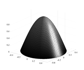
Figure 1: Elevation of the computed Poisson solution on a particular mesh.

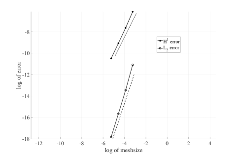
Figure 2: Convergence for the Poisson problem. Dotted line has inclination $2:1$, dashed line has inclination $3:1$.

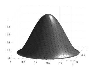
Figure 3: Elevation of the computed biharmonic solution on a particular mesh.

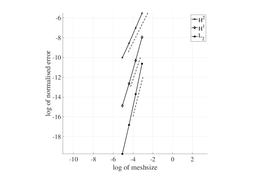
Figure 4: Convergence for the biharmonic problem. Dashed lines have inclination 2:1, 3:1, and 4:1 from top.

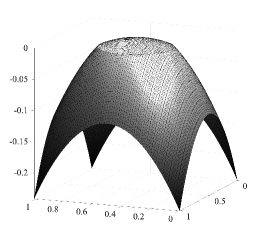
Figure 5: Elevation of the computed interface solution on a particular mesh.

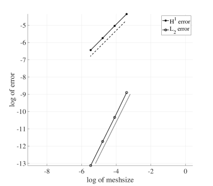
Figure 6: Convergence for the interface problem. Dashed line has inclination $1:1$ and dotted line has inclination 2:1.

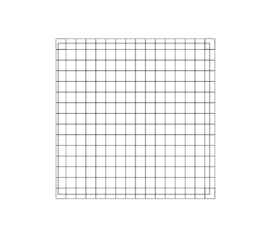
Figure 7: Mesh used for the $C^{2}$ approximation. The boundary of the domain is dotted.

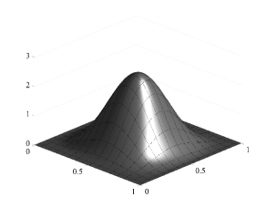
Figure 8: Elevation of computed solutions for the Poisson, biharmonic, and triharmonic problems.

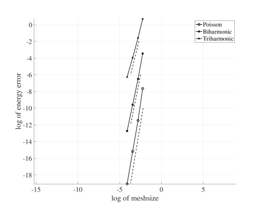
Figure 9: Energy convergence for the the Poisson, biharmonic, and triharmonic problems. Dashed lines have inclination 4:1, 5:1, and 6:1 from top.

References

• [1] S. Badia, A. F. Martin, and F. Verdugo. Mixed aggregated finite element methods for the unfitted discretization of the Stokes problem. SIAM J. Sci. Comput., 40(6):B1541–B1576, 2018.
• [2] S. Badia, F. Verdugo, and A. F. Martín. The aggregated unfitted finite element method for elliptic problems. Comput. Methods Appl. Mech. Engrg., 336:533–553, 2018.
• [3] R. Becker, E. Burman, and P. Hansbo. A Nitsche extended finite element method for incompressible elasticity with discontinuous modulus of elasticity. Comput. Methods Appl. Mech. Engrg., 198(41-44):3352–3360, 2009.
• [4] S. C. Brenner and L. R. Scott. The mathematical theory of finite element methods, volume 15 of Texts in Applied Mathematics. Springer-Verlag, New York, second edition, 2002.
• [5] E. Burman. Ghost penalty. C. R. Math. Acad. Sci. Paris, 348(21-22):1217–1220, 2010.
• [6] E. Burman, S. Claus, P. Hansbo, M. G. Larson, and A. Massing. CutFEM: discretizing geometry and partial differential equations. Internat. J. Numer. Methods Engrg., 104(7):472–501, 2015.
• [7] E. Burman and A. Ern. An unfitted hybrid high-order method for elliptic interface problems. SIAM J. Numer. Anal., 56(3):1525–1546, 2018.
• [8] E. Burman and P. Hansbo. Fictitious domain finite element methods using cut elements: II. A stabilized Nitsche method. Appl. Numer. Math., 62(4):328–341, 2012.
• [9] E. Burman and P. Hansbo. Fictitious domain methods using cut elements: III. A stabilized Nitsche method for Stokes’ problem. ESAIM Math. Model. Numer. Anal., 48(3):859–874, 2014.
• [10] E. Burman, P. Hansbo, and M. G. Larson. A cut finite element method with boundary value correction. Math. Comp., 87(310):633–657, 2018.
• [11] E. Burman, P. Hansbo, and M. G. Larson. Cut Bogner-Fox-Schmit elements for plates. Adv. Model. and Simul. in Eng. Sci., 7:27, 2020.
• [12] E. Burman, P. Hansbo, and M. G. Larson. Explicit time stepping for the wave equation using cutfem with discrete extension. Technical report, arXiv, 2020.
• [13] P. Clément. Approximation by finite element functions using local regularization. Rev. Française Automat. Informat. Recherche Opérationnelle Sér., 9(R-2):77–84, 1975.
• [14] A. Embar, J. Dolbow, and I. Harari. Imposing Dirichlet boundary conditions with Nitsche’s method and spline-based finite elements. Internat. J. Numer. Methods Engrg., 83(7):877–898, 2010.
• [15] P. Grisvard. Elliptic problems in nonsmooth domains, volume 69 of Classics in Applied Mathematics. Society for Industrial and Applied Mathematics (SIAM), Philadelphia, PA, 2011. Reprint of the 1985 original [ MR0775683], With a foreword by Susanne C. Brenner.
• [16] A. Hansbo and P. Hansbo. An unfitted finite element method, based on Nitsche’s method, for elliptic interface problems. Comput. Methods Appl. Mech. Engrg., 191(47-48):5537–5552, 2002.
• [17] A. Hansbo and P. Hansbo. A finite element method for the simulation of strong and weak discontinuities in solid mechanics. Comput. Methods Appl. Mech. Engrg., 193(33-35):3523–3540, 2004.
• [18] A. Hansbo, P. Hansbo, and M. G. Larson. A finite element method on composite grids based on Nitsche’s method. ESAIM: Math. Model. Numer. Anal., 37(3):495–514, 2003.
• [19] P. Hansbo, M. G. Larson, and S. Zahedi. A cut finite element method for a Stokes interface problem. Appl. Numer. Math., 85:90–114, 2014.
• [20] I. Harari and E. Shavelzon. Embedded kinematic boundary conditions for thin plate bending by Nitsche’s approach. Internat. J. Numer. Methods Engrg., 92(1):99–114, 2012.
• [21] P. Huang, H. Wu, and Y. Xiao. An unfitted interface penalty finite element method for elliptic interface problems. Comput. Methods Appl. Mech. Engrg., 323:439–460, 2017.
• [22] A. Johansson and M. G. Larson. A high order discontinuous Galerkin Nitsche method for elliptic problems with fictitious boundary. Numer. Math., 123(4):607–628, 2013.
• [23] J.-L. Lions and E. Magenes. Non-homogeneous boundary value problems and applications. Vol. I. Springer-Verlag, New York-Heidelberg, 1972. Translated from the French by P. Kenneth, Die Grundlehren der mathematischen Wissenschaften, Band 181.
• [24] A. Massing, M. G. Larson, A. Logg, and M. E. Rognes. A stabilized Nitsche overlapping mesh method for the Stokes problem. Numer. Math., 128(1):73–101, 2014.
• [25] L. R. Scott and S. Zhang. Finite element interpolation of nonsmooth functions satisfying boundary conditions. Math. Comp., 54(190):483–493, 1990.
• [26] E. M. Stein. Singular integrals and differentiability properties of functions. Princeton Mathematical Series, No. 30. Princeton University Press, Princeton, N.J., 1970.
• [27] V. Thomée. Galerkin finite element methods for parabolic problems, volume 25 of Springer Series in Computational Mathematics. Springer-Verlag, Berlin, second edition, 2006.
Refer to caption