Deep One-Class Classification via Interpolated Gaussian Descriptor

Abstract

One-class classification (OCC) aims to learn an effective data description to enclose all normal training samples and detect anomalies based on the deviation from the data description. Current state-of-the-art OCC models learn a compact normality description by hyper-sphere minimisation, but they often suffer from overfitting the training data, especially when the training set is small or contaminated with anomalous samples. To address this issue, we introduce the interpolated Gaussian descriptor (IGD) method, a novel OCC model that learns a one-class Gaussian anomaly classifier trained with adversarially interpolated training samples. The Gaussian anomaly classifier differentiates the training samples based on their distance to the Gaussian centre and the standard deviation of these distances, offering the model a discriminability w.r.t. the given samples during training. The adversarial interpolation is enforced to consistently learn a smooth Gaussian descriptor, even when the training data is small or contaminated with anomalous samples. This enables our model to learn the data description based on the representative normal samples rather than fringe or anomalous samples, resulting in significantly improved normality description. In extensive experiments on diverse popular benchmarks, including MNIST, Fashion MNIST, CIFAR10, MVTec AD and two medical datasets, IGD achieves better detection accuracy than current state-of-the-art models. IGD also shows better robustness in problems with small or contaminated training sets.

Introduction

Anomaly detection and segmentation are critical tasks in many real-world applications, such as the identification of defects on industry objects (Bergmann et al. 2019) or abnormalities from medical images (Schlegl et al. 2017, 2019). Given that most of the training sets available for this task contain only normal images, existing methods are typically formulated as one-class classifiers (OCC) (Venkataramanan et al. 2019; Ruff et al. 2018). OCCs aim to first learn a data description of normal samples in the training set and then use a criterion (e.g., distance to the one-class centre (Ruff et al. 2018)) to detect and localise anomalies in test samples.

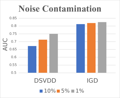
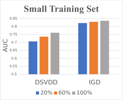
Figure 1: Mean testing AUC of DSVDD (Ruff et al. 2018), and our proposed IGD trained with the CIFAR10 training set contaminated with 1%, 5% and 10% of anomalous samples (left), and small training sets, consisting of 20%, 60%, and 100% of the CIFAR10 training set (right).

State-of-the-art (SOTA) OCC models are trained by minimising the radius of a hyper-sphere to enclose all training samples in the representation space (Ruff et al. 2018; Perera and Patel 2019; Ruff et al. 2020). To avoid catastrophic collapse, where all training samples are projected to a single point in the representation space, these OCC models fix the hyper-sphere centre and remove the bias terms from the model. Even though these SOTA OCC models show accurate anomaly detection results in several benchmarks, they can overfit the training data, particularly when the training set is small or contaminated with anomalous samples, as shown by the results of DSVDD (Ruff et al. 2018) in Fig. 1.

In this paper, we introduce the interpolated Gaussian descriptor (IGD) method to address the overfitting issue presented in SOTA OCC models. IGD is based on a one-class Gaussian anomaly classifier modelled with adversarially interpolated training samples. The classifier is trained to build a normality description to discriminate training samples based on their distance to the Gaussian centre and the standard deviation of these distances. The smoothness of the normality description is enforced by the adversarial interpolation of the training samples that constrains the training of IGD to be based on representative normal samples rather than fringe or anomalous samples. This allows the normality description of IGD to be more robust than the SOTA OCC models, particularly when the training set is small or contaminated with anomalous samples, as shown in Fig. 1 and t-SNE results in appendix.

In summary, our paper makes the following contributions:

• One novel OCC model that targets the learning of an effective normality description based on representative normal samples rather than fringe or anomalous samples, resulting in an improved anomaly classifier, compared with the SOTA;

• One new OCC optimisation approach based on a theoretically sound derivation of the expectation-maximisation (EM) algorithm that optimises a Gaussian anomaly classifier constrained by adversarially interpolated training samples and multi-scale structural and non-structural image reconstruction to enforce a smooth normality description; and

• One new OCC benchmark to assess the robustness of anomaly detectors to training sets that are small or contaminated with anomalous samples.

Extensive empirical results on six popular anomaly detection benchmarks for semantic anomaly detection, industrial defect detection, and malignant lesion detection show that our model IGD can generalise well across these diverse application domains and perform consistently better than current SOTA detectors. We also show that IGD is more robust than current OCC approaches when dealing with small and contaminated training sets.

Related Work

Unsupervised anomaly detection (UAD) is generally solved with OCCs (Li et al. 2021; Tian et al. 2021d, 2020, c; Ruff et al. 2018; Bergmann et al. 2020; Perera, Nallapati, and Xiang 2019; Salehi et al. 2021; Wang et al. 2021; Tian et al. 2021a; Bergman and Hoshen 2020; Golan and El-Yaniv 2018; Defard et al. 2021; Zavrtanik et al. 2021; Wang et al. 2016). A representative OCC model is DSVDD (Ruff et al. 2018), which forces normal image features to be inside a hyper-sphere with a pre-defined centre and a radius that is minimised to include all training images. Then, test images that fall inside the hyper-sphere are classified as normal, and the ones outside are anomalous. Although powerful, the hard boundary of SVDD can cause the model to overfit the training data – this problem was tackled with a soft-boundary SVDD (Ruff et al. 2018), but it can still overfit given that it lacks enough generalisation constraints. OCC methods can also rely on generative models, such as generative adversarial network (GAN) or Auto-encoder (AE). In (Perera, Nallapati, and Xiang 2019), a GAN is trained to produce normal samples, and its discriminator is used to detect anomalies, but the complex training process of GANs represents a disadvantage of this approach. An AE (Ionescu et al. 2019; Gong et al. 2019; Nguyen and Meunier 2019; Sabokrou et al. 2017, 2018; Venkataramanan et al. 2019) is trained to reconstruct normal data, and the anomaly score is defined as the reconstruction error between the input and reconstructed images. AE approaches depend on the MSE reconstruction loss, which does not work well for structural anomalies. Alternatively, single-scale SSIM loss (Bergmann et al. 2018) tends to work well for structural anomalies of a specific size, but it may work poorly for non-structural anomalies and structural anomalies outside that specific size. A more detailed review of these methods can be found in (Pang et al. 2021).

An important aspect of current UAD approaches is their dependence on pre-trained models to produce SOTA results. UAD models can be pre-trained on ImageNet (Venkataramanan et al. 2019; Bergmann et al. 2020) or self-supervised tasks (Golan and El-Yaniv 2018; Bergman and Hoshen 2020). To allow a fair comparison with current UAD methods, we pre-train IGD with self-supervision and ImageNet.

Unsupervised anomaly localisation targets the segmentation of anomalous image pixels or patches, containing, for example, lesions in medical images (Li et al. 2019a), defects in industry images (Bergmann et al. 2019, 2020), or road anomalies in traffic images (Pathak, Sharang, and Mukerjee 2015; Tian et al. 2021b). The main idea explored is based on extending the image based OCC to a pixel-based OCC, where testing produces a pixel-wise anomaly score map (Baur et al. 2018; Bergmann et al. 2018). In general, methods that can localise anomalies (Venkataramanan et al. 2019; Bergmann et al. 2020) are tuned to particular anomaly sizes and structure, which can cause then to miss anomalies outside that range of sizes and structure. To avoid this issue, we design IGD to detect multi-scale structural and non-structural anomalies to improve the anomaly localisation accuracy.

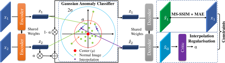
Figure 2: Our IGD consists of an encoder that transforms image $\mathbf{x}$ into representation $\mathbf{z}$, a decoder to reconstruct the image (trained with MS-SSIM and MAE losses), a Gaussian anomaly classifier trained to push the normal image representation close to the centre of the estimated normal image distribution (denoted by a Gaussian with mean $\mu$ and standard deviation $\sigma$), and a critic module that constrains the likelihood maximisation by predicting the interpolation coefficient $\alpha$ that produces a convex combination of training sample representations. Note that critic is a module similar to a GAN discriminator.

Method

We denote the training set containing only normal samples by $\mathcal{D}=\{\mathbf{x}_{i}\}_{i=1}^{|\mathcal{D}|}$, where $\mathbf{x}\in\mathcal{X}\subset\mathbb{R}^{W\times H\times 3}$ represents an RGB image of width $W$ and height $H$ and sampled from the distribution of normal images as in $\mathbf{x}\sim\mathcal{P}_{\mathcal{X}}$. The testing set contains normal and anomalous images, where anomalous images can have segmentation map annotations. This testing set is defined by $\mathcal{T}=\{(\mathbf{x}_{i},y_{i},\mathbf{b}^{({y_{i}})}_{i}\}_{i=1}^{|\mathcal{T}|}$, where $y_{i}\in\mathcal{Y}=\{0,1\}$ ($0$ denotes a normal and $1$ denotes an anomalous image), the segmentation map with the anomaly is denoted by $\mathbf{b}^{({y_{i}})}_{i}\in\{0,1\}^{W\times H}$ (i.e., a pixel-wise anomaly map for image $\mathbf{x}_{i}$) if $y_{i}=1$, and $\mathbf{b}^{({y_{i}})}_{i}=0^{W\times H}$ if $y_{i}=0$.

Interpolated Gaussian Descriptor (IGD)

As depicted in Fig. 2, the IGD model is represented by the general classifier $p_{\theta}(y=0|\mathbf{x},\mathcal{P}_{\mathcal{X}})$ that consists of an encoder $\mathbf{z}=f_{\psi}(\mathbf{x})$ that transforms a training sample from the image space $\mathcal{X}$ to a representation space $\mathcal{Z}\in\mathbb{R}^{Z}$, a Gaussian anomaly classifier $p_{\theta}(y=0|\omega,\mathbf{x})\in[0,1]$ that takes the normal image distribution parameter $\omega$ and image $\mathbf{x}$ to estimate the probability that it is normal, a decoder $\hat{\mathbf{x}}=g_{\phi}(\mathbf{z})$ that reconstructs an image from the representation space, and a critic module $\alpha=d_{\eta}(g_{\phi}(\alpha\mathbf{z}_{1}+(1-\alpha)\mathbf{z}_{2}))$ that predicts the interpolation constraint parameter $\alpha\in[0,1]$, with $\mathbf{z}_{1},\mathbf{z}_{2}$ obtained from the encoder $f_{\psi}(.)$. The IGD parameter $\theta\in\Theta$ represents all module parameters $\{\psi,\phi,\eta\}$ and is estimated with maximum likelihood estimation (MLE):

$$\theta^{*}=\arg\max_{\theta}\frac{1}{|\mathcal{D}|}\sum_{\mathbf{x}_{i}\in\mathcal{D}}\log p_{\theta}(y_{i}=0|\mathbf{x}_{i},\mathcal{P}_{\mathcal{X}}).$$ (1)

We train the one-class classifier in (1) using an EM optimisation (Dempster and Others 1977), where the mean and standard deviation of the normal image distribution are estimated during the E-step, instead of being explicitly optimised (Ruff et al. 2018), reducing the risk of overfitting. To encourage the M-step to learn an effective normality description (such that the optimisation is robust to small and contaminated training sets), we add an adversarial interpolation constraint to enforce linear combinations of normal image representations to belong to the normal distribution. We further increase the robustness of IGD to overfitting by constraining the optimisation of the M-step to enforce accurate image reconstruction from its representation. Below, we provide more details about the training process.

To formulate the EM optimisation, we re-write the log-likelihood in (1) as

$$\begin{split}\log p_{\theta}&(y_{i}=0|\mathbf{x}_{i},\mathcal{P}_{\mathcal{X}})\\ &=\ell_{ELBO}(q,\theta)+KL[q(\omega)||p_{\theta}(\omega|\mathcal{P}_{\mathcal{X}})].\end{split}$$ (2)

with $\omega\in\mathcal{W}\subset\mathbb{R}^{Z}\times\mathbb{R}$ denoting the latent variables (mean and standard deviation) that describe the distribution of normal image representations (defined in more detail below). In (2), we remove the conditional dependence of $p_{\theta}(\omega|\mathcal{P}_{\mathcal{X}})$ on $y_{i}=0$ and $\mathbf{x}_{i}$ because $\omega$ is a variable for the whole training distribution defined as

$$p_{\theta}(\omega|\mathcal{P}_{\mathcal{X}})=\delta_{a}(\|\omega(1)-\mu_{x}\|_{2})\delta_{a}(\omega(2)-\sigma_{x}),$$ (3)

where $\delta_{a}(b)=\frac{1}{|a|\sqrt{\pi}}\exp{-(b/a)^{2}}$ ($a\to 0$ approximates a Dirac delta function, and $a\to\infty$ approximates a uniform function), $\mu_{x}=\mathbb{E}_{\mathbf{x}\sim\mathcal{P}_{\mathcal{X}}}[f_{\psi}(\mathbf{x})]$ and $\sigma^{2}_{x}=\mathbb{E}_{\mathbf{x}\sim\mathcal{P}_{\mathcal{X}}}[\|f_{\psi}(\mathbf{x})-\mu_{x}\|_{2}^{2}]$, with $f_{\psi}(.)$ representing the encoder; and in (2), we also have

$$\begin{split}\ell_{ELBO}&(q,\theta)=\\ &\mathbb{E}_{q(\omega)}[\log p_{\theta}(y_{i}=0,\omega|\mathbf{x}_{i},\mathcal{P}_{\mathcal{X}})]-\mathbb{E}_{q(\omega)}[\log q(\omega)],\end{split}$$ (4)

where $KL[\cdot]$ denotes the Kullback-Leibler divergence, and $q(\omega)$ represents the variational distribution that approximates $p_{\theta}(\omega|\mathcal{P}_{\mathcal{X}})$, defined in (3).

The E-step of the EM optimisation zeroes the KL divergence in (2) by setting $q(\omega)=p_{\theta^{old}}(\omega|\mathcal{P}_{\mathcal{X}})$, where $\theta^{old}$ represents the previous EM iteration parameter value. In practice, the E-step sets $\omega(1)$ to $\mu_{x}$ and $\omega(2)$ to $\sigma_{x}$, defined in (3). Next, the M-step maximises $\ell_{ELBO}$ in (4), with:

$$\begin{split}\theta^{\star}=\arg\max_{\theta}\frac{1}{|\mathcal{D}|}\sum_{\mathbf{x}_{i}\in\mathcal{D}}\Big{(}\mathbb{E}_{q(\omega)}[&\log p_{\theta}(y_{i}=0|\omega,\mathbf{x}_{i})\\ &+\log p_{\theta}(\omega|\mathcal{P}_{\mathcal{X}})\big{]}\Big{)},\end{split}$$ (5)

where $\mathbb{E}_{q(\omega)}[\log(q(\omega))]$ is removed from $\ell_{ELBO}$ because it depends only on the previous iteration parameter $\theta^{old}$, $q(\omega)$ is defined in the E-step above, and the conditional dependence of $p_{\theta}(y=0|\omega,\mathbf{x}_{i})$ on $\mathcal{P}_{\mathcal{X}}$ is removed because the information from that distribution is summarised in $\theta$. Therefore, (5) has two components: 1) the classification term represented by the Gaussian anomaly classifier $p_{\theta}(y=0|\omega,\mathbf{x}_{i})=\exp\left(-\frac{\|f_{\psi}(\mathbf{x})-\omega(1)\|_{2}^{2}}{\omega(2)^{2}}\right)$, with mean $\omega(1)$ and standard deviation $\omega(2)$; and 2) $p_{\theta}(\omega|\mathcal{P}_{\mathcal{X}})$ defined in (3), which approximates a uniform distribution to prevent the confirmation bias of the estimated $\mu_{x}$ and $\sigma_{x}$ from (3). To promote an effective normality description of IGD, we constrain the M-step (5) as follows:

$$\max_{\theta} \frac{1}{|\mathcal{D}|}\sum_{\mathbf{x}_{i}\in\mathcal{D}}\mathbb{E}_{q(\omega)}[\log(p_{\theta}(y=0|\omega,\mathbf{x}_{i}))]$$ (6)

s.t. $$\ell_{d}(\mathbf{x}_{i},\theta)=0,\forall\mathbf{x}_{i}\in\mathcal{D},$$

$$\ell_{f,g}(\mathbf{x}_{i},\theta)=0,\forall\mathbf{x}_{i}\in\mathcal{D},$$

where $\ell_{d}(.)$ is a constraint, defined in (10), to enforce the adversarial linear interpolation of normal image representations to belong to the normal representation distribution, and $\ell_{f,g}(.)$ is a constraint, defined in (11), to enforce accurate structural and non-structural multi-scale image reconstruction. Note that the maximisation in (6) constrains the optimisation in (5), which means that we are maximising a lower bound to the original M-step. Using Lagrange multipliers, the optimisation in (6) is reformulated to minimise the following loss function:

$$\ell(\theta,\omega,\mathcal{D})=\frac{1}{|\mathcal{D}|}\sum_{i=1}^{|\mathcal{D}|}\ell_{h}(\mathbf{x}_{i},\omega,\theta)+\lambda_{1}\ell_{d}(\mathbf{x}_{i},\theta)+\lambda_{2}\ell_{f,g}(\mathbf{x}_{i},\theta),$$ (7)

where

$$\ell_{h}(\mathbf{x},\omega,\theta)=1-p_{\theta}(y=0|\omega,\mathbf{x})=p_{\theta}(y=1|\omega,\mathbf{x}),$$ (8)

with $p_{\theta}(y=0|\omega,\mathbf{x})$ defined in (5), and $\lambda_{1},\lambda_{2}$ denoting the Lagrange multipliers. The interpolation constrain $\ell_{d}(.)$ in (6) and (7) regularises the training by linearly interpolating the representations from training images, and estimating the interpolation coefficient with the critic network (Berthelot et al. 2018). This interpolation constrains the normal image distribution denser in the representation space, reducing the likelihood that anomalous representations may land in the same region of the representation space occupied by normal samples. Unlike Mix-up (Zhang et al. 2017), our interpolation constraint is a self-supervised method that does not rely on data augmentation on the input space and does not interpolate training labels, making it more adequate for our problem because it enforces a compact and dense distribution of normal samples to be estimated for the Gaussian anomaly classifier. The critic network is represented by

$$\hat{\alpha}=d_{\eta}\left(\hat{\mathbf{x}}_{\alpha}\right),$$ (9)

where $\hat{\mathbf{x}}_{\alpha}=g_{\phi}\left(\alpha\mathbf{z}_{1}+(1-\alpha)\mathbf{z}_{2}\right)$ represents the reconstruction of the interpolation of $\mathbf{z}_{1}=f_{\psi}(\mathbf{x}_{1})$ and $\mathbf{z}_{2}=f_{\psi}(\mathbf{x}_{2})$ (with $\alpha\sim\mathcal{U}(0,0.5)$, $\mathbf{x}_{1},\mathbf{x}_{2}\in\mathcal{D}$, $\mathbf{x}_{1}\neq\mathbf{x}_{2}$, and $\mathcal{U}$ denoting a uniform distribution ) (Berthelot et al. 2018), and $g_{\phi}(.)$ denotes the decoder. The goal of the critic network $d_{\eta}(.)$ is to predict the interpolation coefficient $\alpha$. The critic network in (9) is similar to the discriminator in GAN (Goodfellow et al. 2014), and relies on the following adversarial loss to be optimised (Berthelot et al. 2018)

$$\ell_{d}(\mathbf{x},\theta)=\|d_{\eta}(\hat{\mathbf{x}}_{\alpha})-\alpha\|_{2}^{2}+\|d_{\eta}(\hat{\mathbf{x}}_{\zeta})\|_{2}^{2},$$ (10)

where $\hat{\mathbf{x}}_{\alpha}$ is defined in (9), and $\hat{\mathbf{x}}_{\zeta}=\zeta\mathbf{x}+(1-\zeta)\hat{\mathbf{x}}$, with $\zeta\sim\mathcal{U}(0,1)$ and $\hat{\mathbf{x}}$ denoting a reconstruction of $\mathbf{x}$ by the auto-encoder. The first term of (10) minimises the critic’s prediction error for $\alpha$ and the second term regularises the training to ensure that the critic predicts $\hat{\alpha}=0$ when the original image is interpolated with its own reconstruction in the image space $\mathcal{X}$.

The image reconstruction constrain $\ell_{f,g}(.)$ in (6) and (7) is defined as

$$\ell_{f,g}(\mathbf{x},\theta)=\ell_{r}(\mathbf{x},\hat{\mathbf{x}},\theta)+\lambda_{3}\|d_{\eta}(\hat{\mathbf{x}}_{\alpha})\|_{2}^{2},$$ (11)

where $\hat{\mathbf{x}}$ is a reconstruction of $\mathbf{x}$ by the auto-encoder, with the image reconstruction loss $\ell_{r}(.)$ to be defined below in (12), and $\lambda_{3}$ is a hyperparameter to weight the regularisation term. This regularisation fools the critic to output $\hat{\alpha}=0$ for interpolated embeddings, independently of $\alpha$, following standard adversarial training (Goodfellow et al. 2014). In (11), we also have

$$\begin{split}\ell_{r}&(\mathbf{x},\hat{\mathbf{x}},\theta)=\\ &\sum_{\omega\in\Omega}\rho|\mathbf{x}({\omega})-\hat{\mathbf{x}}({\omega})|+(1-\rho)\Big{(}1-m\big{(}\mathbf{x}({\omega}),\hat{\mathbf{x}}({\omega})\big{)}\Big{)},\end{split}$$ (12)

with $\Omega$ denoting the image lattice, $\rho\in[0,1]$, $|\mathbf{x}({\omega})-\hat{\mathbf{x}}({\omega})|$ representing the MAE loss, and $m(\mathbf{x}({\omega}),\hat{\mathbf{x}}({\omega}))\in[0,1]$ being the MS-SSIM score (Wang, Simoncelli, and Bovik 2003), with larger values indicating higher similarity between patches $\omega\in\Omega$ of the original and reconstructed images. Please see details on how to compute the MS-SSIM score in the Supp. Material.

The loss in (7) is used to train two models (see ’Global and Local IGD Models’ section in the Supp. Material). A global model that works on the whole image $\mathbf{x}$, and a local model that works on image patches $\mathbf{x}^{(L)}({\omega})\in\mathcal{X}^{(L)}\subset\mathbb{R}^{W^{(L)}\times H^{(L)}\times 3}$, with $W^{(L)}<W$ and $H^{(L)}<H$, centred at pixel $\omega\in\Omega$ ($\Omega$ is the image lattice). During inference, the results from the global and local models are combined to produce multi-scale anomaly detection and localisation. Please see the Supp. Material for a visual example of the results produced by the global and local models.

Theoretical Guarantees

IGD maximises a constrained $\ell_{ELBO}(q,\theta)$ in (6) rather than maximising $p_{\theta}(y=0|\mathbf{x},\mathcal{P}_{\mathcal{X}})$ in (1). Using Theorem 1 in (Dempster and Others 1977), Lemma .3 demonstrates the correctness of IGD, where an increase to the constrained $\ell_{ELBO}(q,\theta)$ implies an increase to $p_{\theta}(y=0|\mathbf{x},\mathcal{P}_{\mathcal{X}})$. Using Theorem 2 in (Dempster and Others 1977), Lemma .4 proves the convergence conditions of IGD.

Lemma 0.1.

Assuming that the maximisation of the constrained $\ell_{ELBO}$ in (6) produces $\theta$ that makes
$\mathbb{E}_{q(\omega)}[\log p_{\theta}(y=0,\omega|\mathbf{x},\mathcal{P}_{\mathcal{X}})]\geq\mathbb{E}_{q(\omega)}[\log p_{\theta^{old}}(y=0,\omega|\mathbf{x},\mathcal{P}_{\mathcal{X}})]$,
we have that $\left(\log p_{\theta}(y=0|\mathbf{x},\mathcal{P}_{\mathcal{X}})-\log p_{\theta^{old}}(y=0|\mathbf{x},\mathcal{P}_{\mathcal{X}})\right)$ is lower bounded by
$\left(\mathbb{E}_{q(\omega)}[\log p_{\theta}(y=0,\omega|\mathbf{x},\mathcal{P}_{\mathcal{X}})]-\mathbb{E}_{q(\omega)}[\log p_{\theta^{old}}(y=0,\omega|\mathbf{x},\mathcal{P}_{\mathcal{X}})]\right)\geq 0$,
with $q(\omega)=p_{\theta^{old}}(\omega|\mathcal{P}_{\mathcal{X}})$.

Proof.

Please see proof in Supp. Material. ∎

Lemma 0.2.

Assume that $\{\theta^{(e)}\}_{e=1}^{+\infty}$ denotes the sequence of trained model parameters from the constrained optimisation of $\ell_{ELBO}$ in (6) such that: 1) the sequence $\{\log p_{\theta^{(e)}}(y=0|\mathbf{x},\mathcal{P}_{\mathcal{X}})\}_{e=1}^{+\infty}$ is bounded above, and 2) $\left(\mathbb{E}_{q(\omega)}[\log p_{\theta^{(e+1)}}(y=0,\omega|\mathbf{x},\mathcal{P}_{\mathcal{X}})]-\mathbb{E}_{q(\omega)}[\log p_{\theta^{(e)}}(y=0,\omega|\mathbf{x},\mathcal{P}_{\mathcal{X}})]\right)\geq$
$\xi\left(\theta^{(e+1)}-\theta^{(e)}\right)^{\top}\left(\theta^{(e+1)}-\theta^{(e)}\right)$ , for $\xi>0$ and all $e\geq 1$, and $q(\omega)=p_{\theta^{(e)}}(\omega|\mathcal{P}_{\mathcal{X}})$. Then $\{\theta^{(e)}\}_{e=1}^{+\infty}$ converges to some $\theta^{\star}\in\Theta$.

Proof.

Please see proof in Supp. Material. ∎

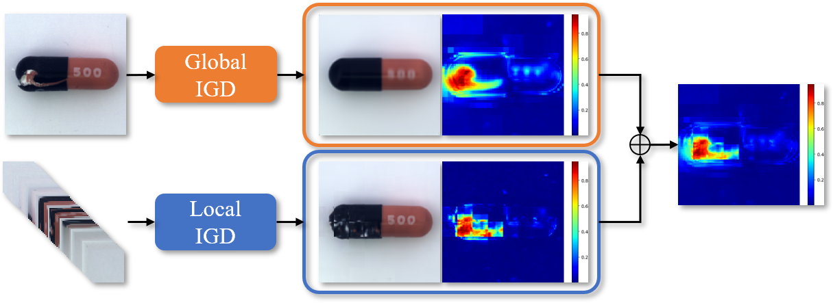
Figure 3: Example of the multi-scale structural and non-structural anomaly localisation result for an MVTec AD (Bergmann et al. 2019) image, using both the local and global IGD models. The global model tends to produce smooth results but with some mistakes, while the local model produces jagged results, but without the global mistakes, so by combining the two results, we obtain a smooth and correct anomaly heatmap.

Training and Inference

The global and local IGD models are trained separately (see Fig. S1), following the EM optimisation, where the E-step estimates the the latent variable $\omega$ in (3), and the M-step minimises the loss in (7) to obtain $\theta^{\star}$.

During inference, anomaly detection is performed by combining the global and local IGD anomaly scores for a testing image $\mathbf{x}$ as in:

$$s(\mathbf{x})=s^{(G)}(\mathbf{x})+s^{(L)}(\mathbf{x}).$$ (13)

The global score in (13) is defined as

$$s^{(G)}(\mathbf{x})=\ell^{(G)}_{r}(\mathbf{x},\hat{\mathbf{x}},\theta^{*})+\ell^{(G)}_{h}(\mathbf{x},\theta^{*}),$$ (14)

where $\ell^{(G)}_{r}(.)$ denotes the reconstruction loss from (12) and $\ell^{(G)}_{h}(.)$ denotes the Gaussian anomaly classification loss from (8) (both computed with the global IGD model using the whole images), and $\hat{\mathbf{x}}$ is the reconstruction of $\mathbf{x}$ produced by the auto-encoder. The local score in (13) is defined as

$$\begin{split}s^{(L)}(\mathbf{x})=\max_{\omega\in\Omega}\Big{(}&\ell^{(L)}_{r}\big{(}\mathbf{x}^{(L)}({\omega}),\hat{\mathbf{x}}^{(L)}({\omega}),\theta^{*}\big{)}+\\ &\ell^{(L)}_{h}\big{(}\mathbf{x}^{(L)}({\omega}),\theta^{*}\big{)}\Big{)},\end{split}$$ (15)

where $\ell^{(L)}_{r}(.)$ and $\ell^{(L)}_{h}(.)$ are the reconstruction and Gaussian anomaly classification losses computed from the local model, with $\mathbf{x}^{(L)}({\omega})$ denoting an image patch of size $W^{(L)}\times H^{(L)}\times 3$ at pixel $\omega\in\Omega$. The use of max pooling of the local scores in (15) facilitates detection of images that contain anomalies covering a small region of the image. Anomaly localisation is computed for each pixel $\omega\in\Omega$ to produce a local score

$$\begin{split}l(\mathbf{x}({\omega}))=&\ell^{(G)}_{r}\big{(}\mathbf{x}(\omega),\hat{\mathbf{x}}(\omega),\theta^{*}\big{)}+\\ &\ell^{(L)}_{r}\big{(}\mathbf{x}^{(L)}({\omega}),\hat{\mathbf{x}}^{(L)}({\omega}),\theta^{*}\big{)},\end{split}$$ (16)

with

$$\begin{split}\ell^{(G)}_{r}\big{(}\mathbf{x}(\omega),&\hat{\mathbf{x}}(\omega),\theta^{*}\big{)}=\rho\big{|}\mathbf{x}(\omega)-\hat{\mathbf{x}}(\omega)\big{|}+\\ &(1-\rho)\Big{(}1-m^{(G)}\big{(}\mathbf{x}(\omega),\hat{\mathbf{x}}(\omega)\big{)}\Big{)},\end{split}$$ (17)

where $\rho$ and $m^{(G)}(.)$ are defined in (12) and $\hat{\mathbf{x}}$ is a reconstruction of $\mathbf{x}$ produced by the global IGD model. The $\ell^{(L)}_{r}\big{(}\mathbf{x}^{(L)}({\omega}),\hat{\mathbf{x}}^{(L)}({\omega}),\theta^{*}\big{)}$ in (16) is similarly defined using the local IGD model. Thus, the anomaly localisation final map is a heatmap with high values representing regions that are likely to contain anomalies, as displayed in ’Global and Local IGD Models’ section in the Supp. Material.

Experiments

Datasets and Evaluation Metric

Datasets: We use four computer vision and two medical image datasets to evaluate our methods. The computer vision datasets are MNIST (LeCun, Cortes, and Burges 2010), Fashion MNIST (Xiao, Rasul, and Vollgraf 2017), CIFAR10 (Krizhevsky, Nair, and Hinton 2014) and MVTec AD (Bergmann et al. 2019); and the medical image datasets are Hyper-Kvasir (Borgli and et al. 2020) and LAG (Li et al. 2019b). MNIST, Fashion MNIST and CIFAR10 have been widely used as benchmarks for image anomaly detection, and we follow the same experimental protocol as described in (Ruff et al. 2018). CIFAR10 contains 60,000 images with 10 classes. MNIST and Fashion MNIST contain 70,000 images with 10 classes of handwritten digits and fashion products, respectively. MVTec AD (Bergmann et al. 2019) contains 5,354 high-resolution real-world images of 15 different industry object and textures. The normal class of MVTec AD is formed by 3,629 training and 467 testing images without defects. The anomalous class has more than 70 categories of defects (such as dents, structural fails, contamination, etc.) and contains 1,258 testing images. MVTec AD provides pixel-wise ground truth annotations for all anomalies in the testing images, allowing the evaluation of anomaly detection and localisation. We also tested our method on two publicly available medical datasets: Hyper-Kvasir (Borgli and et al. 2020) and LAG (Li et al. 2019b) for polyp and glaucoma detection, respectively. For Hyper-Kvasir, we has 1,600 normal images without polyps in the training set and 500 in the testing set; and 1,000 abnormal images containing polyps in the testing set. For LAG, we have 2,343 normal images without glaucoma in the training set; and 800 normal images and 1,711 abnormal images with glaucoma for testing.

Evaluation: For anomaly detection, we assess performance with the area under the receiver operating characteristic curve (AUC) and classification accuracy. On MNIST, Fashion MNIST and CIFAR10, we use the same protocol as other methods in Tab. 1, where training uses a single class as the normal data, with the nine remaining classes denoting as semantically anomalous samples, and inference relies on a non-augmented test image. We report the mean AUC over the 10 classes for the above three data sets. On MVTec AD (Bergmann et al. 2020; Venkataramanan et al. 2019), we evaluate anomaly detection with mean AUC and accuracy. Follow previous works (Tian et al. 2021d, a), we evaluate the methods using AUC for the Hyper-Kvasir and LAG. For anomaly localisation, we follow (Venkataramanan et al. 2019) and compute the mean pixel-level AUC between the generated heatmap and the ground truth segmentation map for each anomalous image in the testing set of MVTec AD.

Pretrain	Method	MNIST	CIFAR10	FMNIST
Scratch	DAE (Hadsell et al. 2006)	0.8766	0.5358	-
	VAE (Kingma and Welling 2013)	0.9696	0.5833	-
	KDE (Bishop 2006)	0.8140	0.6100	-
	OCSVM (Schölkopf et al. 2001)	0.9510	0.5860	-
	AnoGAN (Schlegl et al. 2017)	0.9127	0.6179	-
	DSVDD (Ruff et al. 2018)	0.9480	0.6481	-
	OCGAN (Perera, Nallapati, and Xiang 2019)	0.9750	0.6566	-
	PixelCNN (Van den Oord et al. 2016)	0.6180	0.5510	-
	CapsNetPP (Li et al. 2020)	0.9770	0.6120	0.7650
	CapsNetRE (Li et al. 2020)	0.9250	0.5310	0.6790
	ADGAN (Deecke et al. 2018)	0.9680	0.6340	-
	LSA (Abati et al. 2019)	0.9750	0.6410	0.8760
	MemAE (Gong et al. 2019)	0.9751	0.6088	-
	GradCon (Kwon et al. 2020)	0.9730	0.6640	-
	$\lambda$-VAEu (Dehaene et al. 2020)	0.9820	0.7170	0.8730
	ULSLM (Wolf et al. 2020)	0.9490	0.7360	-
	SCADN (Yan et al. 2021)	0.9771	0.6690	-
	Ours	0.9869	0.7433	0.9201
ImageNet	CAVGA-Du (Venkataramanan et al. 2019)	0.9860	0.7370	0.8850
	Student-Teacher (Bergmann et al. 2020)	0.9935	0.8196	-
	Ours	0.9927	0.8368	0.9357
SSL	Rot-Net (Golan and El-Yaniv 2018)	-	0.8160	0.9350
	Bergman and Hoshen (2020)	-	0.8820	0.9410
	Ours	-	0.9125	0.9441

Table 1: Anomaly detection: mean AUC testing results on MNIST, CIFAR10 and Fashion MNIST. The results are split into ’Scratch’ (without any pre-training), pretrained with ’ImageNet’, and self-supervised learning (’SSL’). Bold numbers represent the best result (within 0.5%) for each data set, discriminated by Scratch, SSL or ImageNet.

Implementation Details

We implement our framework using Pytorch. The model was trained with Adam optimiser using a learning rate of 0.0001, weight decay of $10^{-6}$, batch size of 64 images, 256 epochs for all dataset. We defined the representation space produced by the encoder to have $Z=128$ dimensions. Following (Godard, Mac Aodha, and Brostow 2017), we set $\rho=0.15$ to balance the contribution of MAE and MS-SSIM losses in (12) and (17). We set $\lambda_{1}=\lambda_{2}=1$ in (7) and $\lambda_{3}=0.1$ in (11), based on cross validation experiments. We use Resnet18 and its reverse architecture as the encoder and decoder for both the global and local IGD models. When computing the accuracy of anomaly detection in MVTec AD, the threshold of the anomaly detection score $s(\mathbf{x})$ in (13) (to classify an image as anomalous) is set to 0.5 (Venkataramanan et al. 2019). To enable a fair comparison between our method and previous approaches in the field (Bergmann et al. 2020; Venkataramanan et al. 2019; Bergman and Hoshen 2020; Golan and El-Yaniv 2018), we pre-train the encoders for the global and local IGD models either with self-supervised learning (SSL) (Chen et al. 2020) or ImageNet knowledge distillation (KD) (Bergmann et al. 2020; Gou et al. 2020). For this SSL pre-training, we use the SGD optimiser with a learning rate of 0.01, weight decay $10^{-1}$, batch size of 32, and 2,000 epochs. Once we obtain the pre-trained encoder with SSL, we remove the MLP layer and attach a linear layer to the backbone with fixed parameters. Note that this SSL is trained from scratch. In contrast to the vanilla self-supervised learning (Chen et al. 2020) suggesting large batch size, we notice that a medium batch size yields significantly better performance for unsupervised anomaly detection.

For the ImageNet KD pre-training, we minimise the $\ell 2$ norm between the 512-dimensional feature vector output from encoder and an intermediate layer of the ImageNet pre-trained ResNet18 with the same 512-dimensional features. For this ImageNet KD pre-training, we use the Adam optimiser with a learning rate of 0.0001, weight decay $10^{-5}$, batch size of 64, and 50,000 iterations. Once we obtain the pre-trained encoder of KD, we fix the network parameters and attach a linear layer to reduce the dimensionality of the feature space to 128.

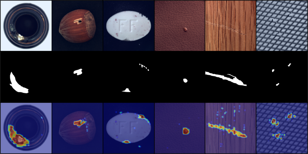
Figure 4: Qualitative results of our anomaly localisation results on the MVTec AD (red = high probability of anomaly). Top, middle and bottom rows show the testing images, ground-truth masks and predicted heatmaps, respectively. Please see additional results in the Supp. Material.

Experiments on MNIST, Fashion MNIST and CIFAR10

Table 1 compares the unsupervised anomaly detection mean AUC testing results between our method and the current SOTA on MNIST, Fashion MNIST and CIFAR10. The rows labelled as ‘Scratch’ show results of models that were not pre-trained, and the ones with ‘SSL’ display results from models using self-supervised learning method (Golan and El-Yaniv 2018; Bergman and Hoshen 2020). The ones with ‘ImageNet’ show results from models that use ImageNet KD pre-training (Venkataramanan et al. 2019; Bergmann et al. 2020). Our proposed IGD outperforms current SOTA methods for the majority of pre-training methods on all three datasets. Please see additional results in the Supp. material.

Experiments on MVTec AD

We report the results, based on SSL and ImageNet KD pre-trained models, for both anomaly detection (Tab. 2) and localisation (Tab. 3) on MVTec AD, which contains real-world images of industry objects and textures containing different types of anomalies. Following (Venkataramanan et al. 2019) the score threshold is set to 0.5 for calculating the mean accuracy of anomaly detection. For anomaly detection, our method produces the best accuracy (at least 2% better than previous SOTA) and AUC (at least 5% better than previous SOTA) results independently of the pre-training technique. For anomaly localisation, we compare our method and the SOTA using the mean pixel-level AUC of all anomalous images in the testing set of MVTec AD. Notice that our method with ImageNet and SSL pre-training are better than the previous SOTA CAVGA-R_u (Venkataramanan et al. 2019) by 2% and 4%, respectively. Fig. 4 shows anomaly localisation results on MVTec AD images, where red regions in the heatmap indicate higher anomaly probability. From this results, we can see that our approach can localise anomalous regions of different sizes and structures from different object categories. Please see additional results in the Supp. material.

Metric	Method	Mean
Accuracy	AVID (Sabokrou et al. 2018)	0.730
	AESSIM (Bergmann et al. 2018)	0.630
	DAE (Hadsell et al. 2006)	0.710
	AnoGAN (Schlegl et al. 2017)	0.550
	$\lambda$-VAEu (Dehaene et al. 2020)	0.770
	LSA (Abati et al. 2019)	0.730
	CAVGA-Du (Venkataramanan et al. 2019)	0.780
	CAVGA-Ru (Venkataramanan et al. 2019)	0.820
	Ours - ImageNet	0.840
	Ours - SSL	0.850
AUC	AnoGAN (Schlegl et al. 2017)	0.503
	GANomaly (Akcay et al. 2018)	0.782
	Skip-GANomaly (Akçay et al. 2019)	0.805
	SCADN (Yan et al. 2021)	0.818
	U-Net (Ronneberger et al. 2015)	0.819
	DAGAN (Tang et al. 2020)	0.873
	Ours - ImageNet	0.926
	Ours - SSL	0.934

Table 2: Anomaly detection: mean testing accuracy and AUC on MVTec AD produced by the SOTA and our IGD.

Method	MVTec AD
DAE (Hadsell et al. 2006)	0.82
AESSIM (Bergmann et al. 2018)	0.87
AVID (Sabokrou et al. 2018)	0.78
SCADN (Yan et al. 2021)	0.75
LSA (Abati et al. 2019)	0.79
$\lambda$-VAEu (Dehaene et al. 2020)	0.86
AnoGAN (Schlegl et al. 2017)	0.74
ADVAE (Liu et al. 2020)	0.86
CAVGA-Du (Venkataramanan et al. 2019)	0.85
CAVGA-Ru (Venkataramanan et al. 2019)	0.89
Ours - ImageNet	0.91
Ours - SSL	0.93

Table 3: Anomaly localisation: mean pixel-level AUC testing results on the anomalous images of MVTec AD.

Experiments on Medical Datasets

To show that our method can generalise to other domains, we evaluate our approach on two public medical datasets - Hyper-Kvasir for polyp detection and LAG for glaucoma detection. As shown in Tab. 4, our SSL and ImageNet based results achieve the best AUC results on both datasets. Our methods surpass the recent proposed CAVGA-R_u (Venkataramanan et al. 2019) on both datasets by a minimum 0.9% and maximum 3.8%. Also, our model performs better compared to the anomaly detector specifically designed for medical data, such as f-anogan (Schlegl et al. 2019) and ADGAN (Liu et al. 2019). We show qualitative polyp segmentation results in the Supp. Material. The abnormalities in medical data (i.e., colon polyps, glaucoma) are significantly different than the popular image benchmarks and MVTec AD in terms of appearance and structural anomalies, suggesting that our model works in disparate domains. Please see more results in the Supp. material.

Methods	Hyper-Kvasir	LAG
DAE (Masci and et al. 2011)	0.705	0.651
CAM (Zhou et al. 2016)	-	0.663
GBP (Springenberg et al. 2014)	-	0.787
SmoothGrad (Smilkov et al. 2017)	-	0.795
OCGAN (Perera et al. 2019)	0.813	0.737
F-anoGAN (Schlegl et al. 2019)	0.907	0.778
ADGAN (Liu et al. 2019)	0.913	0.752
CAVGA-$R_{u}$ (Venkataramanan et al. 2019)	0.928	0.819
Ours - ImageNet	0.931	0.838
Ours - SSL	0.937	0.857

Table 4: Anomaly detection: AUC testing results on two medical datasets: Hyper-Kvasir and LAG.

Ablation Study

To investigate the effectiveness of each component of our method, we show the mean AUC results of our method with different proposed variants in Tab. 5. Note that all results are based on the initialisation of knowledge distillation from ImageNet. For standard anomaly detection settings (AUC - Full), each proposed component of our IGD improves performance by a minimum 1.7% and maximum 11.6% mean AUC. Tab. 5 also shows the effectiveness of each component when trained with small (20% of full training data) or anomaly contaminated (10% of contamination rate) training sets, where our proposed Gaussian anomaly classifier (GAC) significantly improves over the REC (i.e., MS-SSIM+MAE losses) baseline by 13% and 10.4% mean AUC. The proposed adversarial interpolation regularisation (INTER) further improves the AUC by 3.7% and 3.1%.

MSE	REC	GAC	INTER	AUC - Full	AUC - ST	AUC - AC
✓				0.615	0.552	0.565
	✓			0.731	0.655	0.677
	✓	✓		0.819	0.785	0.781
	✓	✓	✓	0.836	0.822	0.812

Table 5: Ablation study of our method on CIFAR10 using anomaly detection mean testing AUC w.r.t standard OCC setup (AUC - Full), small training set containing 20% of training data (AUC - ST), and anomaly contaminated training set with 10% contamination (i.e., 10% of the anomalous samples are removed from the testing set and inserted into the training set) (AUC - AC). MSE denotes the baseline deep autoencoder with MSE loss, REC denotes the baseline deep autoencoder with MS-SSIM + MAE losses, GAC denotes our proposed Gaussian anomaly classifier, INTER represents our interpolation regularisation. The encoder of all above methods are initialised based on the knowledge distillation from ImageNet.

Experiments on Small/Contaminated Training Sets

Dataset	Train Size	DSVDD	DSVDD+REC	IGD (Ours)
CIFAR10	20%	0.7064	0.7462	0.8219
	60%	0.7367	0.7807	0.8298
	100%	0.7612	0.7950	0.8365
MVTec	20%	0.7994	0.7291	0.9043
	60%	0.8467	0.7737	0.9246
	100%	0.8579	0.7826	0.9260

Table 6: Mean testing AUCs on CIFAR10 and MVTec with small training sets, where REC=MS-SSIM+MAE losses.

To show the improved robustness of our approach to small training sets on CIFAR10 and MVTec, we compare the performance of DSVDD, DSVDD+REC (i.e., DSVDD combined with our reconstruction loss), and our proposed IGD, using less normal data in the training sets in Tab. 6. In particular, we randomly sub-sample 20%, 60%, and 100% of the original training sets of CIFAR10 and MVTec AD, to form a smaller training set. The results indicate that IGD achieves comparable performance under significantly less training data, while the performance of DSVDD and DSVDD+REC deteriorate dramatically when the number of training samples decreases. This result shows that IGD has better robustness than DSVDD and DSVDD+REC to small training sets.

Dataset	Noise Ratio	DSVDD	DSVDD+REC	IGD (Ours)
CIFAR10	1%	0.7502	0.7694	0.8252
	5%	0.7124	0.7448	0.8193
	10%	0.6717	0.7073	0.8122
MVTec	1%	0.8523	0.7873	0.9363
	5%	0.8391	0.7733	0.9319
	10%	0.8175	0.7687	0.9363

Table 7: Mean testing AUCs on CIFAR10 and MVTec with different contamination noise rates. REC defined in Tab. 6.

To show the improved robustness of our approach contaminated training sets, in Tab. 7, we compare the performance of DSVDD, DSVDD+REC, and our IGD, using training sets corrupted with anomalous samples (this contamination facilitates overfitting). In particular, we re-organise the original training and test data of CIFAR10 and MVTec AD by randomly sampling 1%, 5% and 10% of anomalies from the test data to inject into the training data. With different rates of anomaly contamination, the maximum fluctuation of our IGD is 1.3% on CIFAR10 and 0.44% on MVTec AD. While the competing method DSVDD shows a much larger maximum fluctuation of 7.8% and 3.5% mean AUC, on CIFAR10 and MVTec AD, respectively. The results show the substantially better robustness of IGD over DSVDD and DSVDD+REC for the anomaly-contaminated training data.

Discussion

We do not compare some of the SOTA works (Reiss et al. 2021; Sohn et al. 2020; Tack et al. 2020) in Table 1, 2, and 3 due to unfair comparison. In particular, the comparison with PANDA (Reiss et al. 2021) is not fair because it uses a WideResNet50 $\times$ 2 for MVTec and ResNet152 for CIFAR, both being much larger backbones than our ResNet18. Regarding CSI (Tack et al. 2020), it has much slower inference (because of the $40\times$ data augmentation of test images) and more complex training that needs a coreset and large batch size of 512 for pre-training, which challenges its use for problems with small training sets or high-resolution images. For both CSI and DROC (Sohn et al. 2020), their gains are mostly from the SSL pre-training. To show that point for CSI, we use our training approach to fine-tune a pre-trained CSI model and obtain 94.6% AUC on CIFAR10, which is higher than CSI (94.3% AUC). Also, for the vanilla SSL pre-training reported in DROC paper, their performance reduces from 92.5% to 89.0% AUC on CIFAR10, and from 86.5% to 80.2% AUC on MVTec. Note that all above results are collected from their published papers unless stated otherwise.

Furthermore, on MVTec, our approach obtains (93.4% AUC), which is much better than CSI (63.6% AUC from Tab.2 of (Reiss and Hoshen 2021)) and PANDA (86.5%). For anomaly localisation on MVTec, our 93% AUC is better than DROC (90%) and worse than PANDA (96%). On high-resolution image datasets (e.g., Hyper-Kvasir), our approach (93.7% AUC) is better than CSI (trained by us) that reaches 91.6% AUC. Other important results shown by our paper, but missed by CSI, PANDA and DROC, are the ones with small training sets and contaminated training sets, which are new and important benchmarks for real-world industrial applications and early detection of medical diseases.

Conclusion

In this paper, we presented a new OCC model, called interpolated Gaussian descriptor (IGD), to perform unsupervised anomaly detection and segmentation. IGD learns a one-class Gaussian anomaly classifier trained with adversarially interpolated training samples to enable an effective normality description based on representative normal samples rather than fringe or anomalous samples. The optimisation of IGD is formulated as an EM algorithm, which we show to be theoretically correct and to converge to a stationary solution under certain conditions. To our knowledge, IGD is the first method that is able to achieve the best performance across diverse application datasets, including MNIST, CIFAR10, Fashion MNIST, MVTec AD, and two large scale medical datasets, in terms of anomaly detection and localisation. We also show that IGD is more robust than DSVDD and an image-reconstruction contrained DSVDD in problems with small or contaminated training sets. We plan to study the use of Gaussian anomaly classifier in the pixel-wise localisation of anomalies and to investigate new self-supervised learning approaches specifically designed for anomaly detection.

Datasets

CIFAR10 contains 60,000 images with 10 classes. MNIST and Fashion MNIST contain 70,000 images with 10 classes of handwritten digits and fashion products, respectively. MVTec AD (Bergmann et al. 2019) contains 5,354 high-resolution real-world images of 15 different industry object and textures. The normal class of MVTec AD is formed by 3,629 training and 467 testing images without defects. The anomalous class has more than 70 categories of defects (such as dents, structural fails, contamination, etc.) and contains 1,258 testing images. MVTec AD provides pixel-wise ground truth annotations for all anomalies in the testing images, allowing the evaluation of anomaly detection and localisation. Hyper-Kvasir has 1,600 normal images without polyps in the training set and 500 in the testing set; and 1,000 abnormal images containing polyps in the testing set. For LAG, we have 2,343 normal images without glaucoma in the training set; and 800 normal images and 1,711 abnormal images with glaucoma for testing.

Global and Local IGD Models

Figure S1 shows an example of a multi-scale structural and non-structural anomaly localisation result for an MVTec AD image, using both the local and global IGD models.

Figure S1: Example of the multi-scale structural and non-structural anomaly localisation result for an MVTec AD (Bergmann et al. 2019) image, using both the local and global IGD models. The global model tends to produce smooth results but with some mistakes, while the local model produces jagged results, but without the global mistakes, so by combining the two results, we obtain a smooth and correct anomaly heatmap.

Multi-scale Structure Similarity Index (MS-SSIM) Score

The MS-SSIM loss uses the MS-SSIM global score, defined as

$$\begin{split}m^{(G)}(\mathbf{x}({\omega}),&\hat{\mathbf{x}}({\omega}))=[l_{M}(\mathbf{x}({\omega}),\hat{\mathbf{x}}({\omega}))]^{\alpha_{M}}\times\\ &\prod_{m=1}^{m^{(G)}}[c_{m}(\mathbf{x}({\omega}),\hat{\mathbf{x}}({\omega}))]^{\beta_{m}}[s_{m}(\mathbf{x}({\omega}),\hat{\mathbf{x}}({\omega}))]^{\gamma_{m}},\end{split}$$ (S1)

where $\mathbf{x}({\omega})$ denotes an image patch centred at $\omega\in\Omega$ of size $11\times 11\times 3$,

$$l_{M}(\mathbf{x}({\omega}),\hat{\mathbf{x}}({\omega}))=\frac{2\mu_{\mathbf{x}({\omega})}\mu_{\hat{\mathbf{x}}({\omega})}+C_{1}}{\mu_{\mathbf{x}({\omega})}^{2}+\mu_{\hat{\mathbf{x}}({\omega})}^{2}+C_{1}},$$ (S2)

$$c_{m}(\mathbf{x}({\omega}),\hat{\mathbf{x}}({\omega}))=\frac{2\sigma_{\mathbf{x}({\omega})}\sigma_{\hat{\mathbf{x}}({\omega})}+C_{2}}{\sigma_{\mathbf{x}({\omega})}^{2}+\sigma_{\hat{\mathbf{x}}({\omega})}^{2}+C_{2}},$$ (S3)

$$s_{m}(\mathbf{x}({\omega}),\hat{\mathbf{x}}({\omega}))=\frac{\sigma_{\mathbf{x}({\omega})\hat{\mathbf{x}}({\omega})}+C_{3}}{\sigma_{\mathbf{x}({\omega})}\sigma_{\hat{\mathbf{x}}({\omega})}+C_{3}},$$ (S4)

with $C_{1},C_{2},C_{3}$ representing pre-defined constants, $\mu_{\mathbf{x}({\omega})}$ denoting the mean intensities of $\mathbf{x}({\omega})$, $\sigma^{2}_{\mathbf{x}({\omega})}$ the variance of $\mathbf{x}({\omega})$, and $\sigma_{\mathbf{x}({\omega})\hat{\mathbf{x}}({\omega})}$ the covariance of $\mathbf{x}({\omega})$ and $\hat{\mathbf{x}}({\omega})$. In (S1), $m^{(G)}=5$ denotes the number of scales, $\beta_{1}=\gamma_{1}=0.0448$, $\beta_{2}=\gamma_{2}=0.2856$, $\beta_{3}=\gamma_{3}=0.3001$, $\beta_{4}=\gamma_{4}=0.2363$, $\alpha_{5}=\beta_{5}=\gamma_{5}=0.1333$ (Wang, Simoncelli, and Bovik 2003). We follow $C_{i}=\left(K_{i}L\right)^{2}$ (for $i\in\{1,2,3\}$) according to (Wang et al. 2004) and define $L=4.7579$ as the pixel range with $K_{1}=0.01$, $K_{2}=0.03$ and $C_{3}=C_{2}/2$.

The local score $m^{(L)}(\mathbf{x}^{(L)}({\omega}),\hat{\mathbf{x}}^{(L)}({\omega}))$ is defined in the same way as in (S1), where $\mathbf{x}^{(L)}({\omega})$ is an image patch centred at $\omega\in\Omega$ of size $3\times 3\times 3$, $m^{(L)}=4$ scales with weights $\beta_{1}=\gamma_{1}=0.0516$, $\beta_{2}=\gamma_{2}=0.3295$, $\beta_{3}=\gamma_{3}=0.3463$, $\alpha_{4}=\beta_{4}=\gamma_{4}=0.2726$ modified based on the original proportion for $m^{(G)}=5$.

Implementation Details

For this SSL pre-training, we use the SGD optimiser with a learning rate of 0.01, weight decay $10^{-1}$, batch size of 32, and 2,000 epochs. Once we obtain the pre-trained encoder with SSL, we remove the MLP layer and attach a linear layer to the backbone with fixed parameters. Note that this SSL is trained from scratch. In contrast to the vanilla self-supervised learning (Chen et al. 2020) suggesting large batch size, we notice that a medium batch size yields significantly better performance for unsupervised anomaly detection.

For the ImageNet KD pre-training, we minimise the $\ell 2$ norm between the 512-dimensional feature vector output from encoder and an intermediate layer of the ImageNet pre-trained ResNet18 (He et al. 2016) with the same 512-dimensional features. For this ImageNet KD pre-training, we use the Adam optimiser with a learning rate of 0.0001, weight decay $10^{-5}$, batch size of 64, and 50,000 iterations. Once we obtain the pre-trained encoder of KD, we fix the network parameters and attach a linear layer to reduce the dimensionality of the feature space to 128.

Visualisation of the Distribution of Testing Samples

Figure S2 shows the distribution of testing samples in the representation space, using the t-SNE visualisation, for DSVDD (Ruff et al. 2018), Gaussian anomaly classifier (GAC), and our IGD. Notice that the normal samples seem to be more compactly represented with fewer anomalous samples appearing inside the normal cluster. This suggests that IGD has a superior normality description, compared with DSVDD and GAC.

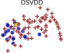
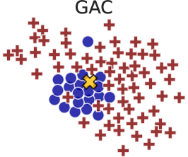
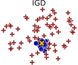
Figure S2: t-sne visualisation from MVTec (class bottle).

Metric	Method	Bottle	Hazelnut	Capsule	Metal Nut	Leather	Pill	Wood	Carpet	Tile	Grid	Cable	Transistor	Toothbrush	Screw	Zipper	Mean
Accuracy	AVID (Sabokrou et al. 2018)	0.85	0.86	0.85	0.63	0.58	0.86	0.83	0.70	0.66	0.59	0.64	0.58	0.73	0.66	0.84	0.73
	AESSIM (Bergmann et al. 2018)	0.88	0.54	0.61	0.54	0.46	0.60	0.83	0.67	0.52	0.69	0.61	0.52	0.74	0.51	0.80	0.63
	DAE (Hadsell et al. 2006)	0.80	0.88	0.62	0.73	0.44	0.62	0.74	0.50	0.77	0.78	0.56	0.71	0.98	0.69	0.80	0.71
	AnoGAN (Schlegl et al. 2017)	0.69	0.50	0.58	0.50	0.52	0.62	0.68	0.49	0.51	0.51	0.53	0.67	0.57	0.35	0.59	0.55
	$\lambda$-VAEu (Dehaene et al. 2020)	0.86	0.74	0.86	0.78	0.71	0.80	0.89	0.67	0.81	0.83	0.56	0.70	0.89	0.71	0.67	0.77
	LSA (Abati et al. 2019)	0.86	0.80	0.71	0.67	0.70	0.85	0.75	0.74	0.70	0.54	0.61	0.50	0.89	0.75	0.88	0.73
	CAVGA-Du (Venkataramanan et al. 2019)	0.89	0.84	0.83	0.67	0.71	0.88	0.85	0.73	0.70	0.75	0.63	0.73	0.91	0.77	0.87	0.78
	CAVGA-Ru (Venkataramanan et al. 2019)	0.91	0.87	0.87	0.71	0.75	0.91	0.88	0.78	0.72	0.78	0.67	0.75	0.97	0.78	0.94	0.82
	Ours - ImageNet	0.95	0.93	0.80	0.82	0.87	0.77	0.94	0.69	0.90	0.92	0.73	0.88	0.98	0.58	0.85	0.84
	Ours - SSL	0.95	0.93	0.81	0.82	0.90	0.74	0.89	0.71	0.94	0.90	0.79	0.85	0.98	0.67	0.88	0.85
AUC	AnoGAN (Schlegl et al. 2017)	0.800	0.259	0.442	0.284	0.451	0.711	0.567	0.337	0.401	0.871	0.477	0.692	0.439	0.100	0.715	0.503
	GANomaly (Akcay et al. 2018)	0.794	0.874	0.721	0.694	0.808	0.671	0.920	0.821	0.720	0.743	0.711	0.808	0.700	1.000	0.744	0.782
	Skip-GANomaly (Akçay et al. 2019)	0.937	0.906	0.718	0.790	0.908	0.758	0.919	0.795	0.850	0.657	0.674	0.814	0.689	1.000	0.663	0.805
	U-Net (Ronneberger et al. 2015)	0.863	0.996	0.673	0.676	0.870	0.781	0.958	0.774	0.964	0.857	0.636	0.674	0.811	1.000	0.750	0.819
	DAGAN (Tang et al. 2020)	0.983	1.000	0.687	0.815	0.944	0.768	0.979	0.903	0.961	0.867	0.665	0.794	0.950	1.000	0.781	0.873
	SCADN (Yan et al. 2021)	0.957	0.856	0.765	0.504	0.983	0.833	0.659	0.624	0.814	0.831	0.792	0.981	0.863	0.968	0.846	0.818
	Ours - ImageNet	1.000	0.986	0.907	0.886	0.922	0.870	0.982	0.828	0.979	0.979	0.856	0.909	0.997	0.815	0.969	0.926
	Ours - SSL	1.000	0.997	0.915	0.913	0.958	0.873	0.946	0.828	0.991	0.978	0.906	0.906	0.997	0.825	0.970	0.934

Table S1: Anomaly detection: mean testing accuracy and AUC on MVTec AD produced by the SOTA and our method.

Correctness Proof

Lemma .3.

Assuming that the maximisation of the constrained $\ell_{ELBO}$ produces $\theta$ that makes
$\mathbb{E}_{q(\omega)}[\log p_{\theta}(y=0,\omega|\mathbf{x},\mathcal{P}_{\mathcal{X}})]\geq\mathbb{E}_{q(\omega)}[\log p_{\theta^{old}}(y=0,\omega|\mathbf{x},\mathcal{P}_{\mathcal{X}})]$,
we have that $\left(\log p_{\theta}(y=0|\mathbf{x},\mathcal{P}_{\mathcal{X}})-\log p_{\theta^{old}}(y=0|\mathbf{x},\mathcal{P}_{\mathcal{X}})\right)$ is lower bounded by
$\left(\mathbb{E}_{q(\omega)}[\log p_{\theta}(y=0,\omega|\mathbf{x},\mathcal{P}_{\mathcal{X}})]-\mathbb{E}_{q(\omega)}[\log p_{\theta^{old}}(y=0,\omega|\mathbf{x},\mathcal{P}_{\mathcal{X}})]\right)\geq 0$,
with $q(\omega)=p_{\theta^{old}}(\omega|\mathcal{P}_{\mathcal{X}})$.

Proof.

We follow the proof for Theorem 1 in (Dempster and Others 1977). From the main paper, we have

$$\begin{split}\log&p_{\theta}(y=0|\mathbf{x},\mathcal{P}_{\mathcal{X}})=\\ &\ell_{ELBO}(q,\theta)+KL[q(\omega)||p_{\theta}(\omega|\mathcal{P}_{\mathcal{X}})],\end{split}$$ (S5)

where $q(\omega)=p_{\theta^{old}}(\omega|\mathcal{P}_{\mathcal{X}})$. Subtracting $\log p_{\theta}(y=0|\mathbf{x},\mathcal{P}_{\mathcal{X}})$ and $\log p_{\theta^{old}}(y=0|\mathbf{x}\mathcal{P}_{\mathcal{X}})$, we have

$$\begin{split}\log&p_{\theta}(y=0|\mathbf{x})-\log p_{\theta^{old}}(y=0|\mathbf{x})=\\ &\ell_{ELBO}(q,\theta)-\ell_{ELBO}(q,\theta^{old})+\\ &KL[q(\omega)||p_{\theta}(\omega|\mathcal{P}_{\mathcal{X}})]-KL[q(\omega)||p_{\theta^{old}}(\omega|\mathcal{P}_{\mathcal{X}})].\end{split}$$ (S6)

Since $KL[q(\omega)||p_{\theta}(\omega|\mathcal{P}_{\mathcal{X}})]\geq KL[q(\omega)||p_{\theta^{old}}(\omega|\mathcal{P}_{\mathcal{X}})]$ and that $\ell_{ELBO}(q,\theta)-\ell_{ELBO}(q,\theta^{old})=$
$\mathbb{E}_{q(\omega)}[\log p_{\theta}(y=0,\omega|\mathbf{x},\mathcal{P}_{\mathcal{X}})]-\mathbb{E}_{q(\omega)}[\log p_{\theta^{old}}(y=0,\omega|\mathbf{x},\mathcal{P}_{\mathcal{X}})]$, we conclude that

$$\begin{split}\log&p_{\theta}(y=0|\mathbf{x},\mathcal{P}_{\mathcal{X}})-\log p_{\theta^{old}}(y=0|\mathbf{x},\mathcal{P}_{\mathcal{X}})\geq\\ &\mathbb{E}_{q(\omega)}[\log p_{\theta}(y=0,\omega|\mathbf{x},\mathcal{P}_{\mathcal{X}})]-\\ &\mathbb{E}_{q(\omega)}[\log p_{\theta^{old}}(y=0,\omega|\mathbf{x},\mathcal{P}_{\mathcal{X}})]\geq 0\end{split}$$ (S7)

because of the assumption in this Lemma. ∎

Convergence Conditions Proof

Lemma .4.

Assume that $\{\theta^{(e)}\}_{e=1}^{+\infty}$ denotes the sequence of trained model parameters from the constrained optimisation of $\ell_{ELBO}$ such that: 1) the sequence $\{\log p_{\theta^{(e)}}(y=0|\mathbf{x},\mathcal{P}_{\mathcal{X}})\}_{e=1}^{+\infty}$ is bounded above, and 2) $\left(\mathbb{E}_{q(\omega)}[\log p_{\theta^{(e+1)}}(y=0,\omega|\mathbf{x},\mathcal{P}_{\mathcal{X}})]-\mathbb{E}_{q(\omega)}[\log p_{\theta^{(e)}}(y=0,\omega|\mathbf{x},\mathcal{P}_{\mathcal{X}})]\right)\geq$
$\xi\left(\theta^{(e+1)}-\theta^{(e)}\right)^{\top}\left(\theta^{(e+1)}-\theta^{(e)}\right)$ , for $\xi>0$ and all $e\geq 1$, and $q(\omega)=p_{\theta^{(e)}}(\omega|\mathcal{P}_{\mathcal{X}})$. Then $\{\theta^{(e)}\}_{e=1}^{+\infty}$ converges to some $\theta^{\star}\in\Theta$.

Proof.

We follow the proof for Theorem 2 in (Dempster and Others 1977). The sequence $\{\log p_{\theta^{(e)}}(y=0|\mathbf{x},\mathcal{P}_{\mathcal{X}})\}_{e=1}^{+\infty}$ is non-decreasing (from Lemma .3) and bounded above (from assumption (1) in Lemma .4), so it converges to $L^{\star}<+\infty$. Hence, using Cauchy criterion (Nguyen 2020), for any $\epsilon>0$, we have $e^{(\epsilon)}$ such that, for $e\geq e^{(\epsilon)}$ and all $r\geq 1$,

$$\begin{split}\sum_{j=1}^{r}&\left(\log p_{\theta^{(e+j)}}(y=0|\mathbf{x},\mathcal{P}_{\mathcal{X}})-\log p_{\theta^{(e+j-1)}}(y=0|\mathbf{x},\mathcal{P}_{\mathcal{X}})\right)=\\ &\left(\log p_{\theta^{(e+r)}}(y=0|\mathbf{x},\mathcal{P}_{\mathcal{X}})-\log p_{\theta^{(e)}}(y=0|\mathbf{x},\mathcal{P}_{\mathcal{X}})\right)<\epsilon.\end{split}$$ (S8)

From (S7),

$$\begin{split}0&\leq\mathbb{E}_{q(\omega)}[\log p_{\theta^{(e+j)}}(y=0,\omega|\mathbf{x},\mathcal{P}_{\mathcal{X}})]-\\ &\;\;\;\;\;\;\mathbb{E}_{q(\omega)}[\log p_{\theta^{(e+j-1)}}(y=0,\omega|\mathbf{x},\mathcal{P}_{\mathcal{X}})]\\ &\leq\log p_{\theta^{(e+j)}}(y=0|\mathbf{x},\mathcal{P}_{\mathcal{X}})-\log p_{\theta^{(e+j-1)}}(y=0|\mathbf{x},\mathcal{P}_{\mathcal{X}})\end{split}$$ (S9)

for $j\geq 1$ and $q(\omega)=p_{\theta^{(e+j-1)}}(\omega|\mathcal{P}_{\mathcal{X}})$. Hence, from (S8),

$$\begin{split}\sum_{j=1}^{r}&(\mathbb{E}_{q(\omega)}[\log p_{\theta^{(e+j)}}(y=0,\omega|\mathbf{x},\mathcal{P}_{\mathcal{X}}))]-\\ &\mathbb{E}_{q(\omega)}[\log p_{\theta^{(e+j-1)}}(y=0,z|\mathbf{x},\mathcal{P}_{\mathcal{X}}))])<\epsilon,\end{split}$$ (S10)

for $e\geq e^{(\epsilon)}$ and all $r\geq 1$. Given assumption (2) in Lemma .4 for $e,e+1,e+2,...,e+r-1$, we have from (S10),

$$\epsilon>\xi\sum_{j=1}^{r}\left(\theta^{(e+j)}-\theta^{(e+j-1)}\right)^{\top}\left(\theta^{(e+j)}-\theta^{(e+j-1)}\right),$$ (S11)

so

$$\epsilon>\xi\left(\theta^{(e+r)}-\theta^{(e)}\right)^{\top}\left(\theta^{(e+r)}-\theta^{(e)}\right),$$ (S12)

which is a requirement to prove the convergence of $\theta^{(e)}$ to some $\theta^{\star}\in\Theta$. ∎

	Method	0	1	2	3	4	5	6	7	8	9	Mean
	DAE (Hadsell et al. 2006)	0.894	0.999	0.792	0.851	0.888	0.819	0.944	0.922	0.740	0.917	0.8766
	VAE (Kingma and Welling 2013)	0.997	0.999	0.936	0.959	0.973	0.964	0.993	0.976	0.923	0.976	0.9696
	KDE (Bishop 2006)	0.885	0.996	0.710	0.693	0.844	0.776	0.861	0.884	0.669	0.825	0.8140
	OCSVM (Schölkopf et al. 2001)	0.988	0.999	0.902	0.950	0.955	0.968	0.978	0.965	0.853	0.955	0.9510
	AnoGAN (Schlegl et al. 2017)	0.966	0.992	0.850	0.887	0.894	0.883	0.947	0.935	0.849	0.924	0.9127
	DSVDD (Ruff et al. 2018)	0.980	0.997	0.917	0.919	0.949	0.885	0.983	0.946	0.939	0.965	0.9480
	OCGAN (Perera, Nallapati, and Xiang 2019)	0.998	0.999	0.942	0.963	0.975	0.980	0.991	0.981	0.939	0.981	0.9750
	PixelCNN (Van den Oord et al. 2016)	0.531	0.995	0.476	0.517	0.739	0.542	0.592	0.789	0.340	0.662	0.6180
	CapsNetPP (Li et al. 2020)	0.998	0.990	0.984	0.976	0.935	0.970	0.942	0.987	0.993	0.990	0.9770
	CapsNetRE (Li et al. 2020)	0.947	0.907	0.970	0.949	0.872	0.966	0.909	0.934	0.929	0.871	0.9250
	ADGAN (Deecke et al. 2018)	0.999	0.992	0.968	0.953	0.960	0.955	0.980	0.950	0.959	0.965	0.9680
	LSA (Abati et al. 2019)	0.993	0.999	0.959	0.966	0.956	0.964	0.994	0.980	0.953	0.981	0.9750
	GradCon (Kwon et al. 2020)	0.995	0.999	0.952	0.973	0.969	0.977	0.994	0.979	0.919	0.973	0.9730
	$\lambda$-VAEu (Dehaene et al. 2020)	0.991	0.996	0.983	0.978	0.976	0.972	0.993	0.981	0.98	0.967	0.9820
	ULSLM (Wolf et al. 2020)	0.991	0.972	0.919	0.943	0.942	0.872	0.988	0.939	0.96	0.967	0.9490
	CAVGA-Du (Venkataramanan et al. 2019)	0.994	0.997	0.989	0.983	0.977	0.968	0.988	0.986	0.988	0.991	0.9860
	Student-Teacher (Bergmann et al. 2020)	0.999	0.999	0.990	0.993	0.992	0.993	0.997	0.995	0.986	0.991	0.9935
	Ours - ImageNet	0.998	0.999	0.992	0.991	0.993	0.991	0.997	0.990	0.984	0.991	0.9927

Table S2: Anomaly detection: class-level testing AUC on MNIST produced by the SOTA and our methods.

Method	0	1	2	3	4	5	6	7	8	9	Mean
Ours - ImageNet	0.908	0.992	0.902	0.946	0.93	0.95	0.818	0.993	0.938	0.981	0.935
Ours - SSL	0.926	0.992	0.922	0.946	0.931	0.971	0.832	0.992	0.946	0.982	0.944

Table S3: Anomaly detection: class-level testing AUC on FMNIST produced by our methods.

Class-level Results

The class-level results are shown in Tables S1, S2, S3, S4, and S5. The mean accuracy and class-level anomaly detection accuracy on MVTec dataset is displayed in Tab. S1, where our ImageNet KD pre-trained model outperforms the previous SOTA methods CAVGA-D_u and CAVGA-R_u (Venkataramanan et al. 2019) by 6% and 2%, respectively, and our SSL pre-trained model outperforms their approach by 7% and 3%, respectively. With ImageNet KD pre-training, our model achieves the best accuracy results in ten categories of the MVTec AD. The shallow generative baselines, such as DAE, AE-SSIM and AnoGAN yield sub-optimal results on MVTec AD. When compared with methods recently considered to be the MVTec AD SOTA, such as LSA (Abati et al. 2019) and $\lambda$-VAE_u (Dehaene et al. 2020), our approach shows more than 7% improvement. We also show the AUC anomaly detection results in Tab. S1, where our method, with SSL and ImageNet KD pre-training, surpasses all previous methods by at least 5.3%, and produces the best results in eleven categories. The results of IGD for MNIST in Tab.S2 show that our approach pre-trained with ImageNet KD is competitive with the Student-Teacher (Bergmann et al. 2020), and both are better than any of the previously proposed methods in the field. In Table S3, we only show the results of our approach because we could not find the class-level results for other approaches. On the class-level results for CIFAR10, on Tab. S4, we notice that our approach pre-trained with ImageNet and SSL shows the best AUC result in the field by a large margin (around 10%) compared with the Student-Teacher (Bergmann et al. 2020) approach. Finally, the class-level anomaly localisation AUC results for MVTec on Tab. S5 only shows the results of our approach because we could not find results from other approaches.

	Method	Plane	Car	Bird	Cat	Deer	Dog	Frog	Horse	Ship	Truck	Mean
	DAE (Hadsell et al. 2006)	0.411	0.478	0.616	0.562	0.728	0.513	0.688	0.497	0.487	0.378	0.5358
	VAE (Kingma and Welling 2013)	0.634	0.442	0.640	0.497	0.743	0.515	0.745	0.527	0.674	0.416	0.5833
	KDE (Bishop 2006)	0.658	0.520	0.657	0.497	0.727	0.496	0.758	0.564	0.680	0.540	0.6100
	OCSVM (Schölkopf et al. 2001)	0.630	0.440	0.649	0.487	0.735	0.500	0.725	0.533	0.649	0.508	0.5860
	AnoGAN (Schlegl et al. 2017)	0.671	0.547	0.529	0.545	0.651	0.603	0.585	0.625	0.758	0.665	0.6179
	DSVDD (Ruff et al. 2018)	0.617	0.659	0.508	0.591	0.609	0.657	0.677	0.673	0.759	0.731	0.6481
	OCGAN (Perera, Nallapati, and Xiang 2019)	0.757	0.531	0.640	0.62	0.723	0.620	0.723	0.575	0.820	0.554	0.6566
	PixelCNN (Van den Oord et al. 2016)	0.788	0.428	0.617	0.574	0.511	0.571	0.422	0.454	0.715	0.426	0.5510
	CapsNetPP (Li et al. 2020)	0.622	0.455	0.671	0.675	0.683	0.350	0.727	0.673	0.710	0.466	0.6120
	CapsNetRE (Li et al. 2020)	0.371	0.737	0.421	0.588	0.388	0.601	0.491	0.631	0.410	0.671	0.5310
	ADGAN (Deecke et al. 2018)	0.671	0.547	0.529	0.545	0.651	0.603	0.585	0.625	0.758	0.665	0.6180
	LSA (Abati et al. 2019)	0.735	0.580	0.690	0.542	0.761	0.546	0.751	0.535	0.717	0.548	0.6410
	GradCon (Kwon et al. 2020)	0.760	0.598	0.648	0.586	0.733	0.603	0.684	0.567	0.784	0.678	0.6640
	$\lambda$-VAEu (Dehaene et al. 2020)	0.702	0.663	0.68	0.713	0.77	0.689	0.805	0.588	0.813	0.744	0.7170
	ULSLM (Wolf et al. 2020)	0.740	0.747	0.628	0.572	0.678	0.602	0.753	0.685	0.781	0.795	0.7360
	CAVGA-Du (Venkataramanan et al. 2019)	0.653	0.784	0.761	0.747	0.775	0.552	0.813	0.745	0.701	0.741	0.7370
	Student-Teacher (Bergmann et al. 2020)	0.789	0.849	0.734	0.748	0.851	0.793	0.892	0.830	0.862	0.848	0.8196
	Ours - ImageNet	0.868	0.870	0.738	0.716	0.850	0.766	0.890	0.871	0.898	0.899	0.8368
	Ours - SSL	0.906	0.979	0.839	0.823	0.886	0.899	0.909	0.964	0.969	0.948	0.9125

Table S4: Anomaly detection: class-level testing AUC on CIFAR10 produced by the SOTA and our methods.

Method	Bottle	Hazelnut	Capsule	Metal Nut	Leather	Pill	Wood	Carpet	Tile	Grid	Cable	Transistor	Toothbrush	Screw	Zipper	Mean
Ours - ImageNet	0.928	0.981	0.967	0.902	0.983	0.962	0.827	0.901	0.727	0.916	0.835	0.843	0.974	0.960	0.932	0.909
Ours - SSL	0.922	0.980	0.977	0.926	0.995	0.973	0.891	0.947	0.780	0.977	0.847	0.844	0.977	0.970	0.967	0.931

Table S5: Anomaly localisation: class-level testing pixel-wise localisation AUC results on the anomalous images of MVTec AD produced by our methods.

Qualitative Localisation Results

Figure S3 shows the polyp segmentation results on Hyper-Kvasir testing set images, and Figure S4 displays the defect results on MVTec AD testing set images.

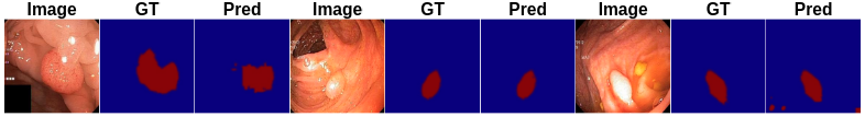
Figure S3: Qualitative visual results from Hyper-Kvasir testing set (red = anomaly).

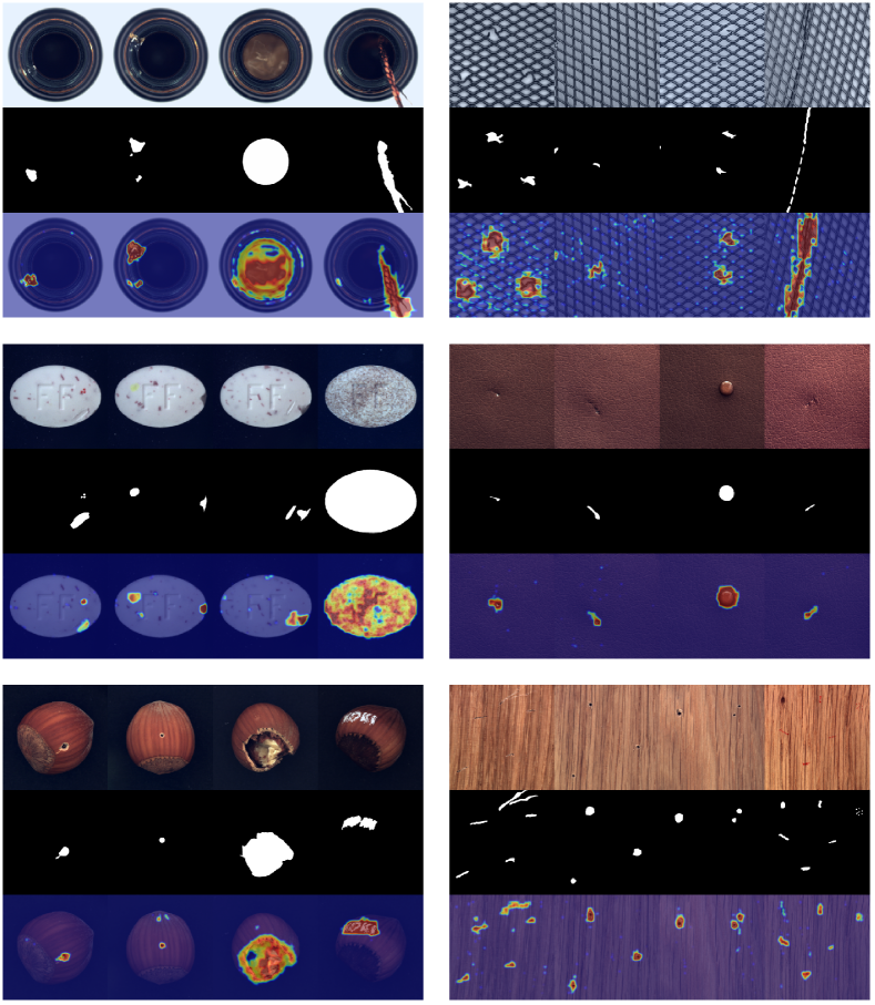
Figure S4: Qualitative results of our anomaly localisation results on the MVTec AD testing set (red = high probability of anomaly).

References

- Abati et al. (2019) Abati, D.; et al. 2019. Latent space autoregression for novelty detection. In Proceedings of the IEEE Conference on Computer Vision and Pattern Recognition, 481–490.
- Akcay et al. (2018) Akcay, S.; et al. 2018. Ganomaly: Semi-supervised anomaly detection via adversarial training. In Asian conference on computer vision, 622–637. Springer.
- Akçay et al. (2019) Akçay, S.; et al. 2019. Skip-ganomaly: Skip connected and adversarially trained encoder-decoder anomaly detection. In 2019 International Joint Conference on Neural Networks (IJCNN), 1–8.
- Baur et al. (2018) Baur, C.; Wiestler, B.; Albarqouni, S.; and Navab, N. 2018. Deep autoencoding models for unsupervised anomaly segmentation in brain MR images. In International MICCAI Brainlesion Workshop, 161–169. Springer.