Complexity of Linear Minimization
and Projection on Some Sets

Cyrille W. Combettes ^{1 3} cyrille@gatech.edu

Sebastian Pokutta ^{2 3} pokutta@zib.de

¹ School of Industrial and Systems Engineering, Georgia Institute of Technology, USA
² Institute of Mathematics, Technische Universität Berlin, Germany
³ Department for AI in Society, Science, and Technology, Zuse Institute Berlin, Germany

Abstract

The Frank-Wolfe algorithm is a method for constrained optimization that relies on linear minimizations, as opposed to projections. Therefore, a motivation put forward in a large body of work on the Frank-Wolfe algorithm is the computational advantage of solving linear minimizations instead of projections. However, the discussions supporting this advantage are often too succinct or incomplete. In this paper, we review the complexity bounds for both tasks on several sets commonly used in optimization. Projection methods onto the $\ell_{p}$-ball, $p\in\left]1,2\right[\cup\left]2,+\infty\right[$, and the Birkhoff polytope are also proposed.

1 Introduction

We consider the constrained optimization problem

$$\min_{x\in\mathcal{C}}f(x),$$ (1)

where $\mathcal{C}\subset\mathbb{R}^{n}$ is a compact convex set and $f\colon\mathbb{R}^{n}\rightarrow\mathbb{R}$ is a smooth function. Among all general purpose methods addressing problem (1), the Frank-Wolfe algorithm [17], a.k.a. conditional gradient algorithm [41], has the particularity of never requiring projections onto $\mathcal{C}$. It uses linear minimizations over $\mathcal{C}$ instead and is therefore often referred to as a projection-free algorithm in the literature, in the sense that it does not call for solutions to quadratic optimization subproblems.

Thus, a motivation put forward in a large body of work on the Frank-Wolfe algorithm is the computational advantage of solving linear minimizations instead of projections. However, only a few works actually provide examples. On the other hand, the complexities of linear minimizations over several sets are available in [27, 29, 19], but they do not always (accurately) discuss the complexities of the respective projections. Therefore, while it is intuitive that a linear minimization is simpler to solve than a projection in general, a complete quantitative assessment is necessary to properly motivate the projection-free property of the Frank-Wolfe algorithm.

Contributions.

We review the complexity bounds of linear minimizations and projections on several sets commonly used in optimization: the standard simplex, the $\ell_{p}$-balls for $p\in\left[1,+\infty\right]$, the nuclear norm-ball, the flow polytope, the Birkhoff polytope, and the permutahedron. These sets are selected because linear minimizations or projections can be solved very efficiently, rather than by resorting to a general purpose method, in which case the analysis is less interesting. We also propose two methods for projecting onto the $\ell_{p}$-ball and the Birkhoff polytope respectively, and we analyze their complexity. Computational experiments for the $\ell_{1}$-ball and the nuclear norm-ball are presented.

Remark 1.1.

We would like to stress that, while it is possible that a projection-based algorithm requires less iterations than the Frank-Wolfe algorithm to find a solution to problem (1), our goal here is to demonstrate its advantage in terms of per-iteration complexity. We discuss the Frank-Wolfe algorithm and some successful applications in Section 2.2.

2 Preliminaries

2.1 Notation and definitions

We work in the Euclidean space $\mathbb{R}^{n}$ or $\mathbb{R}^{m\times n}$ equipped with the standard scalar product $\langle x,y\rangle=x^{\top}y$ or $\langle X,Y\rangle=\operatorname{tr}(X^{\top}Y)$. We denote by $\|\cdot\|$ the norm induced by the scalar product, i.e., the $\ell_{2}$-norm $\|\cdot\|_{2}$ or the Frobenius norm $\|\cdot\|_{\operatorname{F}}$ respectively. For any closed convex set $\mathcal{C}\subset\mathbb{R}^{n}$, the projection operator onto $\mathcal{C}$, the distance function to $\mathcal{C}$, and the diameter of $\mathcal{C}$, all with respect to $\|\cdot\|$, are denoted by $\operatorname{proj}(\cdot,\mathcal{C})$, $\operatorname{dist}(\cdot,\mathcal{C})$, and $\operatorname{diam}(\mathcal{C})$ respectively.

For every $i,j\in\mathbb{N}$ such that $i\leqslant j$, the brackets $\llbracket i,j\rrbracket$ denote the set of integers between (and including) $i$ and $j$. For all $x\in\mathbb{R}^{n}$ and $i,j\in\llbracket 1,n\rrbracket$ such that $i\leqslant j$, $[x]_{i}$ denotes the $i$-th entry of $x$ and $[x]_{i:j}=([x]_{i},\ldots,[x]_{j})^{\top}\in\mathbb{R}^{j-i+1}$. The signum function is $\operatorname{sign}\colon\lambda\in\mathbb{R}\mapsto 1$ if $\lambda>0$, $-1$ if $\lambda<0$, and $0$ if $\lambda=0$. The characteristic function of an event $E$ is $\mathds{1}_{E}=1$ if $E$ is true, else $0$. The indicator function of a set $\mathcal{C}\subset\mathbb{R}^{n}$ is $\iota_{\mathcal{C}}\colon x\in\mathbb{R}^{n}\mapsto 0$ if $x\in\mathcal{C}$, else $+\infty$. Operations on vectors in $\mathbb{R}^{n}$, such as $\operatorname{sign}(x),|x|,x^{p},\max\{x,y\},xy$, that are conventionally applied to scalars, are carried out entrywise and return a vector in $\mathbb{R}^{n}$. The shape of $0$ and $1$ will be clear from context, i.e., a scalar or a vector. The identity matrix in $\mathbb{R}^{n\times n}$ is denoted by $I_{n}$. The matrix with all ones in $\mathbb{R}^{m\times n}$ is denoted by $J_{m,n}$, and by $J_{n}$ if $m=n$.

We adopt the real-number infinite-precision model of computation. The complexity of a computational task is the number of arithmetic operations necessary to execute it. We ran the experiments on a laptop under Linux Ubuntu 20.04 with Intel Core i7-10750H. The code is available at https://github.com/cyrillewcombettes/complexity.

2.2 The Frank-Wolfe algorithm

The Frank-Wolfe algorithm (FW) [17], a.k.a. conditional gradient algorithm [41], is a first-order projection-free algorithm for solving constrained optimization problems (1). It is presented in Algorithm 1.

Algorithm 1 Frank-Wolfe (FW)

0:  Start point $x_{0}\in\mathcal{C}$, step-size strategy $(\gamma_{t})_{t\in\mathbb{N}}\subset\left[0,1\right]$.

1:  for $t=0$ to $T-1$ do

2:     $v_{t}\leftarrow\operatorname*{\mathrm{arg\,min}}\limits_{v\in\mathcal{C}}\,\langle v,\nabla f(x_{t})\rangle$

3:     $x_{t+1}\leftarrow x_{t}+\gamma_{t}(v_{t}-x_{t})$

4:  end for

At each iteration, FW minimizes the linear approximation of $f$ at $x_{t}$ over $\mathcal{C}$ (Line 2), i.e.,

$$\min_{v\in\mathcal{C}}f(x_{t})+\langle v-x_{t},\nabla f(x_{t})\rangle,$$

and then moves in the direction of a solution $v_{t}\in\mathcal{C}$ with a step-size $\gamma_{t}\in\left[0,1\right]$ (Line 3). This ensures that the new iterate $x_{t+1}=(1-\gamma_{t})x_{t}+\gamma_{t}v_{t}\in\mathcal{C}$ is feasible by convexity, and there is no need for a projection back onto $\mathcal{C}$. For this projection-free property, FW has encountered numerous applications, including solving traffic assignment problems [39], performing video co-localization [30], or, e.g., developing adversarial attacks [6].

When $f$ is convex, FW converges at a rate $f(x_{t})-\min_{\mathcal{C}}f=\mathcal{O}(1/t)$ for different step-size strategies [17, 15, 29], which is optimal in general [5, 29]. Faster rates can be established under additional assumptions on the properties of $f$ or the geometry of $\mathcal{C}$ [41, 23, 20, 31]. Recently, several variants have also been developed to improve its performance [36, 38, 21, 18, 4, 9]. When $f$ is nonconvex, [35] showed that FW converges to a stationary point at a rate $\mathcal{O}(1/\sqrt{t})$ in the gap $\max_{v\in\mathcal{C}}\langle x_{t}-v,\nabla f(x_{t})\rangle$ [28], which has inspired a line of work in stochastic optimization [48, 52, 51, 10, 53].

Lastly, note that FW is also popular for the natural sparsity of its iterates with respect to the vertices of $\mathcal{C}$, as $x_{t}\in\operatorname{conv}\{x_{0},v_{0},\ldots,v_{t-1}\}$ [7, 26, 37, 43, 8].

3 Projections versus linear minimizations

The Frank-Wolfe algorithm avoids projections by computing linear minimizations instead. In Table 1, we summarize the complexities of a linear minimization and a (Euclidean) projection on several sets commonly used in optimization. That is, we compare the complexities of solving

$$\min_{x\in\mathcal{C}}\,\langle x,y\rangle\quad\text{and}\quad\min_{x\in\mathcal{C}}\|x-y\|.$$ (2)

When an exact solution cannot be computed directly, we compare to the complexity of finding an $\varepsilon$-approximate solution; note that the two objectives in (2) are homogeneous. For the projection problem, it means to solve $\min_{x\in\mathcal{C}}\|x-y\|^{2}$ using any method but the Frank-Wolfe algorithm, since it would go against the purpose of this paper. Note however that the Frank-Wolfe algorithm can generate a solution with complexity $\mathcal{O}(\operatorname{iter}(\mathcal{C})\operatorname{diam}(\mathcal{C})^{2}/\varepsilon^{2})$, where $\operatorname{iter}(\mathcal{C})$ denotes the complexity of an iteration, which amounts to that of a linear minimization over $\mathcal{C}$. When addressing problem (1), solving projection subproblems via the Frank-Wolfe algorithm is known as conditional gradient sliding [38].

Table 1: Complexities of linear minimizations and (Euclidean) projections on some sets commonly used in optimization. We denote by $x^{*}$ a solution, $\rho=p\sup_{t\in\mathbb{N}}\|x_{t}\|_{2(p-1)}^{p-1}\|x_{t}\|_{2}<+\infty$ where $(x_{t})_{t\in\mathbb{N}}$ is the sequence generated by Algorithm 2, by $\nu$ and $\sigma_{1}$ the number of nonzero entries and the top singular value of $-Y$ respectively, and by $\varepsilon>0$ the additive error in the objective of (2) when an approximate solution is computed. The constant $d_{z}$ is defined in (12) and $\tilde{\mathcal{O}}$ hides polylogarithmic factors in $m$ and $n$.

Set $\mathcal{C}$	Linear minimization	Projection	Reference
$\ell_{p}$-ball, $p\in\{1,2,+\infty\}$	$\mathcal{O}(n)$	$\mathcal{O}(n)$	Sections 3.1--3.2
$\ell_{p}$-ball, $p\in\left]1,2\right[\cup\left]2,+\infty\right[$	$\mathcal{O}(n)$	$\mathcal{O}(n\rho^{2}\|y-x^{*}\|_{2}^{2}/\varepsilon^{2})$	Section 3.3
Nuclear norm-ball	$\mathcal{O}(\nu\ln(m+n)\sqrt{\sigma_{1}}/\sqrt{\varepsilon})$	$\mathcal{O}(mn\min\{m,n\})$	Section 3.4
Flow polytope	$\mathcal{O}(m+n)$	$\tilde{\mathcal{O}}(m^{3}n+n^{2})$	Section 3.5
Birkhoff polytope	$\mathcal{O}(n^{3})$	$\mathcal{O}(n^{2}d_{z}^{2}/\varepsilon^{2})$	Section 3.6
Permutahedron	$\mathcal{O}(n\ln(n))$	$\mathcal{O}(n\ln(n)+n)$	Section 3.7

We now provide details for the complexities reported in Table 1. Slightly abusing notation though we may have $\operatorname{card}(\operatorname*{\mathrm{arg\,min}}_{x\in\mathcal{C}}\langle x,y\rangle)>1$, we write $\operatorname*{\mathrm{arg\,min}}_{x\in\mathcal{C}}\langle x,y\rangle=x^{*}$ instead of $\operatorname*{\mathrm{arg\,min}}_{x\in\mathcal{C}}\langle x,y\rangle\ni x^{*}$.

3.1 The $\ell_{1}$-ball and the standard simplex

Let $\{e_{1},\ldots,e_{n}\}$ denote the standard basis in $\mathbb{R}^{n}$. The $\ell_{1}$-ball is

$$\{x\in\mathbb{R}^{n}\mid\|x\|_{1}\leqslant 1\}=\left\{x\in\mathbb{R}^{n}\;\middle|\;\sum_{i=1}^{n}|[x]_{i}|\leqslant 1\right\}=\operatorname{conv}\{\pm e_{1},\ldots,\pm e_{n}\},$$

and the standard simplex is

$$\Delta_{n}=\{x\in\mathbb{R}^{n}\mid\langle x,1\rangle=1,x\geqslant 0\}=\operatorname{conv}\{e_{1},\ldots,e_{n}\}.$$

A projection onto the $\ell_{1}$-ball amounts to computing a projection onto the standard simplex, for which the most efficient algorithms have a complexity $\mathcal{O}(n)$; see [12] for a review. On the other hand, linear minimizations are available in closed form: for all $y\in\mathbb{R}^{n}$,

$$\operatorname*{\mathrm{arg\,min}}_{x\in\Delta_{n}}\,\langle x,y\rangle=e_{i_{\min}}\quad\text{and}\quad\operatorname*{\mathrm{arg\,min}}_{\|x\|_{1}\leqslant 1}\,\langle x,y\rangle=-\operatorname{sign}([y]_{i_{\max}})e_{i_{\max}},$$

where $i_{\min}\in\operatorname*{\mathrm{arg\,min}}_{i\in\llbracket 1,n\rrbracket}[y]_{i}$ and $i_{\max}\in\operatorname*{\mathrm{arg\,max}}_{i\in\llbracket 1,n\rrbracket}|[y]_{i}|$. Thus, while their complexities can both be written $\mathcal{O}(n)$, in practice linear minimizations are much simpler to solve than projections. Figure 1 presents a computational comparison. The results are averaged over $5$ runs and the shaded areas represent $\pm 1$ standard deviation.

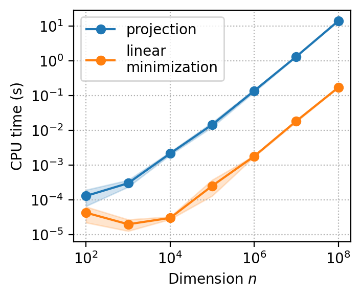
Figure 1: Solving a linear minimization and a projection on the $\ell_{1}$-ball. The input vector $y\in\mathbb{R}^{n}$ is generated by sampling entries from the standard normal distribution and the projection method is [12, Fig. 2], which is state-of-the-art in practice [12, Tab. 3]. In this situation, the plots suggest that linear minimizations are about $100\times$ faster to solve than projections when $n$ is large enough.

3.2 The $\ell_{2}$-ball and the $\ell_{\infty}$-ball

For all $x\in\mathbb{R}^{n}$, $\|x\|_{2}=\sqrt{\sum_{i=1}^{n}[x]_{i}^{2}}$ and $\|x\|_{\infty}=\max_{i\in\llbracket 1,n\rrbracket}|[x]_{i}|$. Here, linear minimizations have no significant advantage over projections as they are all available in closed form. For all $y\in\mathbb{R}^{n}$,

$$\operatorname*{\mathrm{arg\,min}}_{\|x\|_{2}\leqslant 1}\,\langle x,y\rangle=-\frac{y}{\|y\|_{2}}\quad\text{and}\quad\operatorname*{\mathrm{arg\,min}}_{\|x\|_{2}\leqslant 1}\|x-y\|_{2}=\frac{y}{\max\{\|y\|_{2},1\}},$$

and

$$\operatorname*{\mathrm{arg\,min}}_{\|x\|_{\infty}\leqslant 1}\,\langle x,y\rangle=-\operatorname{sign}(y)\quad\text{and}\quad\operatorname*{\mathrm{arg\,min}}_{\|x\|_{\infty}\leqslant 1}\|x-y\|_{2}=\operatorname{sign}(y)\min\{|y|,1\}.$$

3.3 The $\ell_{p}$-balls for $p\in\left]1,+\infty\right[$

Let $p\in\left]1,+\infty\right[$. The $\ell_{p}$-ball is

$$\{x\in\mathbb{R}^{n}\mid\|x\|_{p}\leqslant 1\}=\left\{x\in\mathbb{R}^{n}\;\middle|\;\left(\sum_{i=1}^{n}|[x]_{i}|^{p}\right)^{1/p}\leqslant 1\right\}.$$

Linear minimizations are available in closed form: by duality, for all $y\in\mathbb{R}^{n}$,

$$\operatorname*{\mathrm{arg\,min}}_{\|x\|_{p}\leqslant 1}\,\langle x,y\rangle=-\nabla\|\cdot\|_{q}(y)=-\frac{\operatorname{sign}(y)|y|^{q-1}}{\|y\|_{q}^{q-1}},$$

where $q=p/(p-1)\in\left]1,+\infty\right[$. To the best of our knowledge, there is no projection method specific to the $\ell_{p}$-ball when $p\in\left]1,2\right[\cup\left]2,+\infty\right[$. We use [11, Alg. 6.5], a Haugazeau-like algorithm [25] for projecting onto the intersection of sublevel sets of convex functions. For a single sublevel set, the problem reads

$$\min_{x\in\mathbb{R}^{n}}\; \|x-y\|_{2}^{2}$$ (3)

s.t. $$g(x)\leqslant 0,$$

and we assume that $g\colon\mathbb{R}^{n}\to\mathbb{R}$ is convex and differentiable for ease of exposition. In our case, $g=\|\cdot\|_{p}^{p}-1$. Alternatively, one could use a Lagrange multiplier to formulate (3) as a strongly convex unconstrained problem, but finding the corresponding multiplier may require a considerable effort of tuning; also note that information is usually given in the form $g(x)\leqslant 0$ rather than in the form of a Lagrange multiplier. The method is presented in Algorithm 2, where for all $a,b\in\mathbb{R}^{n}$,

$$H(a,b)=\{x\in\mathbb{R}^{n}\mid\langle x-b,a-b\rangle\leqslant 0\},$$

and $z_{t}$ is the projection of $x_{t}$ onto $\{x\in\mathbb{R}^{n}\mid g(x_{t})+\langle x-x_{t},\nabla g(x_{t})\rangle\leqslant 0\}=H(x_{t},z_{t})$. If $g(x_{t})\leqslant 0$, then $x_{t+s}=x^{*}$ for all $s\in\mathbb{N}$ [11, Prop. 3.1], where $x^{*}$ is the solution to problem (3).

Algorithm 2 Haugazeau-like for problem (3)

0:  Point to project $y\in\mathbb{R}^{n}$.

1:  $x_{0}\leftarrow y$

2:  for $t=0$ to $T-1$ do

3:     $z_{t}\leftarrow x_{t}-\displaystyle\frac{g(x_{t})}{\|\nabla g(x_{t})\|_{2}^{2}}\nabla g(x_{t})\mathds{1}_{\{g(x_{t})>0\}}$

4:     $x_{t+1}\leftarrow\operatorname{proj}(x_{0},H(x_{0},x_{t})\cap H(x_{t},z_{t}))$

5:  end for

The projection in Line 4 is available in closed form [25, Thm. 3-1]; see also [2, Cor. 29.25]. The complexity of an iteration of Algorithm 2 is $\mathcal{O}(n)$. We propose in Theorem 3.1 the convergence rate of Algorithm 2, based on a key result from [1, Thm. 7.12]. A convergence rate is also proposed in [46], however it uses a stronger assumption and has a minor error in the exponent of the constant.

Theorem 3.1.

Let $g\colon\mathbb{R}^{n}\rightarrow\mathbb{R}$ be a differentiable convex function and $\mathcal{C}=\{x\in\mathbb{R}^{n}\mid g(x)\leqslant 0\}$, and suppose that there exists $\hat{x}\in\mathcal{C}$ such that $g(\hat{x})<0$. Consider Algorithm 2 and let $x^{*}=\operatorname{proj}(x_{0},\mathcal{C})$. Then, for all $t\in\mathbb{N}$,

$$\|x^{*}-x_{0}\|_{2}^{2}-\|x_{t}-x_{0}\|_{2}^{2}\leqslant\frac{\max\{8\rho^{2},2\}\|x_{0}-x^{*}\|_{2}^{2}}{t+2},$$ (4)

and

$$\|x_{t}-x^{*}\|_{2}\leqslant\frac{\max\{2\sqrt{2}\rho,\sqrt{2}\}\|x_{0}-x^{*}\|_{2}}{\sqrt{t+2}},$$ (5)

where $\rho=(-1/g(\hat{x}))\sup_{t\in\mathbb{N}}\|\nabla g(x_{t})\|_{2}\|x_{t}-\hat{x}\|_{2}<+\infty$.

Proof.

First, note that by [11, Prop. 3.1], for all $t\in\mathbb{N}$,

$$\|x_{t}-x_{0}\|_{2}\leqslant\|x_{t+1}-x_{0}\|_{2}\leqslant\|x^{*}-x_{0}\|_{2}.$$ (6)

We prove by induction that (4) holds for all $t\in\mathbb{N}$. The base case $t=0$ is trivial. Suppose that (4) holds at iteration $t\in\mathbb{N}$. Since $x_{t+1}\in H(x_{0},x_{t})$ and $x_{t+1}\in H(x_{t},z_{t})$, we have

$$\|x_{t+1}-x_{0}\|_{2}^{2}-\|x_{t}-x_{0}\|_{2}^{2} =\|x_{t+1}-x_{t}\|_{2}^{2}+2\langle x_{t+1}-x_{t},x_{t}-x_{0}\rangle$$

$$\geqslant\|x_{t+1}-x_{t}\|_{2}^{2}$$

$$\geqslant\operatorname{dist}(x_{t},H(x_{t},z_{t}))^{2}.$$ (7)

By [1, Thm. 7.12],

$$\operatorname{dist}(x_{t},\mathcal{C})\leqslant\rho\operatorname{dist}(x_{t},H(x_{t},z_{t})),$$ (8)

where $\rho=(-1/g(\hat{x}))\sup_{t\in\mathbb{N}}\|\nabla g(x_{t})\|_{2}\|x_{t}-\hat{x}\|_{2}$, and $\rho<+\infty$ because $(x_{t})_{t\in\mathbb{N}}$ converges [2, Cor. 30.9]. Now, $x^{*}=\operatorname{proj}(x_{0},\mathcal{C})$ so $\mathcal{C}\subset H(x_{0},x^{*})$. We can assume that $x_{t}\neq x^{*}$, so $x_{t}\notin H(x_{0},x^{*})$ by (6). By [2, Ex. 29.20],

$$\operatorname{dist}(x_{t},H(x_{0},x^{*}))=\frac{\langle x_{t}-x^{*},x_{0}-x^{*}\rangle}{\|x_{0}-x^{*}\|_{2}}.$$

Thus,

$$\operatorname{dist}(x_{t},\mathcal{C}) \geqslant\operatorname{dist}(x_{t},H(x_{0},x^{*}))$$

$$=\frac{\langle x_{t}-x^{*},x_{0}-x^{*}\rangle}{\|x_{0}-x^{*}\|_{2}}$$

$$=\frac{\langle x_{t}-x_{0},x_{0}-x^{*}\rangle+\|x_{0}-x^{*}\|_{2}^{2}}{\|x_{0}-x^{*}\|_{2}}$$

$$\geqslant\|x_{0}-x^{*}\|_{2}-\|x_{t}-x_{0}\|_{2}$$

$$=\|x_{0}-x^{*}\|_{2}-\sqrt{\|x^{*}-x_{0}\|_{2}^{2}-(\|x^{*}-x_{0}\|_{2}^{2}-\|x_{t}-x_{0}\|_{2}^{2})}$$ (9)

$$\geqslant 0,$$

where we used the Cauchy-Schwarz inequality in the second inequality and (6) in the last inequality. Let $\varepsilon_{s}=\|x^{*}-x_{0}\|_{2}^{2}-\|x_{s}-x_{0}\|_{2}^{2}$ for $s\in\{t,t+1\}$. Combining (7)–(9),

$$\varepsilon_{t+1} \leqslant\varepsilon_{t}-\frac{1}{\rho^{2}}\left(\|x_{0}-x^{*}\|_{2}-\sqrt{\|x^{*}-x_{0}\|_{2}^{2}-\varepsilon_{t}}\right)^{2}.$$

Since $\sqrt{\alpha-\beta}\leqslant\sqrt{\alpha}-\beta/(2\sqrt{\alpha})$ for all $\alpha\geqslant\beta>0$, we obtain

$$\varepsilon_{t+1} \leqslant\varepsilon_{t}-\frac{1}{\rho^{2}}\left(\|x_{0}-x^{*}\|_{2}-\left(\|x^{*}-x_{0}\|_{2}-\frac{\varepsilon_{t}}{2\|x^{*}-x_{0}\|_{2}}\right)\right)^{2}$$

$$=\left(1-\frac{\varepsilon_{t}}{4\rho^{2}\|x^{*}-x_{0}\|_{2}^{2}}\right)\varepsilon_{t}.$$

Let $\kappa=\max\{8\rho^{2},2\}\|x_{0}-x^{*}\|_{2}^{2}$. We have $\varepsilon_{t}\leqslant\kappa/(t+2)$ by the induction hypothesis, so

$$\varepsilon_{t+1} \leqslant\left(1-\frac{\varepsilon_{t}}{\kappa/2}\right)\varepsilon_{t}$$

$$\leqslant\begin{cases}\displaystyle\frac{\kappa/2}{t+2}&\text{if }\displaystyle\varepsilon_{t}\leqslant\frac{\kappa/2}{t+2}\\ \displaystyle\left(1-\frac{1}{t+2}\right)\frac{\kappa}{t+2}&\text{if }\displaystyle\varepsilon_{t}\geqslant\frac{\kappa/2}{t+2}\end{cases}$$

$$\leqslant\frac{\kappa}{t+3}.$$

We conclude that (4) holds for all $t\in\mathbb{N}$. Then, for all $t\in\mathbb{N}$,

$$\|x_{t}-x^{*}\|_{2}^{2} =\|x^{*}-x_{0}\|_{2}^{2}-\|x_{t}-x_{0}\|_{2}^{2}+2\langle x^{*}-x_{t},x_{0}-x_{t}\rangle$$

$$\leqslant\|x^{*}-x_{0}\|_{2}^{2}-\|x_{t}-x_{0}\|_{2}^{2},$$

because $x^{*}\in H(x_{0},x_{t})$, since $\mathcal{C}\subset H(x_{0},x_{t})$ [11, Prop. 5.2]. This proves (5). ∎

In our case, $g=\|\cdot\|_{p}^{p}-1$ and $g(0)=-1<0$, so Theorem 3.1 holds with

$$\rho=\sup_{t\in\mathbb{N}}\|\nabla g(x_{t})\|_{2}\|x_{t}\|_{2}=p\sup_{t\in\mathbb{N}}\|x_{t}\|_{2(p-1)}^{p-1}\|x_{t}\|_{2}<+\infty.$$

Therefore, the complexity of an $\varepsilon$-approximate projection onto the $\ell_{p}$-ball is $\mathcal{O}(n\rho^{2}\|y-x^{*}\|_{2}^{2}/\varepsilon^{2})$.

Remark 3.2.

If $p\in\left[1,+\infty\right[\cap\mathbb{Q}$, another option, although probably less practical, is to formulate the projection problem as a conic quadratic program and to obtain an $\varepsilon$-approximate solution using an interior-point algorithm, with complexity $\mathcal{O}(\operatorname{poly}(n)\ln(1/\varepsilon))$ [3].

3.4 The nuclear norm-ball

This is probably the most popular example of the computational advantage of linear minimizations over projections in the literature. The nuclear norm, a.k.a. trace norm, of a matrix is the sum of its singular values and serves as a convex surrogate for the rank constraint [16]. The nuclear norm-ball is the convex hull of rank-$1$ matrices:

$$\{X\in\mathbb{R}^{m\times n}\mid\|X\|_{\operatorname{nuc}}\leqslant 1\}=\operatorname{conv}\{uv^{\top}\mid u\in\mathbb{R}^{m},v\in\mathbb{R}^{n},\|u\|_{2}=\|v\|_{2}=1\}.$$

For all $Y\in\mathbb{R}^{m\times n}$,

$$\operatorname*{\mathrm{arg\,min}}_{\|X\|_{\operatorname{nuc}}\leqslant 1}\|X-Y\|_{\operatorname{F}}=U\operatorname{diag}(\hat{\sigma})V^{\top},$$

where $Y=U\operatorname{diag}(\sigma)V^{\top}$ is the singular value decomposition (SVD) of $Y$, $(U,\sigma,V)\in\mathbb{R}^{m\times k}\times\mathbb{R}^{k}\times\mathbb{R}^{n\times k}$, $k=\min\{m,n\}$, and $\hat{\sigma}$ is the projection of $\sigma$ onto the standard simplex $\Delta_{k}$. The SVD can be computed with complexity $\mathcal{O}(mn\min\{m,n\}+\min\{m^{3},n^{3}\})$ using the Golub-Reinsch algorithm or the $R$-SVD algorithm [22, Fig. 8.6.1]. On the other hand, a linear minimization requires only a truncated SVD:

$$\operatorname*{\mathrm{arg\,min}}_{\|X\|_{\operatorname{nuc}}\leqslant 1}\,\langle X,Y\rangle=\operatorname*{\mathrm{arg\,max}}_{\|u\|_{2}=\|v\|_{2}=1}\operatorname{tr}((uv^{\top})^{\top}(-Y))=\operatorname*{\mathrm{arg\,max}}_{\|u\|_{2}=\|v\|_{2}=1}u^{\top}(-Y)v=uv^{\top},$$

where $u$ and $v$ are the top left and right singular vectors of $-Y$. A pair of unit vectors $(u,v)\in\mathbb{R}^{m}\times\mathbb{R}^{n}$ satisfying $\sigma_{1}-u^{\top}(-Y)v\leqslant\varepsilon$ with high probability can be obtained using the Lanczos algorithm with complexity $\mathcal{O}(\nu\ln(m+n)\sqrt{\sigma_{1}}/\sqrt{\varepsilon})$, where $\sigma_{1}$ and $\nu$ denote the top singular value and the number of nonzero entries in $-Y$ respectively [29, 33]. Note that $\nu\leqslant mn$ and that in many applications of interest, e.g., in recommender systems, $\nu\ll mn$.

In practice, the package ARPACK [40] is often used to compute the top pair of singular vectors. Furthermore, if the input matrix $Y$ is symmetric, then the package LOBPCG [32] can be particularly efficient. Figure 2 illustrates both cases, where linear minimizations are solved to machine precision. The results are averaged over $5$ runs and the shaded areas represent $\pm 1$ standard deviation.

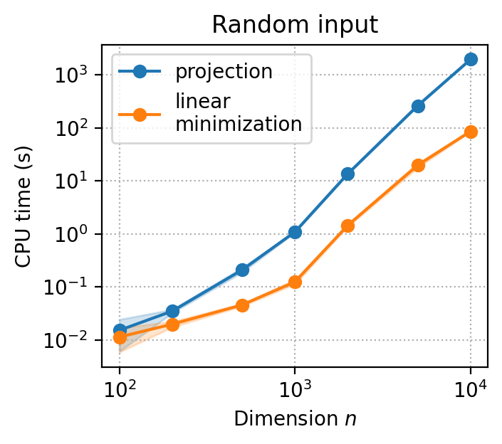
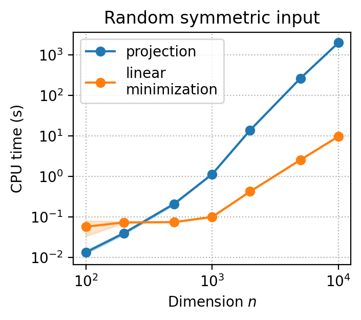
Figure 2: Solving a linear minimization and a projection on the nuclear norm-ball. A matrix $Y\in\mathbb{R}^{n\times n}$ is generated by sampling entries from the standard normal distribution. The full and truncated SVDs are computed using the functions svd and svds from the Python packages numpy.linalg [24] and scipy.sparse.linalg [50] respectively. The function svds is used with tol=0. Left: The input is $Y$ and the function svds is used with solver=‘arpack’. Right: The input is the symmetric matrix $(Y+Y^{\top})/2$ and the function svds is used with solver=‘lobpcg’. We see that the ratio of CPU times increases as $n$ increases.

3.5 The flow polytope

Let $G$ be a single-source single-sink directed acyclic graph (DAG) with $m$ vertices and $n$ edges. Index by $\llbracket 1,m\rrbracket$ the set of vertices such that the edges are directed from a smaller to a larger vertex index; this can be achieved with complexity $\mathcal{O}(m+n)$ via topological sort [13, Sec. 22.4]. Let $A_{G}\in\mathbb{R}^{m\times n}$ be the incidence matrix of $G$. The flow polytope induced by $G$ is

$$\mathcal{F}_{G}=\{x\in\mathbb{R}^{n}\mid A_{G}x=(-1,0,\ldots,0,1)^{\top},x\geqslant 0\},$$

i.e., $\mathcal{F}_{G}$ is the set of unit flows $x\in\mathbb{R}^{n}$ on $G$, where $[x]_{i}\geqslant 0$ denotes the flow going through edge $i$. Thus, for all $y\in\mathbb{R}^{n}$, $\operatorname*{\mathrm{arg\,min}}_{x\in\mathcal{F}_{G}}\langle x,y\rangle$ is a flow $x\in\{0,1\}^{n}$ identifying a shortest path on $G$ weighted by $y$. Its computation has complexity $\mathcal{O}(m+n)$ [13, Sec. 24.2]. This is significantly cheaper than the complexity $\tilde{\mathcal{O}}(m^{3}n+n^{2})$ of a projection [49, Thm. 20], where $\tilde{\mathcal{O}}$ hides polylogarithmic factors.

3.6 The Birkhoff polytope

The Birkhoff polytope, a.k.a. assignment polytope, is the set of doubly stochastic matrices

$$\mathcal{B}_{n}=\{X\in\mathbb{R}^{n\times n}\mid X1=1,X^{\top}1=1,X\geqslant 0\}.$$

It is the convex hull of the permutation matrices and arises in matching, ranking, and seriation problems. Linear minimizations can be solved with complexity $\mathcal{O}(n^{3})$ using the Hungarian algorithm [34]. To the best of our knowledge, there is no projection method specific to the Birkhoff polytope so we propose one here. Let $Y\in\mathbb{R}^{n\times n}$. By reshaping it into a vector $y\in\mathbb{R}^{n^{2}}$, projecting $Y$ onto the Birkhoff polytope is equivalent to solving

$$\begin{aligned} \min_{x\in\mathbb{R}^{n^{2}}}\;&\|x-y\|_{2}^{2}\\ \text{s.t.}\;&Ax=1\\ &x\geqslant 0,\end{aligned}\quad\quad\text{where}\quad A=\begin{pmatrix}1^{\top}&0^{\top}&\cdots&0^{\top}\\ 0^{\top}&\ddots&\ddots&\vdots\\ \vdots&\ddots&\ddots&0^{\top}\\ 0^{\top}&\cdots&0^{\top}&1^{\top}\\ I_{n}&\cdots&\cdots&I_{n}\end{pmatrix}\in\mathbb{R}^{2n\times n^{2}}.$$ (10)

This can again be reformulated as

$$\min_{x\in\mathbb{R}^{n^{2}}}\left(\iota_{\mathcal{K}}(x)+\frac{1}{2}\|x-y\|_{2}^{2}\right)+\left(\iota_{\mathcal{A}}(x)+\frac{1}{2}\|x-y\|_{2}^{2}\right),$$ (11)

where $\mathcal{K}=\{x\in\mathbb{R}^{n^{2}}\mid x\geqslant 0\}$ and $\mathcal{A}=\{x\in\mathbb{R}^{n^{2}}\mid Ax=1\}$. That is, we split the constraints into two sets enjoying efficient projections. We can now apply the Douglas-Rachford algorithm [42] to problem (11). The method is presented in Algorithm 3; see Appendix A for details. Line 3 computes the projection of $u_{t}$ onto the affine subspace $\mathcal{A}$ and in Line 4 is computed a projection onto the nonnegative orthant $\mathcal{K}$. We can set $u=1/n\in\mathcal{A}$ and we denote by $A^{\dagger}\in\mathbb{R}^{n^{2}\times 2n}$ the Moore-Penrose inverse of $A$.

Algorithm 3 Douglas-Rachford for problem (11)

0:  Point to project $y\in\mathbb{R}^{n^{2}}$, start point $z_{0}\in\mathbb{R}^{n^{2}}$, offset point $u\in\mathcal{A}$.

1:  for $t=0$ to $T-1$ do

2:     $u_{t}\leftarrow\displaystyle\frac{z_{t}+y}{2}$

3:     $x_{t}\leftarrow u_{t}-A^{\dagger}A(u_{t}-u)$

4:     $z_{t+1}\leftarrow\max\left\{\displaystyle\frac{2x_{t}-z_{t}+y}{2},0\right\}+z_{t}-x_{t}$

5:  end for

The complexity of an iteration of Algorithm 3 is dominated by the matrix-vector multiplication in Line 3. We can assume that $A^{\dagger}A\in\mathbb{R}^{n^{2}\times n^{2}}$ is precomputed. In fact,

$$A^{\dagger}A=\frac{1}{n^{2}}\begin{pmatrix}B_{1}&B_{2}&\cdots&B_{2}\\ B_{2}&\ddots&\ddots&\vdots\\ \vdots&\ddots&\ddots&B_{2}\\ B_{2}&\cdots&B_{2}&B_{1}\\ \end{pmatrix}\in\mathbb{R}^{n^{2}\times n^{2}},\quad\text{where}\quad\begin{cases}B_{1}=nI_{n}+(n-1)J_{n}\in\mathbb{R}^{n\times n}\\ B_{2}=nI_{n}-J_{n}\in\mathbb{R}^{n\times n},\end{cases}$$

so $A^{\dagger}A$ is block circulant with circulant blocks (BCCB) and has only three distinct entries: $2n-1$, $n-1$, and $-1$. The expression of $A^{\dagger}A$ can be shown by checking that $A^{\dagger}=A^{\top}/n-J_{n^{2},2n}/(2n^{2})\in\mathbb{R}^{n^{2}\times 2n}$ using the necessary and sufficient Moore-Penrose conditions [47, Thm. 1]. Thus, the multiplication of $A^{\dagger}A$ and any vector $x\in\mathbb{R}^{n^{2}}$ can be performed with complexity $\mathcal{O}(n^{2})$. Indeed, it amounts to computing $(nI_{n}+(n-1)J_{n})[x]_{i:j}$ and $(nI_{n}-J_{n})[x]_{i:j}$ for every $(i,j)\in\{(kn+1,(k+1)n)\mid k\in\llbracket 0,n-1\rrbracket\}$, each of which has complexity $\mathcal{O}(n)$.

It remains to bound the number of iterations required to achieve $\varepsilon$-convergence. Let $x^{*}=\operatorname{proj}(y,\mathcal{A}\cap\mathcal{K})$ be the solution to problem (11), i.e., the projection of $Y$ onto the Birkhoff polytope after reshaping, and let $\bar{x}_{t}=(\sum_{s=0}^{t}x_{s})/(t+1)\in\mathcal{A}$ for all $t\in\mathbb{N}$. By [14, Thm. 1],

$$\|\bar{x}_{t}-x^{*}\|_{2}\leqslant\frac{\|z_{0}-z^{*}\|_{2}}{\sqrt{2(t+1)}},$$

where $z^{*}$ is a fixed point of $\operatorname{rprox}_{\iota_{\mathcal{K}}+(1/2)\|\cdot-y\|_{2}^{2}}\circ\operatorname{rprox}_{\iota_{\mathcal{A}}+(1/2)\|\cdot-y\|_{2}^{2}}$, $\operatorname{rprox}_{\varphi}=2\operatorname{prox}_{\varphi}-\operatorname{id}$, and $\operatorname{prox}_{\varphi}$ is the proximity operator of $\varphi$ [44]. Therefore, the complexity of an $\varepsilon$-approximate projection onto the Birkhoff polytope is $\mathcal{O}(n^{2}d_{z}^{2}/\varepsilon^{2})$, where

$$d_{z}=\|z_{0}-z^{*}\|_{2}.$$ (12)

3.7 The permutahedron

Let $\mathfrak{S}_{n}$ be the set of permutations on $\llbracket 1,n\rrbracket$ and $w\in\mathbb{R}^{n}$. The permutahedron induced by $w$ is the convex hull of all permutations of the entries in $w$, i.e.,

$$\mathcal{P}_{w}=\operatorname{conv}\{w_{\sigma}\in\mathbb{R}^{n}\mid w_{\sigma}=([w]_{\sigma_{1}},\ldots,[w]_{\sigma_{n}})^{\top},\sigma\in\mathfrak{S}_{n}\}.$$

It is related to the Birkhoff polytope via $\mathcal{P}_{w}=\{Xw\mid X\in\mathcal{B}_{n}\}$. With no loss of generality, we can assume that the weights are already sorted in ascending order: $[w]_{1}\leqslant\cdots\leqslant[w]_{n}$. Thus, for all $y\in\mathbb{R}^{n}$,

$$\operatorname*{\mathrm{arg\,min}}_{x\in\mathcal{P}_{w}}\,\langle x,y\rangle=w_{\sigma^{-1}},$$

where $\sigma$ satisfies $[y]_{\sigma_{1}}\geqslant\cdots\geqslant[y]_{\sigma_{n}}$. Sorting the entries of $y$ has complexity $\mathcal{O}(n\ln(n))$ [13]. A projection can be obtained with a slightly higher complexity $\mathcal{O}(n\ln(n)+n)$, by sorting the entries of $y$ and solving an isotonic regression problem [45].

Acknowledgment

Research reported in this paper was partially supported by the Research Campus MODAL funded by the German Federal Ministry of Education and Research under grant 05M14ZAM.

Appendix A An application of the Douglas-Rachford algorithm

Let $\mathcal{H}$ be a Euclidean space with norm $\|\cdot\|$ and denote by $\Gamma_{0}(\mathcal{H})$ the set of proper lower semicontinuous convex functions $\mathcal{H}\rightarrow\mathbb{R}\cup\{+\infty\}$. The Douglas-Rachford algorithm [42] can be used to solve

$$\min_{x\in\mathcal{H}}f(x)+g(x),$$

when $f,g\in\Gamma_{0}(\mathcal{H})$ satisfy $\operatorname*{\mathrm{arg\,min}}_{\mathcal{H}}(f+g)\neq\varnothing$ and $(\operatorname{ri}\operatorname{dom}f)\cap(\operatorname{ri}\operatorname{dom}g)\neq\varnothing$ [2], where $\operatorname{ri}$ and $\operatorname{dom}$ denote the relative interior of a set and the domain of a function respectively. It is presented in Algorithm 4. For every function $\varphi\in\Gamma_{0}(\mathcal{H})$, the proximity operator is $\operatorname{prox}_{\varphi}=\operatorname*{\mathrm{arg\,min}}_{x\in\mathcal{H}}\varphi(x)+(1/2)\|\cdot-x\|^{2}$ [44].

Algorithm 4 Douglas-Rachford

0:  Start point $z_{0}\in\mathcal{H}$.

1:  for $t=0$ to $T-1$ do

2:     $x_{t}\leftarrow\operatorname{prox}_{g}(z_{t})$

3:     $z_{t+1}\leftarrow\operatorname{prox}_{f}(2x_{t}-z_{t})+z_{t}-x_{t}$

4:  end for

We are interested in an application to problem (11), where $\mathcal{H}=\mathbb{R}^{n^{2}}$, $f=\iota_{\mathcal{K}}+(1/2)\|\cdot-y\|_{2}^{2}$, $g=\iota_{\mathcal{A}}+(1/2)\|\cdot-y\|_{2}^{2}$, $y\in\mathcal{H}$, $\mathcal{K}=\{x\in\mathbb{R}^{n^{2}}\mid x\geqslant 0\}$, $\mathcal{A}=\{x\in\mathbb{R}^{n^{2}}\mid Ax=1\}$, and $A\in\mathbb{R}^{2n\times n^{2}}$ is defined in (10). Problem (11) admits a (unique) solution since it is a projection problem onto the intersection of the closed convex sets $\mathcal{K}$ and $\mathcal{A}$, and $1/n\in(\operatorname{ri}\operatorname{dom}f)\cap(\operatorname{ri}\operatorname{dom}g)=(\operatorname{ri}\mathcal{K})\cap\mathcal{A}$ so the Douglas-Rachford algorithm is well defined here. We now show that it reduces to Algorithm 3. For all $t\in\mathbb{N}$,

$$x_{t} =\operatorname{prox}_{g}(z_{t})$$

$$=\operatorname*{\mathrm{arg\,min}}_{x\in\mathcal{H}}g(x)+\frac{1}{2}\|z_{t}-x\|_{2}^{2}$$

$$=\operatorname*{\mathrm{arg\,min}}_{x\in\mathcal{A}}\frac{1}{2}\|x-y\|_{2}^{2}+\frac{1}{2}\|x-z_{t}\|_{2}^{2}$$

$$=\operatorname*{\mathrm{arg\,min}}_{x\in\mathcal{A}}\left\|x-\frac{z_{t}+y}{2}\right\|_{2}^{2}$$

$$=\operatorname{proj}\left(\frac{z_{t}+y}{2},\mathcal{A}\right)$$

$$=\frac{z_{t}+y}{2}-A^{\dagger}A\left(\frac{z_{t}+y}{2}-u\right),$$

since $\operatorname{proj}(\cdot,\mathcal{A})=\cdot-A^{\dagger}A(\cdot-u)$, given any $u\in\mathcal{A}$ [2, Ex. 29.17]. Thus, Lines 2--3 in Algorithm 3 are equivalent to Line 2 in Algorithm 4. Similarly, Line 4 in Algorithm 3 is equivalent to Line 3 in Algorithm 4:

$$z_{t+1} =\operatorname{prox}_{f}(2x_{t}-z_{t})+z_{t}-x_{t}$$

$$=\operatorname*{\mathrm{arg\,min}}_{z\in\mathcal{H}}\left(f(z)+\frac{1}{2}\|2x_{t}-z_{t}-z\|_{2}^{2}\right)+z_{t}-x_{t}$$

$$=\operatorname*{\mathrm{arg\,min}}_{z\in\mathcal{K}}\left(\frac{1}{2}\|z-y\|_{2}^{2}+\frac{1}{2}\|z-(2x_{t}-z_{t})\|_{2}^{2}\right)+z_{t}-x_{t}$$

$$=\operatorname*{\mathrm{arg\,min}}_{z\in\mathcal{K}}\left\|z-\frac{2x_{t}-z_{t}+y}{2}\right\|_{2}^{2}+z_{t}-x_{t}$$

$$=\operatorname{proj}\left(\frac{2x_{t}-z_{t}+y}{2},\mathcal{K}\right)+z_{t}-x_{t}$$

$$=\max\left\{\frac{2x_{t}-z_{t}+y}{2},0\right\}+z_{t}-x_{t},$$

since $\operatorname{proj}(\cdot,\mathcal{K})=\max\{\cdot,0\}$.

References

- [1] H. H. Bauschke and J. M. Borwein. On projection algorithms for solving convex feasibility problems. SIAM Review, 38(3):367--426, 1996.
- [2] H. H. Bauschke and P. L. Combettes. Convex Analysis and Monotone Operator Theory in Hilbert Spaces. Springer, 2nd edition, 2017.
- [3] A. Ben-Tal and A. S. Nemirovski. Lectures on Modern Convex Optimization: Analysis, Algorithms, and Engineering Applications. Society for Industrial and Applied Mathematics, 2001.
- [4] G. Braun, S. Pokutta, and D. Zink. Lazifying conditional gradient algorithms. Journal of Machine Learning Research, 20(71):1--42, 2019.
- [5] M. D. Canon and C. D. Cullum. A tight upper bound on the rate of convergence of Frank-Wolfe algorithm. SIAM Journal on Control, 6(4):509--516, 1968.
- [6] J. Chen, D. Zhou, J. Yi, and Q. Gu. A Frank-Wolfe framework for efficient and effective adversarial attacks. In Proceedings of the 34th AAAI Conference on Artificial Intelligence, pages 3486--3494, 2020.
- [7] K. L. Clarkson. Coresets, sparse greedy approximation, and the Frank-Wolfe algorithm. ACM Transactions on Algorithms, 6(4):1--30, 2010.
- [8] C. W. Combettes and S. Pokutta. Revisiting the approximate Carathéodory problem via the Frank-Wolfe algorithm. arXiv preprint arXiv:1911.04415, 2019.
- [9] C. W. Combettes and S. Pokutta. Boosting Frank-Wolfe by chasing gradients. In Proceedings of the 37th International Conference on Machine Learning, pages 2111--2121, 2020.
- [10] C. W. Combettes, C. Spiegel, and S. Pokutta. Projection-free adaptive gradients for large-scale optimization. arXiv preprint arXiv:2009.14114, 2020.
- [11] P. L. Combettes. Strong convergence of block-iterative outer approximation methods for convex optimization. SIAM Journal on Control and Optimization, 38(2):538--565, 2000.
- [12] L. Condat. Fast projection onto the simplex and the ball. Mathematical Programming, 158(1):575--585, 2016.
- [13] T. H. Cormen, C. E. Leiserson, R. L. Rivest, and C. Stein. Introduction to Algorithms. MIT Press, 3rd edition, 2009.
- [14] D. Davis and W. Yin. Faster convergence rates of relaxed Peaceman-Rachford and ADMM under regularity assumptions. Mathematics of Operations Research, 42(3):783--805, 2017.
- [15] J. C. Dunn and S. Harshbarger. Conditional gradient algorithms with open loop step size rules. Journal of Mathematical Analysis and Applications, 62(2):432--444, 1978.
- [16] M. Fazel, H. Hindi, and S. P. Boyd. A rank minimization heuristic with application to minimum order system approximation. In Proceedings of the 2001 American Control Conference, pages 4734--4739, 2001.
- [17] M. Frank and P. Wolfe. An algorithm for quadratic programming. Naval Research Logistics Quarterly, 3(1--2):95--110, 1956.
- [18] R. M. Freund, P. Grigas, and R. Mazumder. An extended Frank-Wolfe method with ‘‘in-face’’ directions, and its application to low-rank matrix completion. SIAM Journal on Optimization, 27(1):319--346, 2017.
- [19] D. Garber. Projection-free Algorithms for Convex Optimization and Online Learning. Ph.D. thesis, Technion, 2016.
- [20] D. Garber and E. Hazan. Faster rates for the Frank-Wolfe method over strongly-convex sets. In Proceedings of the 32nd International Conference on Machine Learning, pages 541--549, 2015.
- [21] D. Garber and O. Meshi. Linear-memory and decomposition-invariant linearly convergent conditional gradient algorithm for structured polytopes. In Advances in Neural Information Processing Systems, volume 29, pages 1001--1009, 2016.
- [22] G. H. Golub and C. F. van Loan. Matrix Computations. Johns Hopkins University Press, 4th edition, 2013.
- [23] J. Guélat and P. Marcotte. Some comments on Wolfe’s ‘away step’. Mathematical Programming, 35(1):110--119, 1986.
- [24] C. R. Harris et al. Array programming with NumPy. Nature, 585(7825):357--362, 2020.
- [25] Y. Haugazeau. Sur les Inéquations Variationnelles et la Minimisation de Fonctionnelles Convexes. Thèse de doctorat, Université de Paris, 1968.
- [26] E. Hazan. Sparse approximate solutions to semidefinite programs. In Proceedings of the 8th Latin American Symposium on Theoretical Informatics, pages 306--316, 2008.
- [27] E. Hazan and S. Kale. Projection-free online learning. In Proceedings of the 29th International Conference on Machine Learning, 2012.
- [28] D. W. Hearn. The gap function of a convex program. Operations Research Letters, 1(2):67--71, 1982.
- [29] M. Jaggi. Revisiting Frank-Wolfe: Projection-free sparse convex optimization. In Proceedings of the 30th International Conference on Machine Learning, pages 427--435, 2013.
- [30] A. Joulin, K. Tang, and L. Fei-Fei. Efficient image and video co-localization with Frank-Wolfe algorithm. In European Conference on Computer Vision, pages 253--268, 2014.
- [31] T. Kerdreux, A. d’Aspremont, and S. Pokutta. Projection-free optimization on uniformly convex sets. In Proceedings of the 24th International Conference on Artificial Intelligence and Statistics, pages 19--27, 2021.
- [32] A. V. Knyazev, M. E. Argentati, I. Lashuk, and E. E. Ovtchinnikov. Block locally optimal preconditioned eigenvalue xolvers (BLOPEX) in hypre and PETSc. SIAM Journal on Scientific Computing, 29(5):2224--2239, 2007.
- [33] J. Kuczyński and H. Woźniakowski. Estimating the largest eigenvalue by the power and Lanczos algorithms with a random start. SIAM Journal on Matrix Analysis and Applications, 13(4):1094--1122, 1992.
- [34] H. W. Kuhn. The Hungarian method for the assignment problem. Naval Research Logistics Quarterly, 2(1--2):83--97, 1955.
- [35] S. Lacoste-Julien. Convergence rate of Frank-Wolfe for non-convex objectives. arXiv preprint arXiv:1607.00345, 2016.
- [36] S. Lacoste-Julien and M. Jaggi. On the global linear convergence of Frank-Wolfe optimization variants. In Advances in Neural Information Processing Systems, volume 28, pages 496--504, 2015.
- [37] S. Lacoste-Julien, M. Jaggi, M. Schmidt, and P. Pletscher. Block-coordinate Frank-Wolfe optimization for structural SVMs. In Proceedings of the 30th International Conference on Machine Learning, pages 53--61, 2013.
- [38] G. Lan and Y. Zhou. Conditional gradient sliding for convex optimization. SIAM Journal on Optimization, 26(2):1379--1409, 2016.
- [39] L. J. LeBlanc, E. K. Morlok, and W. P. Pierskalla. An efficient approach to solving the road network equilibrium traffic assignment problem. Transportation Research, 9(5):309--318, 1975.
- [40] R. B. Lehoucq, D. C. Sorensen, and C. Yang. ARPACK Users’ Guide: Solution of Large-Scale Eigenvalue Problems with Implicitly Restarted Arnoldi Methods. Society for Industrial and Applied Mathematics, 1998.
- [41] E. S. Levitin and B. T. Polyak. Constrained minimization methods. USSR Computational Mathematics and Mathematical Physics, 6(5):1--50, 1966.
- [42] P.-L. Lions and B. Mercier. Splitting algorithms for the sum of two nonlinear operators. SIAM Journal on Numerical Analysis, 16(6):964--979, 1979.
- [43] G. Luise, S. Salzo, M. Pontil, and C. Ciliberto. Sinkhorn barycenters with free support via Frank-Wolfe algorithm. In Advances in Neural Information Processing Systems, volume 32, pages 9322--9333, 2019.
- [44] J. J. Moreau. Fonctions convexes duales et points proximaux dans un espace hilbertien. Comptes Rendus Hebdomadaires des Séances de l’Académie des Sciences, 255:2897--2899, 1962.
- [45] R. Negrinho and A. F. T. Martins. Orbit regularization. In Advances in Neural Information Processing Systems, volume 27, pages 3221--3229, 2014.
- [46] C. H. J. Pang. First order constrained optimization algorithms with feasibility updates. arXiv preprint arXiv:1506.08247, 2015.
- [47] R. Penrose. A generalized inverse for matrices. Mathematical Proceedings of the Cambridge Philosophical Society, 51(3):406--413, 1955.
- [48] S. J. Reddi, S. Sra, B. Póczos, and A. Smola. Stochastic Frank-Wolfe methods for nonconvex optimization. In 54th Annual Allerton Conference on Communication, Control, and Computing, pages 1244--1251, 2016.
- [49] L. A. Végh. A strongly polynomial algorithm for a class of minimum-cost flow problems with separable convex objectives. SIAM Journal on Computing, 45(5):1729--1761, 2016.
- [50] P. Virtanen et al. Scipy 1.0: Fundamental algorithms for scientific computing in Python. Nature Methods, 17(3):261--272, 2020.
- [51] J. Xie, Z. Shen, C. Zhang, H. Qian, and B. Wang. Efficient projection-free online methods with stochastic recursive gradient. In Proceedings of the 34th AAAI Conference on Artificial Intelligence, pages 6446--6453, 2020.
- [52] A. Yurtsever, S. Sra, and V. Cevher. Conditional gradient methods via stochastic path-integrated differential estimator. In Proceedings of the 36th International Conference on Machine Learning, pages 7282--7291, 2019.
- [53] M. Zhang, Z. Shen, A. Mokhtari, H. Hassani, and A. Karbasi. One sample stochastic Frank-Wolfe. In Proceedings of the 23rd International Conference on Artificial Intelligence and Statistics, pages 4012--4023, 2020.