Rapid mixing in unimodal landscapes and efficient simulated annealing for multimodal distributions

Abstract

We consider nearest neighbor weighted random walks on the $d$-dimensional box $[n]^{d}$ that are governed by some function $g:[0,1]\rightarrow[0,\infty)$, by which we mean that standing at $x$, a neighbor $y$ of $x$ is picked at random and the walk then moves there with probability $(1/2)g(n^{-1}y)/(g(n^{-1}y)+g(n^{-1}x))$. We do this for $g$ of the form $f^{m_{n}}$ for some function $f$ which assumed to be analytically well-behaved and where $m_{n}\rightarrow\infty$ as $n\rightarrow\infty$. This class of walks covers an abundance of interesting special cases, e.g., the mean-field Potts model, posterior collapsed Gibbs sampling for Latent Dirichlet allocation and certain Bayesian posteriors for models in nuclear physics. The following are among the results of this paper:

• If $f$ is unimodal with negative definite Hessian at its global maximum, then the mixing time of the random walk is $O(n\log n)$.

• If $f$ is multimodal, then the mixing time is exponential in $n$, but we show that there is a simulated annealing scheme governed by $f^{K}$ for an increasing sequence of $K$ that mixes in time $O(n^{2})$. Using a varying step size that decreases with $K$, this can be taken down to $O(n\log n)$.

• If the process is studied on a general graph rather than the $d$-dimensional box, a simulated annealing scheme expressed in terms of conductances of the underlying network, works similarly.

Several examples are given, including the ones mentioned above.

AMS Subject classification : 60J10
Key words and phrases: mixing time, MCMC, Gibbs sampler, topic model, Potts model
Short title: Rapid mixing and efficient simulated annealing

1 Introduction

Markov chain Monte Carlo (MCMC) is a powerful tool for sampling from a given probability distribution on a very large state space, where direct sampling is difficult, in part because of the size of the state space and in part because of normalizing constants that are difficult to compute.

In machine learning in particular, MCMC algorithms are very common for sampling from posterior distributions of Bayesian probabilistic models. The posterior distribution given observed data turns out to be difficult to sample from for the reasons just mentioned. One then designs an (irreducible aperiodic) Markov chain whose stationary distribution is precisely the targeted posterior. This is usually fairly easy since the posterior is usually easy to compute up to the normalizing constant (the denominator in Bayes formula). A particularly popular choice is to use Metropolis-Hastings sampling (of which Gibbs sampling is a special case).

An all too common problem with these MCMC algorithms is that the target distribution contains several modes such that it is extremely hard for the MCMC to move between the modes. This may for example result in that one can get stuck for a virtually infinite time in a relatively small mode containing a negligible probability mass in the target distribution.

Our driving force will be a class of probability distributions on the $d$-dimensional box $B_{n}^{d}=\{0,1/n,2/n,\ldots,1\}^{d}$ that exhibit this problem and show that a very fast and very simple simulated annealing scheme yet provides convergence to the true distribution within the order of $n^{2}$ steps. Furthermore, combining simulated annealing with a varying step size, this can even be taken down to order $n\log n$. This class comprises an abundance of interesting examples, of which we will include the mean field Ising model with a nonzero external field, collapsed Gibbs sampling for Latent Dirichlet allocation (LDA) and a model of nuclear physics; calibration data corresponding to the 3S1 phase shifts from an analysis of neutron-proton scattering cross sections [17]. In all of these cases, we have run a series of experiments, of which the LDA example are large scale whereas the others are on a smaller scale.

Let $g:[0,1]^{d}\rightarrow(0,\infty]$ be a bounded function. We want to sample from the probability distribution $\pi$ on $B_{d}$, given by

$$\pi(s)=\frac{g(s)}{\sum_{u\in B_{n}^{d}}g(u)}.$$

Consider the following natural Metropolis hastings algorithm; standing in vertex $u$, a vertex $v$ among the $2d$ neighbors of $u$ is chosen uniformly at random and a move to $v$ is proposed and then accepted with probability $(1/2)g(v)/(g(u)+g(v))$. If $u$ is on the boundary of the box, the algorithm still proposes moves in directions that lead out of the box, but such a move is of course not accepted; this feature can be achieved by for each boundary vertex $u$ adding one loop $(u,u)$ for each direction leading out of the box and thereby making $B_{n}^{d}$ regular (i.e. all vertices have the same degree). We will refer to this MCMC algorithm as the weighted random walk on $B_{n}^{d}$ “governed by $g$” or “according to $g$”. The factor $1/2$ in the acceptance probability is there in order to make the algorithm lazy, i.e. it can be described as, for each time step, flipping a fair coin to decide to either move according to a given Markov transition matrix or to stay put. Lazy chains are convenient to work with, as they never exhibit periodicity behavior. In particular the transition matrix of a lazy reversible Markov chain has only nonnegative eigenvalues. The natural discretization of a continuous time Markov chain is always a lazy discrete time chain and results for the continuous time chain typically carry over.

In this paper, the function $g=g_{n}$ will be of the form $g(x)=f(x)^{m_{n}}$, $m_{n}\rightarrow\infty$, where $f$ has continuous partial derivatives up to order 3 and a unique global maximum in the interior of $[0,1]^{d}$. For simplicity we take $m_{n}=n$ as the generalization will be obvious. We further assume that $f$ has at most finitely many stationary points and that the Hessian is negative definite at the global maximum. (Many of these conditions can be relaxed; this will be pointed out later.) As a stepping stone and of independent interest, attention will also be paid to weighted random walks on graphs where asymptotically all the mass of the stationary distribution is concentrated to a single vertex.

The problem with mixing appears when there are other local maxima than the global maximum. It is easy to see that in such a case, starting from a state corresponding to a local but not global maximum, there is a vanishing probability that the MCMC will leave that mode within less than a time which is exponential in $n$.

In such situations a common method to overcome is to use simulated annealing (SA). Originally SA was designed to find a global optimum (of $g$ in this case), but in the MCMC situation we just modify it so that we stop at a nonzero temperature. The idea is to replace the original MCMC with a time inhomogeneous Markov chain, where at time $t$, the state of the chain is updated according to $g_{n,t}=f^{\eta_{t}(n)}$, where $\eta_{1}(n),\eta_{2}(n),\ldots$ are hopefully chosen so that convergence is sped up considerably. Typically the $\eta_{t}=\eta_{t}(n)$:s are much smaller than $n$ for a long time, but will be raised to $n$ at the end of the process. According to standard language, we sometimes refer to the $\eta_{t}$:s as inverse temperatures. SA is usually heuristic and few formal studies have been made. Woodard et. al. [18] makes a valuable general analysis, but produce results that for the given situation are neither as strong nor as concrete as the ones presented here. There have also been a handful of studies of the closely related simulated tempering algorithm, see [2], [8], [15], where the idea is to move back and forth between different temperatures. Results there are partly applicable to our situation and show that mixing in polynomial time can be possible, albeit of fairly high power.

Remarks on notation.

• Many statements in this paper are made in terms of asymptotics as $n\rightarrow\infty$. We will use the standard $O$-notation. Let $f,g:\mathbb{Z}_{+}\rightarrow{\mathbb{R}}_{+}$. Then we write $f(n)=o(g(n))$ if $\lim_{n\rightarrow\infty}f(n)/g(n)=0$ and we write $f(n)=O(g(n))$ when there is a constant $Q<\infty$ such that $f(n)\leq Qg(n)$ for all $n$. Writing $f(n)=\omega(g(n))$ is taken to mean that $g(n)=o(f(n))$ and $f(n)=\Omega(g(n))$ means that $g(n)=O(f(n))$. If $f(n)=O(g(n))$ and $f(n)=\Omega(g(n))$, then we write $f(n)=\Theta(g(n))$.

• If $A(n)$ is a sequence of events (where each $A(n)$ is defined on a probability space that is naturally associated with $n$), then we say that $A(n)$ occurs whp (with high probability) if $P(A(n))=1-o(1)$, i.e. if $\lim_{n\rightarrow\infty}{\mathbb{P}}(A(n))=1$.

• In many situations below, equalities or inequalities will be valid for some constant, but where the particular value of that constant is not important. In those cases, such constants will be denoted by the generic letter $Q$ (instead of writing ”constant” in the equations). This means that the value of $Q$ sometimes varies between instances where it appears, even within the same array of equations/inequalities. Sometimes constants depend on some parameter $\theta$, in which case we generically denote them $Q_{\theta}$.

Recall some definitions. For a signed measure $\rho$ on a finite space $S$, the total variation norm is given by

$$\|\nu\|_{TV}=\frac{1}{2}\sum_{s\in S}|\nu(s)|.$$

For two probability measures $\mu$ and $\nu$, we get

$$\|\nu-\mu\|_{TV}=\frac{1}{2}\sum_{s\in S}|\mu(s)-\nu(s)|=\max\{\mu(A)-\nu(A):A\subseteq S\}.$$

For a probability measure $\pi$ and $1\leq p<\infty$, the $L^{p}$-norm of $\rho$ with respect to $\pi$ is given by

$$\|\rho\|_{p}={\mathbb{E}}_{\pi}\left[\left(\frac{\rho(X)}{\pi(X)}\right)^{p}\right]^{1/p},$$

where the subscript means that $X$ is chosen according to $\pi$. If $\nu$ is a probability measure on $S$, then the $L^{p}$-distance between $\nu$ and $\pi$ with reference to $\pi$ is given by the $L^{p}$-norm of $\nu-\pi$ with respect to $\pi$. In other words

$$\|\nu-\pi\|_{p}={\mathbb{E}}_{\pi}\left[\left(\frac{\nu(X)}{\pi(X)}-1\right)^{p}\right]^{1/p}.$$

By Schwarz inequality $\|\nu-\pi\|_{p}$ is increasing in $p$. Also $\|\nu-\pi\|_{TV}=\frac{1}{2}\|\nu-\mu\|_{1}$. Hence in particular

$$\|\nu-\pi\|_{TV}\leq\frac{1}{2}\|\nu-\pi\|_{2}.$$

Let $X=\{X_{t}\}$ be an aperiodic irreducible Markov chain on $S$ with stationary distribution $\pi$. For $\epsilon>0$, the $\epsilon$-mixing time of $X$ is defined as

$$\tau_{{\rm mix}}(\epsilon)=\min\{t:\|{\mathbb{P}}(X_{t}\in\cdot)-\pi\|_{TV}<\epsilon\}.$$

The relaxation time of a reversible Markov chain $X$ is $\tau_{2}(X):=1/(1-\lambda_{2})$, where $\lambda_{2}$ is the second largest eigenvalue of the transition matrix. If $X$ is also lazy, then the $L^{2}$ contraction property (Lemma 3.26 of [1]) states that

$$\|{\mathbb{P}}(X_{t}\in\cdot)-\pi\|_{2}\leq e^{-t/\tau_{2}}\|{\mathbb{P}}(X_{0}\in\cdot)-\pi\|_{2}.$$

At some points, we are going to make use of the correspondence between electric networks and random walks on weighted graphs (for reference see [7]). A graph $G=(V,E)$ is said to be weighted if each edge $e=(u,v)\in E$ is assigned a weight $w(e)$. We say that the Markov chain $X_{0},X_{1},\ldots$ is a weighted random walk on $G$ if ${\mathbb{P}}(X_{t+1}=v|X_{t}=u)=w(u,v)/w(u)$, where $w(u)=\sum_{z:(u,z)\in E}w(u,z)$. There is valuable information to be found on this Markov chain by regarding $G$ as an electric network with each edge $e$ regarded as a resistor with conductance $w(e)$ and hence resistance $1/w(e)$. For $u,v\in V$, denote by $R(u,v)=R_{G}(u,v)$ the effective resistance between $u$ and $v$ in this electric network. Let $m=m(G)=\sum_{e\in E}w(e)$ be the total conductance of the graph. For each vertex $v$, let $T_{v}$ be the first time that $X$ visits $v$, i.e. $T_{v}=\min\{t:X_{t}=v\}$. For vertices $u,v$, write $H(u,v)=H_{G}(u,v)={\mathbb{E}}_{u}[T_{v}]$ for the hitting time of $v$ from $u$. The index $u$ to the expectation refers to conditioning on $X_{0}=u$. The commute time between $u$ and $v$ is given by $C(u,v)=C_{G}(u,v)=H_{G}(u,v)+H_{G}(v,u)$. Two well known facts follow.

• For each $u,v\in V$, $C(u,v)=2mR(u,v)$,

• Inserting an electrical source of $1$ volt at $u$ and $v$ with potential $1$ at $u$ and $0$ at $v$, we have for any $z\in V$ that ${\mathbb{P}}_{z}(T_{u}<T_{v})$ equals the potential at $z$. In the case $V=B_{n}$, this means that for $z\in[u,v]$,

  $${\mathbb{P}}_{z}(T_{u}<T_{v})=\frac{R(z,v)}{R(u,v)}.$$

For two weighted random walks, $X$ and $\bar{X}$ on the same graph (but with different weights), one can relate the two relaxation times; by ([1], Lemma 3.29)

$$\tau_{2}\leq\bar{\tau}_{2}\max_{v\in V}\frac{w(v)}{\bar{w}(v)}\max_{e\in E}\frac{\bar{w}(e)}{w(e)}.$$ (1)

Another useful property of the relaxation time is that contracting vertices of a weighted graph can never increase it. That is, whenever a set $A$ of vertices of a graph $G$ are replaced by a single vertex $a$, and each edge $(u,v)$ is replaced by an edge $(u,a)$ of the same weight as $(u,v)$ whenever $v\in A$ (consequently every edge within $A$ becomes a loop at $a$ of that weight), the new graph $G_{A}$ thus formed has (Corollary 3.27 of [1])

$$\tau_{2}(G_{A})\leq\tau_{2}(G).$$

Useful bounds on the mixing time of a Markov chain can sometimes be derived from its conductance profile. Let $X$ be a an aperiodic irreducible Markov chain on the finite state space $S$ with stationary distribution $\pi$ and transition matrix $[p(x,y)]$. For $A\subseteq S$, define

$$F(A,A^{c})=\sum_{x\in A}\sum_{y\in A^{c}}\pi(x)p(x,y)$$

and the conductance of $A$ as

$$\Phi_{A}=\frac{F(A,A^{c})}{\pi(A)}.$$

The conductance profile is then the function $\Phi:(0,\infty)$ given by

$$\Phi(u)=\min\{\Phi(A):\pi(A)\leq u\}$$

for $u\leq 1/2$ and $\Phi(u)=\Phi(1/2)$ for $u>1/2$. Theorem 1 of [14] states that for any $\gamma>0$, whenever

$$t\geq 1+4\int_{\min(\pi(x),\pi(y))}^{4/\gamma}\frac{\Phi^{-2}(u)}{u}du$$

one has

$$\left|\frac{{\mathbb{P}}(X_{t}=y|X_{0}=x)}{\pi(y)}-1\right|\leq\gamma.$$

Let $X=\{X_{t}\}_{t=0}^{\infty}$ be the Markov chain on $B_{n}^{d}$ governed by $g=f^{n}$ as described above. The following theorem is one of our main results.

Theorem 1.1

Assume that $f$ is unimodal and has no stationary point except at the global maximum. Then there is a constant $C<\infty$ independent of $n$ such that for $T=Cn\log n$

$$\lim_{n\rightarrow\infty}\|{\mathbb{P}}(X_{T}\in\cdot)-\pi\|_{TV}=0.$$

Proof. Assume first that $d=1$. Let $a$ be the global maximum of $f$. To make things more convenient, we shall rename our states so that the state space becomes $B=\{-a,-a+1/n,\ldots,a-1/n,a\}$ and $f$ has its maximum at $0$. We also re-scale $f$ so that $f(0)=1$. By Taylor’s formula, $f(h)=1+(1/2)f^{\prime\prime}(0)h^{2}+O(h^{3})$ and $f^{\prime}(h)=hf^{\prime\prime}(0)+O(h^{2})$.

Consider now the expected change in $f$ under one step of $X$ governed by $f^{n}$ from state $X_{t}=x$. We assume that $|x|\geq D/\sqrt{n}$ for a constant $D$. Let $\alpha=\alpha(x)=f^{\prime}(x)/f(x)$ and $\beta=\beta(x)=-f^{\prime\prime}(x)/f(x)$. Observe that $|\alpha(x)|$ is of order $\sqrt{1-f(x)}$ and in particular $|\alpha|\geq QD/\sqrt{n}$ for $|x|\geq D/\sqrt{n}$. By Taylor’s formula $f(x+1/n)=f(x)(1+\alpha/n-\beta/(2n^{2})+O(n^{-3}))$. We have

$${\mathbb{E}}[f(X_{t+1})-f(X_{t})|X_{t}=x]$$

$$=\frac{1}{4}\left(\frac{(f(x+\frac{1}{n})-f(x))f(x+\frac{1}{n})^{n}}{f(x)^{n}+f(x+\frac{1}{n})^{n}}+\frac{(f(x-\frac{1}{n})-f(x))f(x-\frac{1}{n})^{n}}{f(x)^{n}+f(x-\frac{1}{n})^{n}}\right)$$

$$=\frac{1}{4}f(x)\left(-\frac{\beta}{2n^{2}}+O(n^{-3})+\frac{\alpha}{n}\left(\frac{f(x+\frac{1}{n})^{n}}{f(x)^{n}+f(x+\frac{1}{n})^{n}}-\frac{f(x-\frac{1}{n})^{n}}{f(x)^{n}+f(x-\frac{1}{n})^{n}}\right)\right).$$

The third term in the last parenthesis is at least

$$Q\frac{\alpha}{n}\left(\left(1+\frac{\alpha}{n}-\frac{\beta}{2n^{2}}+O(n^{-3})\right)^{n}-\left(1-\frac{\alpha}{n}-\frac{\beta}{2n^{2}}+O(n^{-3})\right)^{n}\right)$$

for a constant $Q$ depending on $f$. (Note that $x$ and $\alpha(x)$ have opposite signs.) If $D$ is sufficiently large, then $|x|\geq D/\sqrt{n}$ implies that this expression is bounded below by $Q(\alpha/n)(1+\alpha/(2n))^{n}\geq Q\alpha^{2}/(2n)$. Plugging in above gives

$${\mathbb{E}}[f(X_{t+1})-f(X_{t})|X_{t}=x]\geq\frac{1}{4}f(x)\left(\frac{Q\alpha^{2}}{2n}-\frac{\beta}{2n^{2}}\right)$$

and provided that $D$ is sufficiently large, the right hand side is at least $Q\alpha^{2}/n$.

Now take $j(x)=(1-f(x)){\mathbf{1}}_{|x|\geq D/\sqrt{n}}$. Since $1-f(x)$ is of order $\alpha(x)^{2}$, it follows that

$${\mathbb{E}}[j(X_{t+1})|X_{t}=x]\leq\left(1-\frac{Q}{n}\right)j(x)$$

for all $x$ if we consider $X$ as absorbed when it hits $[-D/\sqrt{n},D/\sqrt{n}]$. By induction

$${\mathbb{E}}[j(X_{t})]\leq\left(1-\frac{Q}{n}\right)^{t}j(X_{0})\leq\left(1-\frac{Q}{n}\right)^{t}.$$

Since the smallest possible positive value of $j$ is of order $1/n$, it follows from Markov’s inequality that whp $X$ will have hit $[-D/\sqrt{n},D/\sqrt{n}]$ within time $(2/Q)n\log n=Qn\log n$.

Next observe that for $|y|=n^{-2/5}$, $\pi(y)/\pi(x)$ is of order $\exp(-n^{1/5})$ for any $x\in[-D/\sqrt{n},D/\sqrt{n}]$. It is well known that the expected number to $y$ between visits to $x$ is $\pi(y)/\pi(x)$. It follows that whp, once $[-D/\sqrt{n},D/\sqrt{n}]$ has been hit, $X$ will stay in $[-n^{-2/5},n^{-2/5}]$ for a super polynomially long time and in particular for time $Cn\log n$ for arbitrary $C$. During this time, we claim that $X$ may be analyzed as having state space $[-n^{-2/5},n^{-2/5}]$. Note that our chain, governed by $f^{n}$, conditioned on not leaving $(-y,y)$, does not have the same distribution as the chain governed by $f^{n}$ restricted to $[-y,y]$. However, all paths that do not hit the boundary of $[-y,y]$ have the same probability relative to each other for them both. Hence the two chains can be coupled so that they behave identically on the event that they do not hit that boundary. Since this event occurs whp, the two processes will have identical distributions on a set that occurs whp. Hence the claim.

An essential part of what we just showed is that if $|X_{t}|\geq D/\sqrt{n}$ for sufficiently large $D$, then ${\mathbb{E}}[f(X_{t+1})|X_{t}]$ is (significantly) larger than $f(X_{t})$. If $|X_{t}|$ is small (less then $\delta/\sqrt{n}$ for a small $\delta$), then ${\mathbb{E}}[f(X_{t+1})|X_{t}]<f(X_{t})$. However, since there is drift toward the direction in which $f$ increases, it is easy to see from the above computations that ${\mathbb{E}}[f(X_{t+1})|X_{t}]\geq f(X_{t})-\beta/(4n^{2})$ for all values of $X_{t}$. This observation will shortly be used below.

This allows for an easy generalization to $d\geq 2$; whenever $X_{t}$ is outside the box $(-D/\sqrt{n},D/\sqrt{n})^{d}$, we have that for at least one coordinate $i\in[d]$, the conditional expected change $f(X_{t+1})-f(X_{t})$ given that a move in that coordinate direction is suggested, is at least $Q\alpha_{d}^{2}/n$ for arbitrary $Q$ if $D$ is sufficiently large. Here $\alpha_{d}=f^{\prime}_{d}(x)/f(x)$ and $d$ is the direction under consideration. Since the conditional expected change, given any other suggested direction for the next move, is no less than $-\beta/(4n^{2})$, we get ${\mathbb{E}}[f(X_{t+1})-f(X_{t})|X_{t}]\geq Q/n$. From this it easily follows that $[-D/\sqrt{n},D\sqrt{n}]^{d}$ is whp hit within time $O(n\log n)$ as for $d=1$. As for $d=1$ it follows that from this time on, $X$ whp stays within $[-y,y]^{d}$ with $y=n^{-2/5}$ for a super polynomial number of steps. Exactly as for $d=1$, to analyze $X$ conditional on this, $X$ may be analyzed as the random walk on $[-y,y]^{d}$ governed by $f^{n}$ modulo an error of at most $o(1)$ for any probability statements about $X$.

Summing up so far, we have shown that in order to complete the proof, it suffices to show that the random walk on $[-y,y]^{d}$ governed by $f^{n}$ and started at some point in $\partial[-D/\sqrt{n},D/\sqrt{n}]^{d}$, mixes in $Qn\log n$ steps. To this end, note that since all partial derivatives of $f$ up to order 3 exist and are continuous, $f$ is negative definite on $[-y,y]^{d}$ with $y=n^{-2/5}$. With this choice of $y$, there is a positive constant $c$ such that all eigenvalues, $\lambda$, of the Hessian of $f$ at $x$ satisfy $\lambda\leq-c$ for all $x\in[-y,y]$.

Consider again for a while $d=1$. We claim that the relaxation time of the random walk $X$ on $[-y,y]$ governed by $f^{n}$ is of order $n$. Assume first that $f$ is symmetric about the origin. Note that for any $x\in[-y,y]$, if $X$ stands at $x$, the probability that $X$ moves to $x-1/n$ is at least $1/4-o(1)$. By Theorem 1.2 of [5], this entails that

$$\tau_{2}\leq Q\max_{z\in B_{n}\cap[0,y]}\sum_{x\in B_{n}:z\leq x\leq\epsilon}f(x)^{n}\sum_{x\in B_{n}:0\leq x\leq z}f(x)^{-n}.$$

For any $z$, the second factor is bounded by $nzf(z)^{-n}$. For the first factor, note that for any $x\in[0,y]$, we have $f^{\prime}(x)=xf^{\prime\prime}(0)+O(x^{2})\leq-\beta x$ for a constant $\beta=-f^{\prime\prime}(0)-o(1)$ that can be taken to be independent of $x$. It follows that for any positive integer $r$,

$$f\left(z+\frac{r}{nz}\right)^{n}\leq\left(f(z)-\frac{\beta r}{n}\right)^{n}\leq f(z)^{n}\left(1-\frac{\beta r}{n}\right)^{n}\leq e^{-\beta r}f(z)^{n}.$$

Hence

$$\sum_{x\in B_{n}:z\leq x\leq y}f(x)^{n}\leq\frac{1}{z}f(z)^{n}\sum_{r=0}^{\infty}e^{-\beta r}\leq\frac{1}{\beta z}f(z)^{n}.$$

Plugging into the bound on $\tau$, gives

$$\tau_{2}\leq\frac{Q}{\beta}n=Qn.$$

as desired.

Next we claim that $\tau_{2}=O(n)$ holds also for $d\geq 2$. If the Hessian of $f$ is diagonal at each point and $f$ is symmetric along each coordinate axis, then this is an immediate consequence of the result that we just derived, as $X$ is then a convex combination of independent weighted random walks on $[-y,y]$ of the form just treated. Assume next that the Hessian is constant on $[-y,y]^{d}$, but not necessarily aligned with the coordinate axes. In other words $f(x)$ exactly equals $1-(1/2)x^{T}Hx$ on $[-y,y]^{d}$, where $H$ is the Hessian. Let $v_{1},\ldots,v_{d}$ be orthogonal unit eigenvectors of $H$. For given $L>0$ construct a $d$-dimensional lattice $G_{L}$ as follows. For each $i=1,\ldots,d$ and each $r\in\{-1,1\}$, and draw an edge from $0$ to $x_{r,i}=rLv_{i}$. Next, for each point $x=x_{r,i}$ thus connected to the origin, draw an edge from $x$ to $x+rLv_{i}$ for each $r$ and $i$. Keep doing this iteratively until no new points inside $[-y,y]^{d}$ can be incorporated. For each $L$, the weighted random walk on $G_{L}$ then has relaxation time at most $Q_{L}n$.

Now, the vertex set of $G$ is typically disjoint from $B_{n}^{d}$. To remedy this, modify $G_{L}$ into a graph $\tilde{G}_{L}$ by moving each vertex $x\in V(G_{L})$ to the nearest (in the Euclidean sense) vertex $\tilde{x}\in B_{n}^{d}$ without changing the edge structure, i.e. letting $(\tilde{x},\tilde{y})\in E(\tilde{G}_{L})$ if and only if $(x,y)\in E(G_{L})$. The difference between weighted random walks governed by $f^{n}$ on $G_{L}$ and $\tilde{G}_{L}$ then becomes what results from the small differences between $f(\tilde{x})$ and $f(x)$. However by direct comparison (1), $\tau_{2}(\tilde{G})\leq Q\tau_{2}(G)\leq Q_{L}n$. Fix $L$ sufficiently small that each vertex $x\in B_{d}^{n}$ is also a vertex of $\tilde{G}$. Vertices of $B_{d}^{n}$ appear several, but a bounded, number of times as vertices of $\tilde{G}$, but are here regarded as distinct vertices of $\tilde{G}$. Next we prune $\tilde{G}$ into the graph $\bar{G}$ by contracting these multiple copies of vertices of $B_{n}^{d}$ into a single vertex, thereby also gluing together the loops at each such vertex to a single loop with the added weight of the loops glued. Since $\bar{G}$ is constructed from $\tilde{G}$ by contraction, $\tau_{2}(\bar{G})\leq\tau_{2}(\tilde{G})\leq Qn$.

Now we use (2.3) and Theorem 2.1 of [6]; associate with each edge $(x,y)\in E(\bar{G})$ a shortest path $P(x,y)$ in $B_{n}^{d}$ between $x$ and $y$. Note that the length of $P$ is bounded by $d$. Write $\bar{\pi}$ for the stationary distribution for the weighted random walk on $\bar{G}$. Then there are constants $Q$ and $Q^{\prime}$ such that for each $x$, $Q\pi(x)\leq\bar{\pi}(x)\leq Q^{\prime}\pi(x)$. Indeed, we may choose the constants so that for each $(x,y)\in E(\bar{G})$ and each $z\in P(x,y)$, $Q\pi(x)\leq\bar{\pi}(z)\leq Q^{\prime}\pi(x)$. Finally there are also constants $Q,Q^{\prime}\in(0,1)$ such that for each vertex in $B_{d}^{n}$, the probability of a move from there to any given neighbor is in $(Q,Q^{\prime})$. The same goes for the random walk on $\bar{G}$. Plugging all this into Theorem 2.1 of [6] and then (2.3) of [6], we find that $\tau_{2}\leq Q\tau_{2}(\bar{G})$. Hence

$$\tau_{2}\leq Qn.$$

Finally, we relax the assumptions of symmetry and constant Hessian $H(x)$. Let $f_{0}(x)=1-(1/2)x^{T}H(0)x$. Write $\pi^{f}$ and $\pi^{f_{0}}$ for the stationary probabilities for the walks governed by $f$ and $f_{0}$ respectively and write $\tau_{2}^{f}$ and $\tau_{2}^{f_{0}}$ analogously for the two relaxation times. It has just been proven that $\tau_{2}^{f_{0}}$ is of order $n$. We proceed to show that $\tau_{2}^{f}$ is very close to $\tau_{2}^{f_{0}}$. There is a constant $Q$ (e.g. the maximum of the absolute values of the third order derivatives over $[-y,y]^{d}$) such that

$$f(x)^{n} =(f_{0}(x)\pm Q|x|^{3})^{n}=f_{0}(x)^{n}(1\pm Q|x|^{3})^{n}$$

$$=f_{0}(x)^{n}(1\pm Qn^{-6/5})^{n}=f_{0}(x)^{n}(1\pm Qn^{-1/5})$$

from which it follows that $\pi^{f}(x)/\pi^{f_{0}}(x)=1\pm Qn^{-1/5}$ for all $x\in[-y,y]^{d}$.

Next, let $u$ be an arbitrary unit vector along one of the coordinate axes. Then

$$f\left(x+\frac{1}{n}u\right) =f(x)+\frac{1}{n}f_{u}^{\prime}(x)\pm Q\frac{1}{n^{2}}=f(x)+\frac{xf_{uu}^{\prime\prime}(0)}{n}\pm\frac{Q}{n^{2}}$$

$$=f(x)\left(1+\frac{f_{uu}^{\prime\prime}(0)x}{f(x)n}\pm\frac{Q}{n^{2}}\right).$$

Hence

$$\frac{f(x+\frac{1}{n}u)^{n}}{f(x)^{n}}=\left(1+\frac{f_{uu}^{\prime\prime}(0)x}{f(x)n}\pm\frac{Q}{n^{2}}\right)^{n}=\left(1\pm\frac{Q}{n}\right)\left(1+\frac{f_{uu}^{\prime\prime}(0)x}{f(x)}\right).$$

Analogously

$$\frac{f_{0}(x+\frac{1}{n}u)^{n}}{f_{0}(x)^{n}}=\left(1\pm\frac{Q}{n}\right)\left(1+\frac{f_{uu}^{\prime\prime}(0)x}{f_{0}(x)}\right).$$

Since $f(x)=(1\pm Qn^{-1/5})f_{0}(x)$, we get

$$\frac{f(x+\frac{1}{n}u)^{n}}{f(x)^{n}}=(1\pm Qn^{-1/5})\frac{f_{0}(x+\frac{1}{n}u)^{n}}{f_{0}(x)^{n}}.$$

Hence the transition probabilities under $f_{0}^{n}$ and $f^{n}$ differ by at most a factor $1+Qn^{-1/5}$. Along with the relation between $\pi^{f}$ and $\pi^{f_{0}}$, a direct comparison via (1) gives

$$\tau_{2}^{f}=(1+o(1))\tau_{2}^{f_{0}}.$$

In order to estimate the mixing time from the relaxation time, pick constants $C$ and $D$ sufficiently large that $X$ hits $[-D/\sqrt{n},D/\sqrt{n}]^{d}$ whp within time $Cn\log n$ regardless of starting state and let $T$ the first hitting time; we proved above that such a $D<\infty$ can be chosen. Let $Z$ be the vertex that is hit at time $T$.

Then for $t>Cn\log n$, any $k\leq n\log n$ and any $z\in[-D/\sqrt{n},D/\sqrt{n}]$,

$$\|{\mathbb{P}}(X_{t}\in\cdot|T=k,Z=z)-\pi\|_{TV} \leq\frac{1}{2}\|{\mathbb{P}}(X_{t}\in\cdot|T=k,Z=z)-\pi\|_{2}$$

$$\leq\frac{1}{2}e^{-(t-k)/\tau_{2}}\|\mu_{z}-\pi\|_{2}$$

$$\leq e^{-Q(t-Cn\log n)/n}\|\mu_{z}-\pi\|_{2}$$

where $\mu_{z}$ is the one point distribution at $z$. Since $\pi(z)\geq Qn^{-d/2}$, we have $\|\mu_{z}-\pi\|_{2}\leq Qn^{d/4}$ and it follows that for any $\epsilon>0$, there is a constant $Q$ such that the right hand side is bounded by $1/n$ whenever $t\geq Qn\log n$. Hence for any $A$ and $t\geq Qn\log n$,

$${\mathbb{P}}(X_{t}\in A|T=k,Z=z)-\pi(A)\leq\frac{1}{n}$$

and hence

$${\mathbb{P}}(X_{t}\in A)-\pi(A)\rightarrow 0$$

as $n\rightarrow\infty$.

$\Box$

Let us now turn our attention to the situation with $f$ with more than one local maximum. As a stepping stone towards this, we start with a simpler model.

Let $G=(V,E)$ be a connected graph which is regular (i.e. all vertices have the same degree, $d$) and let $g:V\rightarrow(0,\infty)$. Consider the lazy weighted random walk on $G$ governed by $g$, i.e. the process that standing in vertex $u$, for each neighbor $v$ of $u$, moves to $v$ with probability $(1/(2d))g(v)/(g(u)+g(v))$. A weighted graph such that weighted random walk on it coincides with this process is most easily constructed as follows. Define a new graph $G^{*}=(V^{*},E^{*})$ by adding a vertex in the middle of each edge and adding loops to the vertices of $G$. Formally let $V^{*}=V\cup E$ and $E^{*}=\{(u,(u,v)):u\in V,(u,v)\in E\}\cup\{(u,u):u\in V\}$. Each edge $(u,(u,v))\in E^{*}$ is now given weight $g(u)$ and each loop $(u,u)$ is given weight $d(u)g(u)$, where $d(u)$ is the degree of $u$. Running a weighted random walk $G^{*}$ with these weights and observing it only on $V$, i.e. only every second step, we get a process with the right properties.

The stationary distribution $\pi$ of the random walk governed by $g$ is proportional to $g$. Consider the problem of sampling from $\pi$ via simulated annealing of this process. In analogy with the above, we will consider the case $g=f^{n}$ as $n\rightarrow\infty$ for a function $f:V\rightarrow(0,\infty)$ and without loss of generality we assume that $\min_{v}f(v)=1$. We also assume that $f$ has a unique maximum. Write $X=X^{n}$ for the random walk governed by $f^{n}$ to express the dependence on $n$ when needed. Let $\pi=\pi^{n}$ denote the corresponding stationary distribution. As soon as there are more than one vertex $v$ for which $f(v)>\max\{f(u):u\neq v,(u,v)\in E\}$, mixing time will be exponential in $n$.

Let $v_{1}$ be the vertex at which $f$ attains its maximum and let $v_{2}$ be a vertex where $f$ attains its second largest value. Note that

$$\pi^{L}(v_{1})\geq 1-|V|\left(\frac{f(v_{2})}{f(v_{1})}\right)^{L}=1-|V|\exp(-(f_{1}-f_{2})L),$$

where $f_{i}=\log f(v_{i})$. This is at least $1-\epsilon$ whenever

$$L\geq K:=\frac{\log(|V|/\epsilon)}{f_{1}-f_{2}}.$$

The following is well known.

Lemma 1.2

For any lazy reversible finite Markov chain $\{Y_{t}\}$ with stationary distribution $\pi$, for any $t$ and any state $s$,

$${\mathbb{P}}(Y_{t}=s|X_{0}=s)\geq\pi(s).$$

Proof. Since the chain is lazy, all the eigenvalues of the transition matrix $P=[p_{ij}]$ are nonnegative. Let $A=[p_{ij}\sqrt{\pi_{i}/\pi_{j}}]$. Then $A$ is symmetric with the same eigenvalues as $P$ and such that if $y=[y_{i}]$ is an eigenvector of $P$, then $x=[\sqrt{\pi_{i}}y_{i}]$ is the corresponding eigenvector. Now make a diagonalization of $A^{t}$, translate the result back to $P^{t}$ and conclude that the diagonal elements $p^{t}_{ii}$ of $P^{t}$ are $\pi_{i}$ plus a nonnegative remainder term. $\Box$

Let $\hat{H}^{K}(v):=\max\{H(u,v):u\in V\}$ and $\hat{H}^{K}=\max_{v}\hat{H}^{K}(v)$. By Lemma 1.2, Markov’s inequality and the strong Markov property, the following holds.

Theorem 1.3

For any $K$, taking $T=\epsilon^{-1}\hat{H}^{K}$,

$$\|{\mathbb{P}}(X^{K}_{T}\in\cdot)-\pi^{K}\|_{TV}<1-\epsilon.$$

If $K$ sufficiently large that

$$\frac{f(v_{1})^{K}}{\sum_{u\in V}f(u)^{K}}>1-\epsilon$$ (2)

and one takes $T=\epsilon^{-1}\hat{H}^{K}(v_{1})$, then

$$\|{\mathbb{P}}(X^{K}_{T}\in\cdot)-\pi^{n}\|_{TV}<1-2\epsilon.$$

Also, taking

$$K=\frac{\log(|V|/\epsilon)}{f_{1}-f_{2}}$$

is guranteed to be sufficient for (2).

For $u,v\in V$, let $\mathrm{dist}_{G}(u,v)$ be the graphical distance between $u$ and $v$, i.e. the number of edges of a shortest path between $u$ and $v$. We write $D_{G}=\max_{u,v}\mathrm{dist}_{G}(u,v)$ for the diameter of $G$. Let $R_{0}(u,v)$ be the effective resistance between $u$ and $v$ in the electric network where each edge of $G$ is regarded as a unit resistor and let $R_{0}=\max_{u,v}R_{0}(u,v)$. Note the obvious inequalities $R_{G}\leq D_{G}\leq|V|-1$.

Next observe that no edge of $G^{*}$ in the electric network corresponding to the walk governed by $f^{K}$ has conductance of more than $f(v_{1})^{K}$ and resistance of more that $1$. Hence $m(G^{*})\leq 2|E^{*}|f(v_{1})^{K}=2d|V|f(v_{1})^{K}$ and $R_{G^{*}}(u,v)\leq 2R_{0}$ for any vertices $u,v$. Here we use that $|E^{*}|=2|E|=d|V|$ and the factor of $2$ in the bound for $m$ appears from the loops that were added to $G^{*}$ to model the laziness of the walk. We get for any $v$ on recalling that $H_{G}=H_{G^{*}}/2$,

$$\max_{u}H^{K}(u,v)\leq\max_{u}C^{K}(u,v)\leq 2dR_{0}|V|f(v_{1})^{K}=2dR_{0}|V|\exp(f_{1}K),$$

For $v=v_{1}$, this can be improved slightly, since the walk governed by $\tilde{f}^{K}$, where $\tilde{f}$ is identical to $f$ except that $\tilde{f}(v_{1})=f(v_{2})$, has the same hitting time of $v_{1}$ but no edge of higher conductance than $f(v_{2})$. Therefore we may in that case replace $f_{1}$ with $f_{2}$ on the right hand side to get

$$\hat{H}^{K}\leq 2dR_{G}|V|\exp(f_{2}K).$$

Substituting in Theorem 1.3 gives

Theorem 1.4

Let

$$T=2dR_{G}(|V|\epsilon^{-1})^{\frac{f_{1}}{f_{1}-f_{2}}}.$$

Then

$$\|{\mathbb{P}}(X^{K}_{T}\in\cdot)-\pi^{n}\|_{TV}<1-2\epsilon.$$

Hence our ”simulated annealing scheme” thus works out by simply taking $\eta_{t}=K$ for $T$ units of time and then stop. Here are some important remarks.

• If $G$ is not regular, then the results apply after first adding the necessary number of loops to $G$.

• If properly reformulated, the results are still applicable if the graph $G$ grow with $n$, i.e. we consider a sequence of graphs $G_{n}=(V_{n},E_{n})$, $n=1,2,\ldots$, a sequence of functions $f_{n}$ and for each $n$, the corresponding random walk $\{X^{n}_{t}\}_{t=0}^{\infty}$. Then Theorems 1.3 and 1.4 apply as before with the quantities involved now dependent on $n$. However, the difference between $f_{n}(v_{1})$ and $f_{n}(v_{2})$ may decrease as $n$ grows. This is the case e.g. in the situation considered at length above with the walk governed by the smooth function $f$ (where $f_{n}$ is $f|_{B_{n}^{d}}$). In that case, the stationary distribution is no longer concentrated on $v_{1}$ and Theorems 1.3 and 1.4 are useless as they stand. However, they can be put to use given some more work; more on this will follow.

• If the maximum of $f$ is not unique, say that $f$ is maximized at vertices $z_{1}$ and $z_{2}$, the stationary distribution $\pi$ puts mass $1/2-o(1)$ at both these vertices, Theorem 1.3 works with $H^{*}_{K}=\max(\max_{u}H(u,z_{1}),\max_{u}H(u,z_{2}))$. The guarantee on $K$ still holds, with $f_{2}$ being the log of the largest value of $f$ off $z_{1}$ and $z_{2}$. However the improved bound on $\max_{u}H(u,z_{i})$ does not hold and the bound $H^{*}_{K}\leq 2d|V|^{2}\exp(f_{1}K)$ must be used. Hence Theorem 1.4 holds with

  $$T=2dR_{G}(|V|\epsilon^{-1})^{\frac{2f_{1}-f_{2}}{f_{1}-f_{2}}}$$

  instead.

• The situation covered by Theorem 1.3 and Theorem 1.4 is equally much that of optimization as of mixing; asymptotically all the probability mass of $\pi$ is placed in $v_{1}$ and so mixing is asymptotically the same as finding the maximum of $f$.

Example. Let $G=(\{1,2,3\},\{(1,2),(2,3)\})$ and $f$ given by $f(1)=2$, $f(2)=1$ and $f(3)=3$. Pick $\epsilon=0.05$. A sufficiently large $K$ for having stationary probability mass for $X^{K}$ is given by $(2/3)^{K}=0.05$, i.e. $K=\log(0.05)/\log(2/3)<7.39$. The worst possible hitting time of $3$ is given by starting from $1$ and is bounded by $4\cdot 2^{K}<2^{9.39}<671$. Hence with $T=(1/0.05)\cdot 671=13420$, the probability of being in $3$ at time $T$ is at least $0.9$.

If we instead use the general upper bound on $T$ provided by Theorem 1.4, we get on adding loops to $1$ and $3$ and get $d=2$, $T=8(3/0.05)^{\log 3/(\log 3-\log 2)}\approx 52600$. $\Box$

Example. Let $G$ be the $n$-path and $f(1)=2$, $f(n)=3$ and $f(i)=1$, $2\leq i\leq n-1$. Again take $\epsilon=0.05$. Provided that $n\geq 500$, a sufficiently large $K$ is $K=\log_{2}n$. For such $K$, the hitting time of $n$ starting from $1$ is bounded by $6n^{2}$ and we can take $T=120n^{2}$.

The bound on $T$ from Theorem 1.4 becomes of order $n^{1+\log 3/(\log 3-\log 2)}$ which is about order $n^{3.71}$. If we instead plug in $K=\log_{2}n$ in the bound for $T$ in Theorem 1.4, we get a bound of order $n^{2}$. Actually, there is room for taking down $K$ to anything larger than $\log_{3}n$ for sufficiently large $n$. However this does still not give the right order via Theorem 1.4. $\Box$

The bounds given on $K$ and the time needed to sample from $\pi^{K}$ require knowledge of, or at least bounds on, $f_{1}$ and $f_{2}$. In practice of course, these are often unknown. Some remarks on this issue.

• Assume first that $f_{1}$ and $f_{2}$ are unknown but that we can give a number $Q$ such that $f\leq Q$, but no lower bound on $f_{1}-f_{2}$. Write $q=\log Q$. Then by the first part of Theorem 1.3, time $2\epsilon^{-1}d|V|^{2}\exp(qK)$ is sufficient to sample from $\pi^{K}$ up to a total variation error of $\epsilon$.

  Consider the following SA scheme. Pick a fairly large integer number $S$. For each $K=1,2,\ldots$, collect a sample of size $S$ from $\pi^{K}$. This takes $2\epsilon^{-1}SR_{G}|E|\exp(qK)$ time steps. For all $K$, the most probable observation from $\pi^{K}$ is $v_{1}$. This means that the samples cannot aggregate at any one vertex other than $v_{1}$. Also, eventually for sufficiently large $K$, samples will aggregate at $v_{1}$. Now run this for $K=1,2,\ldots$ until given a sample that has, say, at least $4/5$ of its observations at one given vertex. Then if $S$ is sufficiently large we can be very certain that that vertex is $v_{1}$. If the process stops at $K=\hat{K}$, then the whole process takes time

  $$T=2\epsilon^{-1}dSR_{G}|V|\sum_{K=1}^{\hat{K}}\exp(qK)\leq 2\epsilon^{-1}dSR_{G}|V|\frac{\exp(q\hat{K})}{q}.$$

  (In fact, $S$ does not need to be very large for making the probability of getting more than $4/5$ of observations at a vertex containing less than $1/2$ of the probability mass extremely unlikely.)

• If we cannot even give an upper bound on $f$, then we can try larger and larger bounds in the algorithm just described. For example, for each $K=1,2,\ldots$ replace $Q$ with $K$. This means that sample $K$ is collected in

  $$2\epsilon^{-1}dS|V|^{2}\exp(K\log K)$$

  time steps. Then it will be unknown to us if a particular sample is distributed according to $\pi^{K}$, but we know that it will be eventually. However, it will in this case not be detectable when $K$ is sufficiently large.

Let us now again focus on the case that was the most interesting to us at the outset. Let $f:[0,1]^{d}\rightarrow(0,\infty)$ be a function whose partial derivatives up to and including order $3$ are continuous and has finitely many local extrema and a unique global maximum. Assume also that the global maximum is in the interior of the domain and that the Hessian is negative definite there. (The last two assumptions can be relaxed in several ways as will be apparent from the arguments to follow.) Since the case where $f$ is unimodal was done above, we assume that $f$ has at least one more local maximum than the global maximum.

We consider the weighted random walks $X^{K}$ governed by $f^{K}$, whose stationary probabilities are $\pi^{K}(x)\propto f(x)^{K}$ and we want to sample from $\pi^{n}$ using weighted random walk. We want to run the walk according to $f^{K}$ for some wisely chosen $K$:s rather than $f^{n}$ in order to obtain rapid mixing. Let $c\in(0,1)^{d}$ be the global maximum of $f$ and let $a$ be a second highest local maximum. Write $S_{\gamma}=\{x\in B_{n}^{d}:f(x)>\gamma\}$. For any given $\gamma<f(c)$, we have $|S_{\gamma}|=Q_{\gamma}n^{d}$. Hence for sufficiently small $\epsilon>0$,

$$\frac{\pi^{K}(S_{f(a)+\epsilon}^{c})}{\pi^{K}(S_{f(c)-\epsilon})}\leq Q_{\epsilon}\left(\frac{f(a)+\epsilon}{f(c)-\epsilon}\right)^{K}<\delta$$

for sufficiently large $K$. Hence for such a $K$,

$$\pi^{K}(S_{f(a)+\epsilon})>1-\delta.$$

By the $L^{2}$ contraction property,

$$\|{\mathbb{P}}(X_{t}\in\cdot)-\pi\|_{2}\leq e^{-t/\tau_{2}}\|{\mathbb{P}}(X_{0}\in\cdot)-\pi\|_{2},$$ (3)

where $\tau_{2}$ is the relaxation time of $X$, i.e. $1/(1-\lambda_{2})$. For lazy simple random walk on $B_{n}^{d}$, it is well known that the relaxation time is $\tau_{2}^{*}:=2dn^{2}$ and that the conductance profile satisfies $\Phi(u)\geq d/(nu^{1/d})$. Since $\min_{x}\pi^{K}(x)\geq 1/(n^{d}f(c)^{K})$, we have by comparing with standard lazy random walk on $[n]^{d}$, that $\tau_{2}\leq f(c)^{K}\tau_{2}^{*}$, and hence

$$\tau_{2}\leq 2df(c)^{K}n^{2}.$$

Since the conductances of all edges of the weighted graph corresponding to $X^{K}$ are in the span $[1,f(c)^{K}]$, we have the obvious relation $\Phi(u)\geq f(c)^{-K}\Phi^{*}(u)$, where $\Phi^{*}$ is the conductance profile of simple lazy random walk. Hence

$$\Phi(u)\geq\frac{d}{f(c)^{K}nu^{1/d}}.$$

Using $\gamma=16f(c)^{2K}$ in Theorem 1 of [14] as stated above, we find that whenever

$$t\geq\frac{16f(c)^{2K}n^{2}}{d^{2}}\int_{0}^{f(c)^{-2K}/16}u^{1/d-1}du,$$

for which it suffices that $t\geq n^{2}$, we have for any $y$ regardless of starting state,

$$\left|\frac{{\mathbb{P}}(X_{t}=y)}{\pi(y)}-1\right|\leq 16f(c)^{2K}.$$

This gives

$$\|{\mathbb{P}}(X_{n^{2}}\in\cdot)-\pi\|_{2}\leq 16f(c)^{2K}.$$

By (3) it follows that for

$$t_{1}=n^{2}+4dKf(c)^{K}\left(\log f(c)+\log\left(\frac{16f(c)}{\delta}\right)\right)n^{2},$$

we have

$$\|{\mathbb{P}}(X_{t_{1}}\in\cdot)-\pi\|_{2}<2\delta.$$

Thus

$$\|{\mathbb{P}}(X_{t_{1}}\in\cdot)-\pi\|_{TV}<\delta.$$

Since $\pi^{K}(S_{f(a)+\epsilon})>1-\delta$, it follows that ${\mathbb{P}}(X_{t_{1}}\in S_{f(a)+\epsilon})>1-2\delta$. This means that if we run according to $\pi^{K}$ for time $t_{1}$ and the according to $\pi^{n}$ for $Qn\log n$ time units, we will by Theorem 1.1 have come within total variation distance $1-3\delta$ of $\pi^{n}$. The following theorem summarizes

Theorem 1.5

Let $d\in{\mathbb{N}}$ and consider the probability distribution, $\pi$ on $B_{n}^{d}$ given by

$$\pi(u)=\frac{f(u)^{n}}{\sum_{v\in B_{n}^{d}}f(v)^{n}}$$

where $f:[0,1]^{d}\rightarrow[1,\infty)$ has continuous derivatives up to the third order, a unique global maximum $c$ which is in the interior of $[0,1]^{d}$ at which the Hessian of $f$ is negative definite. Then for any $\delta>0$, there is a constant $K$ sufficiently large that for

$$T_{0}=5dKf(c)^{K}n^{2}\log\left(\frac{48f(c)}{\delta}\right)$$

and $T=T_{0}+Qn\log n$, the process $X=\{X_{t}\}_{t=0}^{\infty}$ given by a weighted random walk governed by $f^{K}$ for $t=1,2,\ldots,T_{0}$ and governed by $f^{n}$ for $t=T_{0}+1,\ldots,T$ satisfies

$$\|{\mathbb{P}}(X_{T}\in\cdot)-\pi\|_{TV}<\delta.$$

Remarks.

• Many of the assumptions on $f$ can be relaxed. For example, $f$ does not need to be differentiable at $c$; it may have a peak there instead. Another possible change is to let the global maximum be on the boundary of $B_{n}^{d}$. The analysis needs only minor modifications and in fact, convergence for a unimodal $f$ of these kinds is even faster and the analysis may be considerably simpler.

  A third, and obvious, generalization is to restrict $f$ to a subspace $S$ of $B_{d}^{n}$ under some assumptions on $S$, e.g. that $S$ be path-connected and $\overline{S^{0}}=S$.

  A fourth and also obvious observation is that the governing function $f^{n}$ may be replaced with $f^{m_{n}}$ for any $m_{n}\rightarrow\infty$, as we claimed at the outset.

• As for the simpler situation above (weighted random walk on a fixed graph $G$), one may derive a bound on how large $K$ needs to be provided that some key information on $f$ is available. Consider for simplicity the case $n=1$. By the above calculations for a given small $\delta>0$ and $\epsilon>0$, $((f(a)+\epsilon)/(f(c)-\epsilon))^{K}<\delta/Q_{\epsilon}$ is sufficient for $\pi^{K}(S_{f(a)+\epsilon})>1-\delta$, which is the desired property. Here $Q_{\epsilon}=n/|S_{f(c)-\epsilon}|$. Since for small $h$, $f(c+h)=f(c)+f^{\prime\prime}(c)h/2+O(h^{3})$, some manipulation and using a margin for the error term, we can conclude that if $\epsilon$ is small enough,

  $$Q_{\epsilon}<\sqrt{\frac{-f^{\prime\prime}(c)}{7\epsilon}}.$$

  This gives that

  $$K\geq\frac{1}{2}\frac{\log(-f^{\prime\prime}(c))-\log(7\epsilon\delta^{2})}{\log f(c)-\log f(a)}$$

  is sufficient provided that $\epsilon$ is sufficiently small.

• As for the simpler situation, one will typically not know the difference between $f(c)$ and $f(a)$ for a second largest local maximum $a$. Then one can do as sketched there; for $K=1,2,\ldots$, run according to $f^{K}$ until convergence and repeat until a sample from $\pi^{K}$ is collected. Then when samples have started to concentrate in a smaller and smaller convex region, one can be sure that $K$ is sufficiently large and may then run according to $f^{n}$ for $\Theta(n\log n)$ steps.

• It is not necessary that the global maximum is unique. Assume e.g. that there are two global maxima $c_{1}$ and $c_{2}$ and that $f$ has a negative definite Hessian, $H(c_{i})$, there. Then $f(c_{i}+h)=f(c_{i})-h_{i}^{T}H(c_{i})h_{i}+O(\|h\|_{2}^{3})$ and from that we can see that the relation between the probability masses around the two $c_{i}$:s for $\pi^{K}$ stabilizes as $K$ grows. Then everything goes through as before.

  In a case like this, we may have that $f$ has no other local maxima than the multiple global maxima. If we want to estimate how large $K$ needs to be (as in (ii)), we may then for $f(a)$ use a largest local minimum $a$.

• The essential ideas of our procedure is to first find $K$ sufficiently large for $\pi^{K}$ to become sufficiently close to $\pi^{n}$, then run a first stage according to $f^{K}$ to achieve mixing and then finally a second stage of $O(n\log n)$ steps according to $f^{n}$. By the choice of $K$, what the second stage achieves is to find where the global maximum $c$ of $f$ is. For that, it is not necessary to walk on $B_{n}^{d}$; in principle it suffices with $B_{N}^{d}$ for a sufficiently large fixed $N$ (large enough that we don’t completely fail to detect the neighborhood of $c$). To be on the safe side, we can let $N$ grow as $K$ grows, e.g. $N=K$. Then the first stage will take at most $5dK^{3}f(c)^{K}\log(16f(c)/K)$ steps and the whole procedure becomes $O(n\log n)$.

• In practice, we will be faced with sampling from a random walk on $B_{n}^{d}$ that is governed by some function $g$ of which we know only that $g$ has multiple local maxima which are sufficiently pronounced that the mixing time will be too large for our computational capacity. Then we do not need that $g$ has arisen as a function of the form $g=f^{m_{n}}$, we may simply set $f:=g^{1/m_{n}}$ for a suitable $m_{n}$.

• Another trick that may be useful in practice is to observe that since to mix in our situation is essentially to find (a unimodal neighborhood of) the global maximum and perform a weighted random walk from there for a short time. Hence it will not matter if we instead of using $g$, use $\max(g,M)$ where the constant $M$ is chosen sufficiently small that the peak where the global maximum is located does not become “too thin” to be easily found for simple random walk. To find a suitable $M$, we may collect a uniform sample of points in the domain of $g$, compute $g$ there and then take $M$ to be the $N$’th largest observation, where $N$ depends on how much risk of making the peak of the global maximum too thin that we are prepared to take. Using this trick may be essential if the graph of $g$ contains moat like structures that effectively disconnect the domain.

Example. The mean-field Potts model. The mean-field Ising model, or the Curie-Weiss model, is the probability distribution $\mu^{n}$ on the hypercube ${\mathbf{Z}}_{2}^{n}=\{0,1\}^{n}$ given as

$$\mu^{n}(u)\propto\exp\left(\alpha k(u)-\beta\frac{k(u)(n-k(u))}{n}\right),\,u=(u_{1},\ldots,u_{n})\in{\mathbf{Z}}_{2}^{n}.$$

Here $k(u)=\sum_{r=1}^{n}u_{r}$ is the number of $1$’s of $u$ and $\alpha$ and $\beta$ are nonnegative parameters called the external field and the inverse temperature respectively. The coordinate values $u_{r}$ of $u$ are referred to as spins.

The standard MCMC algorithm for sampling from $\mu^{n}$ is Glauber dynamics; for each time step, pick a dimension of the hypercube uniformly at random and update the spin there according to the conditional distribution given the other spins. The most studied case is $\alpha=0$ and it is well known, see e.g. [12] and the references therein, that there is a critical inverse temperature $\beta_{c}$ such that the mixing time of Glauber dynamics is exponential for $\beta>\beta_{c}$ and of order $n\log n$ for $\beta<\beta_{c}$ (and order $n^{3/2}$ for $\beta=\beta_{c}$). These results are valid also for $\alpha>0$.

To fit the mean-field Ising model into our framework, we note that $\pi^{n}(u)$ is determined by $k(u)$ and that Glauber dynamics describes a Markov chain on ${\mathbf{Z}}_{2}^{n}$ that is lumpable into the equivalence classes (”lumps”) given by regarding $u$ and $v$ as equivalent if $k(u)=k(v)$. Obviously each equivalence class can be represented by a number $x\in B_{n}$ by taking $x$ to be $k(u)/n$ for any representative $u$ of that equivalence class. Writing (the projection on the set of equivalence classes of) $\mu^{n}$ as a function of these representative elements of $B_{n}$, we get

$$\mu^{n}(x)\propto\binom{n}{nx}\exp\Big{(}n(\alpha x+\beta x(1-x)\Big{)}.$$

By Stirling’s formula,

$$\binom{n}{nx}=\frac{1}{\sqrt{2\pi n(x+1/n)(1-x+1/n)}}\Big{(}1+(12nx(1-x))^{-1}+O((nx(1-x))^{-2})\Big{)}\Big{(}x^{-x}(1-x)^{-1+x}\Big{)}^{n}.$$

Hence, taking

$$f(x)=\frac{1}{x^{x}(1-x)^{1-x}}\exp(\alpha x-\beta x(1-x)),$$

the probability measure

$$\pi^{n}(x)\propto f(x)^{n}.$$

becomes virtually indistinguishable from $\mu^{n}$. In particular $\|\mu^{n}-\pi^{n}\|_{TV}\rightarrow 0$, so mixing in terms of $\pi^{n}$ is equivalent to mixing in terms of $\mu^{n}$. Plots of $f$ can be seen i Figures 1 and 2

Exponential mixing time appears exactly when $f$ is bimodal and by our results, rapid mixing can then be achieved by picking $K$ sufficiently large and running weighted random walk on $B_{n}$ governed by $f^{K}$ for $Cn^{2}f(c)^{K}$ steps and then according to $f^{n}$ for $O(n\log n)$ steps. (Plots of $f$ in Figures 1 and 2.)

Finally, if we want the correct distribution on ${\mathbf{Z}}_{2}^{n}$ and not only on the equivalence classes $x\in B_{n}$, we can finish off by randomly shuffling the spins or running Glauber dynamics for $n\log n$ steps (the latter is seen by a simple coupling and a coupon collector argument).

Of course, what we do here is not exactly simulated annealing for lumped Glauber dynamics, partly due to the fact that observing the lumped process under Glauber dynamics results in a time dilation of the random walk governed by $f^{K}$ and partly due to the incorporation of the binomial coefficient into $f$. However, none of these issues is difficult to control and the results apply to lumped Glauber dynamics too.

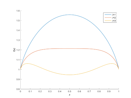
Figure 1: The function $f(x)$ corresponding to the Ising model for $\alpha=0$ and $\beta=1,2,3$, blue, red and yellow respectively

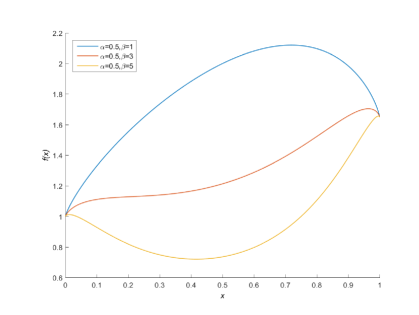
Figure 2: The function $f(x)$ corresponding to the Ising model for $\alpha=0.5$ and $\beta=1,3,5$, blue, red and yellow respectively

Since we have good control over $f$ in this case, we can, to get some numbers, upper bound the constants needed in the $O(n^{2})$ mixing time bounds, using the bounds derived. Of course these are very likely to overestimate what is required in practice by orders of magnitude. We have done the calculations for $(\alpha,\beta)=(0,3)$ and $(\alpha,\beta)=(0.5,5)$. In the first case it turns out that in order to get total variation of at most $0.1$, $K=53$ suffices and the runtime of the algorithm becomes at most $21400n^{2}$. If we instead go for total variation of at most $0.01$, $K=80$ is sufficient and the runtime is bounded by $6.1\cdot 10^{6}n^{2}$.

For the second case the corresponding numbers are $K=11.7$ and $7.3\cdot 10^{6}n^{2}$ for total variation of $0.1$ and $K=17.6$ and $2.3\cdot 10^{9}n^{2}$ for total variation of $0.01$.

Experiments. We have also run some experiments in Matlab for the case $(\alpha,\beta)=(0.5,5)$ and $n=100$. Inspection of $f$ shows that aiming for a total variation distance at most $0.01$, the mixing time starting from $0$ is of order $10^{14}$ and a sample of size $100$ would take order $10^{16}$ time steps. We follow the advice from Remarks (iii) and (v) and try $K$ larger and larger until satisfactory performance is achieved. We choose $K=2,4,6,\ldots$ and for each $K$ we collect a sample of size $100$. With considerable margin we have $b:=(\max_{x}f(x))/(\min_{x}f(x))<1.6$. By Theorem 1.5, the mixing time on $B_{K}$ when governed by $f^{K}$ is or order $O(K^{3}b^{K})$ and we speculate that $K^{2}b^{K}$ steps is sufficient. We then finish off by running $O(n\log n)$ steps on $B_{n}$ governed by $f^{n}$; we guess that $n\log n$ suffices. So, in summary, we run random walk starting from $0$ on $B_{K}$ governed by $f^{K}$ for $K^{2}1.6^{K}$ steps and then continue for another $n\log n$ steps on $B_{n}$ and then collect a sample point. This is repeated $100$ times for the desired sample size.

It turns out that $K=12$ is quite sufficient and if we settle for total variation of $0.05$, $K=8$ seems more than enough. The total number of steps required for running the procedure up to $K=k$ is $100(\sum_{j\in\{2,4,\ldots,k\}}j^{2}1.6^{j}+100\log(100))$ which for $k=12$ is approximately $5.5\cdot 10^{6}$ and takes less than a minute and for $k=8$ is approximately $3.9\cdot 10^{5}$ steps and takes only seconds. We also tried (the hopeless task of) running directly on ${}^{B}_{n}$ governed by $f_{n}$. Collecting a sample of size $100$, running for each sample point $10^{7}$ time steps takes about three hours and is nowhere near to escape from the lower mode at any run.

In Figure 3, we have plotted histograms of the results for $K=2,4,6,8,10,12$ together with the correct probability mass function in orange.

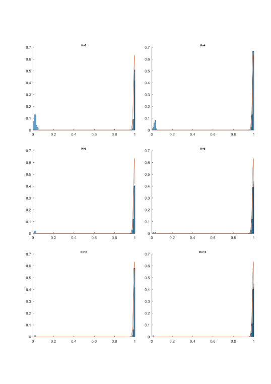
Figure 3: Samples of simulated annealing in the Ising model with $K=2,4,6,8,10,12$.

The mean-field Ising model is a special case of the mean-field $q$-state Potts model. The state space is $\{1,2,\ldots,q\}^{n}$ and the probability distribution is given by

$$\mu^{n}(u)\propto\exp\left(\sum_{i=1}^{q}\alpha_{i}k_{i}(u)-\frac{1}{n}\sum_{1\leq i<j\leq q}\beta_{ij}k_{i}(u)k_{j}(u)\right),$$

where $k_{i}(u)=|\{r:u_{r}=i\}|$ and $\alpha_{i}$, $i=1,\ldots,q$ and $\beta_{ij}$, $1\leq i<j\leq q$ are nonnegative parameters. This measure is invariant under permutations and the projection onto the equivalence classes of vertices with the same spin is indistinguishable from

$$\pi^{n}(x)=f(x)^{n},$$

for $x$ in the $q-1$-dimensional simplex $\{z=(z_{1},\ldots,z_{q-1})\in B_{n}^{q-1}:\sum_{i=1}^{q-1}z_{i}\leq 1\}$, where

$$f(x)=\frac{1}{\prod_{i=1}^{q}x_{i}^{x_{i}}}\exp\left(\sum_{i=1}^{q}\alpha x_{i}-\sum_{1\leq i<j\leq q}\beta_{ij}x_{i}x_{j}\right)$$

and where $x_{q}=\sum_{i=1}^{q-1}x_{i}$. Theorem 1.5 applies.

$\Box$

Example. Latent Dirichlet Allocation. Latent Dirichlet Allocation (LDA) is a model used to latent topics in documents. It was introduced in Blei et. al. [3] and has reached an almost iconic status in the family of probabilistic models for textual data and many variants have been developed since.

A large corpus of documents is to be classified into topics and we want to determine for each word in each document which topic it comes from. Knowing this we can also classify the documents according to the proportion of words of the different topics it contains. LDA is a generative Bayesian model and the setup is that one has a fixed number $D$ of documents of lengths $N_{d}$ a fixed set of topics $t_{1},t_{2},\ldots,t_{K}$ and a vocabulary that consists of a fixed set of word types (i.e. distinct words that appear somewhere in the corpus) $w_{1},w_{2},\ldots,w_{V}$. These are specified in advance. The number of topics is usually not large, whereas the number of words in the vocabulary is. Next, for each document $d=1,\ldots,D$, a multinomial distribution $\theta_{d}=(\theta_{d}(1),\ldots,\theta_{d}(K))$ over topics is chosen according to a Dirichlet prior with a known parameter $\alpha=(\alpha_{1},\ldots,\alpha_{K})$. For each topic $t$ a multinomial distribution $\phi_{t}=(\phi_{t}(1),\ldots,\phi_{t}(V))$ according to a Dirichlet prior with parameter $\beta=(\beta_{1},\ldots,\beta_{V})$ independently of each other and of the $\theta_{d}$:s. Given these, the corpus is then generated by for each position (or token) $j=1,\ldots,N_{d}$ in each document $d$, picking a topic $z_{dj}$ according to $\theta_{d}$ and then picking the word token at that position according to $\phi_{z_{dj}}$, doing this independently for all positions. (So the LDA is a so called ”bag of words” model, i.e. it is invariant under permutations within each document.)

Given the corpus, $\mathbf{W},$ i.e. all the observed words, we want to make inference about the latent quantities: the latent topics $z_{dj}$ and the multinomial parameters $\theta_{d}$, $d=1,\ldots,D$ and $\phi_{t}$, $t=1,\ldots,K$. Since the model is Bayesian, this means that we want to sample from the posterior distribution over these quantities. One standard method is collapsed Gibbs sampling of the $z_{dj}$:s; integrating over (i.e. collapsing) the $\theta$:s and the $\phi$:s, the marginal distribution over the $z_{dj}$:s is straightforward to compute. In particular the conditional distribution of the topic at a given token given the topics at all other tokens, has a simple expression. This allows for Gibbs sampling; at each time step pick a token at random and update according to the conditional distribution of the topic there.

Let us consider the case $K=2$. (In practice $K$ will be larger of course, e.g. $K=50$ or $K=100$ are common choices, but we expect that the essentials on mixing of the Gibbs sampler are captured by this simple special case.) For $\alpha\equiv 1$, $\beta\equiv 1$, the marginal distribution on the topics has a simple closed form expression:

$$\mu(z)\propto\frac{\binom{n_{..}+2V-2}{k_{..}+V-1}}{\prod_{d=1}^{D}\binom{n_{d.}}{k_{d.}}\,\prod_{j=1}^{V}\binom{n_{.j}}{k_{.j}}},$$

$z\in\{1,2\}^{n_{..}}$. Here $n_{dj}$ is the number of tokens with word $j$ in document $d$ and $k_{dj}$ is the number of these tokens that are assigned topic $1$. The dot-notations refer to summing over the dotted index, e.g. $k_{.j}=\sum_{d=1}^{D}k_{dj}$ is the total number of times that an instance of word $j$ has been assigned topic $1$. Note that $n_{d.}=N_{d}$ and hence $n_{..}$ is the total number of tokens in the corpus. For convenience, drop the dots at $n_{..}$ and write just $n$ for the total number of tokens.

The distribution is invariant under permutations of topic assignments within the occurrences of a given word in a given document and the projection of $\mu$ on the resulting equivalence classes is

$$\nu(k)\propto\frac{\binom{n+2V-2}{k_{..}+V-1}\prod_{d=1}^{D}\prod_{j=1}^{V}\binom{n_{dj}}{k_{dj}}}{\prod_{d=1}^{D}\binom{n_{d.}}{k_{d.}}\,\prod_{j=1}^{v}\binom{n_{.j}}{k_{.j}}},$$

$k=(k_{11},\ldots,k_{DV})\in[n_{11}]\times...\times[n_{DV}]$.

For this to fit nicely into the framework of this paper, we consider the asymptotics as the number of documents $D$ is kept fixed and $n\rightarrow\infty$ in such a way that $n_{dj}/n=c_{dj}$ for $c_{dj}\geq 0$, $d=1,\ldots,D$, $j=1,\ldots,V$. Let $h(x)=(x^{x}(1-x)^{1-x})^{-1}$, $x\in[0,1]$. Let $x_{dj}=k_{dj}/n$, let $S=[0,c_{11}]\times\ldots\times[0,c_{DV}]$ and let $f:S\rightarrow(0,\infty)$ be given by

$$f(x)=\frac{h(x_{..})\prod_{d=1}^{D}\prod_{j=1}^{V}h(x_{ij}/c_{dj})^{c_{dj}}}{\prod_{d=1}^{D}h(x_{d.}/c_{d.})^{c_{d.}}\prod_{j=1}^{V}h(x_{.j}/c_{.j})^{c_{.j}}}.$$

Let $\pi$ be the probability measure on $B:=S\cap B_{n}^{DV}$ given by

$$\pi(x)\propto f(x)^{n}.$$

Then rewriting $\nu$ as a measure on $B$, $\nu$ and $\pi$ are asymptotically indistinguishable in the sense that the total variation distance between them vanishes (very quickly) as $n\rightarrow\infty$. which means that a sample from one works as a substitute for the other.

Hence Gibbs sampling for LDA exhibits exponential mixing time if $f$ has more than one local maximum. It is not obvious from a look at $f$ if this is the case or not. In [10], we studied the special case $D=3$, $V=3$, $n_{d.}=m$ for all $d$, $c_{11}=9/30$, $\alpha_{12}=1/30$, $c=1/3$, $c=1/3$ and $c_{dj}=0$ for the other $(d,j)$:s. It turned out that local maxima can be found when $(x_{11},x_{12},x_{22},x_{33})$ equals $(9/30,1/30,1/3,0)$, $(9/30,0,0,1/3)$ or $(0,1/30,1/3,1/3)$ (and the corresponding three points given by swapping the topics); this phenomenon occurs since the model forces a classification into two topics, when there is really three topics in the text. The first of these is the uniquely largest and hence the posterior puts asymptotically almost all of its mass close to that point. Figure 4 illustrates this partially by plotting $f(x_{11},1/30,1/3,x_{33})$, which has local maxima at the points $(x_{11},x_{33})=(0,0)$, $(3/10,0)$ and $(0,1/3)$, i.e. the points where no words, all instances of word 1 or all instances of word 3 are classified as belonging to the same topic as all instances of word 2.

Figure 4: The function $f(x_{11},1/30,1/3,x_{22})$

This is an example of a situation that fits into the framework, but where the local maxima are on the boundary of the domain of the state space of the MCMC.

Remark. We believe that whenever a corpus is of a form that is ”typical” outcome of a corpus generated by LDA with $L\leq K$ topics and then classified with $K$ topics, $f$ does not have a finite number of isolated local maxima and that Gibbs sampling mixes rapidly. The case $D=2$, $V=2$, $(c_{11},c_{12},c_{21},c_{22})=(3/20,7/20,3/10,1/5)$ was considered in [11] and we found that $f$ is maximized on a whole two-dimensional surface cutting through the four-dimensional domain and that mixing happens in $O(n^{2})$ steps.

Experiments. We ran our SA strategy on some different corpora, to see how well the basic SA idea works in the very simplified example just described as well as on a few more realistic corpora. What we did was not exactly the SA technique described in this paper, but intuitively very close. For posterior sampling for LDA in its general form, see [GS], the updated position $(d,j)$ is given topic $k$ with probability proportional to

$$\rho(k):=\frac{(\alpha+\ell_{d}(k))(\beta+m_{k}(v_{dj}))}{V\beta+m_{k}},$$

where $\ell_{d}(k)$ is the number of tokens in document $d$ that are assigned topic $k$, $m_{k}(v)$ is the number of positions in the corpus that are assigned topic $k$ and word $v$, $m_{k}=\sum_{v}m_{k}(v)$ is the total number of tokens assigned topic $k$ and $V$ is the size of the vocabulary. All quantities are counted with position $(d,j)$ excluded. This updating rule corresponds to standard Gibbs sampling for the Ising model in the example above. In this general formulation, there is no natural projection onto a space of the form $B_{n}^{d}$, so the natural way to sample according to the SA idea is to sample according to $\rho(k)^{\kappa/n}$ for some $\kappa=\Theta(1)$ for $O(n^{2})$ steps and then for a short time with $\kappa=n$. Write $\sigma=\kappa/n$.

Now, for computational reasons, it is undesirable to use a factor e.g. of the form $(\alpha+\ell_{d}(k))^{\sigma}$. Then we use that since $\ell_{d}(k)$ is typically much smaller than $n$, a Taylor approximation gives that $(\alpha+\ell_{d}(k))^{\sigma}$ is very close to $1+\tau\ell_{d}(k)/\alpha\propto\alpha+\sigma\ell_{d}(k)$. Using this and the analogous approximations of the other factors, we are not far off if we update so that the chosen position $(d,j)$ is assigned topic $k$ with probability proportional to

$$\tilde{\rho}(k;\sigma)=\frac{(\alpha+\sigma\ell_{d}(k))(\beta+\sigma m_{k}(v_{dj}))}{V\beta+\sigma m_{k}}.$$

Observe that taking $\sigma=1$ gives $\rho=\tilde{\rho}$. The experiments were run with these updating probabilities.

The first example was the situation described above, i.e. the corpus consisted of three documents of length $n_{i.}$ each, consisting of $9/10$ of word 1 and $1/10$ of word 2 in the first document and then two documents consisting of all $2$:s and all $3$:s respectively. The hyperparameters were $\alpha=\beta=1$. We will refer to this corpus as the toy corpus.

We first checked the behavior of standard collapsed Gibbs sampling without SA, started from a state uniformly chosen over the $2^{n}$ topic assignments (where $n=n_{..}$), to see how often it ended up in each of the three modes. The experiment was run $1000$ times with $n_{..}=1200$. Figure 5 shows a histogram over three modes where these are characterized by their respective log posterior density. We find that the problem of multimodality is real and that the mode that we most frequently end up in is in fact the worst one.

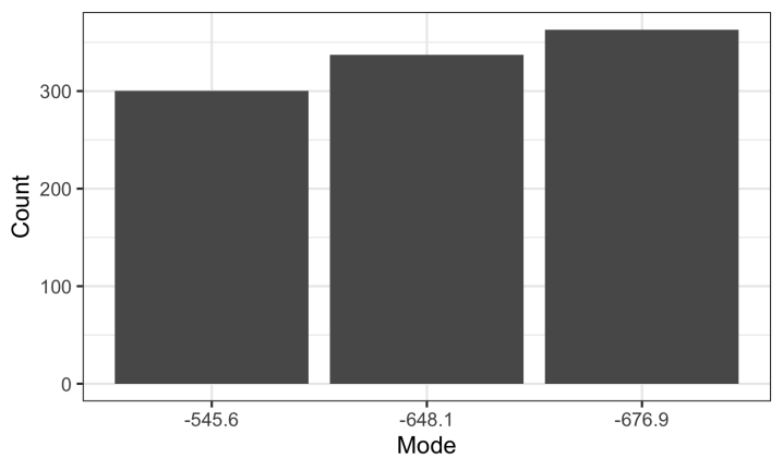
Figure 5: Histogram over the modes (as log posterior density) for collapsed Gibbs sampling on the toy corpus started from uniformly random topic configuration.

For SA, we made $500$ runs each for $\kappa=1,2,4,8,16,32,64,128$ for $5n^{2}$ time steps. Each run was finished with $\kappa=n$ for $n^{2}$ steps. Each run was started in the second best mode of $f$. Figure 6 shows, for each $\kappa$, a histogram over what modes the annealed collapsed Gibbs ended in. Note that for $\kappa\leq 4$, the fitness landscape has been made too flat and the results are indistinguishable from standard Gibbs with uniform start. For $\kappa\geq 32$, the opposite happens and the sampler is stuck in the starting mode. For $\kappa=8,16$, the desired behavior occurs and the sampler finds the optimal mode virtually all the time.

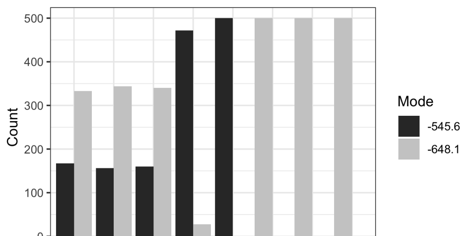
Figure 6: Simulated annealing for collapsed Gibbs sampling on toy corpus.

We further studied the behavior on real data; we created small corpora made up of three different translations (English, Swedish and French) of the novel Three men and a boat by Jerome K. Jerome. We set up the corpus by first removing common stopwords from each language (such as a, the, etc. ). Then, we extracted the first words of each chapter until we fulfilled two criteria; first that each word should occur ten or more times and second that the total number of tokens should be so that 80% of the words were in English and 10% in Swedish and French, respectively. In total, the corpus was made up of 4999 word tokens (3963 English, 531 French, and 505 Swedish word tokens).

Using these words, we created three corpora with different document definitions.

1. Corpus 1: We combined Ch. 1-10 and 11-19 per language. Hence we have got document: two English, two French, and two Swedish.

2. Corpus 2: As in Corpus 1, but the English tokens were instead split up into documents that each covered two chapters. Hence, this corpus had fourteen documents: ten English, two French, and two Swedish.

3. Corpus 3: As in Corpus 1, but the English tokens were divided into five documents covering four chapters each. Hence, this corpus had nine documents: five English, two French, and two Swedish.

These experiments were run with $K=3$ and 100 runs for each value of $\kappa$. The hyperparameter values were again $\alpha=\beta=1$. In each case, the best mode in terms of posterior probability was to classify all English documents as one topic, all French documents as another topic and all Swedish documents as a third topic. There were other modes however, and our runs were started in the second best mode, which was to consider the French and Swedish documents together as one topic and the third topic empty.

In Figure 7, we find the results on Corpus 1. One can read out that there is a range of $\kappa$ values around $128$, where almost all runs end up in the best mode. For smaller $\kappa$, the behavior is like standard Gibbs sampling started from a uniformly random configuration and for larger $\kappa$ we get stuck in the starting mode.

The results on Corpus 2 are found in Figure 8. One can read out that some small and bordering on significant improvement over standard Gibbs started from uniformity was achieved for $\kappa=32,64$. In order to check if this improvement was a random phenomenon, we performed a refined search for higher values of $\kappa$ without finding further improvement.

In Figure 9, the results for Corpus 3 are found. Here a clear and significant improvement is found for $\kappa$ between 150 and 180. This result is not as pronounced as for Corpus 1 but a lot more than for Corpus 2, which was intuitively anticipated, since Corpus 3 is ”in between” Corpus 1 and Corpus 2.

It is not clear to us why dividing the English text into a larger number of documents seems to harm the performance of SA and it would be interesting to understand that, something we leave for future work.

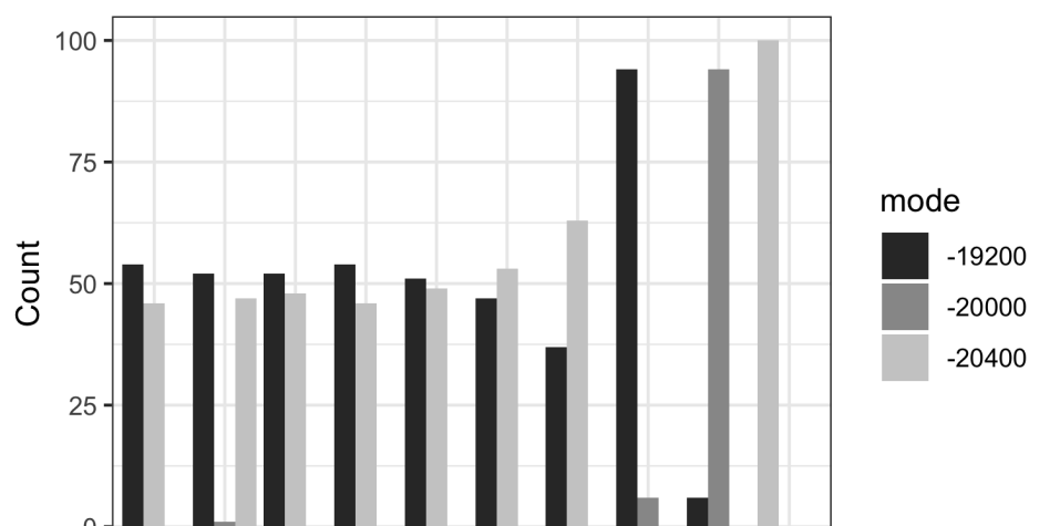
Figure 7: Simulated annealing for collapsed Gibbs sampling on Corpus 1.

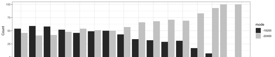
Figure 8: Simulated annealing for collapsed Gibbs sampling on Corpus 2.

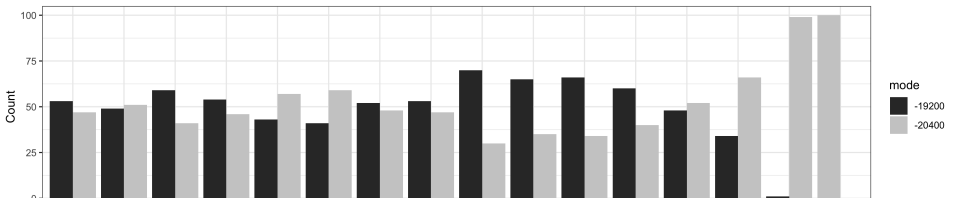
Figure 9: Simulated annealing for collapsed Gibbs sampling on Corpus 3.

$\Box$

Example. 3S1 phase shifts from an analysis of neutron-proton scattering cross sections. I am grateful to Christian Forssén and Andreas Ekström who provided the data in this example.

Bayesian analysis methods are increasingly being used in theoretical nuclear physics [17]. A specific example is the determination of parameters in a chiral effective field theory description of the low-energy, strong interaction between neutrons and protons (see e.g. [4], [9], [13], and references therein). In short, we seek to find the parameter vector $\theta$ that minimizes the deviation between the model and experimental data. In this specific case, the calibration data corresponds to the 3S1 phase shifts from an analysis of neutron-proton scattering cross sections [16]). See, e.g. [17] for more details on the definition of the likelihood function.

In this example a Bayesian model of the standard form with two parameters,

$$g(\theta_{0},\theta_{2})\propto L(y;\theta_{0},\theta_{1})q(\theta_{0},\theta_{1}),$$

is given, where the prior $q$ is independent $N(0,5)$, i.e.

$$\log q(\theta_{0},\theta_{1})=\frac{1}{10}(\theta_{0}^{2}+\theta_{1}^{2}),$$

and $L$ is an intractable likelihood of the form

$$\log L(y;\theta_{0},\theta_{1})=\sum_{i=1}^{n}\left(\frac{y_{i}-h(x_{i},\theta_{0},\theta_{1})}{\sigma_{i}}\right)^{2}.$$

Here $h$ is some intractable function and $x_{i}$ is a set of covariates for observation $y_{i}$.

Experiments: Data consisted of $\log g$ computed on a $300\times 300$ grid together with a warning that $\log g$ may look ”very odd”, but that it certainly has some pronounced peaks. Hence it seemed prudent to act according to remarks (vi) and (vii). We collected a sample, $S$, of $10^{5}$ points of the domain and took $M$ to be the 1000’the largest value of $\log g$ on $S$ and replaced $\log g$ with $\max(\log g,M)$. Next, we observed that $\max_{u,v\in S}(\log g(u)-\log g(v))\approx 1.86\cdot 10^{5}$. This means that $\max_{u}(g(u)/g(v))$ with the maximum taken over the whole domain is at least $e^{186000}$. We hoped that the true value is not significantly larger than that and took $f=g^{1/(4\cdot 186000)}$ and then hoped that the ratio of the max and min of $f$ is approximately $e^{1/4}$. (Computations are of course made at log-scale.)

The relaxation time for ordinary lazy random walk on $B_{n}^{2}$ is $4n^{2}$, so we hoped that for sufficient mixing of random walk governed by $f^{K}$ on $B_{N}^{2}$, $4N^{2}e^{K/4}$ steps is enough. We then finished off by $n\log n$ steps on $B_{n}^{2}$ according to $g$. We tried running with $N=K$ and the values of $K$ that were tried are $5,10,15,20,30,40$. For each $K$ we collected a sample of size $100$. This took 12 hrs to run through with Matlab. The result of this first attempt was disappointing as no zooming in on any region could be seen.

One possible explanation for this could be that peaks are so thin that the $N$:s are simply so small that the peaks vanish on the course grids that they correspond to, so in the next attempt, we tried to fix $N=100$ (and not $300$ as we considered the problem to be too misbehaved if peaks are of no more than two pixels wide). We ran $K=5,10,15,20$ and found that in this case, the algorithm indeed starts to zoom in. In Figure 10, histograms of the samples are given.

In this example, we of course in fact have complete control of $g$, but on larger grids in higher dimensions (say on $B_{1000}^{4}$), this would not be the case and we have worked as if we were in that situation. In Figure 11, we have plotted $\log g$ (with the floor at $M$), from an ordinary view and from a birds perspective. The latter reveals that peaks are indeed very thin.

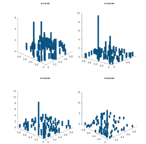
Figure 10: Samples for the 3S1 phase shifts example.

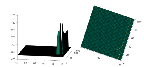
Figure 11: The log posterior (with floor) for the 3S1 phase shifts example. The bird’s view on the right hand side reveals that the peaks are very thin.

$\Box$

Acknowledgment. We are very grateful to nuclear physicists Christian Forssén and Andreas Ekström at Chalmers whose inspiration was the spark that set off this work and who provided me with data for the 3S1 phase shifts example above.

References

- [1] D. Aldous and J. A. Fill, Reversible Markov Chains and Random Walks on Graphs, Unfinished monograph at http://www.stat.berkeley.edu/ aldous/RWG/book.html
- [2] N. Bhatnagar and D. Randall (2004), Torpid mixing of simulated tempering on the Potts model, Proceedings of the 15th ACM-SIAM Symposium on Discrete Algorithms.
- [3] D. M. Blei, A. Y. Ng and M. I. Jordan (2003), Latent Dirichlet Allocation, Journal of Machine Learning Research 93, 993-1022.
- [4] B. D. Carlsson, A. Ekström, C. Forssén, D. Fahlin Strömberg, G. R. Jansen, O. Lilja, M. Lindby, B. A. Mattsson, and K. A. Wendt (2016), Uncertainty Analysis and Order-by-Order Optimization of Chiral Nuclear Interactions, Physical Review X 6(1):011019–23, February 2016.
- [5] G. Chen and L. Saloff-Coste (2013), On the mixing time and spectral gap for birth and death chains, ALEA Lat. Am. J. Probab. Math. Stat. 10, 293–321.
- [6] P. Diaconis and L. Saloff-Coste (1993), Comparison theorems for reversible Markov chains, Ann. Appl. Probab. 3, 696-730.
- [7] P. G. Doyle and J. L. Snell, Random Walks and Electric Networks, Carus Mathematical Monographs, 1984. See also https://math.dartmouth.edu/ doyle/docs/walks/walks.pdf.
- [8] T. Duong-Ba, T. Nguyen and B. Bose (2014), Convergence rate of MCMC and simulated annealing with applications to client-server assignment problem (2014), Stochastic Analysis Appl..
- [9] E. Epelbaum, H.-W. Hammer, and Ulf-G. Meißner (2009), Modern theory of nuclear forces, Rev. Mod. Phys. 81, 1773–1825, December 2009.
- [10] J. Jonasson (2017), Slow mixing for Latent Dirichlet Allocation, Statist. Probab. Letters 129, 96-100. Corrigendum at http://www.math.chalmers.se/homepages/jonasson/LDAmixing_correction.pdf.
- [11] J. Jonasson (2017), Fast mixing for Latent Dirichlet Allocation, Preprint ArXiv https://arxiv.org/abs/1701.02960.
- [12] D. A. Levin, M. Luczak and Y. Peres (2010), Glauber dynamics for the Mean-field IsingModel: cut-off, critical power law and metastability, Probab. Th. Rel. Fields 146, 223-265.
- [13] R. Machleidt and D. R. Entem (2010), Chiral effective field theory and nuclear forces, Physics Reports- Review Section Of Physics Letters 503(1), 1–70.
- [14] B. Morris and Y. Peres (2005), Evolving sets, mixing and heat kernel bounds, Probability Theory and Related Fields 133, 245-266.
- [15] N. Madras and Z. Zheng (2003), On the swapping algorithm, Random Struct. Algorithms 22, 66-97.
- [16] V. G. J. Stoks, R. A. M. Klomp, M. C. M. Rentmeester and J. J. de Swart (1993), Partial-wave analysis of all nucleon-nucleon scattering data below 350 mev, Phys. Rev. C 48, 792–815, August 1993.
- [17] S. Wesolowski, R. J. Furnstahl, J. A. Melendex and D. R. Phillips (2018), Exploring Bayesian parameter estimation for chiral effective field theory using nucleon-nucleon phase shifts, J. of Physics G: Nuclear and Particle Physics 2018, to appear. Doi: https://iopscience.iop.org/article/10.1088/1361-6471/aaf5fc
- [18] D. B. Woodard, S. S. Schmidler and M. Huber (2009), Conditions for rapid mixing of parallel and simulated tempering on multimodal distributions, Ann. Appl. Probab 19, 617-640.