Middle aged $\gamma$-ray pulsar J1957+5033 in X-rays: pulsations, thermal emission and nebula

Abstract

We analyze new XMM-Newton and archival Chandra observations of the middle-aged $\gamma$-ray radio-quiet pulsar J1957+5033. We detect, for the first time, X-ray pulsations with the pulsar spin period of the point-like source coinciding by position with the pulsar. This confirms the pulsar nature of the source. In the 0.15–0.5 keV band, there is a single pulse per period and the pulsed fraction is $\approx 18\pm 6$ per cent. In this band, the pulsar spectrum is dominated by a thermal emission component that likely comes from the entire surface of the neutron star, while at higher energies ($\gtrsim 0.7$ keV) it is described by a power law with the photon index $\Gamma\approx 1.6$. We construct new hydrogen atmosphere models for neutron stars with dipole magnetic fields and non-uniform surface temperature distributions with relatively low effective temperatures. We use them in the spectral analysis and derive the pulsar average effective temperature of $\approx(2-3)\times 10^{5}$ K. This makes J1957+5033 the coldest among all known thermally emitting neutron stars with ages below 1 Myr. Using the interstellar extinction–distance relation, we constrain the distance to the pulsar in the range of 0.1–1 kpc. We compare the obtained X-ray thermal luminosity with those for other neutron stars and various neutron star cooling models and set some constraints on latter. We observe a faint trail-like feature, elongated $\sim 8$ arcmin from J1957+5033. Its spectrum can be described by a power law with a photon index $\Gamma=1.9\pm 0.5$ suggesting that it is likely a pulsar wind nebula powered by J1957+5033.

1 Introduction

Neutron stars (NSs) are born in supernova explosions at very high temperatures $\sim 10^{11}$ K (e.g. Müller, 2020, and references therein). They lose the initial thermal energy via neutrino emission from their interiors and then via photon emission from their surfaces (e.g. Yakovlev & Pethick, 2004, and references therein). The cooling rate is sensitive to the physical properties of the superdense matter inside NSs, which are still poorly known (e.g. Yakovlev et al., 2005). The equation of state (EoS) of such matter can be constrained by comparison of cooling theories with NSs surface temperatures derived from observational data.

The middle-aged PSR J1957+5033 (hereafter J1957) is a radio-quiet $\gamma$-ray pulsar discovered with the Fermi Large Area Telescope (LAT) (Saz Parkinson et al., 2010). Its spin period $P=375$ ms and period derivative $\dot{P}=7.1\times 10^{-15}$ s s^-1 imply the characteristic age $t_{\mathrm{c}}\equiv P/2\dot{P}\approx 840$ kyr, the spin-down luminosity $\dot{E}=5.3\times 10^{33}$ erg s^-1 and the characteristic (spin-down) magnetic field $B=1.65\times 10^{12}$ G. The distance to the pulsar is poorly known. The only available estimate, 0.8 kpc, is the so-called ‘pseudo-distance’ obtained using empirical correlation between the distance and the $\gamma$-ray flux above 100 MeV (Abdo et al., 2013). It is known to be uncertain by a factor of 2–3. Analysing the $\gamma$-ray pulse profile, Pierbattista et al. (2015) estimated the magnetic inclination and line of sight angles of J1957 for different $\gamma$-ray emission geometries.

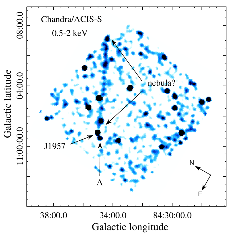
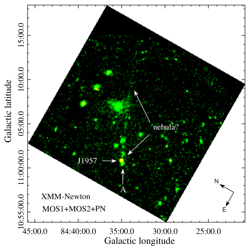
Figure 1: Images of the J1957 field. Left: Chandra ACIS-S3 chip field-of-view in the 0.5–2 keV band. Right: 18 arcmin $\times$ 18 arcmin XMM-Newton combined MOS1+MOS2+PN image (red = 0.2–0.5 keV, green = 0.5–2 keV). J1957, the nearby star ‘A’ and the presumed trail-like nebula are marked. Compasses correspond to the equatorial coordinate system.

The pulsar X-ray counterpart was identified by position in the 25-ks Chandra Advanced CCD Imaging Spectrometer (ACIS-S) observation (Marelli et al., 2015). Its spectrum in the 0.3–10 keV band was found to be well described by the absorbed single power-law (PL) with a photon index $\Gamma=2.1\pm 0.3$, an energy integrated unabsorbed flux $F_{X}=(3.0\pm 0.5)\times 10^{-14}$ erg s^-1 cm^-2 and an absorption column density $N_{\mathrm{H}}$ $<2.5\times 10^{20}$ cm^-2 (Marelli et al., 2015).

We reanalyzed the Chandra data and confirmed the results by Marelli et al. (2015). However, we found an unexpectedly large count number in the 0.1–0.3 keV band – 30 against 90 counts detected in the 0.3–10 keV band. This indicates the presence of a second soft component in the pulsar spectrum likely related to the thermal emission from the surface of the NS with a very low effective temperature. In this case, J1957 becomes especially interesting for comparison with NS cooling theories according to which at its characteristic age the pulsar should have already passed from a relatively slow neutrino cooling stage to a significantly faster photon stage where observational data on thermal emission from cooling NSs are particularly scarce. Unfortunately, the soft component cannot be confirmed using the Chandra data since the ACIS energy scale is not calibrated below 0.3 keV. 3.2 s time resolution of the observations does not also allow to detect pulsations with the pulsar period. Therefore, we performed dedicated XMM-Newton observations of J1957. Here we present the analysis of these data. The X-ray data are described in Section 2. Timing and spectral analysis of J1957 are presented in Sections 3 and 4. The results are discussed in Section 5 and summarized in Section 6. Some details of the analysis are given in the Appendices.

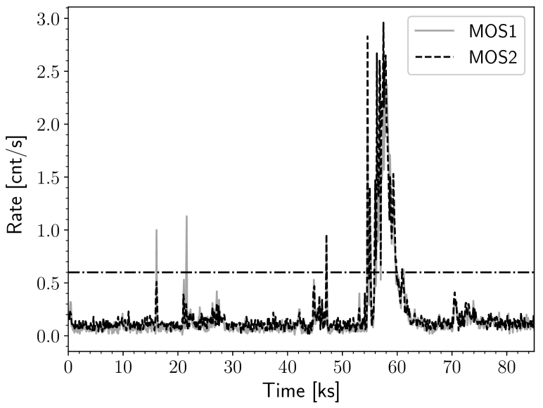
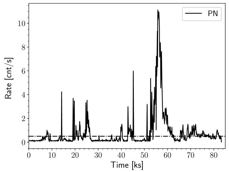
Figure 2: High-energy light curves obtained from the FOVs of MOS (10–12 keV; left) and pn (12–14 keV; right) detectors. Dash-dotted lines indicate thresholds used to filter out periods of background flares.

2 X-ray data and imaging

The J1957 field was observed with XMM-Newton on 2019 October 5 (ObsID 0844930101, PI D. Zyuzin). The total exposure was about 87 ks. The European Photon Imaging Camera Metal Oxide Semiconductor (EPIC-MOS) detectors were operated in the full-frame mode with the imaging area of about 28 arcmin $\times$ 28 arcmin and the medium filter and the EPIC-pn camera – in the large window mode with the imaging area of about 13.5 arcmin $\times$ 26 arcmin and the thin filter. We also used the Chandra/ACIS-S archival dataset (ObsID 14828) where the pulsar was exposed on the S3 chip. To analyze the data, we utilized the XMM-Newton Science Analysis Software (xmm-sas) v. 17.0.0 and Chandra Interactive Analysis of Observations (ciao) v. 4.12 packages.

The Chandra dataset was reprocessed using the chandra_repro tool. Applying the fluximage task, we created the exposure-corrected image of the ACIS-S3 chip which is presented in the left panel of Fig. 1 where the pulsar counterpart and the nearby star ‘A’ are marked. The wavdetect command was used to obtain coordinates of point-like sources. For J1957, we derived R.A. = 19^h57^m38$.\!\!^{\mathrm{s}}$390(6) and Dec. = +50^∘33^′21$\aas@@fstack{\prime\prime}$02(5) (numbers in parentheses are 1$\sigma$ pure statistical uncertainties).

We combined the data from both MOS and PN detectors to obtain deeper X-ray images using the ‘images’ script (Willatt & Ehle, 2016). The resulting image is shown in the right panel of Fig. 1. Since XMM-Newton has lower spatial resolution than Chandra, J1957 is somewhat blurred with the star ‘A’. One can see a faint thin feature protruding from J1957 almost perpendicularly to the Galactic plane. It has a clumpy structure and is also visible in the Chandra image where it extends up to the edge of the ACIS-S detector ($\approx 6$ arcmin). In the XMM-Newton image its length seems to be longer, at least up to $\sim$8 arcmin, though its faintness and some blurring with other sources preclude accurate measurements. This maybe a trail-like pulsar wind nebula (PWN) powered by J1957. One can see that the pulsar is indeed a rather soft source while the presumed PWN is produced by harder photons.

For the further analysis, we filtered out the background flares inspecting high-energy light curves extracted from the field-of-views (FoVs) of all EPIC detectors. We chose the following threshold count rates to define good time intervals: 0.5 counts s^-1 for pn and 0.6 counts s^-1 for both MOS cameras (see Fig. 2). The resulting effective exposures are about 79.8, 79.8 and 48.7 ks for the MOS1, MOS2 and pn detectors, respectively. We selected single to quadruple pixel events (pattern $\leq 12$) for the MOS data and single and double pixel events (pattern $\leq 4$) for the pn data.

3 Timing

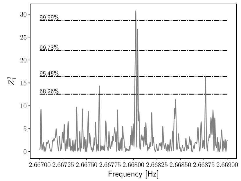
Figure 3: $Z^{2}_{1}$-test periodogram for J1957. Dashed lines show confidence levels.

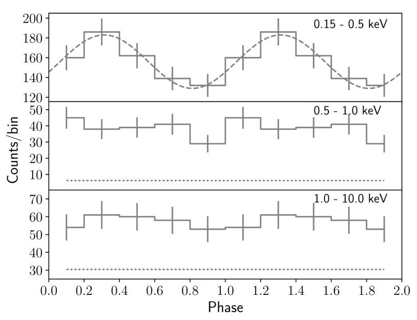
Figure 4: Folded X-ray light curves for J1957 in different energy bands indicated in the panels (periods of background flares are removed). Dotted lines in the middle and bottom panels indicate the background level. In the 0.15–0.5 keV band the background contribution ($\approx 12$ counts phase bin^-1) is very low in comparison with the pulsar count rate and thus it is not shown. The best-fitting sine curve is overlaid.

The timing resolution of the EPIC-pn detector operating in the large window mode is $\approx 48$ ms which allows us to search for pulsations from J1957. We used the event list unfiltered from background flares since multiple time gaps in the data may hamper signal detection. The barycenter correction was applied by the xmm-sas barycen command using DE405 ephemeris and the pulsar coordinates derived from the Chandra data. We extracted events in the 0.15–0.5 keV band using the 12.5-arcsec radius circle around the Chandra position of J1957. Such a small aperture was chosen to eliminate the contribution from the star ‘A’ located at about 20 arcsec from the pulsar. We searched for pulsations utilising $Z^{2}_{1}$-test (Buccheri et al., 1983) and 2.667–2.669 Hz frequency range, encapsulating the predicted pulsar rotation frequency of about 2.6680281 Hz obtained from extrapolation of the Fermi timing solution to the epoch of the XMM-Newton observations (MJD 58761), and with a step of 0.1 $\mu$Hz.

The resulting periodogram is shown in Fig. 3. The maximum $Z^{2}_{1}$ is $\approx$ 30.7. This implies the confidence level of a detection $C=[1-\mathcal{N}\mathrm{exp(-Z^{2}_{1,max}/2)}]\times 100\%=99.996$ per cent (or $\approx 4\sigma$) where $\mathcal{N}=\Delta f\times T_{\mathrm{obs}}$ is the number of statistically independent trials, $\Delta f$ is the frequency range and $T_{\mathrm{obs}}$ is the duration of the observation. The corresponding frequency is 2.6680249(12) Hz (the frequency 1$\sigma$ uncertainty was calculated using the formula from Chang et al. 2012). This is consistent within 3$\sigma$ with the predicted value from Fermi timing solution and firmly establishes the pulsar nature of the X-ray source.

The J1957 X-ray pulse profile obtained using the derived frequency is presented in Fig. 4. We see that pulsations are clearly detected only in the very soft band. Non-detection in harder bands is likely due to the low number of counts from the pulsar. The background-corrected pulsed fraction in the 0.15–0.5 keV band $\mathrm{PF}=(f_{\mathrm{max}}-f_{\mathrm{min}})/(f_{\mathrm{max}}+f_{\mathrm{min}})$, where $f_{\mathrm{max}}$ and $f_{\mathrm{min}}$ are the maximum and minimum intensity of the folded light curve, is $\approx 18\pm 6$ per cent. As an additional check, we fitted the pulse profile in the 0.15–0.5 keV band with a sine function (fundamental component; see Fig. 4) and got the same result. Following the method from Brazier (1994), we estimated the 99 per cent upper limits on the pulsed fraction of $\approx 44$ per cent in the 0.5–1 keV band and $\approx 64$ per cent in the 1–10 keV band.

4 Spectral analysis

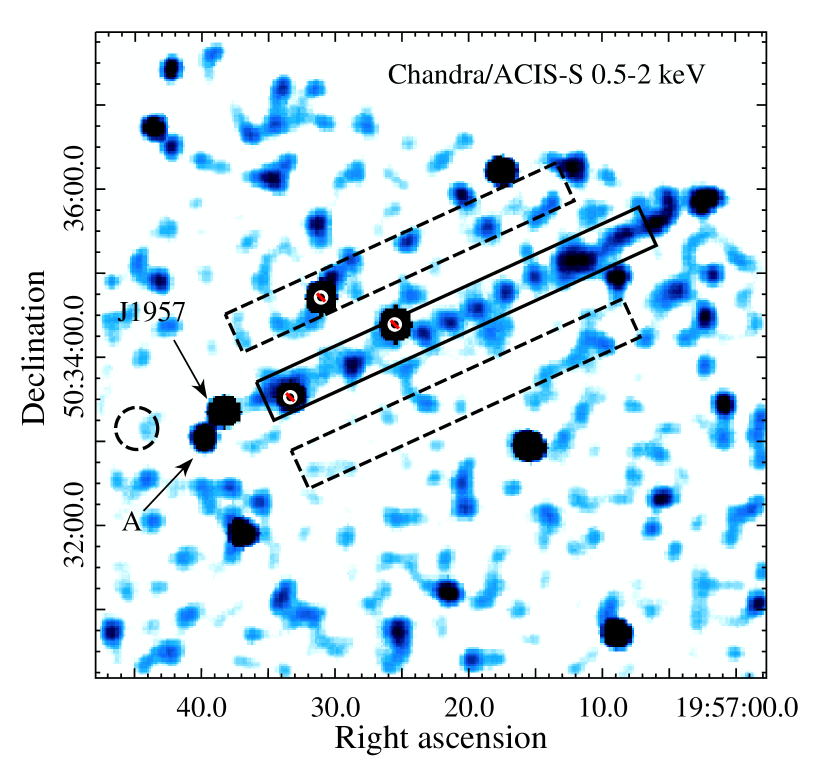
Figure 5: Chandra ACIS image of the J1957 field in the 0.5–2 keV band. J1957 and the nearby star ‘A’ also marked. The background for the pulsar was extracted from the dashed circle. The solid rectangle shows the region used to extract the spectrum of the trail-like nebula while the dashed rectangles were used for the background. Stars excluded from the regions are shown by crossed circles.

4.1 J1957

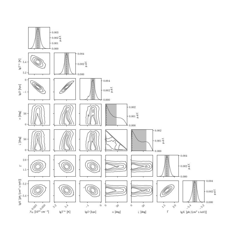
Figure 6: 1D and 2D marginal posterior distribution functions (p.d.f.) for parameters of the nsmdip1$+$PL model (see Table 1). Vertical dashed lines in 1D distributions indicate the best-fitting values while light gray strips show 1$\sigma$ credible intervals. In 2D distributions, 40, 68, 90 and 99 per cent confidence contours are shown.

We extracted the time integrated pulsar spectra from both the XMM-Newton and Chandra data. In the latter case we utilized the specextract routine and the 2.5-arcsec radius aperture. The XMM-Newton spectra were extracted from the 12.5-arcsec radius circle using evselect task and redistribution matrix and ancillary response files were created by rmfgen and arfgen commands. The background spectrum was obtained from the source-free region (see Fig. 5). For the interstellar medium (ISM) absorption, we applied tbabs model with the wilm abundances (Wilms, Allen & McCray, 2000). The spectra were fitted simultaneously in the X-Ray Spectral Fitting Package xspec v.12.10.1 (Arnaud, Gordon & Dorman, 2018). We used the following energy ranges: 0.3–10 keV for the Chandra, 0.2–10 keV for the MOS and 0.15–10 keV for the pn spectra. The resulting number of source counts after background subtraction is 232(MOS1) + 254(MOS2) + 902(pn) + 88(ACIS).

As a first step, to check how different models fit the data, we applied the $\chi^{2}$-statistic and grouped the data to ensure 25 counts per energy bin. The single absorbed PL (which describes the pulsar non-thermal emission of magnetospheric origin) or blackbody (BB, which describes the thermal emission from the NS surface) models resulted in unacceptable fits with reduced $\chi^{2}_{\nu}$ = 2.36 and 5.5 for 54 degrees of freedom (dof), respectively. Then we tried the composite BB + PL model and found that it fits the spectra well with $\chi^{2}_{\nu}$ = 1.13 (52 dof).

For the thermal component, we also tried the NS magnetized atmosphere models nsmaxg (Ho, Potekhin & Chabrier, 2008) presented in the xspec package assuming an NS mass $M_{\mathrm{NS}}$ = 1.4M_⊙ and radius $R=13$ km. However, in this case the temperature tends to the lowest value available for these models $\mathbf{\lg(T/{\rm K})=5.5}$; here and hereafter $\lg\equiv\log_{10}$. Therefore, we calculated another grid of NS atmosphere models, nsmdip, which include lower temperatures for the magnetic fields that seem to be likely for this pulsar. We assumed a dipole magnetic field (taking the effects of General Relativity into account) and a corresponding distribution of the local effective temperature over the stellar surface. In these models, the angle $\alpha$ between the rotation and the magnetic axes and the angle $\zeta$ between the rotation axis and the line of sight can be used as free parameters. The total thermal luminosity $L^{\infty}$ that would be measured by a distant observer is calculated by a proper surface integration and converted into the global effective temperature $T^{\infty}$. The details of calculations are presented in Appendix A.

We have tested several nsmdip models (Table 3). In model nsmdip1, we have assumed the canonical NS mass $M=1.4\mbox{M${}_{\odot}$}$ and magnetic field at the pole $B_{\mathrm{p}}=3\times 10^{12}$ G, which corresponds to the characteristic magnetic field $B\approx 1.65\times 10^{12}$ G of J1957 at the equator derived from the spin-down. The radius $R=12.6$ km was taken according to the EoS BSk24 (Pearson et al., 2018); the corresponding gravitational redshift is $z_{\mathrm{g}}=0.22$, and surface gravity $g_{\mathrm{s}}=1.43\times 10^{14}$ cm s^-2. In order to test a higher redshift, we consider a more compact NS model (nsmdip2) with $M=2\,\mbox{M${}_{\odot}$}$ and $R=11.4$ km ($z_{\mathrm{g}}=0.44$ and $g_{\mathrm{s}}=3\times 10^{14}$ cm s^-2), which approximately corresponds to the EoS BSk26. Model nsmdip3 has the same $z_{\mathrm{g}}$ and $R$ as model 1 but a more consistent magnetic field estimate. The canonical characteristic magnetic field is the equatorial field of an orthogonal rotating dipole in vacuum with the given spin period and its derivative, assuming $R=10$ km and $I_{45}=1$, where $I_{45}$ is the moment of inertia in units of $10^{45}$ g cm² (e.g., Manchester & Taylor 1977). However, according to the EoS BSk24, for $M=1.4\,\mbox{M${}_{\odot}$}$ we have $R=12.6$ km and $I_{45}=1.51$. Moreover, the spin-down of a pulsar is affected by its magnetosphere. Results of numerical simulations of plasma behaviour in the pulsar magnetosphere suggest that the characteristic magnetic field should be multiplied by a factor of $0.8\,(R/\mbox{10 km})^{-3}\,(1+\sin^{2}\alpha)^{-1/2}\,\sqrt{I_{45}}$, where $\alpha$ is the angle between rotational and magnetic axes (Spitkovsky, 2006). For the above-mentioned values of $R$ and $I_{45}$ this implies a 2–3 times weaker field compared to the characteristic one. Thus we adopted $B_{\mathrm{p}}=1.1\times 10^{12}$ G in model nsmdip3 which corresponds to the field strength at the equator $B_{\mathrm{eq}}\approx 6\times 10^{11}$ G, that is 2.7 times smaller than the pulsar characteristic (spin-down) field. We find that all three absorbed nsmdip$+$PL models describe the data equally well as the BB$+$PL model giving $\chi^{2}_{\nu}\approx$ 1.17 (51 dof).

Since the number of source counts is not large, in order to get the most robust estimates of the model parameters and their uncertainties from spectral fits, we regrouped all spectra to ensure at least 1 count per energy bin and therefore used $W$-statistic (Arnaud et al., 2018) which is $C$-statistic (Cash, 1979) suitable for Poisson data with Poisson background. We then performed the fitting using a Markov chain Monte-Carlo (MCMC) sampling procedure. We employed the affine-invariant MCMC sampler developed by Goodman & Weare (2010) and implemented in a python package emcee by Foreman-Mackey et al. (2013). In addition, to estimate the distance to J1957, we used the interstellar absorption–distance relation towards the pulsar as a prior (see Appendix B for details). About 100 walkers and 13000 steps were typically enough to ensure fit convergences. Using the sampled posterior distribution, we obtained the best-fitting parameters of the models with uncertainties, which are defined as their maximal-probability density values and respective credible intervals.

Table 1: Best-fitting parameters for different models with thawed $\alpha$ and $\zeta$ angles and accounting for $\alpha$ + $\zeta$ <= 90^∘.

Model	$N_{\mathrm{H}}$,	$k_{\mathrm{B}}T^{\infty}$,	$R^{\infty}$,	$\lg\,L^{\infty}$,	$\Gamma$	$K$,	$D$,	$-\ln\mathcal{L}$	BIC
	1020 cm-2	eV	km	erg s-1		ph cm-2 s-1 keV-1	pc
BB + PL	$2.2^{+1.6}_{-1.0}$	$54^{+5}_{-7}$	$2.2^{+5.0}_{-2.0}$	$30.66^{+0.85}_{-1.72}$	$1.76^{+0.11}_{-0.11}$	$5.4^{+0.4}_{-0.4}\times 10^{-6}$	$545^{+463}_{-445}$	193.5	416.6
nsmdip1 + PL	$3.6^{+0.6}_{-0.5}$	$21.7^{+2.0}_{-1.7}$	15.4f	$30.83^{+0.16}_{-0.14}$	$1.65^{+0.11}_{-0.10}$	$4.8^{+0.5}_{-0.3}\times 10^{-6}$	$260^{+109}_{-82}$	195.3	432
nsmdip2 + PL	$3.2^{+0.6}_{-0.7}$	$19.8^{+2.0}_{-1.8}$	16.4f	$30.72^{+0.17}_{-0.16}$	$1.66^{+0.10}_{-0.11}$	$4.9^{+0.4}_{-0.4}\times 10^{-6}$	$218^{+164}_{-64}$	195.9	433
nsmdip3 + PL	$2.6^{+0.8}_{-0.5}$	$18.4^{+2.1}_{-2.0}$	15.4f	$30.55^{+0.19}_{-0.21}$	$1.64^{+0.10}_{-0.10}$	$4.9^{+0.3}_{-0.4}\times 10^{-6}$	$210^{+108}_{-106}$	196.1	433.7

• ^† $N_{\mathrm{H}}$ is the absorbing column density, $T^{\infty}=T/(1+z_{\mathrm{g}})$ is the effective temperature as measured by a distant observer, $R^{\infty}=R(1+z_{\mathrm{g}})$ is the radius of the equivalent emitting sphere as seen by a distant observer, $L^{\infty}=L/(1+z_{\mathrm{g}})^{2}=4\pi R^{2}\sigma_{\rm SB}T^{4}/(1+z_{\mathrm{g}})^{2}$ is the bolometric thermal luminosity as measured by a distant observer ($\sigma_{\rm SB}$ is the Stefan-Boltzmann constant), $\Gamma$ is the photon index, $K$ is the PL normalization and $D$ is the distance. For the gravitational redshift $z_{\mathrm{g}}$ and unredshifted radius $R$, see Table 3. The last two columns give the values of the maximum log-likelihood $\ln\mathcal{L}$ and the Bayesian information criterion (BIC). All errors are at 1$\sigma$ credible interval.

• ^f Fixed parameters.

Table 2: The same as in Table 1 but for fixed angles at $\alpha$ = $66^{\circ}$ and $\zeta$ = $24^{\circ}$ ^†.

Model	$N_{\mathrm{H}}$,	$k_{\mathrm{B}}T^{\infty}$,	$R^{\infty}$,	$\lg\,L^{\infty}$,	$\Gamma$	$K$,	$D$,	$-\ln\mathcal{L}$	BIC
	1020 cm-2	eV	km	erg s-1		ph cm-2 s-1 keV-1	pc
nsmdip1 + PL	$3.5^{+0.7}_{-0.6}$	$21.9^{+1.9}_{-1.1}$	15.4f	$30.85^{+0.14}_{-0.09}$	$1.66^{+0.10}_{-0.11}$	$4.9^{+0.4}_{-0.4}\times 10^{-6}$	$263^{+112}_{-78}$	195.1	419.8
nsmdip2 + PL	$3.3^{+0.6}_{-0.8}$	$20.3^{+2.0}_{-1.5}$	16.4f	$30.77^{+0.16}_{-0.14}$	$1.64^{+0.11}_{-0.09}$	$5.0^{+0.3}_{-0.5}\times 10^{-6}$	$224^{+165}_{-63}$	195.7	421.0
nsmdip3 + PL	$2.9^{+0.5}_{-0.7}$	$19.8^{+1.5}_{-2.6}$	15.4f	$30.67^{+0.13}_{-0.24}$	$1.63^{+0.11}_{-0.10}$	$4.8^{+0.3}_{-0.4}\times 10^{-6}$	$212^{+99}_{-110}$	195.9	422.2

• ^† Notations are the same as in Table 1.

In the case of nsmdip$+$PL models, we found that our data are rather insensitive to the $\alpha$ and $\zeta$ angles. From Fig. 4, one can see that there is one pulse per period. This implies that $\alpha+\zeta\leq 90$^∘, which was used as a prior in the spectral fitting. As an example, 1D and 2D marginal posterior parameter distribution functions for the nsmdip1$+$PL model are shown in Fig. 6. One can see that the angles, in contrast to other parameters, cannot be well constrained from the fit. Their formal best-fitting values are close to 0^∘. Our fits show that the similar situation occurs for the nsmdip2$+$PL and nsmdip3$+$PL models. However, for any of the models the probability density function for angles remains relatively high for the whole meaningful ranges of 0^∘– 90^∘. This results in a very large formal uncertainties of the angles, and in fact they can accept any value. For these reasons, angles are not included in the parameter list of Table 1 presenting the fit results. We found that other fit parameters depend on a specific value of angles only weakly. We also fitted spectra using two models of the J1957 $\gamma$-ray emission geometry, polar cap (PC) and slot-gap (SG), obtained from the Fermi data by Pierbattista et al. (2015) which satisfy the condition $\alpha+\zeta\leq 90$^∘. The results for the SG with $\alpha=66^{\circ}$ and $\zeta=24^{\circ}$ are presented in Table 2 and Fig. 7. This model geometry is more preferable as it gives an acceptable X-ray pulse shape and pulsed fraction (see Section 5 for details).

To understand which of the models is statistically more preferable, Tables 1 and 2 also present a Bayesian evidence $\mathcal{L}$ and information criteria BIC = $n\ln N_{\rm b}-2\ln\mathcal{L}$, where $n$ is the number of free model parameters and $N_{\rm b}$ is the number of spectral bins (which is 373). When picking from several models, the one with the lowest BIC is preferred. As seen, the BB$+$PL model has the smallest BIC and appears to be preferable. The strength of the evidence against nsmdip$+$PL models with the higher BICs is defined by $\Delta$BIC$\ga 15$ for atmosphere models with free angles which is evaluated as a very strong evidence. At the same time, $\Delta$BICs for any pair of nsmdip$+$PL models in Table 1 is $\la 2$, which is qualified either as weakly positive or not worth more than a bare mention. On the other hand, fixing of $\alpha$ and $\zeta$ almost does not change $\mathcal{L}$ while BICs values become smaller. In this case, the difference between nsmdip$+$PL and BB+PL models $\Delta$BIC$\la 6$ which changes the strength of evidence from very strong to decisive. Moreover, the models nsmdip+PL are preferred from the physics point of view, because they assume the plausible NS radii and temperature distributions, whereas the BB+PL model results in a best-fitting radius incompatible with thermal emission from the entire NS surface (see the discussion in Section 5).

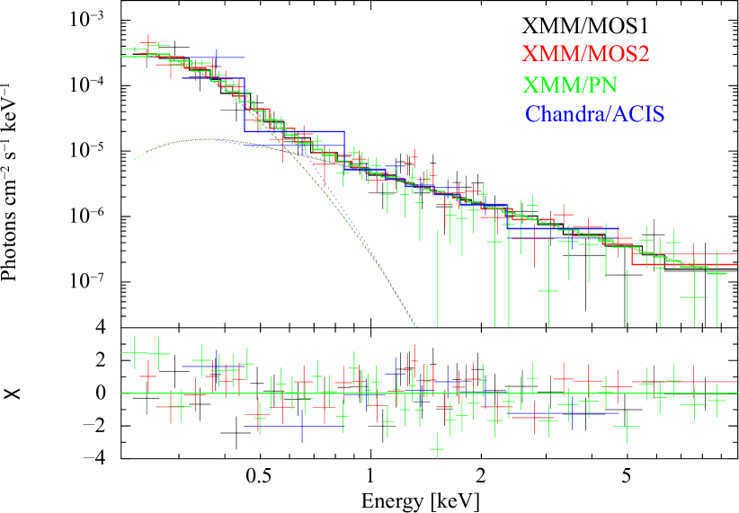
Figure 7: The J1957 unfolded spectrum and the model nsmdip1$+$PL with fixed angles at $\alpha$ = $66^{\circ}$ and $\zeta$ = $24^{\circ}$ (see the first line in Table 2). Dotted lines show the model components. Data from different instruments are indicated by different colours as indicated in the panel. Spectra were grouped to ensure at least 10 counts per energy bin for illustrative purposes.

4.2 The trail-like nebula

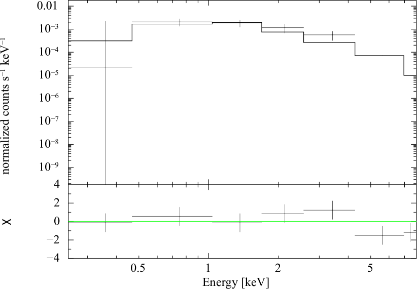
Figure 8: Chandra spectrum of the trail-like nebula, the best-fit PL model and residuals.

For the spectral analysis of the trail-like nebula, we used only the Chandra data set since in the XMM-Newton data it is somewhat blurred with several stars. We extracted spectrum of the trail using the 30 arcsec $\times$ 300 arcsec rectangle region shown in Fig. 5 together with the regions used for the background. It was binned to ensure at least 25 counts per energy bin and fitted in the 0.3–10 keV band. The total number of counts in the spectrum is 811 while only 105 of them come from the source. We tried the PL model and found that the column density is highly uncertain. Thus, we fixed it at $3\times 10^{20}$ cm^-2 which is compatible with all pulsar models (see Table 1). The resulting parameters $\Gamma=1.9\pm 0.5$, $K=7.3^{+1.9}_{-1.8}\times 10^{-6}$ ph cm^-2 s^-1 keV^-1, the unabsorbed flux in the 0.3–10 keV band $F_{X}=4.5^{+1.6}_{-1.1}\times 10^{-14}$ erg s^-1 cm^-2 and $\chi^{2}_{\nu}=1.17$ (dof = 29).

Such spectrum can have a synchrotron nature. The spectrum and the best-fit model are shown in Fig. 8. The spectrum can also be equally well described ($\chi^{2}_{\nu}=1.16$, dof = 29) by the thermal bremsstrahlung model with a temperature $3.6^{+12.1}_{-1.9}$ keV and the unabsorbed flux in the 0.3–10 keV band $F_{X}=3.7^{+1.8}_{-1.1}\times 10^{-14}$ erg s^-1 cm^-2.

5 Discussion

5.1 The pulsar spectral and timing properties

The time integrated X-ray spectrum of J1957 the in 0.15–10 keV range can be well described by the composite model consisting of the thermal and PL components while the single PL model suggested previously by Marelli et al. (2015) for a more narrow range of 0.3 – 10 keV is statistically unacceptable in the extended range. In the case of the BB + PL model, the obtained effective temperature $T^{\infty}\approx 54$ eV ($6.3\times 10^{5}$ K) is typical for the emission from the bulk of an NS surface but the radius of the emitting area is smaller than an expected NS radius of 10 – 15 km (see Table 1). The thermal emission could be produced by hot polar caps of the NS heated by relativistic particles from pulsar magnetosphere. For J1957, the ‘standard’ pulsar polar cap radius is about 0.3 km (Sturrock, 1971) which is compatible with the lower bound of the derived radius. However, the derived temperature is too low for the polar cap emission (cf. Potekhin et al., 2020), rejecting this possibility. Thus, the BB + PL model might describe some hotter part of the pulsar surface while the other part is cooler and not observed in X-rays as takes place, e.g., for the middle-aged PSR B1055$-$52 (Mignani, Pavlov & Kargaltsev, 2010). Note, however, that such interpretation implies that the obtained BB temperature cannot be used for a comparison with the predictions of the cooling theory; instead, the bolometric thermal luminosity should be used for such a comparison (as discussed, e.g., in Potekhin et al. 2020). Remarkably, the best-fitting thermal luminosities given by the BB+PL and nsmdip+PL models are compatible within uncertainties (see Table1).

The nsmdip$+$PL models also give acceptable fits. Although they are possibly less preferable according to the Bayesian criteria that disregard prior theoretical constraints on NS radii, they are more physically motivated. In particular, they are based on the magnetic atmosphere models, computed for realistic NS parameters, and they consistently take into account the distributions of temperature and magnetic field over the NS surface. Combining the results from all these models (Table 1), the estimated redshifted NS effective temperature $T^{\infty}\approx 20\pm 4$ eV ($0.23\pm 0.05$ MK). This makes the pulsar one of the coldest among all known NSs with estimated thermal luminosities, whose measured thermal emission from the surface is powered by cooling (see Section 5.3). We cannot constrain the pulsar viewing geometry (angles $\alpha$ and $\zeta$) from the time integrated spectra.

For the first time, we detected X-ray pulsations with the pulsar spin period. The pulsations are significant only in the soft band of 0.15–0.5 keV where the thermal emission component strongly dominates in the spectrum of the pulsar. The pulse profile is a sine-like with a single pulse per period and the pulsed fraction of $\approx 18\pm 6$ per cent, which is typical for thermal emission from a bulk of the surface of NSs (e.g. Pavlov & Zavlin, 2000a; Zavlin, 2009). This is independent confirmation of the results of the spectral analysis. The pulsations can be due to nonuniform temperature distribution over the surface of the NS due to magnetic anisotropy of the internal heat transfer to the star surface and the magnetic beaming of the radiation in its atmosphere. Both factors are accounted in our nsmdip models, while only the first one can provide pulsations for the BB model which may reminiscent of the emission from a solid state surface of the NS. In any case, using the BB model with a single temperature is a very rude simplification at the non-uniform temperature distribution over the star surface.

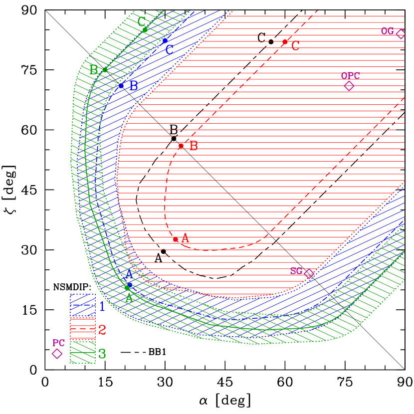
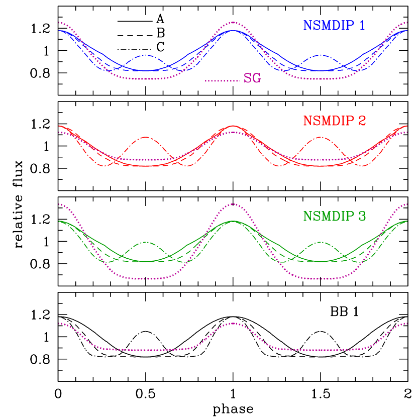
Figure 9: Left: Regions of magnetic obliquity $\alpha$ and rotation axis inclination $\zeta$ (hatched regions), compatible with the observed pulsed fraction $0.18\pm 0.06$ of emission in the soft X-ray energy band 0.15–0.5 keV, and the $\alpha$ and $\zeta$ combinations (curves) that provide the pulsed fraction 0.18, shown for the three nsmdip atmosphere models according to the legend. For comparison, a curve for a BB model (see text) is also plotted. The diagonal line separates the parts of the hatched regions in the lower triangle, which are compatible with the singe-pulsed light curves, as observed in Fig. 4. The violet diamonds show the tentative $\alpha$ and $\zeta$ values obtained by Pierbattista et al. (2015) using polar cap (PC), slot gap (SG), outer gap (OG) and one pole caustic (OPC) models of gamma-ray pulse formation. Right: Light curves in the redshifted energy band 0.15–0.5 keV, computed for models nsmdip 1, 2 and 3 at $\lg T^{\infty}\mbox{(K)}=5.4$ (the three upper panels) and the $\alpha$ and $\zeta$ angles shown by the respective points A, B and C in the left panel (solid, dashed, and dot-dashed lines). For comparison, the bottom panel shows the light curves computed for the best-fit BB model. The violet dotted line in each panel shows the light curve for $\alpha=66^{\circ}$ and $\zeta=24^{\circ}$ given by the fit with the SG model (Pierbattista et al., 2015).

The observed soft X-ray pulsations can be used to constrain the angles $\alpha$ and $\zeta$ that the rotation axis makes with the magnetic axis and the line of sight (magnetic obliquity and pulsar inclination), assuming that the flux in the photon energy band 0.15–0.5 keV is dominated by thermal emission. In the left panel of Fig. 9, the hatched regions correspond to the $\alpha$ and $\zeta$ values that provide the observed pulsed fractions of thermal radiation from 0.12 to 0.24 in the 0.15–0.5 keV energy band for the atmosphere models nsmdip 1–3, according to the legend. We see that for all the considered cases $\alpha+\zeta\ga 30^{\circ}$. Because of a higher redshift in model nsmdip 2, it shows a stronger gravitational light bending, which leads to a stronger smearing of the light curves, compared with the two other models. Therefore, higher $\alpha$ and $\zeta$ are needed to obtain the same pulsed fraction. In particular, the upper limit of 24 per cent is never reached (that is why the hatched area has a shape of a bell rather than a horseshoe in this case). The absence of an inter-pulse on the observed light curve in Fig. 4 suggests that $\alpha+\zeta\lesssim 90^{\circ}$. The curves in Fig. 9, left, show the combinations of $\alpha$ and $\zeta$ that provide the pulsed fraction 18 per cent. For comparison, we show an analogous line for the best-fitting BB model from Table 1 ($R^{\infty}=2.2$ km), assuming that thermal radiation comes from two uniformly heated circular regions around the poles on the surface of a star with the same $M=1.4\,\mbox{M${}_{\odot}$}$ and $R=12.6$ km as in models nsmdip 1 and 3. In contrast to the atmosphere radiation, which is has a peaked angular distribution, the BB radiation obeys the Lambert’s cosine law. For this reason, the same pulsed fraction is reached for higher $\alpha+\zeta$ values. For nsmdip 2, the above-mentioned smearing of the light curves due to the light bending effect is so strong that the pulsed fraction does not exceed 5 per cent, meaning that the BB model is inapplicable in this case. We also show the tentative $\alpha$ and $\zeta$ values obtained by Pierbattista et al. (2015), who fitted geometrical models to the observed $\gamma$-ray pulse profile, using different theoretical models of $\gamma$-ray pulse formation. We see that one of the models (the slot gap model) is compatible with nsmdip 1 and nsmdip 2. Examples of theoretical light curves, calculated as described in Appendix A, are shown in the right panel of Fig. 9. For each model we show three cases, marked by letters A, B and C, corresponding to the magnetic obliquity $\alpha$ and inclination $\zeta$ values shown in the left panel. Note, that case C does not agree with the observed profile since it predicts the presence of an inter-pulse and thus can be excluded.

The low number of counts does not allow us to perform the phase-resolved spectral analysis which could help to distinguish between different geometries and spectral models. Deeper X-ray observations are necessary to do that. Ultraviolet (UV) observations could also clarify the situation whether the thermal emission is best descried by the nsmdip or by the BB (solid state) spectral models as they predict different fluxes in this range.

Implementation of the extinction–distance relation in the fitting procedure allowed us to estimate the distance to J1957. We note, that due to the large relative uncertainties in this relation especially at low distances (see Appendix B), the constraints on $D$ are rather weak especially for the BB + PL model where $N_{\mathrm{H}}$ uncertainties are larger than for the atmosphere models. Thus, the BB + PL model gives the distance up to $\approx 1$ kpc while the nsmdip + PL models resulted in the range of 0.1–0.4 kpc. The former estimate is compatible with the ‘pseudo’-distance of 0.8 kpc (Marelli et al., 2015). Note,that the obtained distance range gives a reasonable $\gamma$-ray efficiency $\eta_{\gamma}=L_{\gamma}/\dot{E}$ of $\approx$0.006–0.6 where $L_{\gamma}=4\pi D^{2}G_{\rm 100}$ is the $\gamma$-ray luminosity and $G_{\rm 100}=2.6\times 10^{-11}$ erg s^-1 cm^-2 (Marelli et al., 2015) is the $\gamma$-ray flux above 100 MeV.

As for the PL spectral component, the derived photon index range of 1.5–1.9 is typical for pulsars (e.g. Kargaltsev & Pavlov, 2008). For all the models, the unabsorbed non-thermal flux in the 2–10 keV band is $F_{X}\approx 2\times 10^{-14}$ erg s^-1 cm^-2. This corresponds to X-ray luminosity $L_{X}$ of $\approx(0.24-3.83)\times 10^{29}$ erg s^-1 for the distance range of 100–400 pc provided by the atmosphere models and up to $2.4\times 10^{30}$ erg s^-1erg s^-1 with the upper bound on the distance of 1 kpc as provided by the BB model. The corresponding X-ray efficiency of $\eta_{X}=L_{X}/\dot{E}=10^{-5.34}-10^{-4.14}$ and up to $10^{-3.35}$, respectively. These values are compatible with empirical dependencies of pulsar X-ray nonthermal luminosity and efficiency vs. characteristic age (see e.g. Zharikov, Shibanov & Komarova, 2006; Zharikov & Mignani, 2013). Upper limits on the pulsed fraction in harder bands of $\approx 40-60$ per cent do not give any additional informative constraints on the properties of the non-thermal X-ray emission from the pulsar magnetosphere.

5.2 The nature of the trail-like nebula

As was noted in Section 2, there is a thin straight feature protruding north-west from the pulsar (in equatorial coordinates; Fig. 5) likely associated with it. Its spectrum can be well described by the PL model with parameters typical for X-ray synchrotron nebulae powered by pulsars, known as PWNe. Its length is $\approx 8$ arcmin which corresponds to $\approx 0.23-2.3$ pc for the obtained distance range of 0.1–1 kpc (see Table 1). This is compatible with lengths of other PWNe (e.g. Kargaltsev et al., 2017a).

We can assume that the J1957 moves in the south-east direction and thus the feature is a trail-like PWN as observed e.g. for PSR J1741$-$2054 (Auchettl et al., 2015). On the other hand, this can be a misaligned outflow which is not aligned with the pulsars’s proper motion (p.m.) direction (see e.g. Reynolds et al., 2017; Kargaltsev et al., 2017b, and references therein). If so, we do not see any hint of a ‘normal’ tail-like PWN protruding behind the pulsar in X-ray images. Torus or jet structures typical for PWNe of younger pulsars are also not detected. However, the situation can be similar to the Guitar nebula powered by PSR B2224+65: the guitar-shaped bow-shock nebula was detected in H$\alpha$ while no head-tail PWN was found within the shock in X-rays (Reynolds et al., 2017). Instead, X-ray observations revealed a jet-like feature inclined by $\approx 118$^∘ to the p.m. direction of B2224+65. For our pulsar, no H$\alpha$ emission was detected around it with the 3.6 m WIYN telescope at a 300 s exposure (Brownsberger & Romani, 2014). However, the exposure may be too short to detect a fainter bow-shock at a high galactic latitude of $\approx 11^{\circ}$ where the density of the interstellar matter is small and deeper observations are needed.

The tail interpretation suggests that J1957 should move towards the Galactic plane (Fig. 1) raising a question about its birth site somewhere in the Galactic halo. For the misaligned outflow, the direction of p.m. remains unclear. In the latter case, we can assume that J1957 was born in the Galactic disk since this possibility is more plausible than the birth in the halo. Due to the natal kick in the supernova explosion it could achieve high velocities and move away from the disk. In such a case, we can estimate the J1957 p.m. perpendicular to the Galactic plane. At the pulsar galactic latitude of $\approx 11^{\circ}$ the p.m. $\mu\approx 47\ t^{-1}_{\rm 840\ kyr}$ mas yr^-1, where $t_{\rm 840\ kyr}$ is the pulsar true age normalized to its characteristic age $t_{\mathrm{c}}$. This corresponds to the transverse velocity $v\approx 220\ t^{-1}_{\rm 840\ kyr}D_{\rm kpc}$ km s^-1 which is compatible with the pulsars velocity distribution (Hobbs et al., 2005) for the estimated distance range even if the true age is $\sim$5 times smaller.

The nebula spectrum can be also described by a thermal bremsstrahlung emission model with a temperature of $3.6^{+12.1}_{-1.9}$ keV. In this case the nebula emission comes from the shocked ISM and the pulsar p.m. must be aligned with the nebula axis. Such situation appears for the tail of PSR J0357+3205 (Marelli et al., 2013). However, due to low count statistics it is hard to distinguish between the PL and the thermal models in our case.

Measurement of the pulsar’s p.m. is necessary to understand the nature of the feature and deeper X-ray observations are needed to constrain its shape and spectral properties.

5.3 J1957 and the cooling theory

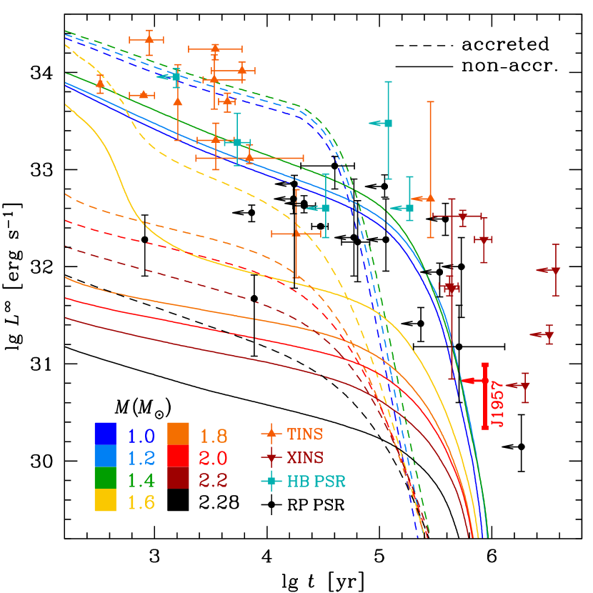
Figure 10: Cooling curves of NSs with different masses (coded with color), described by the EoS BSk24, for accreted and non-accreted heat blanketing envelopes, compared with observations. The data are plotted as indicated in the legend for NS classes following Potekhin et al. (2020): weakly magnetized thermally emitting isolated NSs (TINS), X-ray isolated NSs (XINS), high-B pulsars (HB PSRs) and rotation powered (‘ordinary’) pulsars (RP PSR). Vertical error bars show the estimated uncertainties on bolometric thermal luminosities, as seen by a distant observer. Horizontal error bars show the estimated age intervals, whenever available; otherwise horizontal arrows mark the characteristic ages (which are usually, although not always, larger than the true ages). The position of J1957 in this figure corresponds to the best-fitting model nsmdip 1, while the error bar embraces the models nsmdip 1–3 in Table 1.

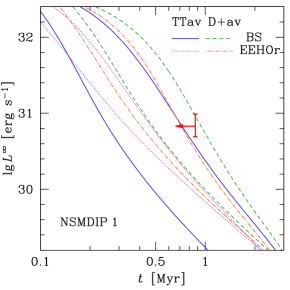
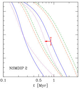
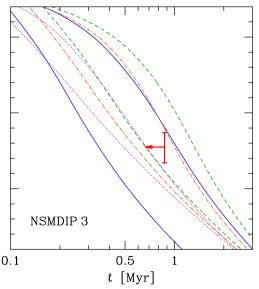
Figure 11: Late-time cooling of a strongly magnetized NS, consistent with the spectral fit models nsmdip 1, 2 and 3 (the left, middle and right panels, respectively). The EoS model BSk24 with $M=1.4\,\mbox{M${}_{\odot}$}$ is used for nsmdip 1 and 3, and BSk26 with $M=2\,\mbox{M${}_{\odot}$}$ is used for nsmdip 2. The polar magnetic field is $B_{\mathrm{p}}=3\times 10^{12}$ G (average $\langle B\rangle=2.2\times 10^{12}$ G) for nsmdip 1 and 2, while for nsmdip 3 we adopt $B_{\mathrm{p}}=1.1\times 10^{12}$ G ($\langle B\rangle=7.9\times 10^{11}$ G). Different line styles correspond to different models of baryon superfluidity in the stellar core, as shown in the legend: BS or EEHOr models for the proton pairing gap and TTav or D+av models for the neutron triplet pairing (see text). In each panel, the right/upper line of each type shows the cooling of a NS covered by a non-accreted magnetized heat blanket made of iron, while the left/lower line of each type corresponds to the fully accreted heat-blanketing envelope composed of layers of hydrogen, helium, carbon, and oxygen (Potekhin et al., 2003; Potekhin & Chabrier, 2018).

As noted above, J1957 can be one of the coldest cooling NSs with measured surface temperatures (e.g., Potekhin et al. 2020 and references therein). In Fig. 10 we compare the estimated thermal luminosities of different isolated NSs with theoretical cooling curves (i.e., redshifted luminosities as functions of ages). For J1957 we use the luminosity estimates reported in Table 1. The error bar unites the uncertainties for the models nsmdip 1–3. The model nsmdip 1 is adopted as the best estimate, because it provides the lowest BIC value among these three models. The observational estimates for the other cooling NSs are taken from Potekhin et al. (2020). For the NSs lacking timing-independent age estimates, including J1957, we plot $L^{\infty}$ against their characteristic ages $t_{\mathrm{c}}$. In these cases the leftward arrows indicate that $t_{\mathrm{c}}$ is likely to be larger than the true age, which is the common case, although there are exceptions where $t_{\mathrm{c}}$ is somewhat lower than the true age (see, e.g., examples, discussion and references in Potekhin et al. 2020). We see that J1957 has the lowest thermal luminosity among all cooling NSs with ages $<1$ Myr.

The theoretical cooling curves in Fig. 10 are calculated using the numerical code presented by Potekhin & Chabrier (2018). The BSk24 model (Pearson et al., 2018) is used for the composition and EoSp of the NS matter. The NSs are supposed to have either non-accreted (ground state) heat blanketing envelopes or accreted envelopes composed of helium, carbon, and oxygen up to the densities and temperatures where these chemical elements can survive (see, e.g., Potekhin et al., 2003; Potekhin & Chabrier, 2018). The accreted envelopes are more heat-transparent than the ground-state ones. For this reason, the stars with the accreted envelopes are brighter at the early stage of their evolution (at $t\lesssim 10^{4}$ yr), but they cool down faster and become colder at the late stage ($t\gtrsim 10^{5}$ yr). An envelope may consist of the accreted material only partially. In such cases the cooling rate is intermediate between the non-accreted and fully accreted extremes shown in the figure.

The critical temperatures for singlet neutron superfluidity in the inner crust and for proton and triplet neutron types of superfluidity in the core of a NS are evaluated, as functions of density, using the MSH, BS, and TTav parametrizations of Ho et al. (2015), which are based on theoretical models computed, respectively, by Margueron, Sagawa & Hagino (2008), Baldo & Schulze (2007), and Takatsuka & Tamagaki (2004). As can be seen from Fig. 10, thermal luminosity of J1957 is higher than the predictions of the cooling model for the age $t=t_{\mathrm{c}}$, so that theoretical cooling curves pass to the left of the error bar in this figure. However, as we mentioned above, it is likely that the true age $t$ is smaller than $t_{\mathrm{c}}$. If we treat $t_{\mathrm{c}}$ as an upper limit to the true age, than thermal luminosity of J1957 is compatible with the considered theoretical model. The smallest discrepancy between the best-fitting point and the theoretical cooling curves in Fig. 10 is observed for the model of an NS with $M\approx 1.4\,\mbox{M${}_{\odot}$}$, covered by the non-accreted heat-blanketing envelope. In this case, an agreement between the model and observations is reached, if we assume that $t\sim 0.5\mbox{~{}Myr}\sim 0.6t_{\mathrm{c}}$.

However, the cooling NS models shown in Fig. 10, being non-magnetic, are not fully consistent with the models of strongly magnetized atmosphere spectra (Appendix A). To produce cooling curves fully consistent with the spectral fitting, we employ a model of magnetized heat-blanketing envelope with mass $10^{-5}\,\mbox{M${}_{\odot}$}$. The bottom of such an envelope lies in a deep layer of the outer crust (at densities $\sim 10^{11}$ g cm^-3), which is nearly isothermal at the considered NS ages. The interior of a NS is treated as spherically symmetric, but temperature distribution in the envelope is essentially anisotropic. At the magnetic pole, the mechanical and thermal structure of the envelope is computed numerically, following Potekhin et al. (2003) and using updated microphysics input as per Potekhin & Chabrier (2018). Thermal conductivity treatment in the partially degenerate H and He layers of the accreted envelope has been updated following Blouin et al. (2020). The distribution of the effective temperature over the surface is then taken consistent with the dipole field, including the effects of General Relativity, as described in Appendix A. The interior of the star at densities $\gtrsim 10^{11}$ g cm^-3 is treated as spherically symmetric, with the microphysics (in particular, thermal conductivities, synchrotron neutrino emission rates, etc.) pertinent to the average magnetic field strength for each model. In the cases nsmdip 1 and 3 ($M=1.4\,\mbox{M${}_{\odot}$}$), we use the composition and EoS model BSk24, while for nsmdip 2 we use BSk26 (Pearson et al., 2018). The latter EoS is softer and provides the core composition preventing neutron star from the enhanced cooling at the assumed redshift $z_{\mathrm{g}}=0.44$, which corresponds to $M\approx 2\,\mbox{M${}_{\odot}$}$.

The results are shown in Fig. 11. To test the effects of baryon superfluidity we show, in addition to the models with the BS and TTav superfluidity of protons and neutrons (as in Fig. 10), also the cooling curves computed using alternative proton and neutron superfluidity models in the core. For an alternative proton superfluidity, we use the EEHOr parametrization by Ho et al. (2015) to the microscopic calculations of proton critical temperature by Elgarøy et al. (1996), which predicted substantially stronger proton superfluidity than BS. For an alternative superfluidity of neutrons, we use the ‘Av18 SRC+P’ model of Ding et al. (2016). which is marked ‘D+av’ in Fig. 11. In the latter case, the triplet neutron superfluidity is suppressed due to the effects of many-body correlations (although the maximum critical temperatures are similar in the TTav and D+av models, the latter model predicts a narrower range of densities where the neutrons are superfluid).

We see that the obtained estimates of thermal luminosity of J1957 can constrain the theoretical NS cooling models, constructed consistently with the fitting. Assuming that the true age of the pulsar does not exceed its characteristic age, we can conclude that the NS model nsmdip 1 is compatible with all employed models of superfluidity and envelope composition, but the NS models nsmdip 2 and 3 are hardly compatible with the suppressed neutron superfluidity (D+av), if the envelope is non-accreted. If we assume that the true age is close to $t_{\mathrm{c}}$, then for each spectral model we can select the best-fitting superfluidity and heat-blanketing envelope models in Fig. 11, for which the cooling curves are in a good agreement with the spectral fitting results. This reinforces the suggestion that the thermal-like part of the X-ray radiation of J1957 comes from the entire surface and is powered by passive cooling. Large uncertainties of the thermal luminosity provided by the BB model do not allow us to constrain cooling models.

6 Summary

Using the XMM-Newton and Chandra observations of the middle-aged $\gamma$-ray pulsar J1957, we detected, for the first time, the thermal spectral component and X-ray pulsations. We performed self-consistent modelling of thermal spectrum and cooling for models of NSs with strong dipole magnetic field. We applied it to the observations and estimated the J1957 thermal luminosity. It is consistent with the NS cooling theory and provides certain constraints on the NS model parameters. We found that J1957 is one of the coldest middle-aged NSs with measured effective temperatures: its redshifted thermal luminosity is $L^{\infty}\approx(0.2-1.0)\times 10^{30}$ erg s^-1. This indicates that J1957  has already passed from a relatively slow neutrino cooling stage to a significantly faster photon stage. The X-ray pulse-profile with a single pulse per period and with the pulse fraction of 18$\pm$6 per cent constraints the pulsar viewing geometry $30^{\circ}\lesssim\alpha+\zeta\lesssim 90^{\circ}$.

Using the interstellar extinction-distance relation, we estimated the distance to the pulsar to be of $\approx$0.1-1 kpc. Spectral fits with atmosphere models imply a most probable distance of 200 – 300  pc.

We also detected a weak $\sim$8 arcmin long trail-like feature connected with the pulsar. It most likely can be a PWN or a misaligned outflow powered by the pulsar.

Deeper X-ray observations are needed for more stringent constraints on the properties of the pulsar and the trail-like nebula. Phase-resolved analysis of such data could be helpful to understand the pulsar geometry. Measurement of the pulsar’s p.m. in X-rays is necessary to understand the nature of the nebula. Due to the low extinction and the likely proximity of J1957, it seems to be a good candidate for UV/optical observations. This could confirm the low temperature and lead to more accurate distance estimate.

Data Availability

The X-ray data are available through their respective data archives: https://www.cosmos.esa.int/web/xmm-newton/xsa for XMM-Newton data and https://cxc.harvard.edu/cda/ for Chandra data.

Appendix A Atmosphere models for neutron stars with dipole magnetic fields

Magnetized plane-parallel NS atmosphere models are computed using an advanced version of the code described in Suleimanov, Potekhin & Werner (2009). The code has been modified to account for different inclinations $\theta_{B}$ of the magnetic field with respect to the local surface normal. Hydrogen composition is considered, taking into account incomplete ionization at relatively low temperatures. The effects of the strong magnetic field and the atomic thermal motion across the field on the plasma opacities are treated following Potekhin & Chabrier (2003) with the improvements described in Potekhin, Chabrier & Ho (2014). Polarization vectors and opacities of normal electromagnetic modes are calculated as in Potekhin et al. (2004).

Physical models of emission from NSs should take into account magnetic field and temperature distributions over the surface. We assume a dipolar magnetic field, after accounting for the effect of General Relativity, according to Ginzburg & Ozernoy (1965) (see also Pavlov & Zavlin 2000b):

$$B=B_{\mathrm{p}}\,\sqrt{\cos^{2}\gamma+f^{2}\sin^{2}\gamma/4},\quad\cos\theta_{B}=(B_{\mathrm{p}}/B)\,\cos\gamma,$$ (1)

where $B$ is the field strength, $\theta_{B}$ is the field inclination to the surface normal at a magnetic colatitude $\gamma$,

$$f=\frac{2}{\sqrt{1-u}}\,\frac{u^{2}-2u-2(1-u)\,\ln(1-u)}{u^{2}+2u+2\,\ln(1-u)},$$ (2)

$u=r_{\mathrm{g}}/R$ is the compactness parameter, $r_{\mathrm{g}}=2GM/c^{2}$ is the gravitational radius, $G$ is the gravitational constant and $c$ is the speed of light. The distribution of local effective temperature $T_{\mathrm{s}}$ over the stellar surface is calculated using the results of Potekhin et al. (2003). In order to minimize model dependence, we assume the $T_{\mathrm{s}}$-distribution of an iron heat-blanketing envelope. This assumption does not change our results since, for any chemical composition of the envelope, the dependence of $T_{\mathrm{s}}$ on $\theta_{B}$ is similar to that given in Greenstein & Hartke (1983).

Model atmospheres for an inclined magnetic field require solving the transfer problem in two dimensions. The optical properties of the magnetized plasma depend on the angle $\eta$ between the photon wave vector $\bm{k}$ and the local magnetic field $\bm{B}$. On the other hand, under the plane-parallel approximation the radiation field naturally depends on the angles $(\theta_{k},\phi_{k})$, where $\theta_{k}$ is the angle between $\bm{k}$ and the surface normal and $\phi_{k}$ is the angle between the projections of $\bm{k}$ and $\bm{B}$ on the surface. To avoid interpolation of the opacities over such a two-dimensional grid, the code solves the transfer problem over an $(\eta,\psi)$ angular grid, where $\psi$ is the azimuth associated to the polar angle $\eta$, and then the transformation between the angular coordinates $(\eta,\psi)$ and $(\theta_{k},\phi_{k})$ is used (see Taverna et al. 2020 for more details):

$$\cos\eta = \sin\theta_{B}\sin\theta_{k}\cos\phi_{k}+\cos\theta_{B}\cos\phi_{k},$$ (3)

$$\cos\psi = \frac{\cos\theta_{k}-\cos\eta\cos\theta_{B}}{|\sin\eta\sin\theta_{B}|}.$$ (4)

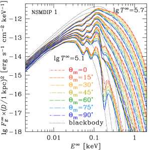
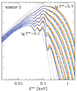
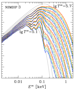
Figure 12: Unabsorbed redshifted spectral flux density as function of redshifted energy, calculated according to equation (8) for models 1, 2 and 3 listed in Table 3 (left, middle and right panels, respectively) for different inclinations $\Theta_{\mathrm{m}}$ of magnetic dipole axis (drawn with different line styles, according to the legend) and redshifted effective temperatures ($\lg T^{\infty}$ (K) = 5.1, 5.2, 5.3, 5.4, 5.5, 5.6 and 5.7, from bottom to top). For comparison, the BB spectra at the same temperatures are shown by dotted lines.

The photon wave-vector at infinity $\bm{k}^{\prime}$ differs from $\bm{k}$ at the surface due to gravitational redshift and light-bending (Pechenick, Ftaclas & Cohen, 1983; Pavlov & Zavlin, 2000b). The photon energy at infinity is smaller than the photon energy at the surface by factor $\sqrt{1-u}=1/(1+z_{\mathrm{g}})$, where $z_{\mathrm{g}}$ is gravitational redshift. The period of PSR J1957+5033 is sufficiently long so that we can assume that the stellar surface is spherical and neglect the effects of rotation (see, e.g., Poutanen & Beloborodov 2006 for description of these effects). Let us consider a surface element d$S=R^{2}\,\mathrm{d}\cos\vartheta\,\mathrm{d}\varphi$, where $\vartheta$ and $\varphi$ are the polar and azimuthal angles. For the relation between $\vartheta$ and $\theta_{k}$ we use approximation (Beloborodov, 2002)

$$1-\cos\vartheta=(1-\cos\theta_{k})/(1-u).$$ (5)

The flux observed from this surface element is proportional to the specific intensity $I_{E}^{\infty}$ and the solid angle $\mathrm{d}\Omega$ occupied by this element on the observer’s sky. This solid angle equals (Beloborodov, 2002)

$$\mathrm{d}\Omega=\frac{\mathrm{d}S\cos\theta_{k}}{D^{2}}\,\frac{1}{1-u}\,\frac{\mathrm{d}\cos\theta_{k}}{\mathrm{d}\cos\theta_{k}^{\prime}},$$ (6)

where $\theta_{k}^{\prime}$ is the angle between the local normal to the surface and the photon momentum at infinity. Without loss of generality we can choose the polar coordinate axis along the line of sight; then $\theta_{k}^{\prime}=\vartheta$. Since $I_{E}/E^{3}$ is invariant (Misner, Thorne & Wheeler 1973, Sect. 22.6), the observed specific intensity $I_{E}^{\infty}$ is related to the emitted intensity $I_{E}$ by a constant redshift factor $I_{E}^{\infty}=I_{E}/(1+z_{\mathrm{g}})^{3}$. Thus the flux is

$$\mathrm{d}F_{E}^{\infty}=I_{E}^{\infty}\mathrm{d}\Omega=\frac{R^{2}\cos\theta_{k}}{D^{2}}\frac{I_{E}}{(1+z_{\mathrm{g}})^{3}}\,\mathrm{d}\varphi\,\mathrm{d}\cos\vartheta.$$ (7)

The monochromatic spectral flux density is then computed by integrating the emission from different local patches over the stellar surface. Making use of equation (6), we obtain

$$F_{E}^{\infty}=\frac{R^{2}}{D^{2}(1+z_{\mathrm{g}})}\int_{0}^{2\pi}\!\!\mathrm{d}\varphi\int_{0}^{\pi/2}\!\!I_{E}(\theta_{k},\phi_{k})\cos\theta_{k}\sin\theta_{k}\mathrm{d}\theta_{k}.$$ (8)

For an axisymmetric magnetic field, the angle $\phi_{k}$ and the magnetic colatitude $\gamma$ are determined at every $\theta_{k}$ and $\varphi$ by the relations (cf. Ho et al. 2008)

$$\cos\gamma = \cos\varphi\sin\vartheta\sin\Theta_{\mathrm{m}}+\cos\vartheta\cos\Theta_{\mathrm{m}},$$ (9)

$$\cos\phi_{k} = \frac{\cos\gamma\cos\vartheta-\cos\Theta_{\mathrm{m}}}{|\sin\gamma\sin\vartheta|},$$ (10)

where $\Theta_{\mathrm{m}}$ is the angle between the magnetic axis and line of sight. The integration in equation (8) is restricted by those angles $\theta_{k}$ that correspond to real values of $\vartheta$.

Table 3: Parameter sets used in calculation of atmosphere models: cosines of magnetic colatitude $\gamma$ and magnetic field inclination $\theta_{B}$, logarithms of magnetic field strength $B$ and local effective temperatures $T_{\mathrm{s}}$.

$\lg T^{\infty}$ (K)			5.1	5.2	5.3	5.4	5.5	5.6	5.7
$\cos\gamma$	$\cos\theta_{B}$	$\lg B$ (G)	$\lg T_{\mathrm{s}}$ (K)
nsmdip 1: $M=1.4\,\mbox{M${}_{\odot}$}$, $R=12.6$ km ($z_{\mathrm{g}}=0.22$), $B_{\mathrm{p}}=3\times 10^{12}$ G
0.25	0.424	12.25	5.075	5.183	5.285	5.383	5.483	5.583	5.684
0.50	0.724	12.32	5.188	5.292	5.393	5.492	5.591	5.691	5.791
0.75	0.900	12.40	5.238	5.337	5.437	5.537	5.637	5.737	5.837
1	1	12.48	5.266	5.361	5.459	5.560	5.661	5.762	5.861
nsmdip 2: $M=2\,\mbox{M${}_{\odot}$}$, $R=11.4$ km ($z_{\mathrm{g}}=0.44$), $B_{\mathrm{p}}=3\times 10^{12}$ G
0.25	0.398	12.28	5.139	5.246	5.348	5.447	5.546	5.647	5.748
0.44	0.633	12.32	5.236	5.340	5.442	5.541	5.640	5.740	5.840
0.73	0.875	12.40	5.308	5.408	5.508	5.608	5.708	5.807	5.907
1	1	12.48	5.341	5.437	5.535	5.636	5.737	5.837	5.937
nsmdip 3: $M=1.4\,\mbox{M${}_{\odot}$}$, $R=12.6$ km ($z_{\mathrm{g}}=0.22$), $B_{\mathrm{p}}=1.1\times 10^{12}$ G
0.19	0.335	11.80	5.037	5.137	5.236	5.337	5.439	5.542	5.645
0.56	0.775	11.90	5.206	5.306	5.405	5.505	5.605	5.705	5.805
0.87	0.953	12.00	5.249	5.349	5.450	5.550	5.650	5.749	5.848
1	1	12.04	5.260	5.359	5.461	5.561	5.661	5.760	5.859

For each neutron star parameter set, the local plane-parallel atmosphere models are computed at the magnetic pole and at three magnetic latitudes between the pole and the equator, according to Table 3. The atmosphere model at the equator needs not to be calculated, because temperature at low latitudes is so low that it cannot noticeably affect the observed flux (in practice, we use the blackbody spectrum at the equator, but we have checked that with alternative models $F_{E}^{\infty}$ remains the same within 3 per cents). At each fixed magnetic colatitude $\gamma$, the opacities, polarizabilities, and EoS of the hydrogen plasma were computed on a fixed grid of plasma temperature and density, from which the values required during the radiative-transfer calculation were obtained by interpolation.

To calculate the integral (8), the specific intensity $I_{E}$ is evaluated at arbitrary $\gamma$, $E$, $\theta_{k}$ and $\phi_{k}$ from the computed values by interpolation. It should be noted that $B$-dependent absorption features would produce series of lines, if we kept $E$ fixed during this interpolation. In reality, such features are broadened due to the smooth variation of $B$ with $\gamma$. In order to reproduce this broadening and thus get rid of the non-physical series of lines, we first remap our calculated $I_{E}$ as a function of ratio $E/B$ and then interpolate it in $\theta_{k}$, $\phi_{k}$, and $B(\gamma)$ for every fixed $E/B$ (cf. Ho et al. 2008). The result of such integration is shown in Fig. 12.

The local effective temperature $T_{\mathrm{s}}$ and the global effective temperature $T_{\mathrm{eff}}$ are defined by the Stefan-Boltzmann law

$$\sigma_{\mathrm{SB}}T_{\mathrm{s}}^{4}=F_{r},\quad 4\pi R^{2}\sigma_{\mathrm{SB}}T_{\mathrm{eff}}^{4}=L_{r}$$ (11)

where

$$F_{r}=\int_{0}^{\infty}\mathrm{d}E\int_{0}^{2\pi}\mathrm{d}\phi_{k}\int_{0}^{\pi/2}I_{E}(\theta_{k},\phi_{k})\cos\theta_{k}\sin\theta_{k}\,\mathrm{d}\theta_{k}$$ (12)

is the local flux density, which depends on the magnetic colatitude $\gamma$, and

$$L_{r}=R^{2}\int_{0}^{2\pi}\mathrm{d}\varphi\int_{0}^{\pi}\,F_{r}(\gamma)\,\sin\vartheta\,\mathrm{d}\vartheta$$ (13)

is the local bolometric luminosity. The redshifted (‘apparent’) luminosity, effective temperature and radius as detected by a distant observer are (e.g., Thorne 1977)

$$L^{\infty}=L_{r}/(1+z_{\mathrm{g}})^{2}=4\pi\sigma_{\mathrm{SB}}(T^{\infty})^{4}(R^{\infty})^{2},$$ (14)

$$T^{\infty}=T_{\mathrm{eff}}/(1+z_{\mathrm{g}}),\quad R^{\infty}=R(1+z_{\mathrm{g}}).$$ (15)

For each model (nsmdip 1, 2 or 3), we fix radius $R$, redshift $z_{\mathrm{g}}$ and $B_{\mathrm{p}}$ to the values indicated in Table 3 and treat the effective temperature $T^{\infty}$, magnetic axis inclination $\Theta_{\mathrm{m}}$ and distance $D$ as continuous adjustable parameters to fit the observed spectral fluxes using calculated grids of $F_{E}^{\infty}$ .

In the axisymmetric model, the pulsar geometry is determined by the angles $\alpha$ and $\zeta$ that the spin axis makes with the magnetic axis and with the line of sight, respectively (e.g., Pavlov & Zavlin, 2000b). To produce phase-resolved spectra, it is sufficient to calculate

$$\cos\Theta_{\mathrm{m}}=\sin\zeta\sin\alpha\cos\phi+\cos\alpha\cos\zeta$$ (16)

for each rotation phase $\phi$. Some light curves computed by integration of such phase-resolved spectra are shown in Fig. 9.

Appendix B Interstellar absorption–distance relation

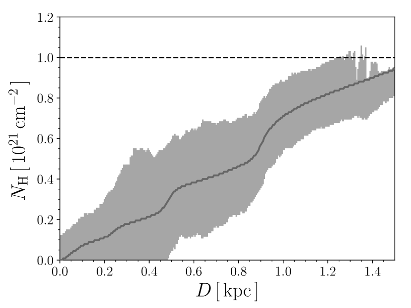
Figure 13: The relation between the interstellar absorption $N_{\mathrm{H}}$ and the distance $D$ (the dark gray line) with uncertainties shown in light gray in the direction towards J1957. The dashed black line shows the maximum $N_{\mathrm{H}}$ derived from the spectral analysis of two AGNi in the pulsar field (see text for details).

We estimated the distance to J1957 including the interstellar absorption–distance relation shown in Fig. 13 as a prior in the fitting procedure. The relation was derived in the following way. We used the 3D map of the local interstellar medium presented in https://stilism.obspm.fr/ (see Lallement et al. 2014; Capitanio et al. 2017; Lallement et al. 2018 for details) to obtain the relation between the interstellar extinction $E(B-V)$ and the distance $D$ in the pulsar direction. Then $E(B-V)$ was converted to the X-ray absorbing column density $N_{\mathrm{H}}$ utilising the relation by Foight et al. (2016). We used linear interpolation to derive the $N_{\mathrm{H}}$–$D$ dependence between the obtained points.

We also independently estimated the maximum absorption in the pulsar direction using two brightest extra-galactic X-ray sources in the J1957 field with coordinates R.A., Dec. = (19^h57^m16$.\!\!^{\mathrm{s}}$491, +50^∘40^′17$\aas@@fstack{\prime\prime}$280) and R.A., Dec. = (19^h56^m48$.\!\!^{\mathrm{s}}$205, +50^∘39^′32$\aas@@fstack{\prime\prime}$101). They have optical counterparts in the Pan-STARRS (Flewelling et al., 2016) and WISE (Cutri & et al., 2014; Schlafly et al., 2019) catalogues and are detected with the optical monitor (OM) on-board XMM-Newton. According to their spectral energy distributions, the sources are active galactic nuclei (AGNi). We extracted their X-ray spectra, grouped them to ensure at least 25 counts per energy bin and fitted with the absorbed model for AGN optxagn. The resulting column density $N_{\mathrm{H}}$ shown by the dashed black line in Fig. 13 is about 10²¹ cm^-2 which is in agreement with the value obtained from the $E(B-V)$–$D$ relation.

The spectral models which we used to describe the pulsar thermal emission includes the ratio of the emitting area radius and the distance as a parameter. Implementation of the $N_{\mathrm{H}}$–$D$ relation allowed us to separate it into two independent parameters.

References

- Abdo et al. (2013) Abdo A. A., et al., 2013, ApJS, 208, 17
- Arnaud et al. (2018) Arnaud K., Gordon C., Dorman B., 2018, Xspec: an X-Ray spectral fitting package. Users’ Guide for version 12.10.1. https://heasarc.gsfc.nasa.gov/xanadu/xspec/manual/XspecManual.html
- Auchettl et al. (2015) Auchettl K., et al., 2015, ApJ, 802, 68
- Baldo & Schulze (2007) Baldo M., Schulze H. J., 2007, Phys. Rev. C, 75, 025802
- Beloborodov (2002) Beloborodov A. M., 2002, ApJ, 566, L85
- Blouin et al. (2020) Blouin S., Shaffer N. R., Saumon D., Starrett C. E., 2020, ApJ, 899, 46
- Brazier (1994) Brazier K. T. S., 1994, MNRAS, 268, 709
- Brownsberger & Romani (2014) Brownsberger S., Romani R. W., 2014, ApJ, 784, 154
- Buccheri et al. (1983) Buccheri R., et al., 1983, A&A, 128, 245
- Capitanio et al. (2017) Capitanio L., Lallement R., Vergely J. L., Elyajouri M., Monreal-Ibero A., 2017, A&A, 606, A65
- Cash (1979) Cash W., 1979, ApJ, 228, 939
- Chang et al. (2012) Chang C., Pavlov G. G., Kargaltsev O., Shibanov Y. A., 2012, ApJ, 744, 81
- Cutri & et al. (2014) Cutri R. M., et al. 2014, VizieR Online Data Catalog, p. II/328
- Ding et al. (2016) Ding D., Rios A., Dussan H., Dickhoff W. H., Witte S. J., Carbone A., Polls A., 2016, Phys. Rev. C, 94, 025802
- Elgarøy et al. (1996) Elgarøy Ø., Engvik L., Hjorth-Jensen M., Osnes E., 1996, Phys. Rev. Lett., 77, 1428
- Flewelling et al. (2016) Flewelling H. A., et al., 2016, arXiv e-prints, p. arXiv:1612.05243
- Foight et al. (2016) Foight D. R., Güver T., Özel F., Slane P. O., 2016, ApJ, 826, 66
- Foreman-Mackey et al. (2013) Foreman-Mackey D., Hogg D. W., Lang D., Goodman J., 2013, PASP, 125, 306
- Ginzburg & Ozernoy (1965) Ginzburg V. L., Ozernoy L. M., 1965, Sov. Phys. JETP, 20, 689
- Goodman & Weare (2010) Goodman J., Weare J., 2010, Communications in Applied Mathematics and Computational Science, 5, 65
- Greenstein & Hartke (1983) Greenstein G., Hartke G. J., 1983, ApJ, 271, 283
- Ho et al. (2008) Ho W. C. G., Potekhin A. Y., Chabrier G., 2008, ApJS, 178, 102
- Ho et al. (2015) Ho W. C. G., Elshamouty K. G., Heinke C. O., Potekhin A. Y., 2015, Phys. Rev. C, 91, 015806
- Hobbs et al. (2005) Hobbs G., Lorimer D. R., Lyne A. G., Kramer M., 2005, MNRAS, 360, 974
- Kargaltsev & Pavlov (2008) Kargaltsev O., Pavlov G. G., 2008, in Bassa C., Wang Z., Cumming A., Kaspi V. M., eds, American Institute of Physics Conference Series Vol. 983, 40 Years of Pulsars: Millisecond Pulsars, Magnetars and More. pp 171–185 (arXiv:0801.2602), doi:10.1063/1.2900138
- Kargaltsev et al. (2017a) Kargaltsev O., Pavlov G. G., Klingler N., Rangelov B., 2017a, J. Plasma Phys., 83, 635830501
- Kargaltsev et al. (2017b) Kargaltsev O., Pavlov G. G., Klingler N., Rangelov B., 2017b, Journal of Plasma Physics, 83, 635830501
- Kerr et al. (2015) Kerr M., Ray P. S., Johnston S., Shannon R. M., Camilo F., 2015, ApJ, 814, 128
- Lallement et al. (2014) Lallement R., Vergely J. L., Valette B., Puspitarini L., Eyer L., Casagrande L., 2014, A&A, 561, A91
- Lallement et al. (2018) Lallement R., et al., 2018, A&A, 616, A132
- Manchester & Taylor (1977) Manchester R. N., Taylor J. H. J., 1977, Pulsars. W. H. Freeman & Co., San Francisco
- Marelli et al. (2013) Marelli M., et al., 2013, ApJ, 765, 36
- Marelli et al. (2015) Marelli M., Mignani R. P., De Luca A., Saz Parkinson P. M., Salvetti D., Den Hartog P. R., Wolff M. T., 2015, ApJ, 802, 78
- Margueron et al. (2008) Margueron J., Sagawa H., Hagino K., 2008, Phys. Rev. C, 77, 054309
- Mignani et al. (2010) Mignani R. P., Pavlov G. G., Kargaltsev O., 2010, ApJ, 720, 1635
- Misner et al. (1973) Misner C. W., Thorne K. S., Wheeler J. A., 1973, Gravitation. W. H. Freeman and Co., San Francisco
- Müller (2020) Müller B., 2020, Living Reviews in Computational Astrophysics, 6, 3
- Pavlov & Zavlin (2000a) Pavlov G. G., Zavlin V. E., 2000a, in Martens P. C. H., Tsuruta S., Weber M. A., eds, IAU Symposium Vol. 195, Highly Energetic Physical Processes and Mechanisms for Emission from Astrophysical Plasmas. p. 103
- Pavlov & Zavlin (2000b) Pavlov G. G., Zavlin V. E., 2000b, ApJ, 529, 1011
- Pearson et al. (2018) Pearson J. M., Chamel N., Potekhin A. Y., Fantina A. F., Ducoin C., Dutta A. K., Goriely S., 2018, MNRAS, 481, 2994
- Pechenick et al. (1983) Pechenick K. R., Ftaclas C., Cohen J. M., 1983, ApJ, 274, 846
- Pierbattista et al. (2015) Pierbattista M., Harding A. K., Grenier I. A., Johnson T. J., Caraveo P. A., Kerr M., Gonthier P. L., 2015, A&A, 575, A3
- Potekhin & Chabrier (2003) Potekhin A. Y., Chabrier G., 2003, ApJ, 585, 955
- Potekhin & Chabrier (2018) Potekhin A. Y., Chabrier G., 2018, Astronomy and Astrophysics, 609, A74
- Potekhin et al. (2003) Potekhin A. Y., Yakovlev D. G., Chabrier G., Gnedin O. Y., 2003, ApJ, 594, 404
- Potekhin et al. (2004) Potekhin A. Y., Lai D., Chabrier G., Ho W. C. G., 2004, ApJ, 612, 1034
- Potekhin et al. (2014) Potekhin A. Y., Chabrier G., Ho W. C. G., 2014, A&A, 572, A69
- Potekhin et al. (2020) Potekhin A. Y., Zyuzin D. A., Yakovlev D. G., Beznogov M. V., Shibanov Y. A., 2020, MNRAS, 496, 5052
- Poutanen & Beloborodov (2006) Poutanen J., Beloborodov A. M., 2006, MNRAS, 373, 836
- Reynolds et al. (2017) Reynolds S. P., Pavlov G. G., Kargaltsev O., Klingler N., Renaud M., Mereghetti S., 2017, Space Sci. Rev., 207, 175
- Saz Parkinson et al. (2010) Saz Parkinson P. M., et al., 2010, ApJ, 725, 571
- Schlafly et al. (2019) Schlafly E. F., Meisner A. M., Green G. M., 2019, ApJS, 240, 30
- Spitkovsky (2006) Spitkovsky A., 2006, ApJ, 648, L51
- Sturrock (1971) Sturrock P. A., 1971, ApJ, 164, 529
- Suleimanov et al. (2009) Suleimanov V., Potekhin A. Y., Werner K., 2009, A&A, 500, 891
- Takatsuka & Tamagaki (2004) Takatsuka T., Tamagaki R., 2004, Prog. Theor. Phys., 112, 37
- Taverna et al. (2020) Taverna R., Turolla R., Suleimanov V., Potekhin A. Y., Zane S., 2020, MNRAS, 492, 5057
- Thorne (1977) Thorne K. S., 1977, ApJ, 212, 825
- Willatt & Ehle (2016) Willatt R., Ehle M., 2016, Guide for use of the images script. https://www.cosmos.esa.int/documents/332006/641121/README.pdf
- Wilms et al. (2000) Wilms J., Allen A., McCray R., 2000, ApJ, 542, 914
- Yakovlev & Pethick (2004) Yakovlev D. G., Pethick C. J., 2004, ARA&A, 42, 169
- Yakovlev et al. (2005) Yakovlev D. G., Gnedin O. Y., Gusakov M. E., Kaminker A. D., Levenfish K. P., Potekhin A. Y., 2005, Nuclear Phys. A, 752, 590
- Zavlin (2009) Zavlin V. E., 2009, in Becker W., ed., Astrophysics and Space Sci. Library, Vol. 357, Neutron Stars and Pulsars. Springer, Berlin, p. 181
- Zharikov & Mignani (2013) Zharikov S., Mignani R. P., 2013, MNRAS, 435, 2227
- Zharikov et al. (2006) Zharikov S., Shibanov Y., Komarova V., 2006, Advances in Space Research, 37, 1979