Fermi Arc Reconstruction at the Interface of Twisted Weyl Semimetals

Abstract

Three-dimensional Weyl semimetals have pairs of topologically protected Weyl nodes, whose projections onto the surface Brillouin zone are the end points of zero energy surface states called Fermi arcs. At the endpoints of the Fermi arcs, surface states extend into and are hybridized with the bulk. Here, we consider a two-dimensional junction of two identical Weyl semimetals whose surfaces are twisted with respect to each other and tunnel-coupled. Confining ourselves to commensurate angles (such that a larger unit cell preserves a reduced translation symmetry at the interface) enables us to analyze arbitrary strengths of the tunnel-coupling. We study the evolution of the Fermi arcs at the interface, in detail, as a function of the twisting angle and the strength of the tunnel-coupling. We show unambiguously that in certain parameter regimes, all surface states decay exponentially into the bulk, and the Fermi arcs become Fermi loops without endpoints. We study the evolution of the ‘Fermi surfaces’ of these surface states as the tunnel-coupling strengths vary. We show that changes in the connectivity of the Fermi arcs/loops have interesting signatures in the optical conductivity in the presence of a magnetic field perpendicular to the surface.

I Introduction

Weyl semimetals Murakami2007 ; Wan2011 ; Yang2011 ; Burkov2011 ; Xu2011 ; Potter2014 ; Xu2015 ; Lv2015 ; Lu2015 ; Moll2016 are often described as three dimensional analogues of graphene graphene , with band-touchings or nodes at isolated points in the Brillouin zone. These nodes are chiral, and can be obtained by separating the Dirac nodes of a three dimensional semimetal by either time-reversal Murakami2007 or inversion symmetry Wan2011 ; Yang2011 ; Xu2011 ; Burkov2011 breaking. The low energy excitations about these nodes are Weyl fermions with anisotropic velocities that depend on the material parameters. Weyl semimetals (WSMs) exhibit several novel features such as negative longitudinal magneto-resistance Wan2011 ; Son2013 , anomalous Hall effect Xu2011 ; Yang2011 , chirality dependent Hall effect Yang2015 , planar Hall effect Nandy2017 , etc.

Several unconventional features have also been uncovered by studying transport across junctions of these Weyl semimetals with other topological and non-topological materials. For instance, junctions of Weyl semi-metals with superconductors have also led to new phenomena such as chirality dependent Andreev reflection Ueda2014 ; Bovenzi2017 and chirality dependent Josephson effects. Khanna2016 ; Khanna2017 Tunneling conductances across WSM-barrier-WSM junctions have also been studied with interesting experimentally testable consequences. Mukherjee2017 ; Mukherjee2019 ; Sinha2019

The band topology of the WSM is encoded in the monopole charge or the Chern number of the Berry curvature carried by the Weyl node. Hence surfaces in the bulk Brillouin zone (BZ) which enclose only one of the nodes carry Chern number. This leads to surface states called Fermi arc (FA) states in the surface BZ joining the projections of the Weyl nodes on to the surface BZ. Since the end-points of the FAs are the projections of the Weyl nodes, FAs on one surface connect to the FAs on the opposite surface through the bulk nodes. In the presence of a small magnetic field, this gives rise to intersurface cyclotron orbits Potter2014 which depend on the thickness of the sample. These exotic FA states are the hallmark of Weyl semimetals and it was their initial experimental identification Xu2015 using angle-resolved photoemission spectroscopy that led to the current explosion in theoretical interest Nonlocal2015 ; Deb2017 ; McCormick2018 in understanding their properties. More recently, Shubnikov-de Haas oscillations Moll2016 and the quantum Hall effect based on intersurface cyclotron orbits 3DQHE_WSM have been seen in $Cd_{3}As_{2}$.

Our aim in this work is to study the physics that emerges when two slabs of WSM are twisted with respect to each other and tunnel-coupled. From the analogy to graphene bilayers Novoselov2016 ; Duong2017 ; Mele2010 ; Mele2011 which show interesting effects, including the emergence of highly correlated states when the two layers have a small “magic angle” twist with respect to each other, Bistritzer2011 ; Sanjose2012 we might expect new physics, both in the bulk of the WSMs and in the interface FA states.

The WSM-WSM junction with no twist was initially studied in Refs. Dwivedi2018, ; Ishida2018, where FA reconstructions were found when the junction was between WSMs with different FA connectivities. Coupling of WSMs with small incommensurate twists has also been studied earlier by Murthy, Fertig, and Shimshoni Murthy2020 (henceforth MFS), in a perturbative regime of tunnel-coupling. MFS showed that, due to the effective Moire Brillouin zone that can be defined in terms of the mismatched lattice wave-vectors, reconstructions of the FAs take place. They also conjectured that at certain “arcless angles”, at sufficiently strong tunnel-coupling, the reconstructed surface states would consist of Fermi loops totally disconnected from the projections of the Weyl points on the surface BZ.

In this paper, we extend MFS’s work to arbitrary commensurate angles with a reduced lattice translation symmetry, and thus a larger superlattice unit cell at the interface. The presence of true lattice translation symmetry (absent in the work of MFS) allows us to analyze arbitrary strengths of the tunnel couplings between the two slabs. We perform a detailed study of the evolution of the FAs as a function of the coupling strength of the tunnel coupling for two sequences of commensurate twist angles parametrized by a positive integer $n$, $\theta_{n}=\tan^{-1}(1/n)$ and $\theta_{n}=\pi/2+\tan^{-1}(1/n)$. We unambiguously show that there exist parameter regimes where all the surface states are disconnected from the bulk, like the surface states of a topological insulator. We take a detailed look at the liftoff or detachment transition, where the Fermi arc detaches itself from the Weyl node projection and forms a surface state with a closed Fermi surface. We analyze the different ‘geometries’ into which the closed Fermi surfaces evolve. Finally, we uncover a duality between strong and weak interface tunnel couplings.

The plan of this paper is as follows. In Section II, we define our model Hamiltonian and the parameters that enter it, which include the commensurate twist angle and the interface hopping matrix. In Section III, we study the evolution of the interface FA states as a function of the twist parameter and the strength of the tunnel-coupling for two simple commensurate angles with the smallest superlattices at the interface, which display nearly all the phenomena of interest. In Section IV we present the simplest model of the liftoff or detachment transition, where the FA detaches itself from the Weyl point projection on the the surface BZ. We end in Section V with conclusions, caveats, a discussion of potential experimental signatures of the phenomena we uncover, and some promising future directions. Many important details of the calculations for larger interface superlattices, the symmetries of the model, the stability of our conclusions to longer range tunnel-couplings, etc are relegated to a series of appendices.

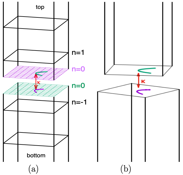
Figure 1: a) Two identical semi infinite WSM slabs are tunnel coupled. The coupling is parametrised by $\kappa$. The interface (at $z=0$) consists of two $n=0$ layers, one from the top slab and the other from the bottom slab. (b) The two slabs are twisted by $\theta$ clockwise and anticlockwise by the same angle and then coupled. For a commensurate twist angle $\theta$, there will be a superlattice(SL) at the interface (an example is shown in Fig. 2a).

II Twisted Weyl Semimetals and the Interface Hamiltonian

II.1 Time-reversal symmetry broken model of a WSM and its surface states

To set the notation for the interface states of two twisted WSMs, we briefly review the derivation of the surface states for a semi-infinite WSMMurthy2020 . We begin with a general two band lattice model of a time reversal symmetry broken WSM on a cubic lattice. The Hamiltonian in momentum space is

$$H_{0}= \sum_{\bf k}c^{\dagger}_{\bf k}\{2t^{\prime}\sin k_{z}\sigma_{z}+2\sin k_{y}\sigma_{y}$$

$$+2\sigma_{x}(2+\cos k_{0}-\cos k_{x}-\cos k_{y}-\cos k_{z})\}c_{\bf k}~{}.$$ (1)

The spectrum has Weyl nodes at $(\pm k_{0},0,0)$ with chirality $\pm 1$ respectively. Here $\sigma_{\mu}$, $\mu=(x,y,z)$ are the spin Pauli matrices and $c_{\bf k}=(c_{{\bf k}\uparrow},c_{{\bf k}\downarrow})^{T}$, are two component fermions. The hopping amplitude within the $x$-$y$ plane has been set to unity and $t^{\prime}$ represents the hopping amplitude along the $z$ direction. We choose our units so that the lattice constant $a$ can be set to unity throughout the paper. In this geometry, we expect Fermi arc states to be present on surfaces which are not normal to the $x$-axis, that is, those with surface Brillouin zones defined by $(k_{x},k_{y})$ or $(k_{x},k_{z})$.

To find the surface states, following Ref. Murthy2020, , we assume that the slab is semi-infinite in the $z$-direction, with lattice sites labeled by $n=0,1,2\dots$ and Fourier transform $H_{0}({\bf k})$ to real space (in the $z$ direction) to get

$$H_{0}(k_{x},k_{y}) =\sum_{n}\{2c^{\dagger}_{n}(f_{x}\sigma_{x}+f_{y}\sigma_{y})c_{n}-c^{\dagger}_{n}(\sigma_{x}+it^{\prime}\sigma_{z})$$

$$\hskip 17.07182pt\times c_{n+1}-c^{\dagger}_{n+1}(\sigma_{x}-it^{\prime}\sigma_{z})c_{n}\}$$ (2)

where $f_{x}=(2+\cos{k_{0}}-\cos{k_{x}}-\cos{k_{y}})$ and $f_{y}=\sin{k_{y}}$. We have suppressed the $k_{x},k_{y}$ dependence of all the fermion operators for notational simplicity. Following a rotation of the $\sigma$ matrices by $\pi/2$ around the $x$-axis, we get the transformed Hamiltonian to be

$$\tilde{H}_{0}(k_{x},k_{y}) =\sum_{n=0}^{\infty}\{2c^{\dagger}_{n}(f_{x}\sigma_{x}+f_{y}\sigma_{z})c_{n}-c^{\dagger}_{n}(\sigma_{x}-it^{\prime}\sigma_{y})$$

$$\hskip 17.07182pt\times c_{n+1}-c^{\dagger}_{n+1}(\sigma_{x}+it^{\prime}\sigma_{y})c_{n}\},$$ (3)

which turns out to be real and hence, more convenient for further analysis. As shown in detail in Ref. Murthy2020, , requiring the decaying solutions into the bulk to be normalizable, and assuming that $0<t^{\prime}=\sin\phi$ and $k_{0}<\phi$ gives the dispersion of the surface states as $E(k_{x},k_{y})=2f_{y}=2\sin{k_{y}}$ and the eigenstates are spin-polarized along the $\sigma_{z}$ direction.

II.2 Interface between two identical twisted WSMs

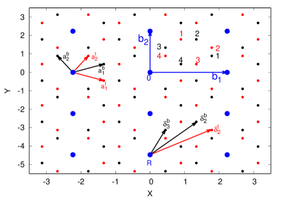
(a)

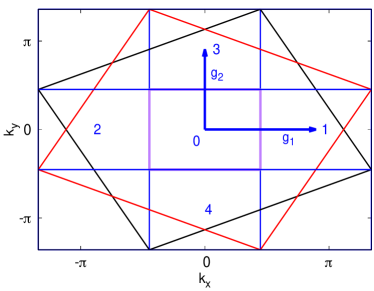
(b)

Figure 2: a) The interface layers for $n_{0}=2$. Here the top and bottom slabs are rotated by $\theta_{2}=\pm\tan^{-1}(1/2)$ so that the site $(2,1)$ of the $n=0$ layer of the top slab coincides with the $(2,-1)$ site of the $n=0$ layer of the bottom slab. The lattice sites of the top and bottom slab layers are in red and black colour respectively. The superlattice (SL) sites are in blue and ${\bf b}_{1}$, ${\bf b}_{2}$ are its primitive vectors.The SL unit cell contains $N_{sc}/2=2(n_{0}^{2}+1)/2=5$ lattice sites of each slab and they are labelled by $\alpha=\{0,1,2,3,4\}$. (b) Here, the Brillouin zones of the rotated slabs and of the SL lattice are shown. In addition to the first SL BZ (labelled $0$), the second BZs of the SL are also shown with labels $1,2,3$ and $4$ and ${\bf g}_{1},{\bf g}_{2}$ are the reciprocal lattice vectors of the SL. For this particular rotation, the SL BZ is $N_{sc}/2=5$ times smaller than the BZ of original lattice.

In this subsection, we will see how the Fermi arcs of two identical WSM slabs, twisted with respect to each other, get modified and reconstructed when we switch on a tunnel-coupling between them. We consider the interface of two identical WSMs as shown in Fig. 1. Both the WSMs are semi-infinite and the layers of the top slab are labeled by $n=0,1,2,..$ and the layers of the bottom slab are labeled by $n=0,-1,-2,..$. The interface consists of the zeroth layer of both the slabs, which are tunnel-coupled after twisting the top and bottom slabs around the z-axis by an angle $\pm\theta_{n_{0}}$ in the clockwise direction, analogous to the rotation of individual layers in bilayer graphene. Mele2010 The subscript $n_{0}$ indicates that we rotate the top slab clockwise and the bottom slab anticlockwise until the lattice site $(n_{0},1)$ of the top layer coincides with the lattice site $(n_{0},-1)$ of the bottom layer, where $n_{0}$ is a non negative integer. The twist angle in this case is clearly $\theta_{n_{0}}=\tan^{-1}(1/n_{0})$. This results in a periodic superlattice (SL) structure at the interface. We will consider only such commensurate twists in this paper.

The SL unit cell contains an equal number of lattice sites from the top layer and the bottom layer. For a given twist angle $\theta_{n_{0}}$, there are a total $N_{sc}=2\times(n_{0}^{2}+1)$ lattice sites per SL unit cell when $n_{0}$ is even (see Fig. 2a for an example when $n_{0}=2$). When $n_{0}$ is odd, then total number of lattice sites per SL unit cell are $N_{sc}=(n_{0}^{2}+1)$. For instance , when $n_{0}=0,1,2,3,4$ and $5$, the explicit number of total lattice sites per SL unit cell are $N_{sc}=2,2,10,10,34$ and $26$ respectively. The relative size (area) of the SL unit cell at the interface (with respect to the original 2D unit cell) is determined by $N_{sc}$ and it is actually $N_{sc}/2$ times larger.

In the presence of tunnel-coupling linking the top and bottom slabs, the full Hamiltonian consists of

$$H=H^{t}+H^{b}+\kappa H_{V}.$$ (4)

where the $t$ and $b$ refers to the top and bottom slabs and both of them are the same as $\tilde{H}_{0}(k_{x},k_{y})$ (Eq. II.1) except that the slabs are now rotated with respect to each other and $H_{V}$ is the coupling Hamiltonian (see Fig. 1). The overall strength of the coupling is parametrised by $\kappa$. The content of the spin-space matrix in $H_{V}$ will be described shortly. Since we started with a cubic lattice, the planar lattice is a square and after rotation, the primitive lattice vectors of the top layer are given by ${\bf a}^{t}_{1}=(\cos{\theta_{n_{0}}},-\sin{\theta_{n_{0}}}),{\bf a}^{t}_{2}=(\sin{\theta_{n_{0}}},\cos{\theta_{n_{0}}})$ and that of the bottom layer are ${\bf a}^{b}_{1}=(\cos{\theta_{n_{0}}},\sin{\theta_{n_{0}}}),{\bf a}^{b}_{2}=(-\sin{\theta_{n_{0}}},\cos{\theta_{n_{0}}})$ as shown in Fig. 2a (for $n_{0}=2$). The Hamiltonian is now explicitly given by

$$H^{\gamma}= \sum_{\bf k}\sum_{n}[2c^{\dagger}_{n}({\bf k}){\bf M}^{\gamma}c_{n}({\bf k})-c^{\dagger}_{n+1}({\bf k}){\bf T}c_{n}({\bf k})$$

$$\hskip 11.38092pt-c^{\dagger}_{n}({\bf k}){\bf T}^{\dagger}c_{n+1}({\bf k})]$$ (5)

where ${\bf k}$ here refers to the transverse momentum vector $(k_{x},k_{y})$ and $\gamma=(t,b)$ refer to the top and bottom layers, and the sum over $n$ goes from $n=0,1,2,\dots$ for the top layer and from $n=0,-1,-2,\dots$ for the bottom layer. The onsite and hopping matrices are given by

$${\bf M}^{\gamma} =(f_{1}^{\gamma}\sigma_{x}+f_{3}^{\gamma}\sigma_{z}),$$

$${\bf T} =(\sigma_{x}+it^{\prime}\sigma_{y});$$ (6)

with $f_{1}^{\gamma}({\bf k})=2+\cos k_{0}-\cos({\bf k.a}_{1}^{\gamma})-\cos({\bf k.a}_{2}^{\gamma})$ and $f_{3}^{\gamma}=\sin({\bf k.a}_{2}^{\gamma})$

As mentioned earlier, the interface consists of the zeroth layers of the WSM slabs, tunnel coupled by the hopping Hamiltonian $H_{V}$, given by

$$H_{V}=\sum_{{\bf r}_{t}}\sum_{{\bf r}_{b}}c^{\dagger}_{t0s}({\bf r}_{t})V_{ss^{\prime}}(|{\bf r_{t}-r_{b}}|)c_{b0s^{\prime}}({\bf r}_{b})+h.c,$$ (7)

where the lattice sites ${\bf r}_{t}$ and ${\bf r}_{b}$ live on the $n=0$ layer of the top and bottom slabs respectively. Note that we have now introduced the labels $t$ and $b$ to distinguish the fermions that live on the top and bottom layers. We have also introduced the spin indices $s$ and $s^{\prime}$ since the tunnel coupling is a matrix in spin space. We assume short-range hopping so that $V_{ss^{\prime}}$ is nonzero only for sites on the two surfaces with the same 2D coordinates.

$$V_{ss^{\prime}}(|{\bf r_{t}-r_{b}}|)=(V_{0})_{ss^{\prime}}\delta_{{\bf r}_{t},{\bf r}_{b}}.$$ (8)

These are the larger blue dots in Fig. 2a. In Appendix A, we show that the perturbative inclusion of longer-range hoppings does not qualitatively change the results that we obtain in our model.

Note that the most general tunneling matrix between two sites can be written as a matrix in spin-space,

$$V=\sum_{i=0}^{3}V_{i}\sigma_{i},$$ (9)

where $V_{i}$ are complex numbers, $\sigma_{0}$ is the identity matrix and $\sigma_{i}$ are the three Pauli matrices for $i=x,y,z$. This gives us a eight-parameter space of tunneling matrix elements, which is difficult to explore systematically.

Fortunately, there is a natural way to restrict the space of tunnel-couplings. When all tunneling matrix elements between the slabs are set to zero, our model (setting $\kappa=0$) enjoys a large number of symmetries, which include unitary, anti-unitary, particle-particle, and particle-hole type symmetries. For example, it is clear from Fig. 2a that, for $n_{0}=2$ the SL is symmetric about the positive diagonal with the replacement of sites $i=1,..4$ of the upper layer with the corresponding sites of the lower layer. It is also symmetric along the negative diagonal, with the replacement of the sites $1\leftrightarrow 3$ and $2\leftrightarrow 4$ between the upper and lower layers. These symmetries are detailed in Appendix B. In general, not all the symmetries of the uncoupled model can be satisfied by the tunneling term. We will assume that the tunneling conserves the symmetries of rotation by $\pi$ around both diagonals of the SL unit cell of the surface Brillouin zone for twist angles of the form $\theta_{n}=\pi/2+\tan^{-1}(1/n)$ . For $\theta_{n}=\tan^{-1}(1/n)$, on the other hand, we will assume symmetry of rotation by $\pi$ around the x and y axes. In both cases, this leads to a restriction that the tunneling matrix be real, and a combination of $\sigma_{x}$ and $\sigma_{y}$ only. It is thus of the form $V_{x}\sigma_{x}+iV_{y}\sigma_{y}$ where $V_{x},V_{y}$ are real. We have verified in Appendix C that perturbations violating these symmetries do not qualitatively change our conclusions.

To physically understand why $\sigma_{x}$ and/or $\sigma_{y}$ terms must be present in order to get a reconstructed Fermi arc at the interface, recall that the surface states of the top/bottom slabs are spin up/down polarized (see subsection II.1). So keeping solely $\sigma_{0}$ and/or $\sigma_{z}$ terms cannot lead to any coupling between the unreconstructed Fermi arcs of the top and bottom slabs.

III Interface states and their evolution

In this section, we will study the coupled FA states at the interface of the two WSMs. These are states that are localised on the interface and decay exponentially into the bulk. The individual FA eigenstates are Murthy2020 (details reviewed in Appendix D)

$$\ket{\Psi^{t}({\bf k})} =\sum_{n=0}^{\infty}\psi^{t}_{n}({\bf k})c^{\dagger}_{n}({\bf k})\ket{0}$$ (10)

$$\ket{\Psi^{b}({\bf k})} =\sum_{n=0}^{-\infty}\psi^{b}_{n}({\bf k})c^{\dagger}_{n}({\bf k})\ket{0}.$$ (11)

where $\psi^{t}_{n}({\bf k})\in\mathbb{C}^{2}$ ($n\geq 0$) and $\psi^{b}_{n}({\bf k})\in\mathbb{C}^{2}$ ($n\leq 0$) are wavefunctions, living on the $n$th layer, of the top and bottom slabs respectively. Since translational invariance is unbroken on the plane, the eigenstates can be labeled by the momenta ${\bf k}=(k_{x},k_{y})$.The two wave-functions of the zeroth layer - $\psi^{t}_{0}({\bf k})$, $\psi^{b}_{0}({\bf k})$ - are then matched at the interface in the presence of the coupling matrix $H_{V}$ given in Eq. 7. As shown in detail in Appendix D, the conditions for the existence of the interface states can be expressed as a matrix equation

$$M(E,\kappa,p_{x},p_{y})A=0,$$ (12)

where $M(E,\kappa,p_{x},p_{y})$ is a (not necessarily hermitian) square matrix of dimension $2N_{sc}\times 2N_{sc}$ and $A$ is a column matrix with $2N_{sc}$ rows (the factor of 2 is for the spin degrees of freedom). Here, we have used ${\bf p}=(p_{x},p_{y})$ to represent the momenta in the superlattice (SL) BZ. For interface localised states to exist, the determinant of the matrix must vanish. Therefore $\textrm{det}(M(E,\kappa,p_{x},p_{y}))=0$ gives a condition which $(p_{x},p_{y})$ must satisfy for a given $E$ and $\kappa$ to have the interface localised states.The set of all such $(p_{x},p_{y})$, for $E=0$ and fixed $\kappa$, yields the reconstructed Fermi arc state at the interface.

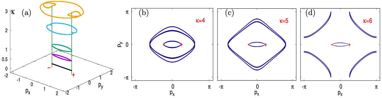
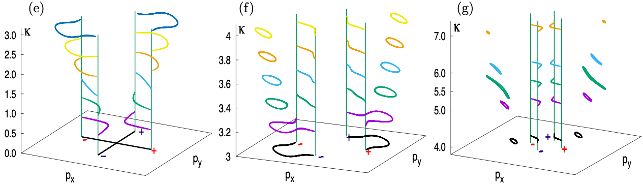
Figure 3: The panels show the evolution of the Fermi arcs (FAs) of the interface BZ as a function of the coupling strength. The panels in the top row are for $n_{0}=0$ and those in the bottom row are for $n_{0}=1$. (i) Panels (a),(b),(c) and (d) are for $n_{0}=0$ and a relative twist between the top and bottom slabs of $2\theta_{0}=\pi$. The positive (negative) chiral Weyl point projection (WPP) of the top slab and the negative (positive) chiral WPP of the bottom slab coincide at $(+(-)\pi/4,0)$ in the interface BZ. The parameters are $t^{\prime}=\sin{\pi/3}$, $k_{0}=\pi/4$ and $V_{x}=1,V_{y}=0$. When $\kappa=0$, the FAs of both the slabs are just straight lines along the $x$-axis between $(-\pi/4,\pi/4)$. When we switch on the coupling, the FAs evolve with increasing $\kappa$ as shown in panel (a). The vertical green lines represent the WPPs. For relatively higher values of $\kappa=4,5,6$, the reconstructed FAs are shown separately in panels (b), (c) and (d). (ii) Panels (e), (f), (g) and (h) are for $n_{0}=1$ and for different ranges of $\kappa$. The parameter values are the same as those for the top panels. Here, the relative twist between the slabs is $2\theta_{1}=\pi/2$. The unreconstructed FA for the bottom slab is along the y-axis and for the top slab, the unreconstructed FA is along the x-axis (shown as black lines in panel (e)). As a function of the coupling $\kappa$, the FAs go through a reconstruction which joins the two positive WPPs and the two negative WPPs of the two slabs together and for some values of $\kappa$ we see Fermi loops disconnected from the WPPs

To proceed further, we need to fix $n_{0}$ and explicitly find the FAs by solving $\textrm{det}(M(E,\kappa,p_{x},p_{y}))=0$. In the next subsection, we first consider the simplest cases, $n_{0}=0$ and $n_{0}=1$, with respective relative twist angles $2\theta_{0}=\pi$ and $2\theta_{1}=\pi/2$. In both cases, the two lattices are in registry and the full $xy$ translation symmetry of the original cubic lattice is present at the interface. In the following subsection, we will present results for the $n_{0}=2$ case in detail, with a larger interface unit cell, and therefore a reduced translation symmetry. The results for other twists (which are qualitatively similar) are presented in Appendix E.

III.1 Twists with ${\bf n_{0}=0}$ and ${\bf n_{0}=1}$

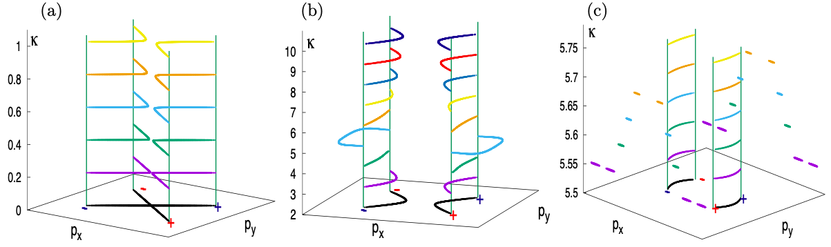
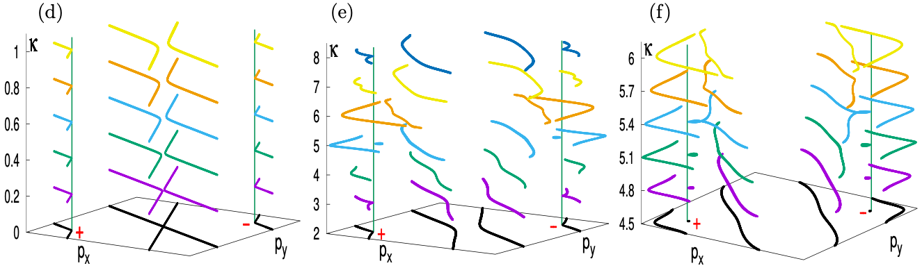
Figure 4: The panels show the evolution of the FAs at the interface BZ as a function of the coupling strength for $n_{0}=2$. (i) The panels in the top row show the evolution in the non-overlapping case where the Weyl point projections (WPPs) of the top (red $+$ve and $-$ve signs)and bottom slabs (black $+$ve and $-$ve signs) are distinct from each other. The vertical green lines represent the evolution of the WPPs. The parameters chosen are $t^{\prime}=\sin{\pi/3}$, and $V_{x}=1,V_{y}=0$. (a) Reconstructed FAs are shown for the coupling parameters in the range $\kappa=(0,1)$. For $\kappa=0$, the original FAs of the individual slabs are shown in black. As $\kappa$ increases, the reconstructed arcs join the $+$ve chirality WPPs together and the $-$ve chirality WPPs together (b) The range of the coupling is now from $\kappa=2$ to $\kappa=10$. (c) Shows the change of the sign of curvature of the FAs from positive to negative around $\kappa=5$ and formation of pairs of closed Fermi loop at the BZ boundary. These loops disappear pairwise after merging together around $\kappa=5.75$. (ii) The panels in the bottom row show the evolution when the WPPs of the top and bottom slabs overlap. The parameters chosen are $t^{\prime}=1.5$, $V_{x}=1$, $V_{y}=0.2$. (d) Evolution of the Fermi arcs for small $\kappa$. (e) The evolution shows the detachment of the FAs from the WPPs at around $\kappa\sim 3.5$. Also, the formation of a new small loop passing through the WPPS is seen around $\kappa\sim 5$. (f) A close-up view of the formation of the small closed loop passing through WPPs

To set the stage for studying arbitrary commensurate angles, we first study the case $n_{0}=0$. This case was studied earlier in Ref. Dwivedi2018, for the special case $t^{\prime}=1$ and the interface hopping being of the same form as the bulk hopping, except with a different strength. Here, we consider our more general model, and we consider the evolution of the FAs as a function of the coupling parameter. When the slabs are aligned, the Weyl point projections (WPPs) in the surface BZ of both the top and bottom slabs are at $(\pm k_{0},0)$ are on top of each other, with the positively charged chiral WPPs at $(k_{0},0)$ and the negatively charged chiral WPPs at $(-k_{0},0)$. In this case there need not be any states localized at the interface. However, when the two slabs are rotated by a relative angle of $2\theta_{0}=\pi$, the position of the positively charged chiral WPP of the top slab coincides, in the surface BZ, with the negatively charged chiral WPP of the bottom slab. Since the direction of the FA has changed between the slabs, the interface is well defined and there are necessarily interface localized states which get reconstructed as a function of the tunnel coupling. Note that the symmetry of the surface BZ under reflections about the $x$-axis and $y$-axis implies that the tunnel-couplings $V_{x}$ and $V_{y}$ in Eq. 9 can be chosen to be real and non-zero. For definiteness, we have chosen $V_{x}\neq 0$, although we have checked that taking a general linear combination of $V_{x}$ and $V_{y}$ does not change the result qualitatively. As mentioned above, the reconstructed FAs for $E=0$ and for a fixed coupling parameter $\kappa$ is given by the set of momenta $(p_{x},p_{y})$ for which the determinant of the $4\times 4$ matrix $M(E,\kappa,p_{x},p_{y})$ vanishes. The results are shown in the panels in the top row of Fig. 3 for a set of values of $\kappa$. At $\kappa=0$, the FA of the individual slabs are just straight lines on the $x$-axis between $(-k_{0},k_{0})$. With the increase in the coupling parameter $\kappa$, the FAs evolve as shown in Fig. 3(a). At $\kappa\sim 4$, in addition to the main FA connecting the WPPs, a pair of freestanding Fermi loops appear. For larger $\kappa$, the freestanding loops disappear and eventually, beyond the values shown in the graph, we get back the result for the FAs of the decoupled slabs. This is a particular instance of the duality in Fermi arc reconstruction under $\kappa\rightarrow 1/\kappa$ which is seen in all cases and which we shall discuss in detail later.

Next, let us consider the case when $n_{0}=1$. This was also earlier studied in Ref. Murthy2020, , but only for weak values of the coupling $\kappa$. When the slabs are rotated with respect to each other by an angle $2\theta_{1}=\pi/2$, the WPPs of one of the slabs in the surface BZ is $(0,\pm k_{0})$, whereas those of the other one are at $(\pm k_{0},0)$. As for $n_{0}=0$, the lattices are in registry and the reconstructed FAs are given by by a set of momenta $(p_{x},p_{y})$ for which the determinant of the $4\times 4$ matrix $M(E,\kappa,p_{x},p_{y})$ vanishes for a given $\kappa$ and for $E=0$. The results for the reconstructed FAs are shown in the bottom row of panels in Fig. 3. As expected, the FAs at zero coupling $\kappa$ are the FAs of the individual slabs. For the upper slab, it is a straight line on the $x$-axis and for the lower slab, it is a straight line on the $y$-axis. For nonzero $\kappa$, the reconstructed FAs connect the positively charged chiral WPPs and the negatively charged chiral WPPs of the slabs together as shown in Fig. 3(e). As $\kappa$ increases further, the FAs get deformed and a pair of freestanding closed loops form. For even larger $\kappa$, the freestanding loops disappear and eventually, as in the earlier case, the reconstructed FAs approaches the zero-coupling result.

III.2 Twist with ${\bf n_{0}=2}$

The simplest case where the surfaces of the top and bottom slabs are not in registry occurs for $n_{0}=2$, where the top and bottom slabs are twisted clockwise and counter-clockwise respectively by the angle $\theta_{2}=\tan^{-1}(1/2)$. This brings the lattice point $(2,1)$ of the bottom layer of the top slab lie on top of the $(2,-1)$ site of the top layer of the bottom slab, as shown in Fig. 2a, forming one of the sites of the superlattice (SL). As can be seen from the figure, the SL unit cell contains 5 lattice points from each of the layers ($N_{sc}=2\times(n_{0}^{2}+1)=10$ lattice sites altogether), and its unit cell is 5 times as large as the original unit cell. The primitive lattice vectors of the rotated slabs are now given by ${\bf a}_{t1}=(\cos{\theta_{2}},-\sin{\theta_{2}})$, ${\bf a}_{t2}=(\sin{\theta_{2}},\cos{\theta_{2}})$ for the top layer and ${\bf a}_{b1}=(\cos{\theta_{2}},\sin{\theta_{2}})$, ${\bf a}_{b2}=(-\sin{\theta_{2}},\cos{\theta_{2}})$ for the bottom layer. The superlattice primitive vectors are given by ${\bf b}_{1}=(\sqrt{5},0)$ and ${\bf b}_{2}=(0,\sqrt{5})$ and the SL unit cell contain total $N_{sc}=2(n_{0}^{2}+1)=10$ lattice sites as shown in Fig. 2a. The WPPs in the surface BZ of top slab are given by (i) $`+^{\prime}$ at $k_{0}(\cos{\theta_{2}},-\sin{\theta_{2}})$ and $`-^{\prime}$ at $k_{0}(-\cos{\theta_{2}},\sin{\theta_{2}})$ and that of bottom slab are given by (ii) $`+^{\prime}$ at $k_{0}(\cos{\theta_{2}},\sin{\theta_{2}})$ and $`-^{\prime}$ at $k_{0}(-\cos{\theta_{2}},-\sin{\theta_{2}})$. Note that our model does not specify $k_{0}$ - see Eq. 1 - it only says that the Weyl nodes are at $(\pm k_{0},0,0)$ - hence we are free to choose it to be any value consistent with the existence of FA states. Without loss of generality, we choose an arbitrary value of $k_{0}=\pi/4$.

The results for this case are shown in Fig. 4. As we turn on the coupling parameter $\kappa$, the reconstructed FAs connect the $+$ve chiral WPPs together (and the $-$ve chiral WPPs together). As $\kappa$ is increased, the curvature of the reconstructed FAs changes and flips sign near $\kappa\sim 5$ as shown in Fig. 4(b). This range of coupling $\kappa=(5.5,5.8)$ is explored further in Fig. 4(c), where a set of four small, closed, freestanding Fermi loops appear at the corners of the BZ when $\kappa\sim 5.55$. When $\kappa$ is further increased, they move towards each other, merge, and finally disappear at $\kappa\sim 5.75$. As for $n_{0}=0,1$, there is a duality in the FA reconstruction between small and large $\kappa$; at large $\kappa$ we get qualitatively the same FAs as small $\kappa$. In Fig. 4(b), one can see that the FAs at $\kappa=2,3$ are similar to the FAs at $\kappa=10,9$. Note that, in this case, we see that the reconstructed Fermi arcs are always attached to the WPPs.

Ref. Murthy2020, had conjectured that there might be arcless angles in twisted WSMs, where all interface states are disconnected from the WPPs. Can that occur in our model with commensurate twist angles as well? A precondition for this is to have WPPs of the same chirality from the top and bottom slabs overlap in the surface BZ. This can be achieved by combining a commensurate twist angle with a suitable choice of $k_{0}$. For example, at $n_{0}=2$, we rotate the top slab clockwise by an angle $\theta_{2}=\tan^{-1}(1/2)$ and the bottom slab by the angle $(\pi/2+\theta_{2})$ anti clockwise. The SL at the interface is identical to the earlier case, but the primitive lattice vectors are now given by ${\bf a}_{t1}=(\cos{\theta_{2}},-\sin{\theta_{2}})$, ${\bf a}_{t2}=(\sin{\theta_{2}},\cos{\theta_{2}})$ for the top slab and ${\bf a}_{b1}=(-\sin{\theta_{2}},\cos{\theta_{2}})$, ${\bf a}_{b2}=(-\cos{\theta_{2}},-\sin{\theta_{2}})$ for the bottom slab. Now we can choose $k_{0}=2\pi/3$ so that the positively charged chiral WPP of both the slabs coincide (and similarly the negatively charged chiral WPPs). The positively and negatively charged chiral WPPs are then at $k_{0}(\mp 1/\sqrt{5},\mp 1/\sqrt{5})$ in the surface BZ.

The reconstructed FAs in this case are shown in the panels in the bottom row of Fig. 4. Fig. 4(d) shows the situation for weak-coupling, where the FAs are attached to the WPPs. Fig. 4(e) reveals that FAs get detached from the WPPs for $\kappa\sim 3.5$ and move away from them as $\kappa$ increases. Subsequently a pair of small closed Fermi loops attached to the WPPs appear at $\kappa\sim 4.5$. Upon increasing $\kappa$ they disappear at $\kappa\sim 5.5$ (see Fig. 4(f)). So in the range of $\kappa$ between $3.5<\kappa<4.5$, and $5.5<\kappa<7.5$, the model has FAs which are wholly disconnected from the WPPs and there are no surface states attached to the WPPs. Beyond $\kappa=7.5$, the results are similar to the case when the couplings are small, because of the duality between large and small couplings.

We have also studied the twists with $n_{0}=4$ and $n_{0}=5$ for completeness. Since the results are qualitatively similar to the cases with smaller $n_{0}$, they are relegated to Appendix E.

IV Model for a lift-off transition

We have seen in the previous section that when the projections of the Weyl points of positive chirality coincide in the surface Brillouin zone (and likewise for the negative chirality Weyl points), the Fermi arc can detach from the WPP at an appropriate coupling strength $\kappa$. Because of the $\kappa\rightarrow 1/\kappa$ duality, the Fermi arc re-attaches again to the WPPs when $\kappa$ is increased and the reconstructed Fermi arc eventually approaches the unreconstructed Fermi arc in the limit $\kappa^{-1}\to 0$. In this section, our goal is to demonstrate these lift-off and re-attachment transitions in a simple model where there is no twist between the slabs. More specifically, we want to obtain the shape of the segment of the Fermi arc attached to the WPP at the transition, which, based on empirical evidence, we believe to be universal.

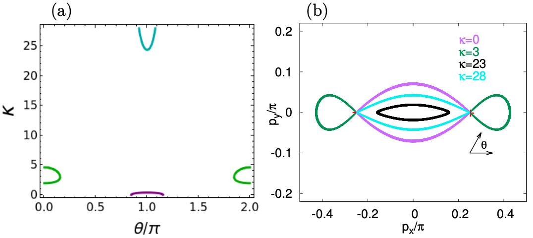
Figure 5: The lift-off transition (a) The curves denote the values of the coupling $\kappa$ as a function of $\theta$ for the existence of Fermi arcs in the vicinity of the Weyl point projection (WPP) at ${\bf k}=(\pi/4,0)$ and with $V=\sigma_{x}+it^{\prime}\sigma_{y}$. The parameters chosen are $\lambda=0.75$ and $t^{\prime}=0.8$. The solutions around $\theta=\pi$ correspond to the Fermi arcs which are in purple($\kappa=0$) and cyan($\kappa=28$) in figure (b), whereas the solutions around $\theta=0$(or $2\pi$) corresponds to the Fermi arcs in green. There are two $\kappa$ regions ( $0.37<\kappa<1.95$ and $4.62<\kappa<24.35$ ) where there are no Fermi arcs attached to the WPPs. As $\kappa$ is increased slowly from zero, the Fermi arc in purple colour in figure (b) evolves until it detaches from the WPPs at $\kappa_{c_{1}}\approx 0.37$. Then in the parameter regime, $0.37<\kappa<1.95$, there are no solutions until $\kappa_{c_{2}}\approx 1.95$. In the regime, $1.95<\kappa<4.62$, the Fermi arc in green evolves and detaches from the WPPs at the critical value $\kappa_{c_{3}}\approx 4.62$. Once again , there are no solutions when $4.62<\kappa<24.35$. Beyond $\kappa>24.35$ we get the dual solution, the Fermi arc in cyan in figure (b) which gradually approaches the zero coupling Fermi arc (in purple) as $\kappa\to\infty$.

We consider the Hamiltonian given in Eq. II.1 in the main text, but with a modified top/bottom-dependent $f_{y}$ term:

$$f_{y,\gamma}=\sin{k_{y}}+\lambda_{\gamma}(\cos{k_{x}}-\cos{k_{0}}).$$

For the top slab ($\gamma\equiv t$) we take $\lambda_{t}=\lambda$ and for the bottom slab ($\gamma\equiv b$), $\lambda_{b}=-\lambda$. There is no twist, but the slabs, though aligned, are not identical even in the bulk except at $\lambda=0$. We consider short-range hopping as before (Eq. 8) and the hopping matrix $V$ is taken to be $V=\sigma_{x}+it^{\prime}\sigma_{y}$.

As mentioned before, we need to compute the determinant of the matrix $M(E,\kappa,k_{x},k_{y})$ which is now a $4\times 4$ matrix, in the neighbourhood of the projection of the Weyl point. So we will parametrize the neighbourhood of the Weyl point projection ${\bf k}=(k_{0},0)$ in the surface BZ as

$$\vec{k}=k_{0}\hat{x}+\vec{q},\hskip 14.22636pt\vec{q}=q(\cos{\theta}\hat{x}+\sin{\theta}\hat{y}),$$ (13)

where $q=|\vec{q}|\ll 1$ and $\theta$ is the polar angle in the two-dimensional surface BZ around the Weyl point. The matrix $M(E,\kappa,k_{x},k_{y})$ can be explicitly written as

$$M=\begin{pmatrix}\frac{g_{1\uparrow}^{(t)}}{u_{1}^{(t)}}&\frac{g_{2\uparrow}^{(t)}}{u_{2}^{(t)}}&-\kappa g_{1\uparrow}^{(b)}&-\kappa g_{2\uparrow}^{(b)}\\ \frac{g_{1\downarrow}^{(t)}}{u_{1}^{(t)}}&\frac{g_{2\downarrow}^{(t)}}{u_{2}^{(t)}}&-\kappa g_{1\downarrow}^{(b)}&-\kappa g_{2\downarrow}^{(b)}\\ \kappa g_{1\uparrow}^{(t)}&\kappa g_{2\uparrow}^{(t)}&-\frac{g_{1\uparrow}^{(b)}}{u_{1}^{(b)}}&-\frac{g_{2\uparrow}^{(b)}}{u_{2}^{(b)}}\\ \kappa g_{1\downarrow}^{(t)}&\kappa g_{2\downarrow}^{(t)}&-\frac{g_{1\downarrow}^{(b)}}{u_{1}^{(b)}}&-\frac{g_{2\downarrow}^{(b)}}{u_{2}^{(b)}}\end{pmatrix}$$ (14)

where $u^{(t)}$ and $u^{(b)}$ are determined by Eqs. 40-41 and the various $g$’s are the components of the spin wavefunction of the top slab $\Phi^{t}=(g_{\uparrow}^{(t)},g_{\downarrow}^{(t)})^{T}$ and the bottom slab $\Phi^{b}=(g_{\uparrow}^{(b)},g_{\downarrow}^{(b)})^{T}$. The arguments of the matrix elements have been suppressed for notational simplicity. Our strategy is to Taylor expand each $u$ and $g$ to leading order in q. After some algebra, we get the following leading order expansions for the u’s :

$$u^{(t)}_{1} =1-\frac{q}{t^{\prime}}s_{t}(\theta),\hskip 14.22636ptu^{(b)}_{1}=1-\frac{q}{t^{\prime}}s_{b}(\theta),$$

$$u^{(t)}_{2} =u^{(b)}_{2}=\frac{1-t^{\prime}}{1+t^{\prime}}(1+\sin{k_{0}}~{}q\cos{\theta}),$$ (15)

where $s^{2}_{\gamma}(\theta)=(1+\lambda^{2})\sin^{2}{k_{0}}\cos^{2}{\theta}-\lambda_{\gamma}\sin{k_{0}}\sin{2\theta}+\sin^{2}{\theta}$.

To avoid singularities, we now divide the whole $\theta$ region into two sub regions - (i) $\pi/2<\theta<3\pi/2$ and (ii) $-\pi/2<\theta<\pi/2$ - and choose the spinors appropriately. The leading order expansions give the following solutions for the $g$’s -
In region (i) :

$$g^{(t)}_{1\downarrow} =\frac{\sin{\theta}-\lambda\sin{k_{0}}\cos{\theta}}{-\sin{k_{0}}\cos{\theta}+s_{t}(\theta)},\hskip 14.22636ptg^{(t)}_{2\downarrow}=\mathcal{O}(q^{2})$$

$$g^{(b)}_{1\uparrow} =-\frac{\sin{\theta}+\lambda\sin{k_{0}}\cos{\theta}}{-\sin{k_{0}}\cos{\theta}+s_{b}(\theta)},\hskip 8.5359ptg^{(b)}_{2\uparrow}=\mathcal{O}(q^{2})$$ (16)

where we have chosen $g^{(t)}_{1\uparrow}=g^{(t)}_{2\uparrow}=1$, $g^{(b)}_{1\downarrow}=g^{(b)}_{2\downarrow}=1$.
In region (ii):

$$g^{(t)}_{1\uparrow} =\frac{\sin{\theta}-\lambda\sin{k_{0}}\cos{\theta}}{\sin{k_{0}}\cos{\theta}+s_{t}(\theta)},\hskip 14.22636ptg^{(t)}_{2\downarrow}=\mathcal{O}(q^{2})$$

$$g^{(b)}_{1\downarrow} =-\frac{\sin{\theta}+\lambda\sin{k_{0}}\cos{\theta}}{\sin{k_{0}}\cos{\theta}+s_{b}(\theta)},\hskip 8.5359ptg^{(b)}_{2\uparrow}=\mathcal{O}(q^{2})$$ (17)

where we have chosen $g^{(t)}_{1\downarrow}=g^{(t)}_{2\uparrow}=1$, $g^{(b)}_{1\uparrow}=g^{(b)}_{2\downarrow}=1$.

We are interested in the existence of Fermi arcs in the vicinity of Weyl point projection. So for $q\ll 1$, we can approximate $u_{1}^{(t)}=u_{1}^{(b)}\approx 1$ and $u_{2}^{(t)}=u_{2}^{(b)}=u_{2}\approx\frac{1-t^{\prime}}{1+t^{\prime}}$ (see Eq. IV). This essentially implies that, very close to the Weyl point, the polar angle of ${\bf q}$, or the angle at which the FA attaches to the WPP, is the important parameter. Substituting these expressions in the matrix $M$, we get the following determinant vanishing conditions in the two regions -
For region (i) $\pi/2<\theta<3\pi/2$:

$$(\alpha_{t}\alpha_{b})\kappa^{4}+\frac{\kappa^{2}}{u_{2}^{2}}\left((1+u_{2}^{2})-2u_{2}(1+\alpha_{t}\alpha_{b})\right)+\frac{\alpha_{t}\alpha_{b}}{u_{2}^{2}}=0,$$ (18)

and for region (ii) $-\pi/2<\theta<\pi/2$:

$$\kappa^{4}+\frac{\kappa^{2}}{u_{2}^{2}}\left((1+u_{2}^{2})\alpha_{t}\alpha_{b}-2u_{2}(1+\alpha_{t}\alpha_{b})\right)+\frac{1}{u_{2}^{2}}=0,$$ (19)

where $\alpha_{t}=(\sin{\theta}-\lambda\sin{k_{0}}\cos{\theta})/(\sin{k_{0}}|\cos{\theta}|+s_{t}(\theta))$ and $\alpha_{b}=(\sin{\theta}+\lambda\sin{k_{0}}\cos{\theta})/(\sin{k_{0}}|\cos{\theta}|+s_{b}(\theta))$. The solutions to Eqs.18-19 for $\kappa$ as a function of $\theta$ give us the Fermi arcs attached to the WPP’s. The curves covered by these solutions are shown in Fig. 5(a) and in the remaining region, not covered by these lines, there are no Fermi arcs attached to the WPPs. Essentially, if there exist surface states in the remaining regions, those solutions are not coupled to the WPPs and would actually form closed Fermi surfaces. However, we do not study such solutions here since our aim here was to study the lift-off transition or the limits in the $(\kappa,\theta)$ space, where Fermi arcs attached to the WPPs are no longer present.

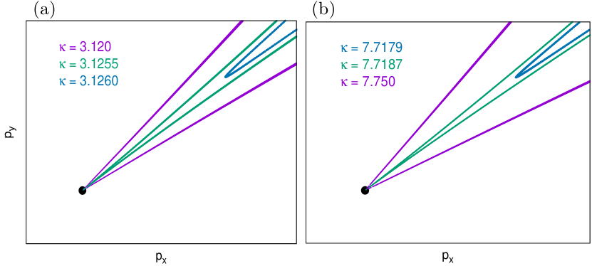
Figure 6: Singular shape of the Fermi arc near the (a) lift-off and (b) re-attachment transitions for $n_{0}=2$ (see also the reconstructed Fermi arc in Fig. 4(e)). The black dot in the figure represents the projection of negative chirality Weyl node.

We notice that at and near the lift-off (or re-attachment) transition, the shape of the Fermi arc is highly singular. The two legs that are attached to the WPP have the same slope at the transition. We believe this shape to be universal for all lift-off and re-attachment transitions, because in every instance of lift-off or re-attachment where we have “zoomed in” near the WPP at the transition, we find this to be the case. An example is shown in Fig. 6.

V Caveats, conclusions, discussion, and open questions

In this work we considered two identical semi-infinite slabs of WSM, twisted by a commensurate angle with respect to each other, and their free surfaces tunnel-coupled. The constraint that the angle be commensurate means that a reduced lattice translation symmetry, defined by a larger superlattice unit cell, is enjoyed by the Hamiltonian. This has the benefit of allowing us to extend our calculations to arbitrary values of the tunnel-coupling, which allowed us to extend the previous results of Murthy, Shimshoni, and Fertig Murthy2020 (which were for arbitrary small (incommensurate) angles, but perturbative values of the tunnel couplings.)

At this point it is important to mention several caveats concerning the assumptions we have made. Firstly, we focused most of our investigation on the case when the tunnel-couplings are ultra-short-range, being nonzero only for sites on the two surfaces having the same $xy$ coordinates. We did investigate longer-range hoppings as perturbations to this case (Appendix A), but did not undertake a study of the most general periodic hopping. Secondly, even with this simplification, the number of parameters in the hopping matrix is too large to allow systematic investigation. We therefore chose a particular subset of symmetries of the model system in the absence of tunnel-coupling, and imposed this symmetry on the tunnel-couplings as well. Once again, we have checked perturbatively that adding tunnel-coupling that break our self-imposed symmetries do not change our results qualitatively (Appendix C).

Three main results emerge from our work. Firstly, we confirmed an interesting conjecture from earlier work. MSF Murthy2020 considered (among other things) the case when the twist angle and the value of $k_{0}$ are tuned such that the WPPs of the $+$ Weyl nodes of the two slabs overlap (and likewise for the WPPs of the $-$ Weyl nodes). MSF conjectured that at strong enough tunnel-couplings the reconstructed Fermi arcs would detach themselves from the WPPs, leaving behind purely interface states, that is, states with all their spectral weight near the interface. We have confirmed that this appears to be a generic feature when the WPPs overlap. In addition, free-floating Fermi loops far from any WPP appear, expand, contract, and disappear as a function of the strength of the tunnel-coupling.

A noteworthy feature of such purely interface states (which they share with the surface states of topological insulators) is that some of them are two-dimensional states that cannot be obtained in a purely two-dimensional system of noninteracting electrons. For example, consider Fig. 10a, with $n_{0}=4$ and $\kappa=5.2$. The entire Fermi loop is one connected curve winding around the SL BZ (periodic boundary conditions apply at the boundaries of the SL BZ). However, it has no inside or outside. There is no notion of the number of states enclosed inside the Fermi surface.

Secondly, we identified a qualitative duality between weak and strong tunnel-couplings. This occurs for a very physical reason. Let us restrict ourselves to the case when the tunnel-couplings are “zero-range”, in the sense that the lattice sites of the two layers have to have identical $xy$ coordinates in order for the hopping to be nonzero. A very strong tunnel coupling $\kappa$ between the two vertically aligned sites, considered in isolation, will create a pair of hybridized states of energy of order $\pm\kappa$. Any tunneling between the slabs must go through these vertically aligned sites. Thus, the effective tunneling must be of order $t^{2}/|\kappa|$, where $t$ is the intra-slab tunneling strength. This shows that the two slabs become essentially isolated from each other as $|\kappa|\to\infty$. It may be possible to engineer large values of $|\kappa|$ in WSMs that cleave such that atoms on one WSM surface are likely to form covalent bonds with atoms on the other WSM surface.

Thirdly, we looked at the shape of the reconstructed Fermi arcs at the lift-off and re-attachment transitions. We found that they have a very singular shape, as demonstrated in Fig. 6. The singularity near the WPP also seems to be universal, in the sense that all lift-off and re-attachment transitions we have investigated in detail show the same shape near the WPP.

Let us examine potential experimental signatures of our theoretical results. First we consider the closed Fermi curves of purely two-dimensional interface states, as exemplified by Fig. 10a. Upon applying a weak (semiclassical) perpendicular orbital magnetic field, wave packets will experience a Lorentz force $-e{\bf v}({\bf k})\times{\bf B}$ where ${\bf v}({\bf k})={\bf\nabla}_{\bf k}\varepsilon({\bf k})$ is the group velocity of the Fermi loop states. Since the velocity is always perpendicular to the Fermi loop, the wave packets semiclassically travel along the closed Fermi curves. Under semiclassical quantization the states along the Fermi curve re-organize themselves into a set of equally spaced levels, with the the spacing directly proportional to $|{\bf B}|$. These levels can be investigated by the absorption of electromagnetic waves of the appropriate frequency.

How might one detect lift-off/reattachment transitions? A standard technique Potter2014 to look for Fermi arc states passing through the WPPs is to look at semiclassical orbits (once again under a weak perpendicular magnetic field) that traverse the Fermi arc on one surface, go through the bulk via the Weyl node to the other surface, traverse the Fermi arc there and complete the cycle.Such intersurface loops can enclose an area, and exhibit magneto-oscillations. Moll2016 The period of the cycle depends on the thickness of the slab. As usual, semiclassical quantization will reorganize the closed orbits into a set of equally spaced level, which can be investigated by an electromagnetic probe.

To be more specific on the experimental signature of the liftoff/re-attachment transitions, let us focus on the case when the WPPs overlap, and we are at weak-coupling, such that the Fermi arcs are attached to the WPPs. A wavepacket starting on the bottom surface of the lower slab will traverse the bulk of the lower slab through the Weyl node and reach the interface of the two slabs. At this point it will split; a part will traverse the Fermi arc at the interface, and another part will travel through the bulk of the upper slab, traverse the Fermi arc on the top surface of the upper slab, and return to the interface. Thus, there will be multiple scattering of the wavepacket, giving rise to a sequence of periods of return of the wavepacket to the bottom surface of the lower slab. Similarly, there will be a sequence of areas relevant to magneto-oscillations.

Now, if the tunnel-coupling is tuned such that the Fermi arcs detach from the WPPs, the interface is inaccessible to a wavepacket starting on the bottom surface of the lower slab. Thus, there is only one period of return for the wavepacket and only one area relevant to magneto-oscillations.

Thus, if an in-situ method (perhaps pressure) can be found to tune the strength of the tunnel-coupling through the lift-off/re-attachment transition, this abrupt change in behavior of the return period and/or magneto-oscillations will be a smoking-gun signature of such a transition.

The most important physics left out of our calculation is the effect of disorder. With regard to disorder, despite early work indicating the stability of the Weyl node against weak disorder, WSM+Disorder-early a consensus has emerged that large rare regions of strong disorder potential produce a nonzero density of states at the Weyl points, destroying the WSM even for arbitrarily weak disorder. WSM+Disorder-Global Similarly, the Fermi arcs get broadened by coupling to bulk disorder, and conduct dissipatively WSM+Disorder-dissipative-FA on short to intermediate length scales. They get localized at the longest length scales, but the chiral velocity persists at the surface. WSM+Disorder-FA Based on this picture, we can surmise that the Fermi loops traversing the superlattice BZ that we find in our work should be detectable as conducting states at all but the longest length scales. However, the states near the WPPs at the liftoff/re-attachment transitions will be particularly susceptible to disorder, and may be harder to detect via conduction.

There are many other interesting open questions, such as the possibility of interface quantum Hall effects and electron-electron interactions, which we hope to study in future work.

APPENDICES

The appendices provide details on: (a) The stability of FA reconstructions under longer ranged hoppings. (b) The symmetries of the $\kappa=0$ Hamiltonian in the superlattice Brillouin zone and the implications for tunnel-couplings. (c) The stability of FA reconstructions under perturbations of tunnelling matrix that break the above symmetries. (d) The details of the computation of the Fermi arcs at the interface. (e) Some illustrative results for larger values of $n_{0}$, or smaller twist angles.

Appendix A Stability of Fermi arc reconstructions under longer ranged hoppings

Figure 7: $n_{0}=2$: Long ranged couplings. The evolution of reconstructed Fermi arcs as a function of the coupling range parameter $\xi$ is shown for different fixed coupling strengths $\kappa$. The parameters are $k_{0}=2\pi/3,t^{\prime}=1.5$, $V_{x}=1,V_{y}=0$. (a) and (b) show the evolution of the reconstructed Fermi arcs with $\xi$ for $\kappa=0.2$. When $\xi$ is small we recover our previous short-range coupling results(see Fig. 4d) and it is clear that the results are stable with the increase in the range of the couplings. (c) Here, the coupling strength is fixed at $\kappa=4$ to examine the stability of the Fermi arc detachment from WPPs. $\xi$ is kept small because the effective strength of the coupling gets renormalized to larger value with increasing $\xi$. Note that in (c), the reconstructed Fermi arcs around ‘+’ WPP and ‘-’ WPP are not symmetric for larger values of $\xi$. Indeed, we do not expect the symmetry between the Weyl node projections to exist for a general $\xi$.

So far we have discussed results where the hoppings between the top and bottom layers are taken to be ultra-short range, such that only sites of the top and bottom slabs with the same 2D coordinates are tunnel-coupled. It is natural to ask what happens to the Fermi arc states at the interface if the range of the hoppings were increased to also include the next nearest sites and the next-next nearest sites and so on. We attempt to answer this question here by considering the hopping $V_{ss^{\prime}}({|{\bf r}_{t}-{\bf r}_{b}|})$ as a Gaussian,

$$V_{ss^{\prime}}(|{\bf r}_{t}-{\bf r}_{b}|)=\kappa(V_{0})_{ss^{\prime}}e^{-\frac{r^{2}}{\xi^{2}}}.$$ (20)

Here $(V_{0})_{ss^{\prime}}$ is a constant matrix, $\kappa$ denotes the strength of the interaction and $\xi$ is a length scale parameter that determines the range of hopping. Small(large) $\xi$ means that the hopping is short(long) ranged. For $\xi<<1$, we should recover our previous results, which was for ultra-short range hopping. Without loss of generality, we study the case $n_{0}=2$. In particular, we consider the case with overlapping Weyl point projections(WPPs).

The results are shown in Fig. 7. We have studied how the reconstructed Fermi arcs get modified as a function of the hopping range parameter $\xi$. We have considered two different coupling strengths $\kappa=0.2$ and $\kappa=4$. Since the effective coupling strength parameter $\kappa e^{-{r^{2}}/{\xi^{2}}}$ gets renormalized to larger value with increasing hopping range $\xi$, we restrict the hopping range parameter to smaller values for the latter case $\kappa=4$. We recover our previous results of short range hopping for very small $\xi<<1$. We find that the short-range hopping result is stable against longer ranged hoppings unless $\xi$ is too large.

Appendix B Symmetries of the $\kappa=0$ Hamiltonian in the superlattice Brillouin zone

In the main text, we have mentioned that the symmetries of the Hamiltonian of the slabs ($H^{t}+H^{b}$) can be kept intact if we restrict the tunnelling matrix to be of the following form $V=V_{x}\sigma_{x}+iV_{y}\sigma_{y}$, where $V_{i}$ ($i=x,y$) is a real number. We will show this result here explicitly for a particular value of the twist angle $\theta_{n_{0}=2}$; however, the result is general and is valid for all $n_{0}$ .

We will consider the case $n_{0}=2$ with overlapping Weyl point projections (WPPs) i.e. for commensurate twist angle of the form $\theta_{n_{0}}=\pi/2+\tan^{-1}(1/n_{0})$. The resulting superlattice (SL) is identical to what is shown in Fig. 2a (but now with differently oriented lattice vectors ${\bf a}^{\gamma}_{i}$, where $\gamma=t,b$ and $i=1,2$). To analyse the symmetries, it is convenient to take the Hamiltonian (in Eq. II.2) in the position space in all directions -

$$H^{\gamma}=\sum_{{\bf n}} \hskip 8.5359pt2(2+\cos{k_{0}})c^{\dagger}_{s}({\bf n})(\sigma_{x})_{ss^{\prime}}c_{s^{\prime}}({\bf n})$$

$$-\left(c^{\dagger}_{s}({\bf n+a}_{1}^{\gamma})(\sigma_{x})_{ss^{\prime}}c_{s^{\prime}}({\bf n})+h.c.\right)$$ (21)

$$-\left(c^{\dagger}_{s}({\bf n+a}_{2}^{\gamma})(\sigma_{x}-i\sigma_{z})_{ss^{\prime}}c_{s^{\prime}}({\bf n})+h.c.\right)$$

$$-\left(c^{\dagger}_{s}({\bf n+a}_{3}^{\gamma})(\sigma_{x}+it\sigma_{y})_{ss^{\prime}}c_{s^{\prime}}({\bf n})+h.c.\right).$$

Here ${\bf n}=n_{1}{\bf a}_{1}^{\gamma}+n_{2}{\bf a}_{2}^{\gamma}+n_{3}{\bf a}_{3}^{\gamma}$ with $n_{i}$ (i=1, 2, 3) are integers, and ${\bf a}_{i}^{\gamma}$ are the primitive lattice vectors. For the top slab $\gamma\equiv t$, $n_{3}$ runs over the range $(0,\infty)$ and for the bottom slab $\gamma\equiv b$, $n_{3}$ runs over the range $(0,-\infty)$.

The periodicity at the interface is that of the SL, so we need to express the operators in terms of the SL site labels. So we rewrite the operators as follows: $c_{s}({\bf n})=c_{s}({\bf R}+{\boldsymbol{\delta}}_{\alpha},n_{3})\equiv d_{\alpha s}({\bf m},n_{3})$ for the top slab ($n_{3}\geq 0$) and $c_{s}({\bf n})=c_{s}({\bf R}+{\boldsymbol{\delta}}_{\alpha},n_{3})\equiv f_{\alpha s}({\bf m},n_{3})$ for the bottom slab ($n_{3}\leq 0$). Here $\alpha$ is the sublattice index and ${\bf R}=m_{1}{\bf b}_{1}+m_{2}{\bf b}_{2}$ is the position vector of SL sites (see Fig. 2a). By inspection, it is clear that there are geometric symmetries of the model that involve rotation of the lattice by $\pi$ around both diagonals ( $i.e.$, the sites in black and red in Fig. 2a get interchanged). We will now see how these symmetries are implemented in terms of $d_{\alpha s}({\bf m},n_{3})$ and $f_{\alpha s}({\bf m},n_{3})$.

First, let us consider the symmetry transformation associated with the $\pi$ rotation about $m_{1}=m_{2}$ diagonal.

(i) $$U_{1}d_{\alpha s}(m_{1},m_{2},n_{3})U^{\dagger}_{1}=(\sigma_{x})_{ss^{\prime}}f_{\alpha s^{\prime}}(m_{2},m_{1},n_{3})$$

$$U_{1}iU^{\dagger}_{1}=i,\hskip 8.5359ptU_{1}VU_{1}^{\dagger}=\sigma_{x}V^{\dagger}\sigma_{x}$$ (22)

where the symmetry is unitarily realised and of the particle-particle type, and

(ii) $$Q_{1}d_{\alpha s}(m_{1},m_{2},n_{3})Q^{\dagger}_{1}=(i\sigma_{y})_{ss^{\prime}}f^{\dagger}_{\alpha s^{\prime}}(m_{2},m_{1},n_{3})$$

$$Q_{1}iQ_{1}^{\dagger}=i,\hskip 8.5359ptQ_{1}VQ_{1}^{\dagger}=-\sigma_{y}V^{T}\sigma_{y}$$ (23)

where again, the symmetry is unitarily realised, but is of the Boguliobov or particle-hole type.

Note that the spatial arguments of the fermion operators are not the same on both the sides of the equation - in fact because the spatial transformation involves a rotation of the lattice by $\pi$ about the diagonal, $m_{1}\leftrightarrow m_{2}$. After lengthy algebraic manipulations, it can be shown that both the symmetry transformations interchange $H^{t}$ and $H^{b}$ - $i.e.$, $U_{1}H^{t}U_{1}^{\dagger}=H^{b}$ and $Q_{1}H^{t}Q_{1}^{\dagger}=H^{b}$, and vice-versa. So if we require both the transformations to be symmetries of the Hamiltonian, then we need the tunnelling matrix to be of the form $V=V_{x}\sigma_{x}+iV_{y}\sigma_{y}$ where $V_{i}(i=x,y)$ are real numbers (assuming also that $V$ has to be real). This is clear since the transformation (i) will be a symmetry of the total Hamiltonian $H=H^{t}+H^{b}+H_{V}$, only if the tunnelling matrix $V$ satisfies the condition

$$U_{1}VU_{1}^{\dagger}=\sigma_{x}V^{\dagger}\sigma_{x}=V,$$ (24)

and the transformation (ii) will be a symmetry of H only if $V$ obeys the condition

$$Q_{1}VQ_{1}^{\dagger}=-\sigma_{y}V^{T}\sigma_{y}=V.$$ (25)

There are also symmetry transformations associated with $\pi$ rotation around the other diagonal $m_{2}=-m_{1}$ of the SL. In this case we have the following anti-unitary symmetry transformations:

(iii) $$U_{2}d_{\alpha s}(m_{1},m_{2},n_{3})U_{2}^{\dagger}$$

$$=(S)_{\alpha\alpha^{\prime}}(\sigma_{x})_{ss^{\prime}}f_{\alpha^{\prime}s^{\prime}}(-m_{2},-m_{1},n_{3})$$

$$U_{2}iU_{2}^{\dagger}=-i,\hskip 8.5359ptU_{2}VU_{2}^{\dagger}=\sigma_{x}V^{T}\sigma_{x}$$ (26)

of the particle-particle type and

(iv) $$Q_{2}d_{\alpha s}(m_{1},m_{2},n_{3})Q_{2}^{\dagger}$$

$$=(S)_{\alpha\alpha^{\prime}}(i\sigma_{y})_{ss^{\prime}}f^{\dagger}_{\alpha^{\prime}s^{\prime}}(-m_{2},-m_{1},n_{3})$$

$$Q_{2}iQ_{2}^{\dagger}=-i,\hskip 8.5359ptQ_{2}VQ_{2}^{\dagger}=-\sigma_{y}V^{\dagger}\sigma_{y}.$$ (27)

of the Boguliobov type. Note also that here the geometric symmetry interchanges $m_{1}\leftrightarrow-m_{2}$. The matrix in the sublattice index $S_{\alpha\alpha^{\prime}}$ has the following non zero elements $S_{00}=1,S_{13}=S_{31}=1,S_{24}=S_{42}=1$. Both the above transformations takes $H^{t}$ to $H^{b}$ and vice versa. So the transformation (iii) will be a symmetry of $H=H^{t}+H^{b}+H_{V}$, if the tunnelling matrix satisfies the condition

$$U_{2}VU_{2}^{\dagger}=\sigma_{x}V^{T}\sigma_{x}=V,$$ (28)

and the transformation (iv) will be a symmetry if

$$Q_{2}VQ_{2}^{\dagger}=-\sigma_{y}V^{\dagger}\sigma_{y}=V.$$ (29)

For a real tunnelling matrix, it is clear from Eq. 28 and Eq. 29 that $V$ needs to be of the following form $V=V_{x}\sigma_{x}+iV_{y}\sigma_{y}$, where $V_{x}$ and $V_{y}$ are real for both symmetries to be realised. Note that this form of V is identical to what was needed for the Hamiltonian to be symmetric under the transformations (i) and (ii). So the symmetry of rotation by $\pi$ around either diagonal leads to the same conditions on the tunnelling matrix.

For commensurate twist angles of the form $\theta_{n_{0}}=\tan^{-1}(1/n_{0})$, the geometric symmetry of the super-lattice (SL) by the rotation $\pi$ around both the x and y axes will be a symmetry of the Hamiltonian $(H^{t}+H^{b})$. For the particular twist $n_{0}=2$, the resulting SL has been shown shown in Fig. 2a.

Consider a rotation by $\pi$ around the x-axis (which passes through the centre of the SL unit cell), which takes an SL site $(m_{1},m_{2})$ to $(m_{1},-m_{2}+1)$. Clearly the lattice sites in red get interchanged with the lattice sites in black. The sites in red (inside the SL unit cell) labelled 0, 1, 2, 3 and 4 get mapped to the sites in black labelled 0, 4, 1, 2, and 3 respectively (see Fig. 2a). This geometric symmetry is realised via the following symmetry transformations;

(i) $$R_{x}d_{\alpha s}(m_{1},m_{2},n_{3})R^{\dagger}_{x}$$ (30)

$$=W^{x}_{\alpha\alpha^{\prime}}(\sigma_{x})_{ss^{\prime}}f_{\alpha s^{\prime}}(m_{1},-m_{2}+1,n_{3})$$

$$R_{x}iR^{\dagger}_{x}=i,\hskip 8.5359ptR_{x}VR_{x}^{\dagger}=\sigma_{x}V^{\dagger}\sigma_{x}$$ (31)

where the symmetry is unitarily realised and of the particle-particle type, and

(ii) $$S_{x}d_{\alpha s}(m_{1},m_{2},n_{3})S^{\dagger}_{x}$$ (32)

$$=W^{x}_{\alpha\alpha^{\prime}}(i\sigma_{y})_{ss^{\prime}}f^{\dagger}_{\alpha s^{\prime}}(m_{1},-m_{2}+1,n_{3})$$

$$S_{x}iS_{x}^{\dagger}=i,\hskip 8.5359ptS_{x}VS_{x}^{\dagger}=-\sigma_{y}V^{T}\sigma_{y}$$ (33)

where again, the symmetry is unitarily realised, but is of the Boguliobov or particle-hole type. Since the sites in red labelled 0, 1, 2, 3 and 4 get mapped to the sites in black labelled 0, 4, 1, 2, and 3 respectively, the symmetric and unitary matrix $W^{x}_{\alpha\alpha^{\prime}}$ has the following non zero elements : $W^{x}_{00}=1,W^{x}_{14}=W^{x}_{41}=1,W^{x}_{21}=W^{x}_{12}=1,W^{x}_{32}=W^{x}_{23}=1,W^{x}_{43}=W^{x}_{34}=1$. Here both the transformations take $H^{t}\to H^{b}$ and vice versa. Imposing the above symmetries on the tunnelling Hamiltonian $H_{V}$, leads to conditions which are identical to the conditions Eqs. 24-25. Consequently, for a real tunnelling matrix, V has to be of the same form that we had earlier obtained for symmetry under rotation about the diagonals, where the twist angle was $\theta_{n_{0}}=\pi/2+tan^{-1}(1/n_{0})$.

Now consider rotation by $\pi$ about the y-axis (which again passes through the centre of the SL unit cell), which takes an arbitrary SL site $(m_{1},m_{2})$ to $(-m_{1}+1,m_{2})$. Clearly the sites in red (inside the SL unit cell) labelled 0, 1, 2, 3 and 4 get mapped to the sites in black labelled 0, 2, 3, 4, and 1 respectively (see Fig. 2a). Again this geometric symmetry is realised through the following anti-unitary symmetry transformations -

(iii) $$R_{y}d_{\alpha s}(m_{1},m_{2},n_{3})R^{\dagger}_{y}$$ (34)

$$=W^{y}_{\alpha\alpha^{\prime}}(\sigma_{x})_{ss^{\prime}}f_{\alpha s^{\prime}}(-m_{1}+1,m_{2},n_{3})$$

$$R_{y}iR^{\dagger}_{y}=-i,\hskip 8.5359ptR_{y}VR_{y}^{\dagger}=\sigma_{x}V^{T}\sigma_{x}$$ (35)

where the symmetry is anti-unitarily realised and of the particle-particle type, and

(iv) $$S_{y}d_{\alpha s}(m_{1},m_{2},n_{3})S^{\dagger}_{y}$$ (36)

$$=W^{y}_{\alpha\alpha^{\prime}}(i\sigma_{y})_{ss^{\prime}}f^{\dagger}_{\alpha s^{\prime}}(-m_{1}+1,m_{2},n_{3})$$

$$S_{y}iS_{y}^{\dagger}=-i,\hskip 8.5359ptS_{y}VS_{y}^{\dagger}=-\sigma_{y}V^{\dagger}\sigma_{y}$$ (37)

where again, the symmetry is anti-unitarily realised, but is of the Boguliobov or particle-hole type. The symmetric and unitary matrix $W^{y}_{\alpha\alpha^{\prime}}$ has the following non zero elements $W^{y}_{00}=1,W^{y}_{12}=W^{y}_{21}=1,W^{y}_{23}=W^{y}_{32}=1,W^{y}_{34}=W^{y}_{43}=1,W^{y}_{41}=W^{y}_{14}=1$. As before, both the transformations (iii) and (iv) takes $H^{t}\to H^{b}$ i.e. $R_{y}H^{t}R_{y}^{-1}=H^{b}$ and $S_{y}H^{t}S_{y}^{-1}=H^{b}$ and vice versa. Now if we impose the above symmetry transformations (iii) and (iv) on the tunnelling Hamiltonian, we get conditions on V, which are exactly identical to the conditions given in Eq. 28-29.
To summarise, for twist angles of the form $\theta_{n_{0}}=tan^{-1}(1/n_{0})$, the geometric symmetries (which lead to symmetries of H) are the rotations by $\pi$ about the x and y axes, whereas for twist angles of the form $\theta_{n_{0}}=\pi/2+tan^{-1}(1/n_{0})$, the geometric symmetries (which lead to symmetries of H) are the rotations by $\pi$ about the diagonals of SL unit cell. But both the cases lead to the same conditions on the tunnelling matrix , $i.e.$, $V$ has be of the form $V=V_{x}\sigma_{x}+iV_{y}\sigma_{y}$ (for a real V), where $V_{x}$ and $V_{y}$ are real.

Appendix C Stability of FA reconstruction under perturbations breaking the symmetries of the $\kappa=0$ Hamiltonian

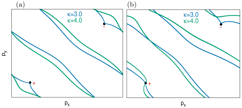
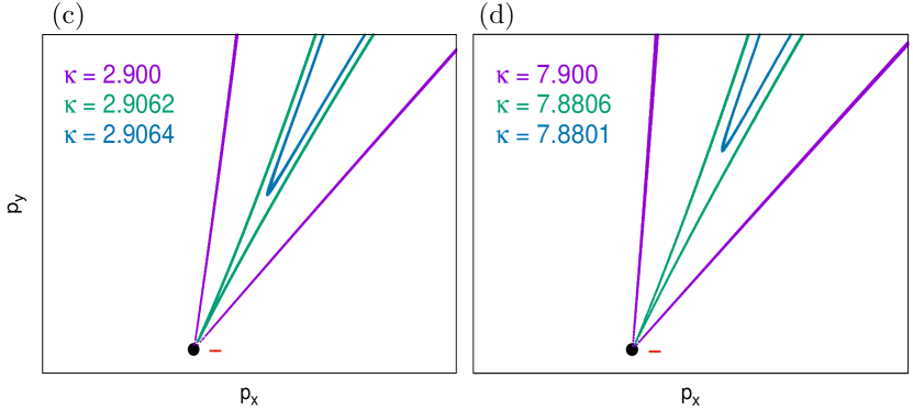
Figure 8: $n_{0}=2$: The reconstructed Fermi arcs (for $\kappa$ = 3 and 4) near the lift-off transitions without perturbations in (a) are compared with the reconstructed Fermi arcs after adding the symmetry breaking perturbations in (b). The parameters are given by $\delta V=V_{0}\sigma_{0}+V_{z}\sigma_{z}$, where $V_{0}=0.2$ and $V_{z}=0.3$. The other parameters are the same as in Figs. 4(d-f) and in Fig. 6. Note that symmetry of the Fermi arcs about both the diagonals $p_{x}=\pm p_{y}$ is broken in the perturbed case. Note also that the perturbed Fermi arcs get detached only from the -ve chiral WPP, but not from the +ve chiral WPP. (c) and (d) show the singular shapes of the Fermi arcs at and near the lift-off and re-attachment transitions, respectively, in the presence of the perturbation. It can be seen that the singular structure of the Fermi arc at and near the lift-off and re-attachment transitions remains intact.( See also Fig .6 for the unperturbed case.)

Here, we show that adding perturbations that break the symmetries of the $\kappa=0$ Hamiltonian do not change the results qualitatively. To see this, we consider a particular twist $n_{0}=2$ with overlapping Weyl point projections. Recall that for $V=\sum_{\mu=0}^{4}V_{\mu}\sigma^{\mu}$ the symmetries forced $V_{0},V_{z}=0$ and $V_{x},V_{y}$ real. We will break these symmetries by allowing for nonzero $V_{0},V_{z}$. For small couplings $\kappa<1$, the reconstructed Fermi arcs look very similar to those shown in Fig. 4(a). To check whether the lift-off and re-attachment transitions retain the singular shape of the Fermi arc close to the transitions, we study the reconstructed Fermi arcs, close to the transitions, with the symmetry breaking perturbations. The comparison with the earlier unperturbed results is shown in Fig. 8 and we find that the singular shape of the Fermi arc at and near the lift-off and re-attachment survices adding symmetry breaking perturbations to the tunnelling matrix. With the particular choice of $V_{\mu}$ we have made, the Fermi arc gets detached only from the negative chirality WPP, but remains attached to the positive chirality WPP. However, we have confirmed that various choices of $V_{\mu}$ can lead to detachment from either or both of the WPPs.

Appendix D Computation of Fermi Arc States at the Junction

In this section we will provide the details for the computation of the interface localized states. Our computation will closely follow Ref. Murthy2020, .

D.1 Surface states of the slabs

The idea is to look for decaying eigenstates into the bulk for both the slabs. Then we match solutions at the interface via the coupling term $H_{V}$ to get the interface localised states. Translational invariance is broken in the $z$-direction, but it remains unbroken in the transverse directions. The eigenstates can, hence, be labeled by the momenta $(k_{x},k_{y})$. We proceed with the following ansatz for the decaying eigenstates, -

$$\textrm{top slab:}\hskip 5.69046pt\ket{E,k_{x},k_{y}}^{t} =\sum_{n=0}^{\infty}\sum_{s}u_{t}^{n}{\bf\Phi}_{s}^{t}c^{\dagger}_{ns}\ket{0}$$ (38)

$$\textrm{bottom slab:}\hskip 5.69046pt\ket{E,k_{x},k_{y}}^{b} =\sum_{n=0}^{-\infty}\sum_{s}u_{b}^{-n}{\bf\Phi}_{s}^{b}c^{\dagger}_{ns}\ket{0}$$ (39)

where $|u_{\gamma}|<1$, for the state $\ket{E,k_{x},k_{y}}$ to be normalizable and $n$ is the discretised $z$ coordinate and here, ${\gamma}=(t,b)$. We then solve the Schrodinger equation, $H^{\gamma}\ket{E,k_{x},k_{y}}^{\gamma}=E\ket{E,k_{x},k_{y}}^{\gamma}$ to obtain $(u_{\gamma},\Phi^{\gamma}_{s})$. As shown in Ref. Murthy2020, , there are two normalizable solutions for $u_{\gamma}$ for a given $E$ and ${\bf k}=(k_{x},k_{y})$, which are given by

$$(u_{\gamma})_{\pm} =\frac{1}{2}(\xi_{\gamma}\pm\sqrt{\xi_{\gamma}^{2}-4}),$$ (40)

where, $\xi_{\gamma}$ is a solution of the following quadratic equation,

$$(1-t^{\prime 2})\xi_{\gamma}^{2}-4f_{1}^{\gamma}\xi_{\gamma}-E^{2}+4((f_{1}^{\gamma})^{2}+(f_{3}^{\gamma})^{2}+t^{\prime 2})=0.$$ (41)

For each root of $\xi_{\gamma}$, it is obvious from Eq. 40 that the two roots of $u_{\gamma}$ obey $(u_{\gamma})_{+}(u_{\gamma})_{-}=1$. This implies that one of the roots of $u_{\gamma}$ for each root of $\xi_{\gamma}$ must satisfy $|u_{\gamma}|\leqslant 1$. The equality holds only when $\xi_{\gamma}$ is real and $-2\leqslant\xi_{\gamma}\leqslant 2$. Therefore two roots of $\xi_{\gamma}$ give two solutions of $u_{\gamma}$ which give normalizable decaying eigenstates solutions for both slabs, only when $\xi_{\gamma}$ (which may be complex) lies outside the range $-2\leqslant\xi_{\gamma}\leqslant 2$.

A few further steps of algebra suffices to show that the spin wavefunctions ${\bf\Phi}^{\gamma}$ can be expressed as

$${\bf\Phi}^{t} =\left(1,\frac{-(2f^{t}_{3}-E)}{2f_{1}^{t}-(u_{t}+1/u_{t})+t^{\prime}(u_{t}-1/u_{t})}\right)^{T}$$ (42)

$${\bf\Phi}^{b} =\left(\frac{(2f^{b}_{3}+E)}{2f_{1}^{b}-(u_{b}+1/u_{b})+t^{\prime}(u_{b}-1/u_{b})},1\right)^{T}.$$ (43)

We can now construct a general wavefunction for the top slab as

$$\ket{\Psi^{t}({\bf k})}= \sum_{n=0}^{\infty}A_{1}^{t}({\bf k})(u_{1}^{t}({\bf k}))^{n}\Phi^{t}_{1}({\bf k})c^{\dagger}_{n}({\bf k})\ket{0}$$

$$\hskip 17.07182pt+A_{2}^{t}({\bf k})(u_{2}^{t}({\bf k}))^{n}\Phi^{t}_{2}({\bf k})c^{\dagger}_{n}({\bf k})\ket{0}$$

$$= \sum_{n=0}^{\infty}\psi^{t}_{n}({\bf k})c^{\dagger}_{n}({\bf k})\ket{0},$$ (44)

and for the bottom slab as

$$\ket{\Psi^{b}({\bf k})}= \sum_{n=0}^{-\infty}A_{1}^{b}({\bf k})(u_{1}^{b}({\bf k}))^{-n}\Phi^{b}_{1}({\bf k})c^{\dagger}_{n}({\bf k})\ket{0}$$

$$\hskip 17.07182pt+A_{2}^{b}({\bf k})(u_{2}^{b}({\bf k}))^{-n}\Phi^{b}_{2}({\bf k})c^{\dagger}_{n}({\bf k})\ket{0}$$

$$= \sum_{n=0}^{-\infty}\psi^{b}_{n}({\bf k})c^{\dagger}_{n}({\bf k})\ket{0},$$ (45)

where,

$$\psi^{t}_{n}({\bf k})= A_{1}^{t}({\bf k})(u_{1}^{t}({\bf k}))^{n}\Phi^{t}_{1}({\bf k})+A_{2}^{t}({\bf k})(u_{2}^{t}({\bf k}))^{n}\Phi^{t}_{2}({\bf k}),$$

$$\psi^{b}_{n}({\bf k})= A_{1}^{b}({\bf k})(u_{1}^{b}({\bf k}))^{-n}\Phi^{b}_{1}({\bf k})+A_{2}^{b}({\bf k})(u_{2}^{b}({\bf k}))^{-n}\Phi^{b}_{2}({\bf k}),$$ (46)

and $A_{1}^{\gamma}$, $A_{2}^{\gamma}$ are unknown constants. Next, our goal is to match the wavefunctions at the interface through the coupling term $H_{V}$ to fix the constants $A_{1}^{\gamma}$, $A_{2}^{\gamma}$.

D.2 Manipulation of coupling term $H_{V}$

Before proceeding further, we first need to write the coupling term $H_{V}$ in the transverse momentum space ${\bf k}=(k_{x},k_{y})$. On the interface, the true periodicity is that of superlattice. We label the operators which live on the zeroth layer of the top and bottom slabs by $\hskip 5.69046ptd_{\alpha s}({\bf R}),\hskip 5.69046pt\textrm{and}\hskip 5.69046ptf_{\alpha s}({\bf R})$ respectively, where the superlattice sites are given by ${\bf R}=m_{1}{\bf b_{1}}+m_{2}{\bf b_{2}}$, $m_{i}\in\mathbb{Z}$. Given a superlattice (SL) site, we then assign a ‘star’ of sites in both slabs as sublattice sites to this SL site with ‘$\alpha$’ representing the sublattice index. Writing the term $H_{V}$ in the SL index, we then get the following form from Eq. 7 in the. main paper,

$$H_{V}= \sum_{{\bf R},\alpha}\sum_{{\bf R^{\prime}},\beta}\{d^{\dagger}_{\alpha s}({\bf R})V_{ss^{\prime}}(|{\bf R-R^{\prime}}+{\boldsymbol{\delta}}_{\alpha}^{t}-{\boldsymbol{\delta}}_{\beta}^{b}|)f_{\beta s^{\prime}}({\bf R^{\prime}})$$

$$\hskip 56.9055pt+H.c\},$$ (47)

where we have used $c_{t0s}({\bf r}_{t})=c_{t0s}({\bf R}+{\boldsymbol{\delta}}^{t}_{\alpha})\equiv d_{\alpha s}({\bf R})$ and $c_{b0s}({\bf r}_{b})=c_{b0s}({\bf R}+{\boldsymbol{\delta}}^{b}_{\beta})\equiv f_{\beta s}({\bf R})$. We Fourier transform the operators,

$$d_{\alpha s}({\bf R})= \frac{1}{\sqrt{N_{SL}}}\sum_{{\bf p}\in BZ_{SL}}e^{i{\bf p.R}}\tilde{d}_{\alpha s}({\bf p})$$

$$f_{\beta s}({\bf R})= \frac{1}{\sqrt{N_{SL}}}\sum_{{\bf p}\in BZ_{SL}}e^{i{\bf p.R}}\tilde{f}_{\beta s}({\bf p}),$$ (48)

where $N_{SL}$ is total number of SL lattice sites and substitute these expressions in Eq. D.2, to get the following coupling term after simplification,

$$H_{V}= \sum_{{\bf p}\in BZ_{SL}}\sum_{\alpha\beta}\{\tilde{d}_{\alpha s}^{\dagger}({\bf p})\tilde{V}_{ss^{\prime}}^{\alpha\beta}({\bf p})\tilde{f}_{\beta s^{\prime}}({\bf p})+H.c\},$$ (49)

where

$$\tilde{V}_{ss^{\prime}}^{\alpha\beta}({\bf p})=\sum_{\bf R}e^{-i{\bf p.R}}V_{ss^{\prime}}({\bf R}+{\boldsymbol{\delta}}_{\alpha}^{t}-{\boldsymbol{\delta}}_{\beta}^{b}).$$ (50)

The ${\boldsymbol{\delta}}_{\alpha}^{t}$ and ${\boldsymbol{\delta}}_{\beta}^{b}$ are the relative position vectors of the sublattice sites with respect to the SL unit cell. Since the states $\ket{\Psi^{t}({\bf k})}$ (${\bf k}\in BZ_{t}$) and $\ket{\Psi^{b}({\bf k})}$ (${\bf k}\in BZ_{b}$) are defined where the operators $c_{ns}^{\dagger}({\bf k})$ act on the vacuum $\ket{0}$, we need to rewrite Eq. 49 in terms of the operators $c_{t0s}^{\dagger}({\bf k})$ and $c_{b0s}^{\dagger}({\bf k})$. So we want to relate the Fourier transforms of $d_{\alpha s}({\bf R})$ and $f_{\alpha s}({\bf R})$ with that of $c_{t0s}({\bf r}_{t})$ and $c_{b0s}({\bf r}_{b})$. We recall that

$$d_{\alpha s}({\bf R}) =c_{t0s}({\bf R}+\boldsymbol{\delta}_{\alpha}^{t})$$

$$=\frac{1}{\sqrt{N}}\sum_{{\bf k}\in BZ_{t}}e^{i{\bf k.(R}+\boldsymbol{\delta}_{\alpha}^{t})}c_{t0s}({\bf k})$$

$$=\frac{1}{\sqrt{N}}\sum_{{\bf p}\in BZ_{SL}}\sum_{l=1}^{N_{sc}/2}e^{i({\bf p+Q}_{l}).({\bf R}+\boldsymbol{\delta}_{\alpha}^{t})}c_{t0s}({\bf p+Q}_{l})$$

$$= \frac{1}{\sqrt{N_{SL}}}\sum_{{\bf p}\in BZ_{SL}}\frac{e^{i{\bf p.R}}}{\sqrt{N_{sc}/2}}\sum_{l=1}^{N_{sc}/2}e^{i({\bf p+Q}_{l}).\boldsymbol{\delta}_{\alpha}^{t}}c_{t0s}({\bf p+Q}_{l}).$$ (51)

In going from the second to the third step, we have used the fact that the momenta ${\bf k}\in BZ_{t}$ can be decomposed as: ${\bf k}_{l}={\bf p+Q}_{l}$, where ${\bf p}\in BZ_{SL}$ and ${\bf Q}_{l}=n_{1}{\bf g}_{1}+n_{2}{\bf g}_{2}$, $n_{i}\in\mathbb{Z}$. Since ${\bf g}_{1}$ and ${\bf g}_{2}$ are the reciprocal lattice vectors of the SL lattice, the following holds ${\bf Q}_{l}.{\bf R}=2\pi\times(integer)$. Here the label $l$ goes over the first and second Brillouin zones, since the SL BZ is $N_{sc}/2$ times smaller than the original BZ. From the third to the fourth step, we use the identity $e^{i{\bf Q}_{l}.{\bf R}}=1$ and write $N=N_{SL}\times N_{sc}/2$. Recall that the number of sites per SL unit cell is given by $N_{sc}=2\times(n_{0}^{2}+1)$ when $n_{0}$ is even and by $N_{sc}=(n_{0}^{2}+1)$ when $n_{0}$ is odd. In particular when $n_{0}=2$ (see Fig. 2 in the main paper), there are 5 sites of the top layer and 5 sites of the bottom layer per SL unit cell and a set of 5 values of ${\bf Q}_{l}=({\bf 0,g_{1},g_{2},-g_{1},-g_{2}})$. Comparing Eq. D.2 with the Eq. D.2, we get the following relations -

$$\tilde{d}_{\alpha s}({\bf p})=\frac{1}{\sqrt{N_{sc}/2}}\sum_{l=1}^{N_{sc}/2}e^{i({\bf p+Q}_{l}).\boldsymbol{\delta}_{\alpha}^{t}}c_{t0s}({\bf p+Q}_{l}).$$ (52)

and similarly for $\tilde{f}_{\beta s}({\bf p})$, we get

$$\tilde{f}_{\beta s}({\bf p})=\frac{1}{\sqrt{N_{sc}/2}}\sum_{l=1}^{N_{sc}/2}e^{i({\bf p+Q}_{l}).\boldsymbol{\delta}_{\beta}^{b}}c_{b0s}({\bf p+Q}_{l}).$$ (53)

Now substituting these expression of $\tilde{d}_{\alpha s}({\bf p})$ and $\tilde{f}_{\beta s}({\bf p})$ in Eq. 49, we finally get the following expression for the coupling term

$$H_{V}= \frac{1}{N_{sc}/2}\sum_{{\bf p}}\sum_{ss^{\prime}}\sum_{\alpha,\beta=0}^{N_{sc}/2-1}\hskip 5.69046pt\sum_{l,l^{\prime}=1}^{N_{sc}/2}\{e^{-i{\bf Q}_{l}.\boldsymbol{\delta}_{\alpha}^{t}+i{\bf Q}_{l^{\prime}}.\boldsymbol{\delta}_{\beta}^{b}}$$

$$\hskip 5.69046pt\times c^{\dagger}_{t0s}({\bf p+Q}_{l})\tilde{V}_{ss^{\prime}}^{\alpha\beta}({\bf p})c_{b0s^{\prime}}({\bf p+Q}_{l^{\prime}})+H.c\},$$ (54)

where $\tilde{V}_{ss^{\prime}}^{\alpha\beta}({\bf p})$ is given in Eq. 50.

D.3 Matching conditions

Since $\ket{\Psi^{t}({\bf k}_{l})}$ and $\ket{\Psi^{b}({\bf k}_{l})}$ are the eigenstates of $H^{t}$ and $H^{b}$ respectively and ${\bf k}_{l}={\bf p+Q}_{l}$, we can write the eigenstates of $H$ as $\ket{\Psi({\bf k}_{l})}=\ket{\Psi^{t}({\bf k}_{l})}+\ket{\Psi^{b}({\bf k}_{l})}$. Note that we have yet to determine the constants $A_{1}^{t},A_{2}^{t}$ and $A_{1}^{b},A_{2}^{b}$, defined in Eq. 46. Solving for $H\ket{\Psi({\bf k}_{l})}=E\ket{\Psi({\bf k}_{l})}$, gives us a discrete Schrodinger equation for a generic layer $n$ written as

$$h^{\gamma}_{nn}\psi_{n}^{\gamma}({\bf k}_{l})+h^{\gamma}_{n,n-1}\psi_{n-1}^{\gamma}({\bf k}_{l})+h^{\gamma}_{n,n+1}\psi_{n+1}^{\gamma}({\bf k}_{l})=E\psi_{n}^{\gamma}({\bf k}_{l})$$ (55)

where $\gamma=(t,b)$ and the different $h$ matrices are obtained from the Eqs. (3) and (4) in the main paper -

$$h^{\gamma}_{nn}={\bf M}^{\gamma},\hskip 8.5359pth^{\gamma}_{n,n+1}=-{\bf T}^{\dagger},\hskip 8.5359pth^{\gamma}_{n,n-1}=-{\bf T}.$$ (56)

(i) Next, let us consider $\gamma=t$ and $n=0$. Now when we solve $H\ket{\Psi({\bf k}_{l})}=E\ket{\Psi({\bf k}_{l})}$. In this case, the $n=-1$ layer does not exist and is instead replaced by the $n=0$ layer of the bottom slab. Hence, the coupling matrix $H_{V}$ will also act on the states $\ket{\Psi({\bf k}_{l})}$; this results in the following equation,

$$h^{t}_{00}\psi_{0}^{t}({\bf k}_{l})+\sum_{l^{\prime}}\tilde{h}(l,l^{\prime})\psi^{b}_{0}({\bf k}_{l^{\prime}})+h^{t}_{0,1}\psi_{1}^{t}({\bf k}_{l})=E\psi_{0}^{t}({\bf k}_{l}),$$ (57)

where the matrix $\tilde{h}(l,l^{\prime})$ is given by

$$\tilde{h}(l,l^{\prime})=\frac{\kappa}{N_{sc}/2}\sum_{\alpha\beta}e^{(-i{\bf Q}_{l}.\boldsymbol{\delta}_{\alpha}^{t}+i{\bf Q}_{l^{\prime}}.\boldsymbol{\delta}_{\beta}^{b})}V^{\alpha\beta}({\bf p}).$$ (58)

Eq. 55 remains valid even for $n=0$ (and setting $\gamma=t$), we get

$$h^{t}_{00}\psi_{0}^{t}({\bf k}_{l})+h^{t}_{0,-1}\psi_{-1}^{t}({\bf k}_{l})+h^{t}_{0,1}\psi_{1}^{t}({\bf k}_{l})=E\psi_{0}^{t}({\bf k}_{l}),$$ (59)

where $h^{t}_{0,-1}=-{\bf T}$. Now we can combine both Eq. 57 and Eq. 59 to finally get the wavefunction matching condition at the interface:

$$-{\bf T}\psi_{-1}^{t}({\bf k}_{l})+\sum_{l^{\prime}}\tilde{h}(l,l^{\prime})\psi^{b}_{0}({\bf k}_{l^{\prime}})=0.$$ (60)

(ii) Similarly we can consider $\gamma=b$ and $n=0$, and get the second matching condition at the interface:

$$-{\bf T}^{\dagger}\psi_{1}^{b}({\bf k}_{l})+\sum_{l^{\prime}}\tilde{h}^{\dagger}(l,l^{\prime})\psi^{t}_{0}({\bf k}_{l^{\prime}})=0.$$ (61)

Notice that in Eqs.60 and 61, each term is a $2\times 1$ column matrix. There are $N_{sc}/2$ number of different ${\bf k}_{l}={\bf p+Q}_{l}$ values. So each equation is essentially a set of $N_{sc}$ equations. Eqs.60 and 61 together give a set of $2\times N_{sc}$ equations and there are as many unknown constants ($A^{\gamma}_{1}({\bf k}_{l}),A^{\gamma}_{2}({\bf k}_{l})$) to be determined (see Eq. 46). We can combine Eq. 60 and Eq. 61 to give a single matrix equation,

$$M(E,\kappa,p_{x},p_{y})A=0,$$ (62)

where $A=(A^{t}_{1},A^{t}_{2},A^{b}_{1},A^{b}_{2})^{T}$ with,

$$A^{t}_{1} =(A^{t}_{1}(l_{1}),A^{t}_{1}(l_{2}),...A^{t}_{1}(l_{N_{sc}/2}))$$

$$A^{t}_{2} =(A^{t}_{2}(l_{1}),A^{t}_{2}(l_{2}),...A^{t}_{2}(l_{N_{sc}/2}))$$

$$A^{b}_{1} =(A^{b}_{1}(l_{1}),A^{b}_{1}(l_{2}),...A^{b}_{1}(l_{N_{sc}/2}))$$

$$A^{b}_{2} =(A^{t}_{2}(l_{1}),A^{t}_{2}(l_{2}),...A^{t}_{2}(l_{N_{sc}/2})).$$

Non trivial solutions for the constants lead to exponentially localised states at the interface, and for non trivial solutions to exist, we must have $\textrm{det}(M(E,\kappa,p_{x},p_{y}))=0$, for a given $E$ and $\kappa$. The determinant vanishing condition gives an equation, which $p_{x}$ and $p_{y}$ must satisfy for a given $(E,\kappa)$. The set of all such $(p_{x},p_{y})$, for $E=0$ and fixed $\kappa$, yields the reconstructed Fermi arc at the interface.

Appendix E Twists with $n_{0}=4$ and $n_{0}=5$

We have already discussed the results for a non trivial twist with $n_{0}=2$ for both the cases of overlapping and non overlapping WPPs in detail in the main text. Here, for completeness, we consider higher values of $n_{0}$. First, we clarify that the case for $n_{0}=3$ has not been studied here in detail, because it is very similar to the case with $n_{0}=2$ - in both cases, their superlattices are similar - the SL unit cell contains the same number of lattice sites $N_{sc}=10$ and the unit cell is $N_{sc}/2=5$ times larger than the original unit cell. So we discuss below, the cases when $n_{0}=4$ and $n_{0}=5$.

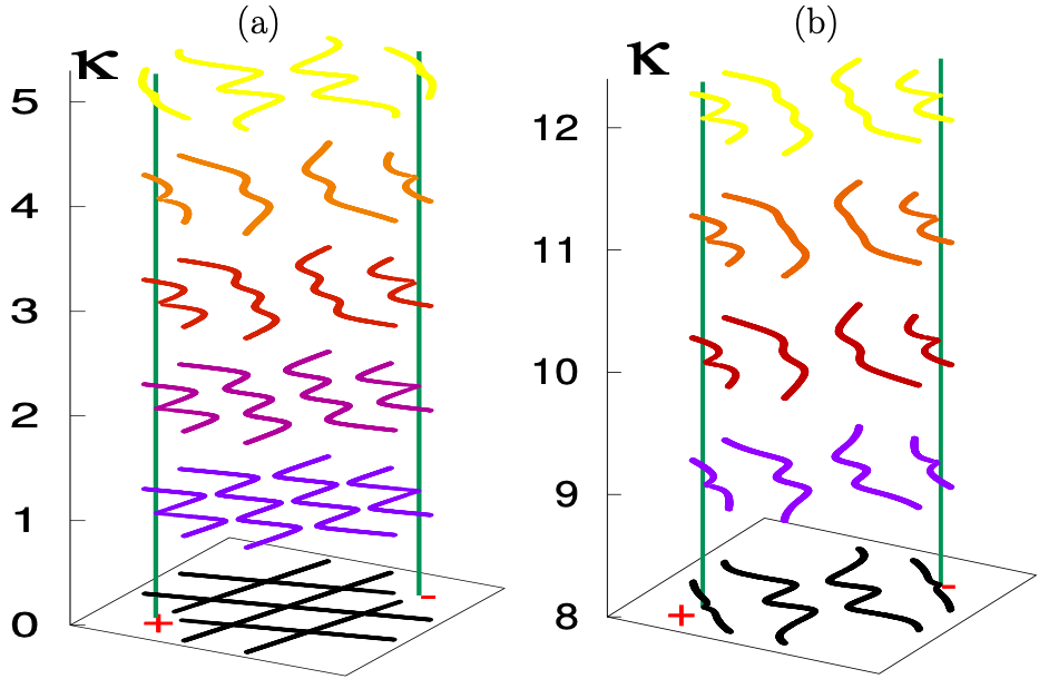
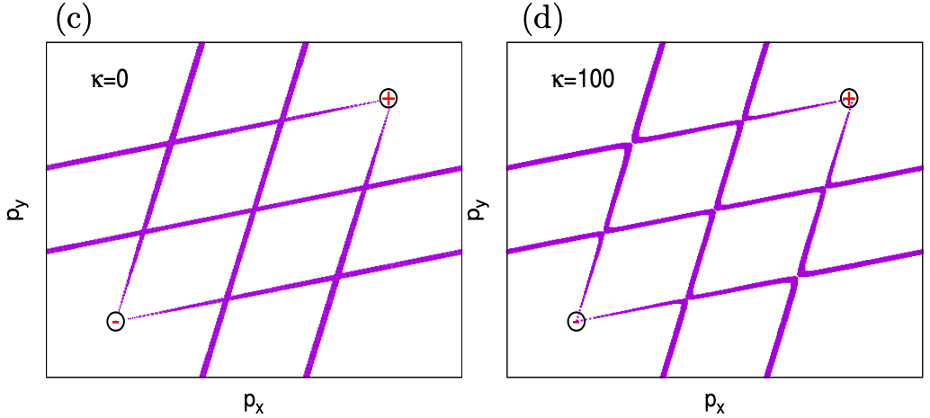
Figure 9: $n_{0}=4$ with overlapping Weyl point projections in the surface BZ. In (a) and (b), reconstructed Fermi arcs are shown for couplings in the ranges $\kappa=(0,5)$ and $\kappa=(8,12)$ respectively. The detachment of the FAs from the WPPs and its subsequent reattachment occur in the coupling range $\kappa=(5,7)$. This region of $\kappa$ is explored separately in Fig.6. Parameters taken are $t^{\prime}=1.5$ and $V_{x}=1,V_{y}=0$. The duality between the strong and weak coupling in the FA reconstruction is shown in (c) and (d).

E.1 Twist with ${\bf n_{0}=4}$

Here, we shall consider the twist with $n_{0}=4$ for the case when the WPPs overlap. We start with a system with the slabs aligned and the Fermi arcs lying along the $x$-axis. Then the top slab is given a twist by an angle $\theta_{4}=\tan^{-1}(1/4)$ counterclockwise and the bottom slab is twisted counterclockwise by the angle $(\pi/2-\theta_{4})$, such that the site $(4,-1)$ of top layer lies on top of the site $(1,-4)$ of the bottom layer. We choose $k_{0}=2\pi/3$ so that the positively charged chiral WPP of the top slab lies on the positively charged chiral WPP of the bottom slab and the negatively charged chiral WPPs also lie on top of each other. The overlapping occurs in the first SL BZ after translating the WPPs by the appropriate reciprocal lattice vectors of the SL.

The reconstructed Fermi arc is shown in Fig. 9. As in the $n_{0}=2$ case, we find a duality in the Fermi arc reconstruction between strong and weak inter-layer coupling strengths. There is also a regime of parameters where the Fermi arc is detached from the WPPs. The Fermi arc detachment occurs at around $\kappa\sim 5$ and then it again re-attaches at $\kappa\sim 7$. This is depicted in Fig. 10.

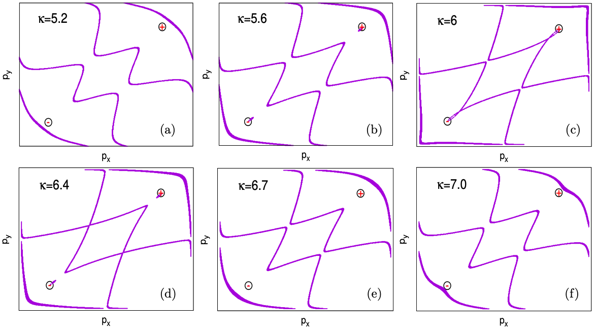
Figure 10: The surface BZ for $n_{0}=4$ in the coupling range $\kappa=(5.2,7.0)$ is explored, where the FA detaches from the WPPs and then reattaches again.

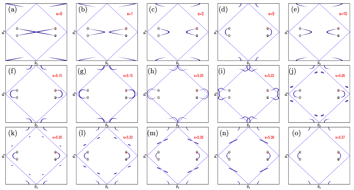
Figure 11: $n_{0}=5$: The panels show the evolution of the reconstructed Fermi arcs with the coupling strength $\kappa$. The parameters are $k_{0}=\pi/4$, $t^{\prime}=0.8$, $V_{x}=1,V_{y}=0$. The inscribed blue square is the boundary of the superlattice BZ. The Weyl point projections of the top (bottom) slab are in red (black) colour. In the first row, the reconstructed Fermi arcs are shown for $\kappa=0,1,3,5$ and 10. Notice the sign change of curvature of Fermi arc for $\kappa=5$. In the second and third rows, the Fermi arc reconstruction around the coupling $\kappa=5$ has been explored in more detail. In the second row, as $\kappa$ is increased from 5, the Fermi arc deforms and at around $\kappa=5.26$, it splits to produce a pair of extra small closed loops which are inside the first superlattice BZ. In the third row with increasing $\kappa$, the extra small closed loops move towards the boundary of the superlattice BZ and merge with the another small loop coming from outside the first superlattice BZ. Finally they disappear at $\kappa=5.37$, leaving only those Fermi arcs which are attached to the WPPs. At larger couplings, the reconstructed Fermi arcs are similar to the small coupling results (e.g. figure (c) and (e) ), as expected from the duality between strong and weak couplings.

E.2 Twist with ${\bf n_{0}=5}$

The first non trivial case with $n_{0}$ odd is when $n_{0}=5$. Here we consider the Fermi arc reconstruction for the case of non overlapping WPPs. We rotate the top slab counterclockwise and the bottom slab clockwise until the lattice site $(5,-1)$ of the top layer and the site $(5,1)$ of the bottom layer lie on top of each other. Here the angle of rotation is $\theta_{5}=\tan^{-1}(1/5)$. We take $k_{0}=\pi/4$. The Weyl point projections of positive and negative chirality are now at $k_{0}(\cos{\theta_{5}},\pm\sin{\theta_{5}})$ and $k_{0}(-\cos{\theta_{5}},\mp\sin{\theta_{5}})$ respectively, where the upper (lower) sign is for the top (bottom) slab. The reconstructed Fermi arcs are shown in Fig. 11. At zero coupling, there are unreconstructed Fermi arcs of the individual slabs. As we switch on and increase the coupling, the reconstructed Fermi arcs change their signs of curvature at around $\kappa=5$ (see Fig. 11(c) and Fig. 11(d) ). The Fermi arcs deform and split when the coupling is increased slowly beyond $\kappa=5$. After splitting, a pair of small closed loops are formed. The small closed loops approach the superlattice BZ boundary and finally disappear after merging. An almost similar feature exists also for the $n_{0}=2$ case, where newly formed extra small loops disappear after merging at the superlattice BZ boundary (see Fig. 4(c)).

References

- (1) S. Murakami, New J. Phys. 9, 356 (2007).
- (2) X. Wan, A. M. Turner, A. Vishwanath and S. Y. Savrasov, Phys. Rev. B 83, 205101 (2011); P. Hosur, S. A. Parameswaran and A. Vishwanath, Phys. Rev. Lett. 108, 046602 (2012).
- (3) K. Y. Yang, Y. M. Lu and Y. Ran, Phys. Rev. B84, 075129 (2011).
- (4) A. A. Burkov and L. Balents, Phys. Rev. Lett. 107, 127205 (2011).
- (5) G. Xu, H. Weng, Z. Wang, X. Dai and Z. Fang, Phys. Rev. Lett. 107, 186806 (2011).
- (6) S.-Y. Xu, I. Belopolski, N. Alidoust, M. Neupane, G. Bian, C. Zhang, R. Sankar, G. Chang, Z. Yuan, C.-C. Lee, S.-M. Huang, H. Zheng, J. Ma, D. S. Sanchez, B. Wang, A. Bansil, F. Chou, P. P. Shibayev, H. Lin, S. Jia, and M. Z. Hasan, Science 349, 613 (2015); S.-Y. Xu, N. Alidoust, I. Belopolski, Z. Yuan, G. Bian, T.-R. Chang, H. Zheng, V. N. Strocov, D. S. Sanchez, G. Chang, C. Zhang, D. Mou, Y. Wu, L. Huang, C.-C. Lee, S.-M. Huang, B. Wang, A. Bansil, H.-T. Jeng, T. Neupert, A. Kaminski, H. Lin, S. Jia and M. Z. Hasan, Nat. Phys. 11, 748 (2015).
- (7) B. Q. Lv, H. M. Weng, B. B. Fu, X. P. Wang, H. Miao, J. Ma, P. Richard, X. C. Huang, L. X. Zhao, G. F. Chen, Z. Fang, X. Dai, T. Qian and H. Ding, Phys. Rev. X 5, 031013 (2015); B. Q. Lv, N. Xu, H. M. Weng, J. Z. Ma, P. Richard, X. C. Huang, L. X. Zhao, G. F. Chen, C. E. Matt, F. Bisti, V. N. Strocov, J. Mesot, Z. Fang, X. Dai, T. Qian, M. Shi and H. Ding, Nat. Phys. 11, 724 (2015).
- (8) L. Lu, Z. Wang, D. Ye, L. Ran, L. Fu, J. D. Joannopoulos and M. Soljacic, Science 349, 622 (2015).
- (9) A. C. Potter, I. Kimchi, and A. Vishwanath, Nature Communications 5, 5161 (2014).
- (10) P. J. W. Moll, N. L. Nair, T. Helm, A. C. Potter, I. Kimchi, A. Vishwanath, and J. G. Analytis, Nature 535, 266 (2016).
- (11) For a review, see A. H. Castro Neto, F. Guinea, N. M. R. Peres, K. S. Novoselov and A. K. Geim, Rev. Mod. Phys. 81, 109 (209).
- (12) D. T. Son and B. Z. Spivak, Phys. Rev. B88, 104412 (2013).
- (13) S. A. Yang, H. Pan and F. Zhang, Phys. Rev. Lett. 115, 156603 (2015).
- (14) S. Nandy, G. Sharma, A. Taraphder and S. Tewari, Phys. Rev. Lett. 119, 176804 (2017).
- (15) S. Ueda, T. Habe and Y. Asano, J. Phys. Soc. Jpn 83, 014701 (2014).
- (16) N. Bovenzi, M. Breitkreiz, P. Baireuther, T. E. O’Brien, J. Tworzydlo, I. Adagideli, and C. W. J. Beenakker, Phys. Rev. B96, 035437 (2017).
- (17) U. Khanna, D. K. Mukherjee, A. Kundu and S.Rao, Phys. Rev. B93 121409(R) (2016); K.A. Madsen, E. J. Bergholtz and P. W. Brouwer, Phys. Rev. B95, 064511 (2017).
- (18) U. Khanna, S.Rao and A.Kundu, Phys. Rev. B95, 201115(R), 2017).
- (19) D. K. Mukherjee, S. Rao and A. Kundu, Phys. Rev. B96, 161408(R) (2017).
- (20) D. K. Mukherjee, S. Rao and S. Das, J. Phys. Condens. Matter 31, 045302 (2019).
- (21) D. Sinha and K. Sengupta, Phys. Rev. B99, 075153 (2019).
- (22) Y. Baum, E. Berg, S. A. Parameswaran, and A. Stern, Phys. Rev. X 5, 041046 (2015).
- (23) C. M. Wang, H.-P. Sun, H.-Z. Lu, and X. C. Xie, Phys. Rev. Lett. 119, 136806 (2017); C. Zhang, Y. Zhang, X. Yuan, S. Lu, J, Zhang, A. Narayan, Y. Liu, H. Zhang, Z. Ni, R. Kiu, E. S. Choim A. Suslov, S. Sanvito, L. Pi, H.-Z. Lu, A. C. Potter and F. Xiu, Nature 565, 331 (2019).
- (24) O. Deb and D. Sen, Phys. Rev. B 95, 144311 (2017).
- (25) T. M. McCormick, S. J. Watzman, J. P. Heremans and N. Trivedi, Phys. Rev. B97, 195152 (2018).
- (26) K. S. Novoselov, A. Mishchenko, A. Carvalho, and A. H. Castro Neto, Science 353 (2016).
- (27) D. L. Duong, S. J. Yun, and Y. H. Lee, ACS Nano 11, 11803 (2017).
- (28) E. J. Mele, Phys. Rev. B81, 161405(R) (2010).
- (29) E. J. Mele, Phys. Rev. B84, 235439 (2011).
- (30) R. Bistritzer and A. H. MacDonald, Proc. Nat. Acad. Sci. USA 108, 12233 (2011).
- (31) P. San-Jose, J. Gonzalez, and F. Guinea, Phys. Rev. Lett. 108, 216802 (2012).
- (32) V. Dwivedi, Phys. Rev. B97, 064201 (2018).
- (33) H. Ishida and A. Liebsch, Phys. Rev. B98, 195426 (2018).
- (34) G. Murthy, H. A. Fertig, and E. Shimshoni, Phys. Rev. Research 2, 013367(2020).
- (35) See appendix for further details.
- (36) E. Fradkin, Phys. Rev. B33, 3263 (1986); P. Goswami and S. Chakravarty, Phys. Rev. Lett. 107, 196803 (2011); A. Altland and D. Bagrets, Phys. Rev. Lett. 114, 257201 (2015); B. Roy, R.-J. Slager and V. Juricic, Phys. Rev. X8, 031076 (2018).
- (37) R. Nandkishore, D. A. Huse, and S. L. Sondhi, Phys. Rev. B89, 245110 (2014); J. H. Pixley, D. A. Huse, and S. Das Sarma, prx 6 021042 (2016); J. H. Pixley, D. A. Huse, and S. Das Sarma, Phys. Rev. B94, 121107(R) (2016); J. H. Pixley, Y.-Z. Chou, P. Goswami, D. A. Huse, R. Nandkishore, L. Radzihovsky, and S. Das Sarma, Phys. Rev. B95, 235101 (2017); J. H. Wilson, J. H. Pixley, P. Goswami, and S. Das Sarma, Phys. Rev. B95, 155122 (2017).
- (38) E. V. Gorbar, V. A. Miransky, I. A. Shovkovy, and P. O. Sukhachov, Phys. Rev. B93, 235127 (2016); R.-J. Slager, V. Juricic, and B. Roy, Phys. Rev. B96, 201401(R) (2017).
- (39) J. H. Wilson, J. H. Pixley, D. A. Huse, G. Refael, and S. Das Sarma, Phys. Rev. B97, 235108 (2018).