Constraints on the time variation of the speed of light using Pantheon dataset

Abstract

Both the absolute magnitude of type Ia supernovae (SNe Ia) and the luminosity distance of them are modified in the context of the minimally extended varying speed of light (meVSL) model compared to those of general relativity (GR). We have analyzed the likelihood of various dark energy models under meVSL by using the Pantheon SNe Ia data. Both $\omega$CDM and CPL parameterization dark energy models indicate a cosmic variation of the speed of light at the 1-$\sigma$ level. For $\Omega_{\text{m}0}=0.30,0.31$, and 0.32 with $(\omega_{0}\,,\omega_{a})=(-1\,,0)$, 1-$\sigma$ range of $\dot{\tilde{c}}_{0}/\tilde{c}_{0}\,(10^{-13}\,\text{yr}^{-1})$ are (-8.76  , -0.89), (-11.8  , 3.93), and (-14.8  , -6.98), respectively. Meanwhile, 1-$\sigma$ range of $\dot{\tilde{c}}_{0}/\tilde{c}_{0}(10^{-12}\,\text{yr}^{-1})$ for CPL dark energy models with $-1.05\leq\omega_{0}\leq-0.95$ and $0.28\leq\Omega_{\text{m}0}\leq 0.32$, are (-6.31 , -2.98). The value of $\tilde{c}$ at $z=3$ can be larger than that of the present by $0.2\sim 3$ % for $\omega$CDM models and $5\sim 13$ % for CPL models. We also obtain $-25.6\leq\dot{\tilde{G}}_{0}/\tilde{G}_{0}\,(10^{-12}\,\text{yr}^{-1})\leq-0.36$ for viable models except for CPL model for $\Omega_{\text{m}0}=0.28$. We obtain the increasing rate of the gravitational constant as $1.65\leq\dot{\tilde{G}}_{0}/\tilde{G}_{0}\,(10^{-12}\,\text{yr}^{-1})\leq 3.79$ for that model.

I Introduction

It is free to choose a local value of the speed of light, $𝑐$ because that only implies a rescaling of the units of length. However, as long as the local value of $c$ is a constant at the constant time hypersurface, then it can satisfy both special relativity and general relativity. Thus, the time variational of the speed of light is physically meaningful in this model. Various models of the cosmological variable speed of light have sometimes been invoked in order to explain problematic observations. In addition, Newton’s gravitational constant, $G$, could in principle be variable. In order to avoid trivial rescaling of units, one must test the simultaneous variation of $c$, $G$, and maybe the fine structure constant $\alpha$ which can be combined to a dimensionless number. Note that functions of $c$ and $G$ as a redshift $z$ are given in meVSL model Lee:2020zts .

The Pantheon compilation of a total of 1048 SNe Ia ranging from $0.01<z<2.3$ consists of 365 spectroscopically confirmed SNe Ia discovered by the Pan-STARRS1 (PS1) Medium Deep Survey combined with the subset of 279 PS1 SNe Ia ($0.03<z<0.68$) with useful distance estimates of SN Ia from SDSS, SNLS, various low-z and HST samples Scolnic:2017caz . Cosmological models fitted over to minimize the $\chi^{2}$ for flat $\Lambda$CDM and $\omega$CDM models without systematic uncertainties on $\Omega_{\text{m}0}$ give $0.284\pm 0.012$ and $0.350\pm 0.035$, respectively. The 1-$\sigma$ constrain on $\omega$ for $\omega$CDM model is $-1.251\pm 0.144$. The Pantheon dataset provides to precisely constrain to about 10 % on $\Omega_{\text{m}0}$ and 12 % on $\omega$ for flat $\omega$CDM model and to 4 % on $\Omega_{\text{m}0}$ for the flat $\Lambda$CDM model.

We briefly review meVSL model and luminosity distance of this model in section II. We analyze the bounds on the variation of $\tilde{c}$ and that of $\tilde{G}$ by using the Pantheon data for various dark energy models in section III. Summary and conclusions are given in Sec. IV.

II Review on meVSL

The four-dimensional spacetime of spatially homogeneous and isotropic, expanding universe can be regarded as a contiguous bundle of homogeneous and isotropic spatial constant time hypersurfaces whose length scale evolves in time. The metric of this spacetime known as Friedmann-Lemaître-Robertson-Walker (FLRW) universe can be written as

$$ds^{2}=-\tilde{c}^{2}dt^{2}+a^{2}(t)\gamma_{ij}dx^{i}dx^{j}=-\tilde{c}^{2}dt^{2}+a^{2}(t)\left(\frac{dr^{2}}{1-kr^{2}}+r^{2}d\Omega^{2}\right)=-\tilde{c}^{2}dt^{2}+a^{2}(t)\left[d\chi^{2}+f_{k}^{2}(\chi)d\Omega^{2}\right]\,,$$ (1)

where $\gamma_{ij}(\vec{x})$ is a time-independent spatial metric defined on the hypersurface, and $a(t)$ is the scale factor that relates the physical distance to the comoving distance. We also define $\chi=D_{\text{c}}$ is the comoving distance defined as

$$D_{\text{C}}(z)\equiv\int_{0}^{r}\frac{dr^{\prime}}{\sqrt{1-kr^{2}}}=\frac{\tilde{c}_{0}}{H_{0}}\int_{0}^{z}\frac{dz^{\prime}}{E^{(\text{GR})}(z^{\prime})}\equiv\frac{\tilde{c}_{0}}{H_{0}}d_{\text{C}}(z)\,,$$ (2)

and $f_{k}(\chi)=\sinh(\sqrt{-k}\chi)/\sqrt{-k}=D_{\text{M}}$ is the transverse comoving distance given as

$$D_{\text{M}}(z)=D_{\text{M}}^{(\text{GR})}(z)=\begin{cases}\frac{\tilde{c}_{0}}{H_{0}}\frac{1}{\sqrt{\Omega_{K0}}}\sinh\left(\sqrt{\Omega_{k0}}\frac{H_{0}}{\tilde{c}_{0}}D_{\text{C}}\right)&\Omega_{k0}>0\\ D_{\text{C}}&\Omega_{k0}=0\\ \frac{\tilde{c}_{0}}{H_{0}}\frac{1}{\sqrt{|\Omega_{K0}|}}\sin\left(\sqrt{|\Omega_{k0}|}\frac{H_{0}}{\tilde{c}_{0}}D_{\text{C}}\right)&\Omega_{k0}<0\end{cases}\,,$$ (3)

where the present values of the speed of light and the that of the Hubble parameter are $\tilde{c}_{0}=2.9979\times 10^{5}$ km/s and $H_{0}=100h$ km/Mpc/s. The timelike worldlines of constant space define the threading, while the spacelike hypersurface of constant time defines the slicing to the four-dimensional spacetime. Each spacelike threading corresponds to a homogeneous universe and the slicing is orthogonal to these universes. One can define the constant physical quantities - the density, the temperature, and the speed of light - on each spacelike hypersurface. Thus, our choice of coordinates was natural and we did not need to consider alternatives. Ricci tensors and Ricci scalar curvature are obtained from the given metric in Eq. (1) Lee:2020zts

$$\tilde{R}_{00}=-\frac{3}{\tilde{c}^{2}}\left(\frac{\ddot{a}}{a}-H^{2}\frac{d\ln\tilde{c}}{d\ln a}\right)\quad,\quad\tilde{R}_{ii}=\frac{g_{ii}}{\tilde{c}^{2}}\left(2\frac{\dot{a}^{2}}{a^{2}}+\frac{\ddot{a}}{a}+2k\frac{\tilde{c}^{2}}{a^{2}}-H^{2}\frac{d\ln\tilde{c}}{d\ln a}\right)\,,$$ (4)

$$\tilde{R}=\frac{6}{\tilde{c}^{2}}\left(\frac{\ddot{a}}{a}+\frac{\dot{a}^{2}}{a^{2}}+k\frac{\tilde{c}^{2}}{a^{2}}-H^{2}\frac{d\ln\tilde{c}}{d\ln a}\right)\,.$$ (5)

The energy-momentum tensor of the $i$-th perfect fluid with the equation of state $\omega_{i}$ is given by Lee:2020zts

$$T_{(i)\mu}^{\nu}=\text{diag}\left(-\rho_{i}\tilde{c}^{2},P_{i},P_{i},P_{i}\right)\quad,\,\text{with}\quad\rho_{i}\tilde{c}^{2}=\rho_{i0}\tilde{c}_{0}^{2}a^{-3(1+\omega_{i})}\,,$$ (6)

where $\tilde{c}_{0}$ is the present value of the speed of light, $\rho_{i0}$ is the present value of mass density of the i-component, and we use $a_{0}=1$.

One can derive Einstein’s field equations including the cosmological constant from Eqs. (4)-(6)

$$\frac{\dot{a}^{2}}{a^{2}}+k\frac{\tilde{c}^{2}}{a^{2}}-\frac{\Lambda\tilde{c}^{2}}{3}=\frac{8\pi\tilde{G}}{3}\sum_{i}\rho_{i}\,,$$ (7)

$$\frac{\dot{a}^{2}}{a^{2}}+2\frac{\ddot{a}}{a}+k\frac{\tilde{c}^{2}}{a^{2}}-\Lambda\tilde{c}^{2}-2H^{2}\frac{d\ln\tilde{c}}{d\ln a}=-8\pi\tilde{G}\sum_{i}\frac{P_{i}}{\tilde{c}^{2}}=-8\pi\tilde{G}\sum_{i}\omega_{i}\rho_{i}\,,$$ (8)

$$\frac{\ddot{a}}{a}=-\frac{4\pi\tilde{G}}{3}\sum_{i}\left(1+3\omega_{i}\right)\rho_{i}+\frac{\Lambda\tilde{c}^{2}}{3}+H^{2}\frac{d\ln\tilde{c}}{d\ln a}\,.$$ (9)

II.1 Luminosity distance

The distance modulus $\mu=m-M$ is the difference between the apparent magnitude $m$ (ideally, corrected from the effects of interstellar absorption) and the absolute magnitude $M$ of an astronomical object. It is related to the luminosity distance $D_{L}$ in parsecs by

$$\mu=5\log_{10}\left[\frac{D_{\text{L}}}{1\text{Mpc}}\right]+25\,.$$ (10)

This definition is convenient because the observed brightness of a light source is related to its distance by the inverse square law and because brightnesses are usually expressed not directly, but in magnitudes. Absolute magnitude $M$ is defined as the apparent magnitude of an object when seen at a distance of $10$ parsecs. The magnitudes and flux, $F$ are related by

$$m=-2.5\log_{10}F(D_{\text{L}})\quad,\quad M=-2.5\log_{10}F(10)\,.$$ (11)

The so-called Chevallier-Polarski-Linder (CPL) parametrization, which takes $\omega$ to be a linear function of the scale factor $a$, is given by Chevallier:2000qy ; Linder:2002et

$$\omega=\omega_{0}+(1-a)\omega_{a}\,.$$ (12)

$E^{(\text{GR})}$ in the Eq. (2) for the flat Universe by using CPL parametrization is given by

$$E^{(\text{GR})}=\sqrt{\Omega_{\text{m}0}a^{-3}+\left(1-\Omega_{\text{m}0}\right)a^{-3(1+\omega_{0}+\omega_{a})}e^{-3\omega_{a}(1-a)}}\,.$$ (13)

In order to obtain the luminosity distance in the meVSL model, one needs to re-examine it from its definition. We define the observed luminosity as $L_{0}$ detected at the present epoch, which is different from the absolute luminosity $L_{s}$ of the source emitted at the redshift $z$. We can write the conservation of flux $\mathcal{F}$ from the source point to the observed point as

$$\mathcal{F}=\frac{L_{s}}{4\pi D_{\text{L}}^{2}(z)}=\frac{L_{0}}{4\pi D_{\text{M}}^{2}(z_{0})}\,.$$ (14)

The absolute luminosity, $L_{s}\equiv\Delta E_{1}/\Delta t_{1}$ is defined by the ratio of the energy of the emitted light $\Delta E_{1}$ to the time-interval of that emission $\Delta t_{1}$. And the observed luminosity also can be written as, $L_{0}=\Delta E_{0}/\Delta t_{0}$. Thus, one can rewrite the luminosity distance by using Eq. (14) as

$$D_{\text{L}}^{2}(z)=\frac{L_{s}}{L_{0}}D_{\text{M}}^{2}(z_{0})=\frac{\Delta E_{1}}{\Delta E_{0}}\frac{\Delta t_{0}}{\Delta t_{1}}D_{\text{M}}^{2}(z_{0})=\left(1+z\right)^{2-\frac{b}{4}}D_{\text{M}}^{2}(z_{0})\,,$$ (15)

where we use

$$\frac{\Delta E_{1}}{\Delta E_{0}} =\frac{\tilde{h}_{1}\tilde{\nu}_{1}}{\tilde{h}_{0}\tilde{\nu}_{0}}=\frac{\tilde{\nu}_{1}^{(\text{GR})}}{\tilde{\nu}_{0}^{(\text{GR})}}=(1+z)\quad,\quad\frac{\Delta t_{0}}{\Delta t_{1}}=\frac{\tilde{\nu}_{1}}{\tilde{\nu}_{0}}=\frac{\tilde{\nu}_{1}^{(\text{GR})}(1+z)^{-b/4}}{\tilde{\nu}_{0}^{(\text{GR})}}=(1+z)^{1-\frac{b}{4}}\,.$$ (16)

Thus, we obtain the relation between the luminosity distance and the transverse comoving distance in meVSL (also for the angular diameter distance, $D_{\text{A}}$)

$$D_{\text{L}}(z)=\left(1+z\right)^{1-\frac{b}{8}}D_{\text{M}}(z)=\left(1+z\right)^{2-\frac{b}{8}}D_{\text{A}}(z)\,.$$ (17)

This is the cosmic distance duality relation (CDDR) of the meVSL model and can be rewritten as

$$\frac{(1+z)^{2}D_{\text{A}}}{D_{\text{L}}}=(1+z)^{\frac{b}{8}}\,.$$ (18)

Under this assumption, we have the modification of the absolute magnitude of SNe Ia

$$\text{M}-\text{M}_{0}=-2.5\log\left[\frac{L}{L_{0}}\right]=\frac{5}{4}b\log\left[a\right]\,,$$ (19)

where the subscript $0$ refers to the local value of $M$. Thus, the distance module of meVSL, $\mu\equiv m-M$ is written by

$$\mu(z) =m-\text{M}=5\log_{10}\left[\frac{D_{\text{L}}}{\text{Mpc}}\right]+25\quad,\quad D_{\text{M}}=\frac{\tilde{c}_{0}}{H_{0}}d_{\text{L}}(z)\,\,,\,\,d_{\text{L}}(z)\equiv\int_{0}^{z}\frac{dz^{\prime}}{E^{(\text{GR})}(z^{\prime})}\,.$$ (20)

The theoretically predicted apparent magnitude $m_{\text{th}}$ is given by

$$m_{\text{th}}(z) =M+5\log\left[\frac{D_{\text{L}}}{1\text{Mpc}}\right]+25+\frac{5}{4}b\log\left[a\right]=M+42.3841+5\log\left[\frac{d_{\text{L}}}{h(1+z)^{b/4}}\right]\,.$$ (21)

II.2 Analysis

The chi-squared is a weighted sum of squared deviations

$$\chi^{2}=\sum_{i,j}\left(m_{i,\text{obs}}-m_{i,\text{th}}\right)C^{-1}_{ij}\left(m_{i,\text{obs}}-m_{j,\text{th}}\right)\,,$$ (22)

where $m_{i,\text{obs}}$ is the observational apparent magnitude, and $m_{i,\text{th}}$ is the theoretical apparent magnitude of SNe Ia at the redshift $z_{i}$ given in Eq. (20), and $C_{ij}=D_{ij}+C_{\text{sys}}$ is the covariance matrix where $D_{ij}=\sigma_{i}^{2}\delta_{ij}$ is the variance of each observation and $C_{\text{sys}}$ is a non-diagonal matrix associated with the systematic uncertainties. The reduced chi-square statistic defined as chi-square per degree of freedom is used extensively in the goodness of fit testing

$$\chi^{2}_{\nu}=\frac{\chi^{2}}{\nu}\,,$$ (23)

where the degree of freedom, $\nu=N-p$, equals the number of observations $N$ minus the number of fitted parameters $p$. As a rule of thumb, when the variance of the measurement error is known a priori, a $\chi_{\nu}^{2}\gg 1$ indicates a poor model fit. A $\chi_{\nu}^{2}>1$ indicates that the fit has not fully captured the data (or that the error variance has been underestimated). In principle, a value of $\chi_{\nu}^{2}$ around $1$ indicates that the extent of the match between observations and estimates is in accord with the error variance.

III A bound for the variation of $c$

The previously known bound for the temporal variation of $c$ is obtained from the variation of the radius of a planet Racker:2007hj . However, this bound is based on the analysis of the time variation of the radius of Mercury McElhinny:1978na by using the special model so-called a covariant variable speed of light theory proposed by Magueijo Magueijo:2000zt . Thus, this bound cannot be used in the meVSL model. One uses SNIa as standard candles to probe the cosmic expansion rate of the late Universe. We investigate the time variation of the speed of light by using the Pantheon type Ia supernova (SNIa) data Scolnic:2017caz . We investigate two main models, $\omega$CDM (i.e., constant $\omega$) and CPL dark energy models.

III.1 $\tilde{c}$ for $\omega$CDM

We probe the so-called $\omega$CDM models which are $\omega_{a}=0$ in Eq. (12). We analyze various models for different values of cosmological parameters by using a maximum likelihood analysis. The results of these models have summarized in table. 1. Interesting features of relationships between cosmological parameters can be found in this table. For the fixed value of $\omega_{0}$, both $M_{0}$ and $h$ are degenerated and so are $\Omega_{m0}$ and $b$. Thus, we obtain almost the same values of $M_{0}$ and $h$ if we fix $\Omega_{m0}$ and only $b$-values are changed. On the other hand, if we fix the $h$-value, then only $M_{0}$ values are changed from these fixed values of $h$ and both $\Omega_{m0}$ and $b$ are irrelevant for $h$-values. As we show below, the only $\omega$CDM models which provide the time variations of the speed of light from Pantheon data are obtained when $\omega_{0}=-1$ and $0.30\leq\Omega_{m0}$.

Table 1: Best fit values and their 1-$\sigma$ errors of cosmological parameters for $\omega$CDM models (i.e., $\omega_{a}=0$). The time variation of the speed of light is possible for green color indicated models.

Models	Submodels	$M_{0}$	$\omega_{0}$	$\Omega_{m0}$	$h$	$b$	$\nu$	$\chi_{\nu}^{2}$
$\Lambda$CDM	fixed $M_{0}$	$-19.3500$	$-1$	$0.285\pm 0.012$	$0.702\pm 0.002$	$0$	$1046$	$0.988$
		$-19.4500$	$-1$	$0.285\pm 0.012$	$0.670\pm 0.002$	$0$	$1046$	$0.989$
		$-19.5500$	$-1$	$0.285\pm 0.012$	$0.640\pm 0.002$	$0$	$1046$	$0.989$
		$-19.3622\pm 0.2890$	$-1$	$0.285\pm 0.012$	$0.698\pm 0.093$	$0$	$1045$	$0.989$
$\omega_{0}=-1$	fixed $\Omega_{m0}$	$-19.3556\pm 0.2899$	$-1$	$0.28$	$0.700\pm 0.093$	$0.009\pm 0.022$	$1045$	$0.989$
		$-19.3558\pm 0.2899$	$-1$	$0.29$	$0.700\pm 0.093$	$-0.009\pm 0.022$	$1045$	$0.989$
		$-19.3561\pm 0.2899$	$-1$	$0.30$	$0.700\pm 0.093$	$-0.027\pm 0.022$	$1045$	$0.989$
		$-19.3563\pm 0.2899$	$-1$	$0.31$	$0.700\pm 0.093$	$-0.044\pm 0.022$	$1045$	$0.989$
		$-19.3566\pm 0.2898$	$-1$	$0.32$	$0.700\pm 0.093$	$-0.061\pm 0.022$	$1045$	$0.989$
	fixed $h$	$-19.4395\pm 0.0072$	$-1$	$0.299\pm 0.111$	$0.6736$	$-0.025\pm 0.193$	$1045$	$0.989$
		$-19.2353\pm 0.0072$	$-1$	$0.299\pm 0.111$	$0.74$	$-0.025\pm 0.193$	$1045$	$0.989$
$\omega$CDM	fixed $h$	$-19.4525\pm 0.0071$	$-1.23\pm 0.05$	$0.380\pm 0.085$	$0.6736$	$-0.057\pm 0.159$	$1044$	$0.988$
		$-19.2481\pm 0.0071$	$-1.22\pm 0.05$	$0.378\pm 0.087$	$0.74$	$-0.055\pm 0.163$	$1044$	$0.988$
	fixed $\omega_{0}$	$-19.3655\pm 0.2893$	$-0.9$	$0.311\pm 0.106$	$0.695\pm 0.093$	$-0.106\pm 0.163$	$1044$	$0.993$
		$-19.3659\pm 0.2847$	$-0.95$	$0.301\pm 0.092$	$0.696\pm 0.091$	$-0.058\pm 0.152$	$1044$	$0.992$
		$-19.3728\pm 0.2877$	$-1.0$	$0.299\pm 0.111$	$0.695\pm 0.092$	$-0.025\pm 0.193$	$1044$	$0.990$
		$-19.3676\pm 0.2908$	$-1.05$	$0.290\pm 0.110$	$0.697\pm 0.093$	$0.023\pm 0.305$	$1044$	$0.989$
		$-19.3642\pm 0.2895$	$-1.1$	$0.288\pm 0.134$	$0.699\pm 0.093$	$0.054\pm 0.262$	$1044$	$0.988$
	No fixing	$-19.5513\pm 0.1284$	$-1.22\pm 0.04$	$0.335\pm 0.088$	$0.644\pm 0.038$	$0.022\pm 0.176$	$1043$	$0.989$

III.1.1 $\omega_{0}=-1$ without fixing $\Omega_{\text{m}0}$

First, we investigate the $\Lambda$CDM model (i.e., $b=0$), and its result is shown in the first row of table. 1. In this model, 1-$\sigma$ level values of $M_{0}$, $\Omega_{m0}$, and $h$ are $(-19.6512,-19.0732)$, $(0.273,0.297)$, and $(0.605,0.791)$, respectively. For meVSL models (i.e., $b\neq 0$), cosmological parameters for $\omega_{0}=-1$ model within $1$-$\sigma$ error are given by $-19.6605\leq M_{0}\leq-19.0851$, $0.188\leq\Omega_{m0}\leq 0.410$, $0.603\leq h\leq 0.787$, and $-0.218\leq b\leq 0.168$, respectively. Compared to $\Lambda$CDM, the constraint on $\Omega_{m0}$ of meVSL is very weak. In meVSL model, the speed of light cosmologically evolves as $\tilde{c}=\tilde{c}_{0}(1+z)^{-b/4}$. The best fit value of $b$ is $-0.025$ and the speed of light in the past was larger than that of today. However, the 1-$\sigma$ values of $b$ can be both negative and positive, and thus one may conclude a no-variation of the speed of light in this model.

III.1.2 $\omega_{0}=-1$ with fixing $\Omega_{\text{m}0}$

Next, we fix the value of $\Omega_{m0}$ and investigate a chi-square test for these models. In these models, the value of $h$ does not change even if we vary $\Omega_{m0}$ values from $0.28$ to $0.32$. As $\Omega_{m0}$ increases, both $M_{0}$ and $b$ decrease. The best fit value of $b$ is positive only for $\Omega_{m0}=0.28$ and other best fit values of $b$ are negative for other values of $\Omega_{m0}$ in this range. Within 1-$\sigma$ error, the values of $b$ are both positive and negative for $\Omega_{m0}=0.28$ and $0.29$. However, $b$-values of the 1-$\sigma$ region are always negative for $0.30\leq\Omega_{m0}\leq 0.32$ and the speed of light decreases as a function of cosmic time in these models. These are depicted in Fig. 1. In the left panel of Fig. 1, we show the cosmic evolution of the best fit value of $\tilde{c}/\tilde{c}_{0}$ along with its 1-$\sigma$ errors for $\omega_{0}=-1$ and $\Omega_{m0}=0.29$ model. The best fit value of $b$ is $-0.009$ and thus as $z$ increases, so does the speed of light for this model. This is described by the dashed line in the middle of the shaded region. However, $b$ can be both negative and positive within 1-$\sigma$ error. The solid lines depict these with the shaded region. Thus, one may conclude that there is no variation in the speed of light for this model. However, $b$ is always negative for $\Omega_{m0}\geq 0.30$ within 1-$\sigma$ error. The cosmological evolution of $\tilde{c}/\tilde{c}_{0}$ of the model with $\omega_{0}=-1$ and $\Omega_{m0}=0.30$ is shown in the right panel of Fig. 1. In this model, the best fit value of $b$ is $-0.027$ and both the lower and the upper values are negative. Thus, the speed of light is a monotonically decreasing function of a cosmic time in this model. The speed of light at $z=3$ can be larger than that of $\tilde{c}_{0}$ from $0.2$ % to $2$ % within 1-$\sigma$ error. Both the best fit value of $\tilde{c}$ and its 1-$\sigma$ errors are depicted by the dashed line and the solid lines, respectively. The ratio of the time variation of the speed of light to that at the present epoch is given by

$$\frac{\dot{\tilde{c}}_{0}}{\tilde{c}_{0}}=\frac{b}{4}H_{0}\,.$$ (24)

The 1-$\sigma$ ranges of $\dot{\tilde{c}}_{0}/\tilde{c}_{0}$ ($10^{-13}\,\text{yr}^{-1}$) are $(-8.76\,,-0.89)$, $(-11.80\,,-3.93)$, and $(-14.84\,,-6.98)$ for $\Omega_{\text{m}0}=0.30,0.31$, and 0.32, respectively. These are stronger constraints than given in Racker:2007hj .

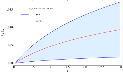
Figure 1: The ratios of $\tilde{c}$ to its present value, $\tilde{c}_{0}$ for different values of $\Omega_{m0}$ as a function of the redshift when $\omega_{0}=-1$. a) $\tilde{c}/\tilde{c}_{0}$ for $\Omega_{m0}=0.29$. The dashed line is the best fit value of it and solid lines are $1$-$\sigma$ error lines. b) $\tilde{c}(z)/\tilde{c}_{0}$ for $\Omega_{m0}=0.30$. The dashed line and solid lines correspond to the best fit value of and 1-$\sigma$ errors, respectively.

III.1.3 $\omega_{0}=-1$ with fixing $h$

We fix the value of $h$ and conduct a maximum likelihood analysis. In these models, both the value of $\Omega_{\text{m}0}(=0.299\pm 0.111)$ and that of $b(=-0.025\pm 0.193)$ do not change even if we vary $h$ from $0.6376$ to $0.74$. As $h$ increases, so does $M_{0}$. The best fit value of $b$ is the same as $-0.025$ for these models. Thus, the speed of light decreases as a function of cosmic time in these models. However, within 1-$\sigma$ error, the values of $b$ are both positive and negative. Thus, one may conclude that there is no variation in the speed of light for these models.

III.1.4 Fixing $h$

We fix the value of $h$ only and do a maximum likelihood analysis. In these models, the best fit values of $M_{0}$, $\omega_{0}$, and $b$ are increased as we vary $h$ from $0.6376$ to $0.74$. However, the best fit value of $\Omega_{\text{m}0}$ decreases as $h$ increases. As $h$ increases, so does $M_{0}$. The best fit values of $b$ are both negative and thus the speed of light decreases as a function of cosmic time in these models. However, within 1-$\sigma$ error, the values of $b$ are both positive and negative and one does not find any variation in the speed of light for these models.

III.1.5 Fixing $\omega_{0}$

We investigate a maximum likelihood analysis for $\omega$CDM models without fixing any cosmological parameters except $\omega_{0}$. We vary the value of $\omega_{0}$ from -0.9 to -1.1. As the value of $\omega_{0}$ decreases, so does $\Omega_{m0}$ but $b$ increases. However, there are no monotonic changes of $M_{0}$ and $h$ in these models. For $\omega_{0}\geq$ -1.0 models, the best fit values of $b$ are negative. Meanwhile, we obtain the positive best fit values of $b$ for $\omega_{0}\leq-1.0$. However, the values of $b$ of all models within 1-$\sigma$ error include both positive and negative values and thus we may conclude there are no variations in the speed of light in these models.

III.2 $\tilde{c}$ for CPL

In this subsection, we repeat the maximum likelihood analysis for the so-called CPL models. We investigate various models for different values of cosmological parameters. The results of the analysis for these models have summarized in table. 2. First we investigate GR (i.e., $b=0$) and extend the analysis for the meVSL models (i.e., $b\neq 0$). Unlike $\omega$CDM models, one is not able to obtain viable $\Omega_{\text{m}0}$-values from this analysis if one does not put any prior in the value of it. Thus, we conduct the maximum likelihood analysis only for the fixed values of $\Omega_{\text{m}0}$.

III.2.1 $b=0$

We investigate CPL models for GR. After we fix $b=0$, we analyze three models, $\omega_{0}=-1$, $\omega_{a}=0$, and without fixing $\omega_{0}$ and $\omega_{a}$. For $\omega_{a}=0$ model, we obtain $0.312\leq\Omega_{\text{m}0}\leq 0.384$, $-1.37\leq\omega_{0}\leq-1.07$, and $0.610\leq h\leq 0.798$ at the $68$ % confidence level. However, if one allows $\omega_{a}$ to vary, then the values of $\Omega_{\text{m}0}$ are too small to be adopted as viable models. When $\omega_{0}=-1.0$, then we obtain $0.94\leq\omega_{a}\leq 1.78$ and $0.109\leq\Omega_{\text{m}0}\leq 0.217$ at $68$ % confidence level. If we allow both $\omega_{0}$ and $\omega_{a}$ to vary, then the allowed regions of cosmological values at $68$ % confidence level are $-0.78\leq\omega_{0}\leq-0.74$, $1.05\leq\omega_{a}\leq 1.55$, and $-0.13\leq\Omega_{\text{m}0}\leq 0.006$.

Now we investigate meVSL models with CPL parameterization of dark energy. It means we probe $b\neq 0$ models.

Table 2: Best fit values and their 1-$\sigma$ errors of cosmological parameters for CPL models. The only green color indicated models are possible to provide the time variation of the speed of light.

Models	$M_{0}$	$\omega_{0}$	$\omega_{a}$	$\Omega_{m0}$	$h$	$b$	$\nu$	$\chi_{\nu}^{2}$
$b=0$	$-19.3617\pm 0.2914$	$-1$	$1.36\pm 0.42$	$0.163\pm 0.054$	$0.704\pm 0.094$	$0$	$1044$	$0.987$
	$-19.3582\pm 0.2915$	$-1.22\pm 0.15$	$0$	$0.348\pm 0.036$	$0.704\pm 0.094$	$0$	$1044$	$0.988$
	$-19.3325\pm 0.0908$	$-0.76\pm 0.02$	$1.30\pm 0.25$	$-0.062\pm 0.068$	$0.712\pm 0.030$	$0$	$1043$	$0.988$
$b\neq 0$	$-19.2231\pm 0.1985$	$-1$	$1.44\pm 0.08$	$-0.102\pm 0.065$	$0.748\pm 0.068$	$0.464\pm 0.156$	$1043$	$0.988$
	$-19.5513\pm 0.1284$	$-1.22\pm 0.04$	$0$	$0.335\pm 0.088$	$0.644\pm 0.038$	$0.022\pm 0.176$	$1043$	$0.989$
$\omega_{0}=-0.95$	$-19.4115\pm 0.2313$		$1.85\pm 0.22$	$0.28$	$0.688\pm 0.073$	$\pagecolor{green}-0.273\pm 0.014$	$1044$	$0.987$
	$-19.4065\pm 0.2324$		$1.90\pm 0.23$	$0.29$	$0.690\pm 0.074$	$-0.291\pm 0.014$	$1044$	$0.987$
	$-19.4110\pm 0.2328$	$-0.95$	$1.95\pm 0.23$	$0.30$	$0.689\pm 0.074$	$-0.309\pm 0.014$	$1044$	$0.987$
	$-19.4114\pm 0.2335$		$2.01\pm 0.24$	$0.31$	$0.689\pm 0.074$	$-0.326\pm 0.014$	$1044$	$0.987$
	$-19.4119\pm 0.2342$		$2.07\pm 0.24$	$0.32$	$0.688\pm 0.074$	$-0.344\pm 0.014$	$1044$	$0.987$
$\omega_{0}=-1.0$	$-19.4108\pm 0.2322$		$1.73\pm 0.23$	$0.28$	$0.689\pm 0.074$	$\pagecolor{green}-0.215\pm 0.015$	$1044$	$0.988$
	$-19.3848\pm 0.2349$		$1.79\pm 0.24$	$0.29$	$0.697\pm 0.075$	$-0.235\pm 0.015$	$1044$	$0.988$
	$-19.4036\pm 0.2344$	$-1.0$	$1.85\pm 0.24$	$0.30$	$0.691\pm 0.075$	$-0.255\pm 0.015$	$1044$	$0.988$
	$-19.4100\pm 0.2346$		$1.91\pm 0.24$	$0.31$	$0.689\pm 0.074$	$-0.274\pm 0.015$	$1044$	$0.988$
	$-19.4107\pm 0.2353$		$1.97\pm 0.25$	$0.32$	$0.689\pm 0.075$	$-0.293\pm 0.015$	$1044$	$0.988$
$\omega_{0}=-1.05$	$-19.4038\pm 0.2339$		$1.57\pm 0.24$	$0.28$	$0.691\pm 0.074$	$\pagecolor{green}-0.154\pm 0.015$	$1044$	$0.988$
	$-19.4076\pm 0.2344$		$1.62\pm 0.25$	$0.29$	$0.689\pm 0.074$	$-0.175\pm 0.015$	$1044$	$0.988$
	$-19.4079\pm 0.2351$	$-1.05$	$1.68\pm 0.25$	$0.30$	$0.689\pm 0.075$	$-0.195\pm 0.015$	$1044$	$0.988$
	$-19.4096\pm 0.2356$		$1.73\pm 0.25$	$0.31$	$0.689\pm 0.075$	$-0.213\pm 0.015$	$1044$	$0.988$
	$-19.4082\pm 0.2367$		$1.84\pm 0.26$	$0.32$	$0.690\pm 0.075$	$-0.240\pm 0.015$	$1044$	$0.988$
fixed $\Omega_{m0}$	$-19.3499\pm 0.1176$	$-1.18\pm 0.04$	$0.72\pm 0.23$	$0.28$	$0.707\pm 0.038$	$\pagecolor{cyan}0.038\pm 0.015$	$1043$	$0.988$
	$-19.3465\pm 0.1199$	$-1.18\pm 0.04$	$0.76\pm 0.25$	$0.30$	$0.708\pm 0.039$	$0.001\pm 0.015$	$1043$	$0.989$
	$-19.3478\pm 0.1225$	$-1.20\pm 0.04$	$0.71\pm 0.26$	$0.32$	$0.708\pm 0.040$	$-0.024\pm 0.015$	$1043$	$0.989$
fixed $h$	$-19.4544\pm 0.0072$	$-0.99\pm 0.02$	$1.31\pm 0.11$	$0.033\pm 0.061$	$0.6736$	$0.207\pm 0.120$	$1043$	$0.988$
	$-19.2475\pm 0.0078$	$-0.99\pm 0.01$	$1.45\pm 0.07$	$-0.112\pm 0.036$	$0.74$	$0.460\pm 0.094$	$1043$	$0.988$
No fixing	$-19.3500\pm 0.0857$	$-0.76\pm 0.02$	$1.30\pm 0.10$	$-0.054\pm 0.086$	$0.706\pm 0.028$	$-0.023\pm 0.108$	$1042$	$0.989$

III.2.2 $\omega_{0}=-0.95$ with fixing $\Omega_{\text{m}0}$

We do a maximum likelihood analysis for $\omega_{0}=-0.95$ models by varying values of $\Omega_{\text{m}0}$ from $0.28$ to $0.32$. For these models, the best fit values of $h$ are all approximately the same as $0.69$ with $0.07$ of 1-$\sigma$ error. As $\Omega_{\text{m}0}$ increases, so does the best fit value of $\omega_{a}$. The best fit values of $b$ decrease for the increasing values of $\Omega_{\text{m}0}$. All $b$-values are negative at a 68 % confidence level for all given values of $\Omega_{\text{m}0}$. They vary from $-0.344\leq b\leq-0.273$ for given values of $\Omega_{\text{m}0}$. Thus, the speed of light is a monotonically decreasing function of a cosmic time and the speed of light decreases faster as the value of $\Omega_{\text{m}0}$ gets larger. At $z=3$, $\tilde{c}$ can be larger than $tc_{0}$ about $10(13)$ % when $\Omega_{\text{m}0}=0.28(0.32)$. The 1-$\sigma$ ranges of $\dot{\tilde{c}}_{0}/\tilde{c}_{0}$ ($10^{-12}\,\text{yr}^{-1}$) are ($-5.05\,,-4.55$)  , (-5.38  , -4.88)  , (-5.69  , -5.20)  , (-5.99  , -5.50)  , and (-6.31  , -5.82), respectively.

III.2.3 $\omega_{0}=-1.0$ with fixing $\Omega_{\text{m}0}$

We repeat the analysis for $\omega_{0}=-1.0$ models. For these models, the best fit values of $h$ range from $0.689$ to $0.697$ for the given values of $\Omega_{\text{m}0}$. The best fit values of $\omega_{a}$ and $b$ are ranged as $1.73\leq\omega_{a}\leq 1.97$ and $-0.293\leq b\leq-0.215$, respectively. The best fit values of $b$ decrease for the increasing values of $\Omega_{\text{m}0}$. For these models, all $b$-values are also negative at a 68 % confidence level for all given values of $\Omega_{\text{m}0}$. Thus, the speed of light is also a monotonically decreasing function of a cosmic time in these models. The decreasing rate of the speed of light for the same value of $\Omega_{\text{m}0}$ is smaller for this model compared to that of $\omega_{0}=-0.95$ model. $\tilde{c}$ at $z=3$ is larger than $tc_{0}$ about $8(10)$ % when $\Omega_{\text{m}0}=0.28(0.32)$. The 1-$\sigma$ ranges of $\dot{\tilde{c}}_{0}/\tilde{c}_{0}$ ($10^{-12}\,\text{yr}^{-1}$) are ($-4.05\,,-3.52$)  , (-4.45  , -3.92)  , (-4.77  , -4.24)  , (-5.09  , -4.56)  , and (-5.42  , -4.89), respectively.

III.2.4 $\omega_{0}=-1.05$ with fixing $\Omega_{\text{m}0}$

Maximum likelihood analysis for $\omega_{0}=-1.05$ models is conducted in this subsection. For these models, the best fit values of $h$ are roughly the same as $0.69$ for all given values of $\Omega_{\text{m}0}$. The best fit values of $\omega_{a}$ and $b$ are ranged as $1.57\leq\omega_{a}\leq 1.84$ and $-0.240\leq b\leq-0.154$, respectively. The best fit values of $b$ also decrease for the increasing values of $\Omega_{\text{m}0}$ in these models. $b$-values are $-0.169\leq b\leq-0.139$ for $\Omega_{\text{m}0}=0.28$ and $-0.255\leq b\leq-0.225$ for $\Omega_{\text{m}0}=0.32$ within 1-$\sigma$ error. Thus, the speed of light is also a monotonically decreasing function of a cosmic time in these models. At $z=3$, $\tilde{c}$ can be larger than $tc_{0}$ about $6(9)$ % when $\Omega_{\text{m}0}=0.28(0.32)$. The decreasing rate of the speed of light for the same value of $\Omega_{\text{m}0}$ is smaller for this model compared to those of $\omega_{0}=-0.95$ and $-1.0$ models. The 1-$\sigma$ ranges of $\dot{\tilde{c}}_{0}/\tilde{c}_{0}$ ($10^{-12}\,\text{yr}^{-1}$) are ($-2.98\,,-2.45$)  , (-3.44  , -2.82)  , (-3.70  , -3.17)  , (-4.01  , -3.49)  , and (-4.50  , -3.97), respectively.

III.2.5 CPL with fixing $\Omega_{\text{m}0}$

We analyze the Pantheon data without constraining values of $\omega_{0}$ and $\omega_{a}$ for $0.28\leq\Omega_{\text{m}0}\leq 0.32$. For these models, the best fit values of $h$ are roughly the same as $0.71$ for all given values of $\Omega_{\text{m}0}$. Best fit values of both $\omega_{0}$ and $\omega_{a}$ are ($-1.18\,,0.72$), ($-1.18\,,0.76$), and ($-1.20\,,0.71$) for $\Omega_{\text{m}0}=0.28,0.30$, and 0.32, respectively. Interesting model is $\Omega_{\text{m}0}=0.30$. In this model, the best fit value of $b$ is almost zero. It varies from $-0.015$ to $0.015$ at a $68$ % confidence level. Thus, there is no time variation of the speed of light in this model. However, the 1-$\sigma$ values of $b$ are ranged as $0.023\leq b\leq 0.053$ for $\Omega_{\text{m}0}=0.28$ and $-0.039\leq b\leq-0.009$ for $\Omega_{\text{m}0}=0.32$. Thus, the speed of light is monotonically decreasing (increasing) function of the cosmic time for $\Omega_{\text{m}0}=0.28(0.32)$ at 68 % confidence level. This is shown in figure. 2. In the left panel of Fig. 2, the cosmological evolutions of $\tilde{c}/\tilde{c}_{0}$ as a function of $z$ for $\Omega_{\text{m}0}=0.28$ model are depicted. The dashed line corresponds to the best fit value of $b$ and the solid lines indicate those of 1-$\sigma$ errors. $\tilde{c}/\tilde{c}_{0}$ decreases monotonically when the redshift increases because all of $b$ are positive. $\tilde{c}$ decreases about $0.8(1.8)$ % within 1-$\sigma$ error at $z=3$. $\dot{\tilde{c}}_{0}/\tilde{c}_{0}\,(10^{-13}\,\text{yr}^{-1})$ ranges (4.15  , 9.57) at a 68 % confidence level. Meanwhile, the right panel of Fig. 2 depicts the model, $\Omega_{\text{m}0}=0.32$. Values of both the best fit and 1-$\sigma$ error are negative and thus $\tilde{c}/\tilde{c}_{0}$ are monotonically increasing functions of the redshift, $z$. At $z=3$, $\tilde{c}$ increases about $0.3(1.4)$ % at 68 % confidence level. The 1-$\sigma$ range of $\dot{\tilde{c}}_{0}/\tilde{c}_{0}$ ($10^{-13}\,\text{yr}^{-1}$) is ($-7.05\,,-1.63$).

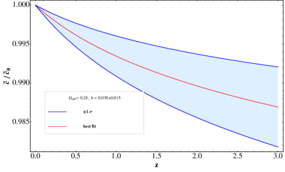
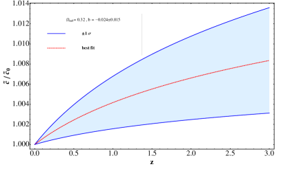
Figure 2: The ratios of $\tilde{c}(z)$ to its present value, $\tilde{c}_{0}$, for different values of $\Omega_{m0}$ as a function of the redshift. a) $\tilde{c}/\tilde{c}_{0}$ for $\Omega_{m0}=0.28$. The dashed line is the best fit value of it and solid lines are $1$-$\sigma$ error lines. b) $\tilde{c}/\tilde{c}_{0}$ for $\Omega_{m0}=0.32$. The dashed line and solid lines correspond to the best fit value of and 1-$\sigma$ errors, respectively.

III.2.6 CPL with (without) fixing $h$

The analysis is done for fixed values of $h$ without constraining any other parameters. Best fit values and 1-$\sigma$ error for $\omega_{0}$ and $\omega_{a}$ are given by $-0.99\pm 0.02(-0.99\pm 0.01)$ and $1.31\pm 0.11(1.45\pm 0.07)$ for $h=0.6736(0.74)$. In these models $b$ are positive. However, the obtained values of $\Omega_{\text{m}0}$ are $-0.028\leq\Omega_{\text{m}0}\leq 0.094\,(-0.148\leq\Omega_{\text{m}0}\leq-0.076)$ for $h=0.6736\,(0.74)$ and this is not viable. If we do not constrain $\Omega_{\text{m}0}$, then the obtained value of matter density contrast is $-0.14\leq\Omega_{\text{m}0}\leq 0.032$. This is not viable either.

III.3 $\dot{\tilde{c}}$ and $\dot{\tilde{G}}$

From previous subsections III.1 and III.2, we investigate viable meVSL models for different dark energy models and obtain constraints on parameters of both cosmological and model parameters. We estimate the time variation of the speed of light from these constraints. In the meVSL model, not only the speed of light but also the gravitational constant evolve cosmologically as $\tilde{G}=\tilde{G}_{0}(1+z)^{-b}$. Thus, we can estimate the bounds on the present value of the relative temporal variation of the gravitational constant, $\dot{\tilde{G}}_{0}/\tilde{G}_{0}$ by using obtained constraints on $b$-values. In order to compare these results with other observations, we show current bounds on $\dot{\tilde{G}}_{0}/\tilde{G}_{0}$ from various observations in table. 3. Among these, analysis of lunar laser ranging (LLR) data provides the lowest bounds on $\dot{\tilde{G}}_{0}/\tilde{G}_{0}$. The orbital period rate of pulsars gives the largest bounds as $2.3\times 10^{-11}\,\text{yr}^{-1}$. Roughly, one can claim that $\dot{\tilde{G}}_{0}/\tilde{G}_{0}$ is about the order of $10^{-12}\,\text{yr}^{-1}$.

Table 3: Current observational 1-$\sigma$ bounds on a present value of the relative temporal variation of the gravitational constant, $\dot{\tilde{G}}_{0}/\tilde{G}_{0}$. WD means white dwarf, BBN denotes big bang nucleosynthesis, LLR represents lunar laser ranging, GWs means gravitational waves.

obs	$\dot{\tilde{G}}_{0}/\tilde{G}_{0}\,(10^{-12}\,\text{yr}^{-1})$	Ref
pulsars	23	Verbiest:2008gy
WD cooling	-1.8	GarciaBerro:2011wc
pulsation	-130	Corsico:2013ida
BBN	$-0.3\sim 0.4$	Bambi:2005fi
	$-3.6\sim 4.5$	Alvey:2019ctk
LLR	$-0.5\sim 0.9$	Hofmann:2010
	$-0.005\sim 0.147$	Hofmann:2018
SNe Ia	$-30\sim 73$	Mould:2014iga
	$3$	Zhao:2018gwk
GWs LIGO	$70$	Lagos:2019kds
LISA	$0.7$	Belgacem:2019pkk

The results of the time variations of both the speed of light and the gravitational constant of meVSL models for various dark energy models are shown in table 4. We denote $\Delta\tilde{c}(z=3)$ as the percentage difference between the value of the speed of light at $z=3$ and its present value, $\Delta\tilde{c}(z=3)\equiv\left(\tilde{c}(z=3)-\tilde{c}_{0}\right)/\tilde{c}_{0}\times 100\,(\%)$ within 1-$\sigma$ error. Also, $\Delta\tilde{G}(z=3)$ represents the percentage difference between the value of the gravitational constant at $z=3$ and that at $z=0$. The ratio of the time variation of the speed of light to the speed of light at the present epoch is denoted by $\dot{\tilde{c}}_{0}/\tilde{c}_{0}$. $\dot{\tilde{G}}_{0}/\tilde{G}_{0}$ indicates the present value of the ratio of the time variation of the gravitational constant to itself. The best fit value of $b$ and its values within 68 % confidence level are positive only for CPL dark energy model when $\Omega_{\text{m}0}=0.28$. Thus, $\dot{\tilde{c}}_{0}/\tilde{c}_{0}$ and $\dot{\tilde{G}}_{0}/\tilde{G}_{0}$ are positive for this model. All other viable models analyzed by using the Pantheon data give the negative values of $b$ and thus both $\dot{\tilde{c}}_{0}/\tilde{c}_{0}$ and $\dot{\tilde{G}}_{0}/\tilde{G}_{0}$ are negative in these models. $\dot{\tilde{c}}_{0}/\tilde{c}_{0}$s are the order of $10^{-13}\,\text{yr}^{-1}$ and $\dot{\tilde{G}}_{0}/\tilde{G}_{0}$s are the order of $10^{-12}\,\text{yr}^{-1}$ for $\omega$CDM models and CPL models with varying both $\omega_{0}$ and $\omega_{a}$ as shown in table. 4. However, $\dot{\tilde{c}}_{0}/\tilde{c}_{0}$s are order of $10^{-12}\,\text{yr}^{-1}$ and $\dot{\tilde{G}}_{0}/\tilde{G}_{0}$s are the order of $10^{-11}\,\text{yr}^{-1}$ for CPL models with the fixed $\omega_{0}$.

Table 4: Time variations of the speed of light and that of the gravitational constant at a 68 % confidence level for viable models.

$\omega_{0}$	$\omega_{a}$	$\Omega_{\text{m}0}$	$\Delta\tilde{c}(z=3)\,(\%)$	$\dot{\tilde{c}}_{0}/\tilde{c}_{0}\,(10^{-13}\,\text{yr}^{-1})$	$\Delta\tilde{G}(z=3)\,(\%)$	$\dot{\tilde{G}}_{0}/\tilde{G}_{0}\,(10^{-12}\,\text{yr}^{-1})$
-1	0	$0.30$	$0.2\sim 1.7$	$-8.76\sim-0.89$	$0.7\sim 7.0$	$-3.51\sim-0.36$
		$0.31$	$0.8\sim 2.3$	$-1.18\sim-0.39$	$3.1\sim 9.6$	$-4.72\sim-1.57$
		$0.32$	$1.4\sim 2.9$	$-1.48\sim-0.70$	$5.6\sim 12.2$	$-5.94\sim-2.79$
-0.95	$1.85\pm 0.22$	$0.28$	$9.4\sim 10.5$	$-51.3\sim-46.3$	$43.2\sim 48.9$	$-20.5\sim-18.5$
	$1.95\pm 0.23$	$0.30$	$10.8\sim 11.8$	$-57.8\sim-52.8$	$50.5\sim 56.5$	$-23.1\sim-21.1$
	$2.07\pm 0.24$	$0.32$	$12.1\sim 13.2$	$-64.0\sim-59.0$	$58.0\sim 64.3$	$-25.6\sim-23.6$
-1.0	$1.73\pm 0.23$	$0.28$	$7.2\sim 8.3$	$-41.1\sim-35.8$	$32.0\sim 37.6$	$-16.5\sim-14.3$
	$1.85\pm 0.24$	$0.30$	$8.7\sim 9.8$	$-48.3\sim-42.9$	$39.5\sim 45.4$	$-19.3\sim-17.2$
	$1.97\pm 0.25$	$0.32$	$10.1\sim 11.3$	$-55.1\sim-49.7$	$47.0\sim 53.2$	$-22.0\sim-19.9$
-1.05	$1.57\pm 0.24$	$0.28$	$4.9\sim 6.0$	$-30.2\sim-24.9$	$21.3\sim 26.4$	$-12.1\sim-9.9$
	$1.68\pm 0.25$	$0.30$	$6.4\sim 7.5$	$-37.6\sim-32.2$	$28.3\sim 33.8$	$-15.0\sim-12.9$
	$1.84\pm 0.26$	$0.32$	$8.1\sim 9.2$	$-45.6\sim-40.2$	$36.6\sim 42.4$	$-18.2\sim-16.1$
$-1.18\pm 0.04$	$0.72\pm 0.23$	$0.28$	$0.8\sim 1.8$	$4.11\sim 9..48$	$3.1\sim 7.1$	$1.65\sim 3.79$
$-1.20\pm 0.04$	$0.71\pm 0.26$	$0.32$	$0.3\sim 1.4$	$-6.98\sim-1.61$	$1.3\sim 5.6$	$-2.79\sim-0.64$

IV Conclusions

The Pantheon data can constrain cosmological and model parameters to the statistically about 10 %. Thus, we adopt this data and use a maximum likelihood analysis to constrain dark energy models based on the meVSL model. From this, we obtain several viable $\omega$CDM and CPL dark energy models and get constrain on the value of $b$ which determines the cosmological evolutions of physical constants. We obtain constraints $-64.0\leq\dot{\tilde{c}}_{0}/\tilde{c}_{0}\,(10^{-13}\,\text{yr}^{-1})\leq-0.39$ and $-25.6\leq\dot{\tilde{G}}_{0}/\tilde{G}_{0}\,(10^{-12}\,\text{yr}^{-1})\leq-0.36$ for most viable models. Thus, we conclude that current Pantheon data show that both the speed of light and the gravitational constant are larger in the past and monotonically increase as a function of the redshift, $z$.

We may further constrain cosmological and model parameters if we add other cosmological observations, like CMB, BAO, and etc. However, we need to reanalyze those data based on the theoretical values of the meVSL model. This is out of the scope of this manuscript and we postpone this for future work.

References

- (1) S. Lee, [arXiv:2011.09274 [astro-ph.CO]].
- (2) D. M. Scolnic, D. O. Jones, A. Rest, Y. C. Pan, R. Chornock, R. J. Foley, M. E. Huber, R. Kessler, G. Narayan and A. G. Riess, et al. Astrophys. J. 859, no.2, 101 (2018) doi:10.3847/1538-4357/aab9bb [arXiv:1710.00845 [astro-ph.CO]].
- (3) M. Chevallier and D. Polarski, Int. J. Mod. Phys. D 10, 213-224 (2001) doi:10.1142/S0218271801000822 [arXiv:gr-qc/0009008 [gr-qc]].
- (4) E. V. Linder, Phys. Rev. Lett. 90, 091301 (2003) doi:10.1103/PhysRevLett.90.091301 [arXiv:astro-ph/0208512 [astro-ph]].
- (5) J. C. B. Sanchez and L. Perivolaropoulos, Phys. Rev. D 81, 103505 (2010) doi:10.1103/PhysRevD.81.103505 [arXiv:1002.2042 [astro-ph.CO]].
- (6) J. Racker, P. Sisterna and H. Vucetich, Phys. Rev. D 80, 083526 (2009) doi:10.1103/PhysRevD.80.083526 [arXiv:0711.0797 [astro-ph]].
- (7) M. McElhinny, S. Taylor, and D. Stevenson, Nature 271, 316 (1978) https://doi.org/10.1038/271316a0.
- (8) J. Magueijo, Phys. Rev. D 62, 103521 (2000) doi:10.1103/PhysRevD.62.103521 [arXiv:gr-qc/0007036 [gr-qc]].
- (9) J. P. W. Verbiest, M. Bailes, W. van Straten, G. B. Hobbs, R. T. Edwards, R. N. Manchester, N. D. R. Bhat, J. M. Sarkissian, B. A. Jacoby and S. R. Kulkarni, Astrophys. J. 679, 675-680 (2008) doi:10.1086/529576 [arXiv:0801.2589 [astro-ph]].
- (10) E. Garcia-Berro, P. Loren-Aguilar, S. Torres, L. G. Althaus and J. Isern, JCAP 05, 021 (2011) doi:10.1088/1475-7516/2011/05/021 [arXiv:1105.1992 [gr-qc]].
- (11) A. H. Córsico, L. G. Althaus, E. García-Berro and A. D. Romero, JCAP 06, 032 (2013) doi:10.1088/1475-7516/2013/06/032 [arXiv:1306.1864 [astro-ph.SR]].
- (12) C. Bambi, M. Giannotti and F. L. Villante, Phys. Rev. D 71, 123524 (2005) doi:10.1103/PhysRevD.71.123524 [arXiv:astro-ph/0503502 [astro-ph]].
- (13) J. Alvey, N. Sabti, M. Escudero and M. Fairbairn, Eur. Phys. J. C 80, no.2, 148 (2020) doi:10.1140/epjc/s10052-020-7727-y [arXiv:1910.10730 [astro-ph.CO]].
- (14) F. Hofmann, J. Müller, and L. Biskupek, Astron. Astrophys 522, L5 (2010) doi:10.1051/0004-6361/201015659.
- (15) F. Hofmann and J. Müller, Class. Quant. Grav 35, 035015 (2018).
- (16) J. Mould and S. Uddin, Publ. Astron. Soc. Austral. 31, 15 (2014) doi:10.1017/pasa.2014.9 [arXiv:1402.1534 [astro-ph.CO]].
- (17) W. Zhao, B. S. Wright and B. Li, JCAP 10, 052 (2018) doi:10.1088/1475-7516/2018/10/052 [arXiv:1804.03066 [astro-ph.CO]].
- (18) M. Lagos, M. Fishbach, P. Landry and D. E. Holz, Phys. Rev. D 99, no.8, 083504 (2019) doi:10.1103/PhysRevD.99.083504 [arXiv:1901.03321 [astro-ph.CO]].
- (19) E. Belgacem et al. [LISA Cosmology Working Group], JCAP 07, 024 (2019) doi:10.1088/1475-7516/2019/07/024 [arXiv:1906.01593 [astro-ph.CO]].