High-Confidence Off-Policy (or Counterfactual) Variance Estimation

Abstract

Many sequential decision-making systems leverage data collected using prior policies to propose a new policy. For critical applications, it is important that high-confidence guarantees on the new policy’s behavior are provided before deployment, to ensure that the policy will behave as desired. Prior works have studied high-confidence off-policy estimation of the expected return, however, high-confidence off-policy estimation of the variance of returns can be equally critical for high-risk applications. In this paper we tackle the previously open problem of estimating and bounding, with high confidence, the variance of returns from off-policy data.

Introduction

Reinforcement learning (RL) has emerged as a promising method for solving sequential decision-making problems (Sutton and Barto 2018). Deploying RL to real-world applications, however, requires additional consideration of reliability, which has been relatively understudied. Specifically, it is often desirable to provide high-confidence guarantees on the behavior of a given policy, before deployment, to ensure that the policy will behave as desired.

Prior works in RL have studied the problem of providing high-confidence guarantees on the expected return of an evaluation policy, $\pi$, using only data collected from a currently deployed policy called the behavior policy, $\beta$ (Thomas, Theocharous, and Ghavamzadeh 2015; Hanna, Stone, and Niekum 2017; Kuzborskij et al. 2020). Analogously, researchers have also studied the problem of counter-factually estimating and bounding the average treatment effect, with high confidence, using data from past treatments (Bottou et al. 2013). While these methods present important contributions towards developing practical algorithms, real-world problems may require additional consideration of the variance of returns (effect) under any new policy (treatment) before it can be deployed responsibly.

For applications that have high stakes in the terms of financial cost or public well-being, only providing guarantees on the mean outcome might not be sufficient. Analysis of variance (ANOVA) has therefore become a de-facto standard for many industrial and medical applications (Tabachnick and Fidell 2007). Similarly, analysis of variance can inform numerous real-world applications of RL. For example, (a) analysing the variance of outcomes in a robotics application (Kuindersma, Grupen, and Barto 2013), (b) ensuring that the variance of outcomes for a medical treatment is not high, (c) characterizing the variance of customer experiences for a recommendation system (Teevan et al. 2009), or (d) limiting the variability of the performance of an autonomous driving system (Montgomery 2007).

More generally, variance estimation can be used to account for risk in decision-making by designing objectives that maximize the mean of returns but minimize the variance of returns (Sato, Kimura, and Kobayashi 2001; Di Castro, Tamar, and Mannor 2012; La and Ghavamzadeh 2013). Variance estimates have also been shown to be useful for automatically adapting hyper-parameters, like the exploration rate (Sakaguchi and Takano 2004) or $\lambda$ for eligibility-traces (White and White 2016), and might also inform other methods that depend on the entire distribution of returns (Bellemare, Dabney, and Munos 2017; Dabney et al. 2017).

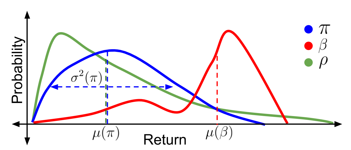
Figure 1: Illustrative example of the distributions of returns from a behavior policy $\beta$, and evaluation policy $\pi$, along with the importance weighted returns $\rho$, discussed later. Given trajectories from the behavior policy $\beta$, we aim to estimate and bound the variance, $\sigma^{2}(\pi)$, of returns under an evaluation policy $\pi$, with high confidence. Note that the distribution of importance-weighted returns $\rho$ has the mean value $\mu(\pi)$, but might have variance not equal to $\sigma^{2}(\pi)$.

Despite the wide applicability of variance analysis, estimating and bounding the variance of returns with high confidence, using only off-policy data, has remained an understudied problem. In this paper, we first formalize the problem statement; an illustration of which is provided in Figure 1. We show that the typical use of importance sampling (IS) in RL only corrects for the mean, and so it does not directly provide unbiased off-policy estimates of variance. We then present an off-policy estimator of the variance of returns that uses IS twice, together with a simple double-sampling technique. To reduce the variance of the estimator, we extend the per-decision IS technique (Precup 2000) to off-policy variance estimation. Building upon this estimator, we provide confidence intervals for the variance using (a) concentration inequalities, and (b) statistical bootstrapping.

Advantages: The proposed variance estimator has several advantages: (a) it is a model-free estimator and can thus be used irrespective of the environment complexity, (b) it requires only off-policy data and can therefore be used before actual policy deployment, (c) it is unbiased and consistent. For high-confidence guarantees, (d) we provide both upper and lower confidence intervals for the variance that have guaranteed coverage (that is, they hold with any desired confidence level and without requiring false assumptions), and (e) we also provide bootstrap confidence intervals, which are approximate but often more practical.

Limitations: The proposed off-policy estimator of the variance relies upon IS and thus inherits its limitations. Namely, (a) it requires knowledge of the action probabilities from the behavior policy $\beta$, (b) it requires that the support of the trajectories under the evaluation policy $\pi$ is a subset of the support under the behavior policy $\beta$, and (c) the variance of the estimator scales exponentially with the length of the trajectory (Guo, Thomas, and Brunskill 2017; Liu et al. 2018).

Background and Problem Statement

A Markov decision process (MDP) is a tuple $(\mathcal{S},\mathcal{A},\mathcal{P},\mathcal{R},\gamma,d_{0})$, where $\mathcal{S}$ is the set of states, $\mathcal{A}$ is the set of actions, $\mathcal{P}$ is the transition function, $\mathcal{R}$ is the reward function, $\gamma\in[0,1)$ is the discount factor, and $d_{0}$ is the starting state distribution. A policy $\pi$ is a distribution over the actions conditioned on the state, i.e., $\pi(a|s)$ represents the probability of taking action $a$ in state $s$. We assume that the MDP has finite horizon $T$, after which any action leads to an absorbing state $S_{(\infty)}$. In general, we will use subscripts with parentheses for the timestep and subscript without parentheses to indicate the episode number. Let $R_{i(j)}\in[R_{\texttt{min}},R_{\texttt{max}}]$ represent the reward observed at timestep $j$ of the episode $i$. Let the random variable $G_{i}\coloneqq\sum_{j=0}^{T}\gamma^{j}R_{i(j)}$ be the return for episode $i$. Let $c\coloneqq(1-\gamma^{T})/(1-\gamma)$ so that the minimum and the maximum returns possible are $G_{\texttt{min}}\coloneqq cR_{\texttt{min}}$ and $G_{\texttt{max}}\coloneqq cR_{\texttt{max}}$, respectively. Let $\mu(\pi)\coloneqq\mathbb{E}_{\pi}[G]$ be the expected return, and $\sigma^{2}(\pi)\coloneqq\mathbb{V}_{\pi}[G]$ be the variance of returns, where the subscript $\pi$ denotes that the trajectories are generated using policy $\pi$.

Let $\mathcal{H}^{\pi}_{(i):(j)}$ be the set of all possible trajectories for a policy $\pi$, from timestep $i$ to timestep $j$. Let $H$ denote a complete trajectory: $(S_{(0)},A_{(0)},\Pr(A_{(0)}|S_{(0)}),R_{(0)},S_{(1)},...,S_{(\infty)})$, where $T$ is the horizon length, and $S_{(0)}$ is sampled from $d_{0}$. Let $\mathcal{D}$ be a set of $n$ trajectories $\{H_{i}\}_{i=1}^{n}$ generated using behavior policies $\{\beta_{i}\}_{i=1}^{n}$, respectively. Let $\rho_{i}(0,T)\coloneqq\prod_{j=0}^{T}\frac{\pi(A_{i(j)}|S_{i(j)})}{\beta_{i}(A_{i(j)}|S_{i(j)})}$ denote the product of importance ratios from timestep $0$ to $T$. For brevity, when the range of timesteps is not necessary, we write $\rho_{i}\coloneqq\rho_{i}(0,T)$. Similarly, when referring to $\rho_{i}$ for an arbitrary $i\in\{1,\dotsc,n\}$, we often write $\rho$. With this notation, we now formalize the off-policy variance estimation (OVE) and the high-confidence off-policy variance estimation (HCOVE) problems.

OVE Problem:

Given a set of trajectories $\mathcal{D}$ and an evaluation policy $\pi$, we aim to find an estimator $\hat{\sigma}_{n}^{2}$ that is both an unbiased and consistent estimator of $\sigma^{2}(\pi)$, i.e.,

$$\mathbb{E}[\hat{\sigma}_{n}^{2}] =\sigma^{2}(\pi), \hat{\sigma}_{n}^{2} \overset{\text{a.s.}}{\longrightarrow}\sigma^{2}(\pi).$$ (1)

HCOVE Problem:

Given a set of trajectories $\mathcal{D}$, an evaluation policy $\pi$, and a confidence level $1-\delta$, we aim to find a confidence interval $\mathcal{C}\coloneqq[v^{\texttt{lb}},v^{\texttt{ub}}]$, such that

$$\Pr\left(\sigma^{2}(\pi)\in\mathcal{C}\right)\geq 1-\delta.$$ (2)

Remark 1.

It is worth emphasizing that the OVE problem is about estimating the variance of returns, and not the variance of the estimator of the mean of returns.

These problems would not be possible to solve if the trajectories in $\mathcal{D}$ are not informative about the trajectories that are possible under $\pi$. For example, if $\mathcal{D}$ has no trajectory that could be observed if policy $\pi$ were to be executed, then $\mathcal{D}$ provides little or no information about the possible outcomes under $\pi$. To avoid this case, we make the following common assumption (Precup 2000), which is satisfied if $(\beta_{i}(a|s)=0)\implies(\pi(a|s)=0)$ for all $s\in\mathcal{S},a\in\mathcal{A},$ and $i\in\{1,\dotsc,n\}$.

Assumption 1.

The set $\mathcal{D}$ contains independent trajectories generated using behavior policies $\{\beta_{i}\}_{i=1}^{n}$, such that

$$\forall i,\,\,\mathcal{H}^{\pi}_{(0):(T)}\subseteq\mathcal{H}^{\beta_{i}}_{(0):(T)}.$$

ass:supp

The methods that we derive, and IS methods in general, do not require complete knowledge of $\{\beta_{i}\}_{i=1}^{n}$ (which might be parameterized using deep neural networks and might be hard to store). Only the probabilities, $\beta_{i}(a|s)$, for states $s$ and actions $a$ present in $\mathcal{D}$ are required. For simplicity, we restrict our notation to a single behavior policy $\beta$, such that $\forall i,\,\,\beta_{i}=\beta$.

Naïve Methods

In the on-policy setting, computing an estimate of $\mu(\pi)$ or $\sigma^{2}(\pi)$ is trivial—sample $n$ trajectories using $\pi$ and compute the sample mean or variance of the observed returns, $\{G_{i}\}_{i=1}^{n}$. In the off-policy setting, under ass:supp, the sample mean $\hat{\mu}\coloneqq\frac{1}{n}\sum_{i=1}^{n}\rho_{i}G_{i}$ of the importance weighted returns $\{\rho_{i}G_{i}\}_{i=1}^{n}$, is an unbiased estimator of $\mu(\pi)$ (Precup 2000), i.e., $\mathbb{E}_{\beta}[\hat{\mu}]=\mu(\pi)$. Similarly, one natural way to estimate $\sigma^{2}(\pi)$ in the off-policy setting might be to compute the sample variance (with Bessel’s correction) of the importance sampled returns $\{\rho_{i}G_{i}\}_{i=1}^{n}$,

$$\hat{\sigma}_{n}^{2!!}\coloneqq\frac{1}{n-1}\sum_{i=1}^{n}\left(\rho_{i}G_{i}-\frac{1}{n}\sum_{j=1}^{n}\rho_{j}G_{j}\right)^{2}.$$ (3)

Unfortunately, $\hat{\sigma}_{n}^{2!!}$ is neither an unbiased nor consistent estimator of $\sigma^{2}(\pi)$, in general, as shown in the following properties. These properties also reveal that $\rho_{i}G_{i}$ only corrects the distribution for the mean and not for the variance, as depicted in Figure 1. Also, note that all proofs are deferred to the appendix.

Property 1.

Under ass:supp, $\hat{\sigma}_{n}^{2!!}$ may be a biased estimator of $\sigma^{2}(\pi)$. That is, it is possible that $\mathbb{E}_{\beta}[\hat{\sigma}_{n}^{2!!}]\neq\sigma^{2}(\pi)$. prop:naive1biased

Property 2.

Under ass:supp, $\hat{\sigma}_{n}^{2!!}$ may not be a consistent estimator of $\sigma^{2}(\pi)$. That is, it is not always the case that $\hat{\sigma}_{n}^{2!!}\overset{\text{a.s.}}{\longrightarrow}\sigma^{2}(\pi)$. prop:naive1inconsistent

Since the on-policy variance is $\mathbb{E}_{\pi}[(G-\mathbb{E}_{\pi}[G])^{2}]$, a natural alternative might be to construct an estimator that corrects the off-policy distribution for both the mean and the variance. That is, using the equivalence

$$\mathbb{V}_{\pi}(G)=\mathbb{E}_{\pi}[(G-\mathbb{E}_{\pi}[G])^{2}]=\mathbb{E}_{\beta}[\rho(G-\mathbb{E}_{\beta}[\rho G])^{2}],$$ (4)

an alternative might be to use a plug-in estimator for $\mathbb{E}_{\beta}[\rho(G-\mathbb{E}_{\beta}[\rho G])^{2}]$ (with Bessel’s correction) as,

$$\hat{\sigma}_{n}^{2!}\coloneqq\frac{1}{n-1}\sum_{i=1}^{n}\rho_{i}\left(G_{i}-\frac{1}{n}\sum_{j=1}^{n}\rho_{j}G_{j}\right)^{2}.$$ (5)

While $\hat{\sigma}_{n}^{2!}$ turns out to be a consistent estimator, it is still not an unbiased estimator of $\sigma^{2}(\pi)$. We formalize this in the following properties.

Property 3.

Under ass:supp, $\hat{\sigma}_{n}^{2!}$ may be a biased estimator of $\sigma^{2}(\pi)$. That is, it is possible that $\mathbb{E}_{\beta}[\hat{\sigma}_{n}^{2!}]\neq\sigma^{2}(\pi)$. prop:naive2biased

Property 4.

Under ass:supp, $\hat{\sigma}_{n}^{2!}$ is a consistent estimator of $\sigma^{2}(\pi)$. That is, $\hat{\sigma}_{n}^{2!}\overset{\text{a.s.}}{\longrightarrow}\sigma^{2}(\pi)$. prop:naive2consistent

Before even considering confidence intervals for $\sigma^{2}(\pi)$, the lack of unbiased estimates from these naïve methods leads to a basic question: How can we construct unbiased estimates of $\sigma^{2}(\pi)$? We answer this question in the following section.

Off-Policy Variance Estimation

Before constructing an unbiased estimator for $\sigma^{2}(\pi)$, we first discuss one root cause for the bias of $\hat{\sigma}_{n}^{2!}$ and $\hat{\sigma}_{n}^{2!!}$. Notice that an expansion of (3) and (5) produces self-coupled importance ratio terms. That is, terms consisting of $\rho_{i}^{2}$ and $\rho_{i}^{3}$. While $\rho_{i}$ helps in correcting the distribution, its higher powers, $\rho_{i}^{2}$ and $\rho_{i}^{3}$, do not.

Expansion of (3) and (5) also results in cross-coupled importance ratio terms, $\rho_{i}\rho_{j}$, where $i\neq j$. However, because $\mathbb{E}_{\beta}[\rho_{i}]=1$ for all $i\in\{1,\dotsc,n\}$ and because $\rho_{i}$ and $\rho_{j}$ are independent when $i\neq j$, these terms factor out in expectation. Hence, these terms do not create the troublesome higher powers of importance ratios.

Based on these observations, we create an estimator that does not have any self-coupled importance ratio terms like $\rho_{i}^{2}$, but which may have $\rho_{i}\rho_{j}$ terms, where $i\neq j$. To do so, we consider the alternate formulation of variance,

$$\mathbb{V}_{\pi}(G)=\mathbb{E}_{\pi}[G^{2}]-\mathbb{E}_{\pi}[G]^{2}=\mathbb{E}_{\beta}[\rho G^{2}]-\mathbb{E}_{\beta}[\rho G]^{2}.$$ (6)

In (6), while a plug-in estimator of $\mathbb{E}_{\beta}[\rho G^{2}]$ would be unbiased and free of any self-coupled importance ratio terms, a plug-in estimator for $\mathbb{E}_{\beta}[\rho G]^{2}$ would neither be unbiased nor would it be free of $\rho^{2}_{i}$ terms. To remedy this problem, we explicitly split the set of sampled trajectories into two mutually exclusive sets, $\mathcal{D}_{1}$ and $\mathcal{D}_{2}$, of equal sizes, and re-express $\mathbb{E}_{\beta}[\rho G]^{2}$ as $\mathbb{E}_{\beta}[\rho G]\mathbb{E}_{\beta}[\rho G]$, where the first expectation is estimated using samples from $\mathcal{D}_{1}$ and the second expectation is estimated using samples from $\mathcal{D}_{2}$. Based on this double sampling approach, we propose the following off-policy variance estimator,

$$\hat{\sigma}_{n}^{2}\coloneqq\frac{1}{n}\sum_{i=1}^{n}\rho_{i}G_{i}^{2}-\left(\frac{1}{|\mathcal{D}_{1}|}\sum_{i=1}^{|\mathcal{D}_{1}|}\rho_{i}G_{i}\right)\left(\frac{1}{|\mathcal{D}_{2}|}\sum_{i=1}^{|\mathcal{D}_{2}|}\rho_{i}G_{i}\right).$$ (7)

This simple data-splitting trick suffices to create, $\hat{\sigma}_{n}^{2}$, an off-policy variance estimator that is both unbiased and consistent. We formalize this in the following theorems.

Theorem 1.

Under ass:supp, $\hat{\sigma}_{n}^{2}$ is an unbiased estimator of $\sigma^{2}(\pi)$. That is, $\mathbb{E}_{\beta}[\hat{\sigma}_{n}^{2}]=\sigma^{2}(\pi)$. thm:unbiased

Theorem 2.

Under ass:supp, $\hat{\sigma}_{n}^{2}$ is a consistent estimator of $\sigma^{2}(\pi)$. That is, $\hat{\sigma}_{n}^{2}\overset{\text{a.s.}}{\longrightarrow}\sigma^{2}(\pi)$. thm:consistent

Remark 2.

It is possible that $\hat{\sigma}_{n}^{2}$ results in negative values (see Appendix C for an example). One practical solution to avoid negative values for variance can be to define $\hat{\sigma}_{n}^{2+}\coloneqq\texttt{clip}(\hat{\sigma}_{n}^{2},\texttt{min}=0,\texttt{max}=\infty)$. However, this may make $\hat{\sigma}_{n}^{2+}$ a biased estimator, i.e., $\mathbb{E}_{\beta}[\hat{\sigma}_{n}^{2+}]\neq\sigma^{2}(\pi)$. Notice that this is the expected behavior of IS based estimators. For example, the IS estimates of expected return can be smaller or larger than the smallest and largest possible returns when $\rho>1$. We refer the reader to the works by McHugh and Mielke (1968), Anderson (1965), and Nelder (1954) for other occurences of negative variance and its interpretations.

Variance-Reduced Estimation of Variance

Despite $\hat{\sigma}_{n}^{2}$ being both an unbiased and a consistent estimator of variance, the use of IS can make its variance high. Specifically, the importance ratio $\rho$ may become unstable when its denominator, $\prod_{i=0}^{T}\beta(A_{(i)}|S_{(i)})$, is small.

To mitigate variance, it is common in off-policy mean estimation to use per-decision importance sampling (PDIS), instead of the full-trajectory IS, to reduce variance without incurring any bias (Precup 2000). It is therefore natural to ask: Is it also possible to have something like PDIS for off-policy variance estimation?

Recall from (7) that the expectation of the terms inside the parentheses correspond to $\mathbb{E}_{\beta}[\rho G]=\mu(\pi)$, a term for which we can directly leverage the existing PDIS estimator, $\mathbb{E}_{\beta}[\rho G]=\mathbb{E}_{\beta}\left[\sum_{i=0}^{T}\rho(0,i)\gamma^{i}R_{(i)}\right]$. Intuitively, PDIS leverages the fact that the probability of observing an individual reward at timestep $i$ only depends upon the probability of the trajectory up to timestep $i$.

However, the first term in the right hand side (RHS) of (7) contains $G^{2}=(\sum_{i=o}^{T}\gamma^{i}R_{(i)})^{2}$. Expanding this expression, we obtain self-coupled and cross-coupled reward terms, $R_{(i)}^{2}$ and $R_{(i)}R_{(j)}$, which makes PDIS not directly applicable. In the following theorem we present a new estimator, coupled-decision importance sampling (CDIS), which extends PDIS to handle these coupled rewards.

Theorem 3.

Under ass:supp,

$$\mathbb{E}_{\beta}\left[\rho G^{2}\right]=\mathbb{E}_{\beta}\left[\sum_{i=0}^{T}\sum_{j=0}^{T}\rho\left(0,\texttt{max}(i,j)\right)\gamma^{i+j}R_{(i)}R_{(j)}\right].$$ (8)

thm:cdis

Borrowing intuition from PDIS, CDIS leverages the fact that the probability of observing a coupled-reward, $R_{(i)}R_{(j)}$, only depends on the probability of the trajectory up to the $i$ or $j$th timestep, whichever is larger. Importance ratios beyond that timestep can therefore be discarded without incurring bias. In Algorithm 1, we combine both per-decision and coupled-decision IS to construct a variance-reduced estimator of $\sigma^{2}(\pi)$.

1 Input: Set of trajectories $\mathcal{D}$

2 $\mathcal{D}_{1},\mathcal{D}_{2}\leftarrow\texttt{equal\_split}(\mathcal{D})$

3 $X=\frac{1}{|\mathcal{D}|}\sum\limits_{i=1}^{|\mathcal{D}|}\sum\limits_{j=0}^{T}\sum\limits_{k=0}^{T}\rho_{i}(0,\texttt{max}(j,k))\gamma^{j+k}R_{i(j)}R_{i(k)}$

4 $Y=\frac{1}{|\mathcal{D}_{1}|}\sum\limits_{i=1}^{|\mathcal{D}_{1}|}\sum\limits_{j=0}^{T}\rho(0,j)\gamma^{j}R_{i(j)}$

5 $Y^{\prime}=\frac{1}{|\mathcal{D}_{2}|}\sum\limits_{i=1}^{|\mathcal{D}_{2}|}\sum\limits_{j=0}^{T}\rho(0,j)\gamma^{j}R_{i(j)}$

Return $X-YY^{\prime}$

Algorithm 1 Variance-Reduced Off-Policy Variance Estimator

HCOVE using Concentration Inequalities

In the previous section we found that the reformulation presented in (6) was helpful for creating a variance reduced off-policy variance estimator $\hat{\sigma}_{n}^{2}$. In this section, we will again build upon (6) to obtain a confidence interval (CI) for $\sigma^{2}(\pi)$. One specific advantage of (6) is that it allows us to build upon existing concentration inequalities, which were developed for obtaining CIs for $\mu(\pi)$, to obtain a CI for $\sigma^{2}(\pi)$.

Before moving further, we define some additional notation. For any random variable $X$, let $\operatorname{CI}^{+}(\mathbb{E}[X],\delta)$, $\operatorname{CI}_{-}(\mathbb{E}[X],\delta)$, and $\operatorname{CI}^{+}_{-}(\mathbb{E}[X],\delta)$ represent only upper, only lower, and both upper and lower $(1-\delta)$-confidence bounds for $\mathbb{E}[X]$, respectively. That is, $\Pr(\operatorname{CI}^{+}(\mathbb{E}[X],\delta)\geq\mathbb{E}[X])\geq 1-\delta$, $\Pr(\operatorname{CI}_{-}(\mathbb{E}[X],\delta)\leq\mathbb{E}[X])\geq 1-\delta$, etc. For brevity, We will sometimes suppress CI’s dependency on $\delta$.

With the above notation, we now establish a high-confidence bound on (6). Recall that (6) consists of one positive term $\mathbb{E}[\rho G^{2}]$ and a negative term $-\mathbb{E}[\rho G]^{2}$. Therefore, given a confidence interval for both of these terms, the high-confidence upper bound for (6) would be the high-confidence upper bound of $\mathbb{E}[\rho G^{2}]$ minus the high-confidence lower bound of $\mathbb{E}[\rho G]^{2}$, and vice-versa to obtain a high-confidence lower bound on (6). That is, let $\delta_{1},\delta_{2},\delta_{3}$ and $\delta_{4}$ be some constants in $(0,0.5]$ such that $\delta/2=\delta_{1}+\delta_{2}=\delta_{3}+\delta_{4}$. The lower bound $v^{\texttt{lb}}$ and the upper bound $v^{\texttt{ub}}$ can be expressed as,

$$v^{\texttt{lb}} \coloneqq\operatorname{CI}_{-}\left(\mathbb{E}_{\beta}[\rho G^{2}],\delta_{1}\right)-\operatorname{CI}^{+}\left(\mathbb{E}_{\beta}[\rho G]^{2},\delta_{2}\right),$$ (9)

$$v^{\texttt{ub}} \coloneqq\operatorname{CI}^{+}\left(\mathbb{E}_{\beta}[\rho G^{2}],\delta_{3}\right)-\operatorname{CI}_{-}\left(\mathbb{E}_{\beta}[\rho G]^{2},\delta_{4}\right).$$ (10)

For getting the desired CIs for the first terms in the RHS of (9) and (10), notice that any method for obtaining a CI on the expected return, $\mathbb{E}_{\beta}[\rho G]$, can also be used to bound $\mathbb{E}_{\beta}[\rho G^{\prime}]$, where $G^{\prime}\coloneqq G^{2}$.

For getting the desired CIs in the second term in the RHS of (9) and (10), we perform interval propagation (Jaulin, Braems, and Walter 2002). That is, given a high confidence interval for $\mathbb{E}[\rho G]$, since $\mathbb{E}[\rho G]^{2}$ is a quadratic function of $\mathbb{E}[\rho G]$, the upper bound for the value of $\mathbb{E}[\rho G]^{2}$ would be the maximum of the squared values of the end-points of the interval for $\mathbb{E}[\rho G]$. Similarly, the lower bound on $\mathbb{E}[\rho G]^{2}$ would be $0$ if the signs of upper and lower bounds for $\mathbb{E}[\rho G]$ are different, otherwise it would be the minimum of the squared value of the end-points of the interval for $\mathbb{E}[\rho G]$. An illustration of this concept is presented in Figure 2.

Using interval propagation, the resulting upper bound is

$$\operatorname{CI}^{+}(\mathbb{E}_{\beta}[\rho G]^{2})=\texttt{max}(\operatorname{CI}_{-}(\mathbb{E}_{\beta}[\rho G])^{2},\operatorname{CI}^{+}(\mathbb{E}_{\beta}[\rho G])^{2}),$$ (11)

and the resulting high-confidence lower bound is $\operatorname{CI}_{-}(\mathbb{E}_{\beta}[\rho G]^{2})=0$ if both $\operatorname{CI}_{-}(\mathbb{E}_{\beta}[\rho G])\leq 0$ and $\operatorname{CI}^{+}(\mathbb{E}_{\beta}[\rho G])\geq 0$, and $\operatorname{CI}_{-}(\mathbb{E}_{\beta}[\rho G]^{2})=\texttt{min}(\operatorname{CI}^{+}(\mathbb{E}_{\beta}[\rho G])^{2},\operatorname{CI}_{-}(\mathbb{E}_{\beta}[\rho G])^{2})$ otherwise. Notice that these upper and lower high-confidence bounds on $\mathbb{E}_{\beta}[\rho G]^{2}$ can always be reduced to $\operatorname{max}(G^{2}_{\texttt{min}},G^{2}_{\texttt{max}})$ (the maximum squared return under any policy) when they are larger.

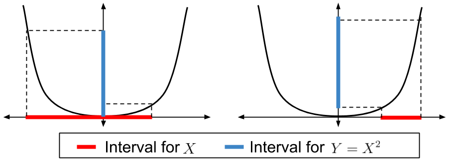
Figure 2: Two separate examples that show how interval propagation can be used to map confidence intervals for $X$ (in red) to confidence intervals for $Y=X^{2}$ (in blue).

In the following theorem, we prove that the resulting confidence interval, $\mathcal{C}$, has guaranteed coverage, i.e., that it holds with probability $1-\delta$.

Theorem 4 (Guaranteed coverage).

Under ass:supp, if $(\delta_{1}+\delta_{2}+\delta_{3}+\delta_{4})\leq\delta$, then for the confidence interval $\mathcal{C}\coloneqq[v^{\texttt{lb}},v^{\texttt{ub}}]$,

$$\Pr\left(\sigma^{2}(\pi)\in\mathcal{C}\right)\geq 1-\delta.$$ (12)

thm:HCOVE1

Remark 3.

thm:HCOVE1 presents a two-sided interval. If only a lower bound or only an upper bound is required, then it suffices if only $(\delta_{1}+\delta_{2})\leq\delta$ or $(\delta_{3}+\delta_{4})\leq\delta$, respectively.

Remark 4.

$\mathcal{C}$ can always be clipped via taking the intersection with the interval $[0,(G_{\texttt{max}}-G_{\texttt{min}})^{2}/4]$, since the variance will always be within this range (see Popoviciu’s inequality for the deterministic upper bound on variance).

A Tale of Long-Tails

One important advantage of thm:HCOVE1 is that it constructs a CI, $\mathcal{C}$, for $\sigma^{2}(\pi)$ using any concentration inequality that can be used to get CIs $\operatorname{CI}_{+}(\mathbb{E}_{\beta}[\rho G])$ and $\operatorname{CI}_{-}(\mathbb{E}_{\beta}[\rho G])$) for $\mu(\pi)$. Hence, the tightness of $\mathcal{C}$ scales directly with the tightness of these existing off-policy policy evaluation methods for the expected discounted return. However, naïvely using common concentration inequalities can result in wide and uninformative CIs, as we discuss below. Therefore, in this section, we aim to establish a control-variate that is designed to produce tighter CIs for $\sigma^{2}(\pi)$.

Typically, for a random variable $X\in[a,b]$, the width of the confidence interval for $\mathbb{E}[X]$ obtained using common concentration inequalities, like Hoeffding’s (Hoeffding 1994) or an empirical Bernstein inequality (Maurer and Pontil 2009), have a direct dependence on the range, $(b-a)$. Unfortunately, as shown by Thomas, Theocharous, and Ghavamzadeh (2015), IS based estimators may exhibit extremely long tail behavior and can have a range in the order of $10^{10}$. For example, even if $\forall a\in\mathcal{A}$ and $\forall s\in\mathcal{S}$, if $\beta(a|s)>0.1$, then the maximum possible importance weighted return of a ten timestep long trajectory can be on the order of $(1/0.1)^{10}=10^{10}$ even when returns are normalized to the $[0,1]$ interval. Such a large range causes Hoeffding’s inequality and empirical Bernstein inequalities to produce wide and uninformative confidence intervals, especially when the number of samples is not enormous.

To construct a lower bound for $\mathbb{E}[X]$, while being robust to the long tail, Thomas, Theocharous, and Ghavamzadeh (2015) notice that truncating the upper-tail of $X$ to a constant $c$ can only lower the expected value of $X$, i.e., for $X^{\prime}\coloneqq\texttt{min}(X,c),\,\,\mathbb{E}[X^{\prime}]\leq\mathbb{E}[X]$. Therefore, $X_{\texttt{lb}}^{\prime}\coloneqq\operatorname{CI}_{-}(\mathbb{E}[X^{\prime}],\delta)$ is also a valid lower bound for $\mathbb{E}[X]$ and $\Pr(X_{\texttt{lb}}^{\prime}\leq\mathbb{E}[X])\geq 1-\delta$. Additionally, truncating allows for significantly shrinking the range from $[a,b]$ to $[a,c]$, thereby effectively leading to a much tighter lower bound when $c$ is chosen appropriately. For completeness, we review this bound in Appendix F.

While this bound was designed specifically for getting the lower bounds required in (9) and (10), it cannot be naïvely used to get the upper bounds. As $\mathbb{E}[X^{\prime}]\leq\mathbb{E}[X]$, the upper bound $X_{\texttt{ub}}^{\prime}\coloneqq\operatorname{CI}^{+}(\mathbb{E}[X^{\prime}],\delta)$, may not be a valid upper bound for $\mathbb{E}[X]$ and $\Pr(X_{\texttt{ub}}^{\prime}\geq\mathbb{E}[X])\not\geq 1-\delta$. A natural question is then: How can an upper bound be obtained that is robust to the long upper tail?

To answer this question, notice that if instead of the upper tail, the lower tail of the distribution was long, then the upper bound constructed after truncating the lower tail would still be valid. Therefore, we introduce a control-variate $\xi$ which can be used to switch the tails of the distribution of an IS based estimator, such that both upper and lower valid bounds can be obtained using the resulting distribution. We formalize this in the following theorem.

Theorem 5.

Let $X$ be either $G$ or $G^{2}$, then for any $\delta\in(0,0.5]$ and a fixed constant $\xi$,

$$\operatorname{CI}^{+}_{-}(\mathbb{E}_{\beta}[\rho X],\delta)=\operatorname{CI}^{+}_{-}(\mathbb{E}_{\beta}[\rho(X-\xi)],\delta)+\xi.$$ (13)

prop:control

Remark 5.

When $\xi$ is set to be the maximum value that $X$ can take, then the random variable $\rho(X-\xi)$ will have an upper bound of $0$ and a long lower tail since $\rho\geq 0$ and $(X-\xi)\leq 0$. Similarly, when $\xi$ is set to be the minimum value that $X$ can take, then the random variable $\rho(X-\xi)$ will have a lower bound of $0$ and a long upper tail. When a two-sided interval is required, two different estimators need to be constructed using the values for $\xi$ discussed above.

prop:control allows us to control the tail-behavior such that the tight bounds presented by Thomas, Theocharous, and Ghavamzadeh (2015) can be leveraged to obtain both valid upper and valid lower high-confidence bound. However, prop:control still makes use of the full trajectory importance ratio $\rho$, which can result in high-variance and inflate the confidence intervals.

To mitigate the above problem as well, we combine the variance reduction property of per-decision and coupled-decision IS offered by thm:cdis, and the control over the tail behavior offered by prop:control, and present the following theorem (see Appendix F for the complete algorithm).

Theorem 6.

Under ass:supp, for any $\delta\in[0.0.5]$, let $\xi_{R}\coloneqq\texttt{max}(R_{\texttt{min}}^{2},R_{\texttt{max}}^{2})$ and $\xi_{G}\coloneqq\texttt{max}(G_{\texttt{min}}^{2},G_{\texttt{max}}^{2})$ then

$$X\coloneqq \sum_{i=0}^{T}\sum_{j=0}^{T}\rho\left(0,\texttt{max}(i,j)\right)\gamma^{i+j}\left(R_{(i)}R_{(j)}-\xi_{R}\right),$$ (14)

$$Y\coloneqq \sum_{i=0}^{T}\rho(0,i)\gamma^{i}\left(R_{(i)}-R_{\texttt{max}}\right),$$ (15)

then $\Pr(X\leq 0)=\Pr(Y\leq 0)=1$, and

$$\operatorname{CI}^{+}\left(\mathbb{E}_{\beta}[\rho G^{2}],\delta\right) =\operatorname{CI}^{+}\left(\mathbb{E}_{\beta}[X],\delta\right)+\xi_{G},$$ (16)

$$\operatorname{CI}^{+}\left(\mathbb{E}_{\beta}[\rho G],\delta\right) =\operatorname{CI}^{+}\left(\mathbb{E}_{\beta}[Y],\delta\right)+G_{\texttt{max}}.$$ (17)

Remark 6.

For a lower bound on $\mathbb{E}_{\beta}[\rho G^{2}]$, notice that $\rho G^{2}\geq 0$ always and thus the lower bound on $\mathbb{E}_{\beta}[X]$, where $\xi_{R}$ and $\xi_{G}$ are set to $0$, can be used. Lower bound on $\mathbb{E}_{\beta}[\rho G]$ can be constructed by using the lower bound on $\mathbb{E}_{\beta}[Y]$, when $R_{\texttt{max}}$ and $G_{\texttt{max}}$ are replaced by $R_{\texttt{min}}$ and $G_{\texttt{min}}$.

Remark 7.

If some trajectories have horizon length $t<T$, then they must be appropriately padded to ensure that $\forall i\in[t+1,T],\,\,\rho(0,i)=\rho(0,t)$ and $R_{(i)}=0$, such that in expectation the total amount added/subtracted by the control variate is zero.

HCOVE using Statistical Bootstrapping

Bootstrap is a popular non-parametric technique for finding approximate confidence intervals (Efron and Tibshirani 1994). The core idea of bootstrap is to re-sample the observed data $\mathcal{D}$ and construct $B$ pseudo-datasets $\{\mathcal{D}^{*}_{i}\}_{i=1}^{B}$ in a way such that each $\mathcal{D}^{*}_{i}$ resembles a draw from the true underlying data generating process. With each pseudo-data $\mathcal{D}_{i}$, an unbiased pseudo-estimate of a desired sample statistic can be created. For our problem, this statistic corresponds to $\hat{\sigma}_{n}^{2*}$, the estimate of $\sigma^{2}(\pi)$ obtained using (7). Thereby, leveraging the entire set of pseudo-data $\{\mathcal{D}^{*}_{i}\}_{i=1}^{B}$, an empirical distribution for the estimates of the variance $\{\hat{\sigma}^{2*}_{n,i}\}_{i=1}^{B}$ can be obtained. This empirical distribution approximates the true distribution of $\hat{\sigma}_{n}^{2}$ and can thus be leveraged to obtain CIs for $\sigma^{2}(\pi)$ using the percentile method, the bias-corrected and accelerated (BCa) method, etc. (DiCiccio and Efron 1996).

A drawback of bootstrap is the increased computational cost required for re-sampling and analysing $B$ pseudo data-sets. Further, the CIs obtained from bootstrap are only approximate, meaning that they can fail with more than $\delta$ probability. However, the primary advantage of using bootstrap is that it provides much tighter CIs, as compared to the ones obtained using concentration inequalities, and hence can be more informative for certain applications in practice.

Let $\hat{\mathcal{C}}$ be the approximate interval for $\sigma^{2}(\pi)$, for a given confidence $\delta$, obtained using bootstrap (see Appendix F for the complete algorithm). Then under the following assumption on the higher-moments of $\hat{\sigma}_{n}^{2}$, we directly leverage the results for bootstrap to obtain an error-rate for $\hat{\mathcal{C}}$.

Assumption 2.

The third moment of $\hat{\sigma}_{n}^{2}$ is bounded. That is, $\exists c_{1}<\infty$ such that $\mathbb{E}_{\beta}[(\hat{\sigma}_{n}^{2}-\mathbb{E}_{\beta}[\hat{\sigma}_{n}^{2}])^{3}]<c_{1}$. ass:bounded

ass:bounded is a typical requirement for bootstrap methods (Efron and Tibshirani 1994). ass:bounded can easily be satisfied by commonly used entropy regularized behavior policies that ensure that $\exists c_{2}>0$ such that $\forall a\in\mathcal{A},\forall s\in\mathcal{S},\,\,\beta(a|s)\geq c_{2}$. This would ensure that the importance ratio $\rho\leq 1/(c_{2}^{T})$ , and because $G\leq G_{\texttt{max}}$, $\rho G$ and $\rho G^{2}$ would also be bounded. This ensures that $\hat{\sigma}_{n}^{2}$ is bounded, and therefore all its moments are also bounded, as required by ass:bounded. We formalize the asymptotic correctness of bootstrap confidence intervals in the following theorem.

Theorem 7.

Under ass:supp,ass:bounded, the confidence interval $\hat{\mathcal{C}}$ has a finite sample error of $O(n^{-1/2})$. That is,

$$\Pr\left(\sigma^{2}(\pi)\in\hat{\mathcal{C}}\right)\geq 1-\delta-O\left(n^{-\frac{1}{2}}\right).$$ (18)

thm:boot

Remark 8.

Other variants of bootstrap (Bootstrap-t, BCa, etc.) can also be used, which typically offer higher order refinement by reducing the finite sample error-rate to $O(n^{-1})$ (DiCiccio and Efron 1996).

Related Work

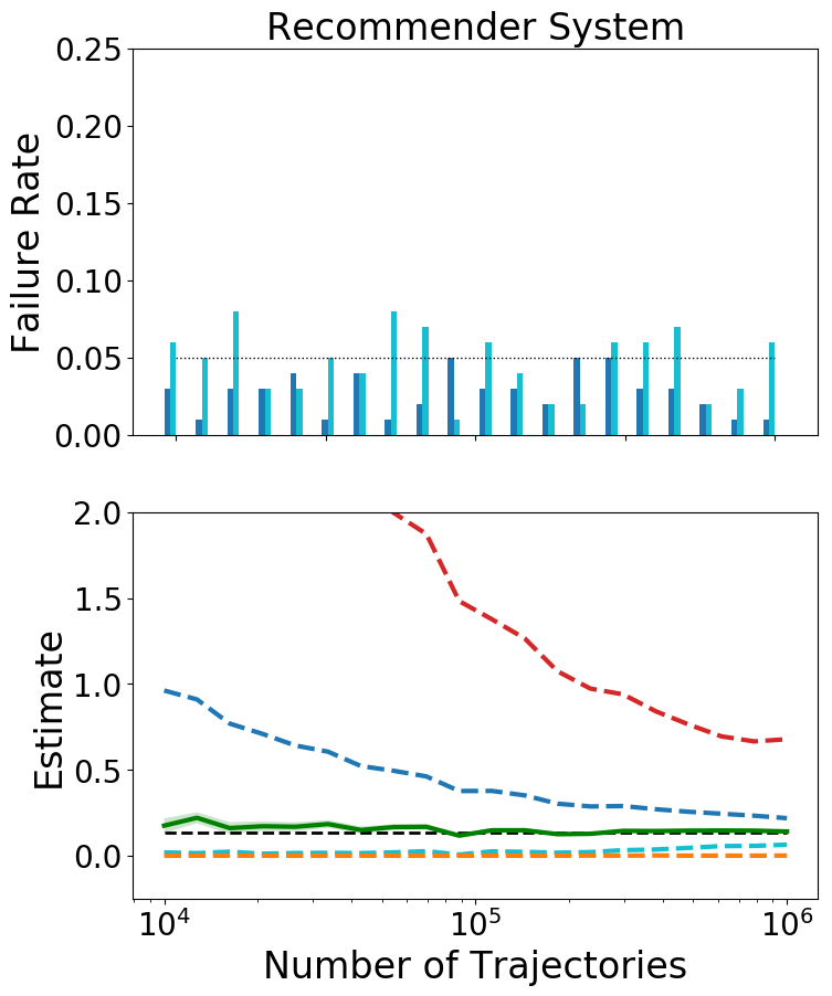
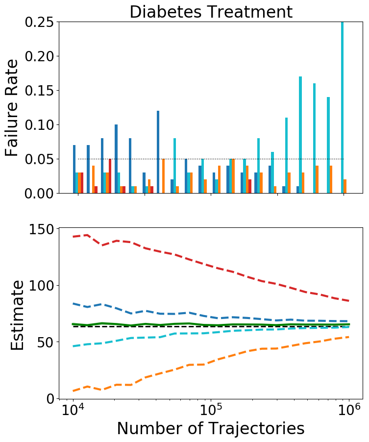
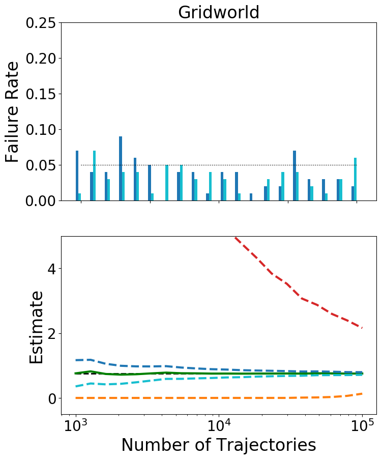
Figure 3: Experimental results using $100$ trials. (Top) Empirically observed fraction (out of 100 trials) for which the computed confidence interval did not include the actual variance, for the given number of trajectories (plotted on the shared horizontal axis), for the proposed upper and lower high-confidence bounds that were constructed using concentration inequalities (labeled as: $\operatorname{CI}+$, and $\operatorname{CI}-$) and using bootstrap (labeled as: Bootstrap $+$, and Bootstrap $-$). The color of the bars refer to the legend, and these bars should ideally be below the line representing the confidence level $\delta=0.05$. (Bottom) The dashed, colored, lines represent the value of the respective high-confidence bounds, constructed with confidence level $1-\delta$ each. The green line represents the value of our proposed estimator $\hat{\sigma}_{n}^{2}$ and the shaded area around it (almost negligible) corresponds to the standard error. Black dashed line represents the true variance, $\sigma^{2}(\pi)$. The unbiased and consistent property of $\hat{\sigma}_{n}^{2}$ can be visualized by comparing it with $\sigma^{2}(\pi)$. Notice that as the bootstrap confidence interval $\hat{\mathcal{C}}$ is only approximate, it can fail with more that $\delta$ probability. In comparison, confidence interval $\mathcal{C}$ obtained using concentration inequalities provide guaranteed coverage. However, as clear from the plots, $\mathcal{C}$ can be conservative, while $\hat{\mathcal{C}}$ provides a tighter interval.

When samples are from the distribution whose variance needs to be estimated, then under the assumption that the distribution is normal, the $\chi^{2}$ distribution can be used for providing CIs for the variance. Effects of non-normality on tests of significance were first analyzed by Pearson and Adyanthaya (1929) and has led to a large body of literature on variance tests (Pearson 1931; Box 1953; Levene 1960). Various modifications to $\chi^{2}$ tests have also been proposed to be robust against samples from non-normal distributions (Subrahmaniam 1966; García-Pérez 2006; Pan 1999; Lim and Loh 1996). The statistical bootstrap approach used in this paper to obtain bounds on the variance is closest to the bootstrap test developed by Shao (1990). However, all of these methods are analogous to on-policy variance analysis.

In the context of RL, Sobel (1982) first introduced Bellman operators for the second moment and combined it with the first moment to compute the variance. Temporal difference (TD) style algorithms have been subsequently developed for estimating the variance of returns (Tamar, Di Castro, and Mannor 2016; La and Ghavamzadeh 2013; White and White 2016; Sherstan et al. 2018). However, such TD methods might suffer from potential instabilities when used with function approximators and off-policy data (Sutton and Barto 2018). Policy gradient style algorithms have also been developed for finding policies that optimize variance related objectives (Di Castro, Tamar, and Mannor 2012; Tamar and Mannor 2013), however, these are limited to the on-policy setting. We are not aware of any work in the RL literature that provides unbiased and consistent off-policy variance estimators, nor high-confidence bounds for thereon.

Outside RL, variants of off-policy (or counterfactual) estimation using importance sampling (or inverse propensity estimator (Horvitz and Thompson 1952)) is common in econometrics (Hoover 2011; Stock and Watson 2015) and causal inference (Pearl 2009). While these works have mostly focused on mean estimation, counterfactual probability density or quantiles of potential outcomes can also be estimated (DiNardo, Fortin, and Lemieux 1995; Melly 2006; Chernozhukov, Fernández-Val, and Melly 2013; Donald and Hsu 2014). Such distribution estimation methods can possibly also be used to estimate off-policy variance; however it is unclear how to obtain unbiased estimates of the variance from an unbiased estimate of the distribution. Instead, focusing directly on the variance can be more data-efficient and can also lead to unbiased estimators. Further, these works neither leverage any MDP structure to reduce variance resulting from IS, nor do they provide any methods that provide high-confidence bounds on the variance. In the RL setting, the problem of high variance in IS is exacerbated as sequential interaction leads to multiplicative importance ratios, thereby requiring additional consideration for long tails to obtain tight bounds.

Experimental Study

Inspired by real-world applications where OVE and HCOVE can be useful, we validate our proposed estimators empirically on two domains motivated by real-world applications. Here, we only provide a brief description about the experimental setup and the main results. Appendix G contains additional experimental details.

Diabetes treatment: This domain is based on an open-source implementation (Xie 2019) of the FDA approved Type-1 Diabetes Mellitus simulator (T1DMS) (Man et al. 2014) for treatment of Type-1 Diabetes, where the objective is to control an insulin pump to regulate the blood-glucose level of a patient. High-confidence estimation of the variance of a controller’s outcome, before deployment, can be informative when assessing potential harm to the patient that may be caused by the controller.

Recommender system: This domain simulates the problem of providing online recommendations based on customer interests, where it is often useful to obtain high-confidence estimates for the variance of customer’s experience, before actually deploying the system, to limit financial loss.

Gridworld: We also consider a standard $4\times 4$ Gridworld with stochastic transitions. There are eight discrete actions corresponding to up, down, left, right, and the four diagonal movements.

Given trajectories collected using a behavior policy $\beta$, in Figure 3 we provide the trend of our estimator $\hat{\sigma}_{n}^{2}$ for an evaluation policy $\pi$, and the confidence intervals $\mathcal{C}$ and $\hat{\mathcal{C}}$ as the number of trajectories increase (more details on how $\pi$ and $\beta$ were constructed can be found in Appendix G). As established in thm:unbiased and thm:consistent, $\hat{\sigma}_{n}^{2}$ can be seen to be both an unbiased and a consistent estimator of $\sigma^{2}(\pi)$. Similarly, as established in thm:HCOVE1, the $(1-\delta)$-confidence interval $\mathcal{C}$ provides guaranteed coverage. In comparison, as established in thm:boot, bootstrap bounds are approximate and can fail more than $\delta$ fraction of the time. However, bootstrap bounds can still be useful in many applications as they provide tighter intervals.

Conclusion

In this work, we addressed an understudied problem of estimating and bounding $\sigma^{2}(\pi)$ using only off-policy data. We took the first steps towards developing a model-free, off-policy, unbiased, and consistent estimator of $\sigma^{2}(\pi)$ using a simple double-sampling trick. We then showed how bound propagation using concentration inequalities, or statistical bootstrap, can be used to obtain CIs for $\sigma^{2}(\pi)$. Finally, empirical results were provided to support the established theoretical results.

Broader Impact

Note to a wider audience:

Methods developed in this work can be beneficial for researchers and practitioners working with applications that require reliability guarantees, especially before the proposed system/policy is even deployed. It is worth noting that if the failure rate $\delta$ is set to be too low, then our bounds can result in overly conservative intervals. Further, for settings where the probabilities from behavior policies are not available, and are instead estimated, $\hat{\sigma}_{n}$ might be biased. Consequently, for applications that require hard-guarantees, or have a batch of sampled actions without their sampling probabilities, our methods are not applicable.

Future research directions:

While we took some measures to mitigate the variance of $\hat{\sigma}_{n}$, IS can still result in high variance. Recent off-policy mean estimation methods show how the Markov structure of an MDP (Liu et al. 2018; Xie, Ma, and Wang 2019; Rowland et al. 2020) or an estimate of the model of an MDP (Jiang and Li 2016; Thomas and Brunskill 2016) can be further leveraged for variance reduction. Alternatively, if the entire behavior policy is available, and not just the probabilities for the sampled actions, then multi-importance sampling (Sbert, Havran, and Szirmay-Kalos 2018) can be leveraged to relax ass:supp and also get tighter bounds on the mean return (Papini et al. 2019; Metelli et al. 2020). Extending these methods for OVE and HCOVE remains an interesting future direction.

High-Confidence Off-Policy (or Counterfactual) Variance Estimation
(Supplementary Material)

Appendix A A: Proofs for the Naïve Estimator $\hat{\sigma}_{n}^{2!!}$

Property 1.

Under ass:supp, $\hat{\sigma}_{n}^{2!!}$ may be a biased estimator of $\sigma^{2}(\pi)$. That is, it is possible that $\mathbb{E}_{\beta}[\hat{\sigma}_{n}^{2!!}]\neq\sigma^{2}(\pi)$.

Proof.

We prove this using a counter-example. Consider the MDP shown in Figure 4.

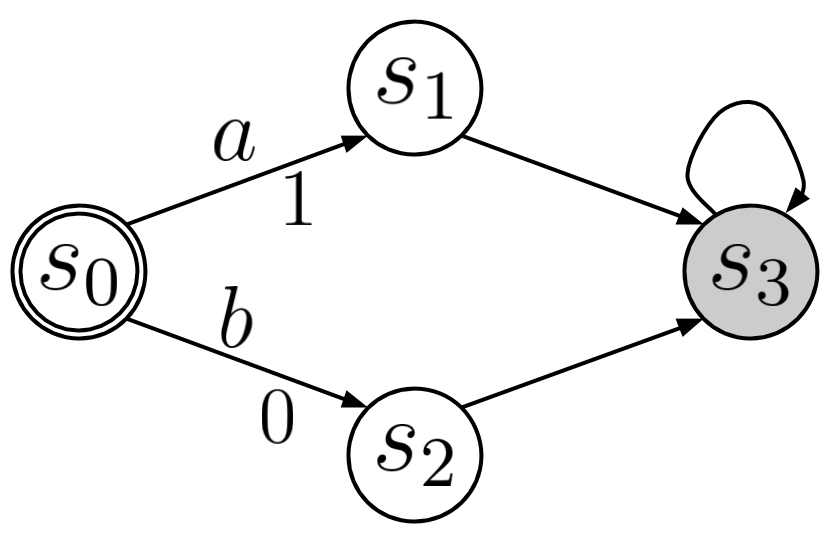
Figure 4: In this MDP, $S_{0}$ is the starting state and $S_{3}$ is the terminal/absorbing state. From $S_{0}$ there are two available actions: $a$ and $b$, which yield a reward of $1$ and $0$ respectively. All transitions are deterministic and $\gamma=1$.

For the purpose of a counter-example, we now describe the evaluation policy $\pi$ and behavior policy $\beta$. Let $\pi$ be a policy that always selects action $a$, i.e, $\pi(a|S_{0})=1$ and $\pi(b|S_{0})=0$. Since $\pi$ is deterministic and action $a$ yields a reward of $1$ always, the variance of returns observed under $\pi$ is $0$. Let $\beta$ be the behavior policy which selects both actions with equal probability, i.e., $\beta(a|S_{0})=\beta(b|S_{0})=0.5$

Now, to show that $\hat{\sigma}_{n}^{2!!}$ can be a biased estimator, we explicitly compute $\mathbb{E}[\hat{\sigma}_{n}^{2!!}]$ for the above setting, when $n=2$. The set of possible actions chosen by $\beta$ when $n=2$ can be $\{(a,a),(a,b),(b,a),(b,b)\}$, each of which is equally likely and occurs with probability of $1/4$. Before computing variance using each of these possible outcomes, recall from (3),

$$\hat{\sigma}_{n}^{2!!} =\frac{1}{n-1}\sum_{i=1}^{n}\left(\rho_{i}G_{i}-\frac{1}{n}\sum_{j=1}^{n}\rho_{j}G_{j}\right)^{2}.$$ (19)

For the case where sampled actions are $(a,a)$, the importance ratio are $(2,2)$ and

$$\hat{\sigma}_{n}^{2!!}=\frac{2}{2-1}\left(2\times 1-\frac{1}{2}(2\times 1+2\times 1)\right)^{2}=0.$$ (20)

Similarly, for the cases where sampled actions are $(a,b)$ or $(b,a)$, the importance ratios are $(2,0)$ or $(0,2)$ respectively, and

$$\hat{\sigma}_{n}^{2!!}=\frac{(2\times 1-\frac{1}{2}(2\times 1+0))^{2}+(0-\frac{1}{2}(0+2\times 1))^{2}}{2-1}=1+1=2.$$ (21)

For the cases where sampled actions are $(b,b)$ the importance ratios are $(0,0)$ respectively, and $\hat{\sigma}_{n}^{2!!}=0$. Therefore, the expected value of $\hat{\sigma}_{n}^{2!!}=\frac{1}{4}(0+2+2+0)=1\neq 0$, and it is a biased estimator.

∎

Property 2.

Under ass:supp, $\hat{\sigma}_{n}^{2!!}$ may not be a consistent estimator of $\sigma^{2}(\pi)$. That is, it is not always the case that $\hat{\sigma}_{n}^{2!!}\overset{\text{a.s}}{\longrightarrow}\sigma^{2}(\pi)$.

Proof.

We begin by expanding (3),

$$\lim_{n\rightarrow\infty}\hat{\sigma}_{n}^{2!!} =\lim_{n\rightarrow\infty}\frac{1}{n-1}\sum_{i=1}^{n}\left(\rho_{i}G_{i}-\frac{1}{n}\sum_{j=1}^{n}\rho_{j}G_{j}\right)^{2}$$ (22)

$$=\lim_{n\rightarrow\infty}\frac{1}{n-1}\sum_{i=1}^{n}\left(\rho_{i}^{2}G_{i}^{2}-\frac{2}{n}(\rho_{i}G_{i})\sum_{j=1}^{n}\rho_{j}G_{j}+\left(\frac{1}{n}\sum_{j=1}^{n}\rho_{j}G_{j}\right)^{2}\right)$$ (23)

$$=\lim_{n\rightarrow\infty}\left(\frac{1}{n-1}\sum_{i=1}^{n}\rho_{i}^{2}G_{i}^{2}-2\left(\frac{1}{n-1}\sum_{i=1}^{n}\rho_{i}G_{i}\right)\left(\frac{1}{n}\sum_{j=1}^{n}\rho_{j}G_{j}\right)+\frac{1}{n-1}\sum_{i=1}^{n}\left(\frac{1}{n}\sum_{j=1}^{n}\rho_{j}G_{j}\right)^{2}\right).$$ (24)

Notice, (a) $1/(n-1)=(1/n)(n/(n-1))$ and in the limit $n/(n-1)\rightarrow 1$, therefore $1/(n-1)\rightarrow 1/n$, and (b) using Kolmogorov’s strong law of large numbers, $\frac{1}{n}\sum_{j=1}^{n}\rho_{j}G_{j}\overset{\text{a.s.}}{\rightarrow}\mathbb{E}_{\beta}[\rho G]=\mathbb{E}_{\pi}[G]$, and $\frac{1}{n}\sum_{i=1}^{n}\rho_{i}^{2}G_{i}^{2}\overset{\text{a.s.}}{\rightarrow}\mathbb{E}_{\beta}[\rho^{2}G^{2}]=\mathbb{E}_{\pi}[\rho G^{2}]$. Therefore using Slutsky’s theorem, (24) can be simplified to,

$$\lim_{n\rightarrow\infty}\hat{\sigma}_{n}^{2!!} \overset{\text{a.s.}}{\longrightarrow}\mathbb{E}_{\pi}\left[\rho G^{2}\right]-\mathbb{E}_{\pi}[G]^{2}.$$ (25)

Since $\sigma^{2}(\pi)=\mathbb{V}_{\pi}(G)=\mathbb{E}_{\pi}\left[G^{2}\right]-\mathbb{E}_{\pi}[G]^{2}$, (25) may not be equal to $\sigma^{2}(\pi)$.

∎

Appendix B B: Proofs for the Naïve Estimator $\hat{\sigma}_{n}^{2!}$

Property 3.

Under ass:supp, $\hat{\sigma}_{n}^{2!}$ may be a biased estimator of $\sigma^{2}(\pi)$. That is, it is possible that $\mathbb{E}_{\beta}[\hat{\sigma}_{n}^{2!}]\neq\sigma^{2}(\pi)$.

Proof.

This proof uses the same counter-example presented in the proof of prop:naive1biased. Recall from (5) that,

$$\hat{\sigma}_{n}^{2!} =\frac{1}{n-1}\sum_{i=1}^{n}\rho_{i}\left(G_{i}-\frac{1}{n}\sum_{j=1}^{n}\rho_{j}G_{j}\right)^{2}$$ (26)

For the case where sampled actions are $(a,a)$, the importance ratios are $(2,2)$ and

$$\hat{\sigma}_{n}^{2!}=\frac{2}{2-1}\left(2\times\left(1-\frac{1}{2}(2\times 1+2\times 1)\right)^{2}\right)=4.$$ (27)

Similarly, for the cases where sampled actions are $(a,b)$ or $(b,a)$, the importance ratios are $(2,0)$ or $(0,2)$ respectively, and

$$\hat{\sigma}_{n}^{2!}=\frac{(2\times(1-\frac{1}{2}(2\times 1+0))^{2})+(0\times(0-\frac{1}{2}(2\times 1+0))^{2})}{2-1}=0+0=0.$$ (28)

For the cases where sampled actions are $(b,b)$ the importance ratios are $(0,0)$ respectively, and $\hat{\sigma}_{n}^{2!}=0$. Therefore, the expected value of $\hat{\sigma}_{n}^{2!}=\frac{1}{4}(4+0+0+0)=1\neq 0$, and it is a biased estimator. ∎

Property 4.

Under ass:supp, $\hat{\sigma}_{n}^{2!}$ is a consistent estimator of $\sigma^{2}(\pi)$. That is, $\hat{\sigma}_{n}^{2!}\overset{\text{a.s.}}{\longrightarrow}\sigma^{2}(\pi)$.

Proof.

We begin by expanding (3),

$$\lim_{n\rightarrow\infty}\hat{\sigma}_{n}^{2!!} =\lim_{n\rightarrow\infty}\frac{1}{n-1}\sum_{i=1}^{n}\rho_{i}\left(G_{i}-\frac{1}{n}\sum_{j=1}^{n}\rho_{j}G_{j}\right)^{2}$$ (29)

$$=\lim_{n\rightarrow\infty}\frac{1}{n-1}\sum_{i=1}^{n}\left(\rho_{i}G_{i}^{2}-\frac{2}{n}(\rho_{i}G_{i})\sum_{j=1}^{n}\rho_{j}G_{j}+\rho_{i}\left(\frac{1}{n}\sum_{j=1}^{n}\rho_{j}G_{j}\right)^{2}\right)$$ (30)

$$=\lim_{n\rightarrow\infty}\left(\frac{1}{n-1}\sum_{i=1}^{n}\rho_{i}G_{i}^{2}-2\left(\frac{1}{n-1}\sum_{i=1}^{n}\rho_{i}G_{i}\right)\left(\frac{1}{n}\sum_{j=1}^{n}\rho_{j}G_{j}\right)+\left(\frac{1}{n-1}\sum_{i=1}^{n}\rho_{i}\right)\left(\frac{1}{n}\sum_{j=1}^{n}\rho_{j}G_{j}\right)^{2}\right).$$ (31)

Notice, (a) $1/(n-1)=(1/n)(n/(n-1))$ and in the limit $n/(n-1)\rightarrow 1$, therefore $1/(n-1)\rightarrow 1/n$, and (b) using Kolmogorov’s strong law of large numbers, $\frac{1}{n}\sum_{j=1}^{n}\rho_{i}G_{i}\overset{\text{a.s.}}{\rightarrow}\mathbb{E}_{\beta}[\rho G]=\mathbb{E}_{\pi}[G]$, further $\frac{1}{n}\sum_{j=1}^{n}\rho_{i}G_{i}^{2}\overset{\text{a.s.}}{\rightarrow}\mathbb{E}_{\beta}[\rho G^{2}]=\mathbb{E}_{\pi}[G^{2}]$, and $\frac{1}{n}\sum_{i=1}^{n}\rho_{i}\overset{\text{a.s.}}{\rightarrow}\mathbb{E}_{\beta}[\rho]=1$. Therefore using Slutsky’s theorem, (31) can be simplified to,

$$\lim_{n\rightarrow\infty}\hat{\sigma}_{n}^{2!!} \overset{\text{a.s.}}{\longrightarrow}\mathbb{E}_{\pi}\left[G_{i}^{2}\right]-\mathbb{E}_{\pi}[G]^{2}$$ (32)

$$=\mathbb{V}_{\pi}(G)$$ (33)

$$=\sigma^{2}(\pi).$$ (34)

∎

Appendix C C: Proofs for the Proposed Estimator $\hat{\sigma}_{n}^{2}$

Theorem 1.

Under ass:supp, $\hat{\sigma}_{n}^{2}$ is an unbiased estimator of $\sigma^{2}(\pi)$. That is, $\mathbb{E}_{\beta}[\hat{\sigma}_{n}^{2}]=\sigma^{2}(\pi)$.

Proof.

$$\mathbb{E}_{\beta}[\hat{\sigma}_{n}^{2}] =\mathbb{E}_{\beta}\left[\frac{1}{n}\sum_{i=1}^{n}\rho_{i}G_{i}^{2}-\left(\frac{1}{|\mathcal{D}_{1}|}\sum_{i=1}^{|\mathcal{D}_{1}|}\rho_{i}G_{i}\right)\left(\frac{1}{|\mathcal{D}_{2}|}\sum_{i=1}^{|\mathcal{D}_{2}|}\rho_{i}G_{i}\right)\right]$$ (35)

$$=\mathbb{E}_{\beta}\left[\frac{1}{n}\sum_{i=1}^{n}\rho_{i}G_{i}^{2}\right]-\mathbb{E}_{\beta}\left[\left(\frac{1}{|\mathcal{D}_{1}|}\sum_{i=1}^{|\mathcal{D}_{1}|}\rho_{i}G_{i}\right)\right]\mathbb{E}_{\beta}\left[\left(\frac{1}{|\mathcal{D}_{2}|}\sum_{i=1}^{|\mathcal{D}_{2}|}\rho_{i}G_{i}\right)\right]$$ (36)

$$=\mathbb{E}_{\beta}\left[\rho G^{2}\right]-\mathbb{E}_{\beta}\left[\rho G\right]\mathbb{E}_{\beta}\left[\rho G\right]$$ (37)

$$=\mathbb{E}_{\pi}\left[G^{2}\right]-\mathbb{E}_{\pi}\left[G\right]\mathbb{E}_{\pi}\left[G\right]$$ (38)

$$=\mathbb{V}_{\pi}[G]$$ (39)

$$=\sigma^{2}(\pi).$$ (40)

Example of negative variance estimate:

For completeness, we also work out the expected estimate of $\hat{\sigma}_{n}^{2}$ for the counter-example used to show $\hat{\sigma}_{n}^{2!!}$ and $\hat{\sigma}_{n}^{2!}$ are biased. This example also shows that the $\hat{\sigma}_{n}$ can be negative. For the case where sampled actions are $(a,a)$, the importance ratio are $(2,2)$ and $\hat{\sigma}_{n}$ is negative,

$$\hat{\sigma}_{n}^{2}=\frac{1}{2}(2\times 1+2\times 1)-(2\times 1)(2\times 1)=-2.$$ (41)

Similarly, for the cases where sampled actions are $(a,b)$ or $(b,a)$, the importance ratios are $(2,0)$ or $(0,2)$ respectively, and

$$\hat{\sigma}_{n}^{2}=\frac{1}{2}(2\times 1+0)-(2\times 1)\times(0)=1.$$ (42)

For the cases where sampled actions are $(b,b)$, the importance ratios are $(0,0)$ respectively, and $\hat{\sigma}_{n}^{2}=0$. Therefore, the expected value of $\hat{\sigma}_{n}^{2}=\frac{1}{4}(-2+1+1+0)=0$, as required.

∎

Theorem 2.

Under ass:supp, $\hat{\sigma}_{n}^{2}$ is a consistent estimator of $\sigma^{2}(\pi)$. That is, $\hat{\sigma}_{n}^{2}\overset{\text{a.s.}}{\longrightarrow}\sigma^{2}(\pi)$.

Proof.

$$\lim_{n\rightarrow\infty}\hat{\sigma}_{n}^{2} =\lim_{n\rightarrow\infty}\left[\frac{1}{n}\sum_{i=1}^{n}\rho_{i}G_{i}^{2}-\left(\frac{1}{|\mathcal{D}_{1}|}\sum_{i=1}^{|\mathcal{D}_{1}|}\rho_{i}G_{i}\right)\left(\frac{1}{|\mathcal{D}_{2}|}\sum_{i=1}^{|\mathcal{D}_{2}|}\rho_{i}G_{i}\right)\right].$$ (43)

Now using Kolmogorov’s strong law of large numbers and Slutsky’s theorem, (43) can be simplified to

$$\lim_{n\rightarrow\infty} =\left[\lim_{n\rightarrow\infty}\frac{1}{n}\sum_{i=1}^{n}\rho_{i}G_{i}^{2}\right]-\left[\lim_{n\rightarrow\infty}\left(\frac{1}{|\mathcal{D}_{1}|}\sum_{i=1}^{|\mathcal{D}_{1}|}\rho_{i}G_{i}\right)\right]\left[\lim_{n\rightarrow\infty}\left(\frac{1}{|\mathcal{D}_{2}|}\sum_{i=1}^{|\mathcal{D}_{2}|}\rho_{i}G_{i}\right)\right]$$ (44)

$$\overset{\text{a.s.}}{\longrightarrow}\mathbb{E}_{\beta}\left[\rho G^{2}\right]-\mathbb{E}_{\beta}\left[\rho G\right]\mathbb{E}_{\beta}\left[\rho G\right]$$ (45)

$$=\mathbb{E}_{\pi}\left[G^{2}\right]-\mathbb{E}_{\pi}\left[G\right]\mathbb{E}_{\pi}\left[G\right]$$ (46)

$$=\mathbb{V}_{\pi}[G]$$ (47)

$$=\sigma^{2}(\pi).$$ (48)

∎

Theorem 3.

Under ass:supp,

$$\mathbb{E}_{\beta}\left[\rho G^{2}\right]=\mathbb{E}_{\beta}\left[\sum_{i=0}^{T}\sum_{j=0}^{T}\rho\left(0,\texttt{max}(i,j)\right)\gamma^{i+j}R_{(i)}R_{(j)}\right].$$ (49)

Proof.

$$\mathbb{E}_{\beta}[\rho G^{2}] =\mathbb{E}_{\beta}\left[\rho(0,T)\left(\sum_{i=0}^{T}\gamma^{i}R_{(i)}\right)^{2}\right]$$ (50)

$$=\mathbb{E}_{\beta}\left[\rho(0,T)\left(\sum_{i=0}^{T}\gamma^{2i}R_{(i)}^{2}+2\sum_{i=0}^{T}\sum_{j=i+1}^{T}\gamma^{i+j}R_{(i)}R_{(j)}\right)\right]$$ (51)

$$=\left(\sum_{i=0}^{T}\mathbb{E}_{\beta}\left[\rho(0,T)\gamma^{2i}R_{i}^{2}\right]\right)+\left(2\sum_{i=0}^{T}\sum_{j=i+1}^{T}\mathbb{E}_{\beta}\left[\rho(0,T)\gamma^{i+j}R_{(i)}R_{(j)}\right]\right)$$ (52)

$$=\sum_{i=0}^{T}\mathbb{E}_{\beta}\left[\rho(0,T)\gamma^{2i}R_{(i)}^{2}\right]+2\sum_{i=0}^{T}\sum_{j=i+1}^{T}\mathbb{E}_{\beta}\left[\rho(0,T)\gamma^{i+j}R_{(i)}R_{(j)}\right]$$ (53)

$$=\left(\sum_{i=0}^{T}\sum_{h\in\mathcal{H}_{0:T}^{\beta}}\Pr(h|\beta)\rho(0,T)\gamma^{2i}R_{(i)}^{2}\right)+\left(2\sum_{i=0}^{T}\sum_{j=i+1}^{T}\sum_{h\in\mathcal{H}_{0:T}^{\beta}}\Pr(h|\beta)\rho(0,T)\gamma^{i+j}R_{(i)}R_{(j)}\right)$$ (54)

$$\overset{(a)}{=}\left(\sum_{i=0}^{T}\sum_{h\in\mathcal{H}_{0:T}^{\pi}}\Pr(h|\pi)\gamma^{2i}R_{(i)}^{2}\right)+\left(2\sum_{i=0}^{T}\sum_{j=i+1}^{T}\sum_{h\in\mathcal{H}_{0:T}^{\pi}}\Pr(h|\pi)\gamma^{i+j}R_{(i)}R_{(j)}\right)$$ (55)

$$=\left(\sum_{i=0}^{T}\sum_{h\in\mathcal{H}_{0:i}^{\pi}}\Pr(h|\pi)\gamma^{2i}R_{(i)}^{2}\sum_{h^{\prime}\in\mathcal{H}_{i+1:t}^{\pi}}\Pr(h^{\prime}|h,\pi)\right)+\left(2\sum_{i=0}^{T}\sum_{j=i+1}^{T}\sum_{h\in\mathcal{H}_{0:j}^{\pi}}\Pr(h|\pi)\gamma^{i+j}R_{(i)}R_{(j)}\sum_{h^{\prime}\in\mathcal{H}_{j+1:t}^{\pi}}\Pr(h^{\prime}|h,\pi)\right)$$ (56)

$$=\left(\sum_{i=0}^{T}\sum_{h\in\mathcal{H}_{0:i}^{\pi}}\Pr(h|\pi)\gamma^{2i}R_{(i)}^{2}\right)+\left(2\sum_{i=0}^{T}\sum_{j=i+1}^{T}\sum_{h\in\mathcal{H}_{0:j}^{\pi}}\Pr(h|\pi)\gamma^{i+j}R_{(i)}R_{(j)}\right)$$ (57)

$$\overset{(b)}{=}\left(\sum_{i=0}^{T}\sum_{h\in\mathcal{H}_{0:i}^{\beta}}\Pr(h|\beta)\rho(0,i)\gamma^{2i}R_{(i)}^{2}\right)+\left(2\sum_{i=0}^{T}\sum_{j=i+1}^{T}\sum_{h\in\mathcal{H}_{0:j}^{\beta}}\Pr(h|\beta)\rho(0,j)\gamma^{i+j}R_{(i)}R_{(j)}\right)$$ (58)

$$=\left(\sum_{i=0}^{T}\mathbb{E}_{\beta}\left[\rho(0,i)\gamma^{2i}R_{(i)}^{2}\right]\right)+\left(2\sum_{i=0}^{T}\sum_{j=i+1}^{T}\mathbb{E}_{\beta}\left[\rho(0,j)\gamma^{i+j}R_{(i)}R_{(j)}\right]\right)$$ (59)

$$=\mathbb{E}_{\beta}\left[\sum_{i=0}^{T}\rho(0,i)\gamma^{2i}R_{(i)}^{2}+2\sum_{i=0}^{T}\sum_{j=i+1}^{T}\rho(0,j)\gamma^{i+j}R_{(i)}R_{(j)}\right]$$ (60)

$$=\mathbb{E}_{\beta}\left[\sum_{i=0}^{T}\sum_{j=0}^{T}\rho\left(0,\texttt{max}(i,j)\right)\gamma^{i+j}R_{(i)}R_{(j)}\right],$$ (61)

where steps (a) and (b) follow due to ass:supp. ∎

Appendix D Proofs for HCOVE using Concentration Inequalities

Theorem 4.

Under ass:supp, if $(\delta_{1}+\delta_{2}+\delta_{3}+\delta_{4})\leq\delta$, then for the confidence interval $\mathcal{C}\coloneqq[v^{\texttt{lb}},v^{\texttt{ub}}]$,

$$\Pr\left(\sigma^{2}(\pi)\in\mathcal{C}\right)\geq 1-\delta.$$ (62)

Proof.

For brevity, let $X\coloneqq\mathbb{E}_{\beta}[\rho G^{2}],\text{and}\,\,Y\coloneqq\mathbb{E}_{\beta}[\rho G]^{2}$.

$$\Pr(v^{\texttt{lb}}\leq\sigma^{2}(\pi)) =\Pr\left(\operatorname{CI}_{-}(X,\delta_{1})-\operatorname{CI}^{+}(Y^{2},\delta_{2})\leq X-Y\right)$$ (63)

$$\geq\Pr\left((\operatorname{CI}_{-}(X,\delta_{1})\leq X)\cap(Y\leq\operatorname{CI}^{+}(Y^{2},\delta_{2}))\right)$$ (64)

$$=1-\Pr\left(((\operatorname{CI}_{-}(X,\delta_{1})\leq X)\cap(Y\leq\operatorname{CI}^{+}(Y^{2},\delta_{2})))^{c}\right)$$ (65)

$$=1-\Pr\left((\operatorname{CI}_{-}(X,\delta_{1})\leq X)^{c}\cup(Y\leq\operatorname{CI}^{+}(Y^{2},\delta_{2}))^{c}\right)$$ (66)

$$=1-\Pr\left((\operatorname{CI}_{-}(X,\delta_{1})>X)\cup(Y>\operatorname{CI}^{+}(Y^{2},\delta_{2}))\right)$$ (67)

$$=1-\left(\delta_{1}+\delta_{2}\right),$$ (68)

where superscript of $c$ represents complement. Similarly, it can be shown that $\Pr(v^{\texttt{ub}}\geq\sigma^{2}(\pi))\geq 1-(\delta_{3}+\delta_{4})$. Therefore, the maximum probability of failure, i.e., either $v^{\texttt{ub}}<\sigma^{2}(\pi)$ or $v^{\texttt{lb}}>\sigma^{2}(\pi)$, is less than $(\delta_{1}+\delta_{2}+\delta_{3}+\delta_{4})$, which is not greater than $\delta$. ∎

Theorem 5.

Let $X$ be either $G$ or $G^{2}$, then for any $\delta\in[0,0.5]$ and a fixed constant $\xi$,

$$\operatorname{CI}^{+}_{-}(\mathbb{E}_{\beta}[\rho X],\delta)=\operatorname{CI}^{+}_{-}(\mathbb{E}_{\beta}[\rho(X-\xi)],\delta)+\xi.$$ (69)

Proof.

$$\operatorname{CI}^{+}_{-}(\mathbb{E}_{\beta}[\rho X],\delta) =\operatorname{CI}^{+}_{-}(\mathbb{E}_{\beta}[\rho X-\rho\xi+\rho\xi],\delta)$$ (70)

$$\overset{(a)}{=}\operatorname{CI}^{+}_{-}(\mathbb{E}_{\beta}[\rho(X-\xi)]+\mathbb{E}_{\beta}[\rho]\xi,\delta)$$ (71)

$$\overset{(b)}{=}\operatorname{CI}^{+}_{-}(\mathbb{E}_{\beta}[\rho(X-\xi)]+\xi,\delta)$$ (72)

$$\overset{(c)}{=}\operatorname{CI}^{+}_{-}(\mathbb{E}_{\beta}[\rho(X-\xi)],\delta)+\xi,$$ (73)

where (a) and (c) follow because $\xi$ is a fixed constant, and $(b)$ follows because $\mathbb{E}_{\beta}[\rho]=1$. ∎

Theorem 6.

Under ass:supp, for any $\delta\in[0.0.5]$, let $\xi_{R}\coloneqq\texttt{max}(R_{\texttt{min}}^{2},R_{\texttt{max}}^{2})$ and $\xi_{G}\coloneqq\texttt{max}(G_{\texttt{min}}^{2},G_{\texttt{max}}^{2})$ then

$$X\coloneqq \sum_{i=0}^{T}\sum_{j=0}^{T}\rho\left(0,\texttt{max}(i,j)\right)\gamma^{i+j}\left(R_{(i)}R_{(j)}-\xi_{R}\right),$$ (74)

$$Y\coloneqq \sum_{i=0}^{T}\rho(0,i)\gamma^{i}\left(R_{(i)}-R_{\texttt{max}}\right),$$ (75)

then $\Pr(X\leq 0)=\Pr(Y\leq 0)=1$, and

$$\operatorname{CI}^{+}\left(\mathbb{E}_{\beta}[\rho G^{2}],\delta\right) =\operatorname{CI}^{+}\left(\mathbb{E}_{\beta}[X],\delta\right)+\xi_{G},$$ (76)

$$\operatorname{CI}^{+}\left(\mathbb{E}_{\beta}[\rho G],\delta\right) =\operatorname{CI}^{+}\left(\mathbb{E}_{\beta}[Y],\delta\right)+G_{\texttt{max}}.$$ (77)

Proof.

Let $c\coloneqq(1-\gamma^{T})/(1-\gamma)$. Then $\mathbb{E}_{\beta}[x]$ is.

$$\mathbb{E}_{\beta}[X] =\mathbb{E}_{\beta}\left[\sum_{i=0}^{T}\sum_{j=0}^{T}\rho\left(0,\texttt{max}(i,j)\right)\gamma^{i+j}\left(R_{(i)}R_{(j)}\right)\right]-\mathbb{E}_{\beta}\left[\sum_{i=0}^{T}\sum_{j=0}^{T}\rho\left(0,\texttt{max}(i,j)\right)\gamma^{i+j}\left(\xi_{R}\right)\right]$$ (78)

$$\overset{(a)}{=}\mathbb{E}_{\beta}\left[\rho G^{2}\right]-\xi_{R}\sum_{i=0}^{T}\sum_{j=0}^{T}\gamma^{i+j}\mathbb{E}_{\beta}\left[\rho\left(0,\texttt{max}(i,j)\right)\right]$$ (79)

$$\overset{(b)}{=}\mathbb{E}_{\beta}\left[\rho G^{2}\right]-\xi_{R}\sum_{i=0}^{T}\gamma^{i}\sum_{j=0}^{T}\gamma^{j}$$ (80)

$$=\mathbb{E}_{\beta}\left[\rho G^{2}\right]-c^{2}\xi_{R},$$ (81)

where (a) follows from thm:cdis and (b) follows because $\mathbb{E}_{\beta}\left[\rho\left(0,\texttt{max}(i,j)\right)\right]=1$. Notice that as $c^{2}\xi_{R}$ is equivalent to $\xi_{G}$, therefore substituting it into (81) gives,

$$\operatorname{CI}^{+}\left(\mathbb{E}_{\beta}[X],\delta\right)+\xi_{G} =\operatorname{CI}^{+}\left(\mathbb{E}_{\beta}[\rho G^{2}]-\xi_{G},\delta\right)+\xi_{G},$$ (82)

$$=\operatorname{CI}^{+}\left(\mathbb{E}_{\beta}[\rho G^{2}],\delta\right).$$ (83)

Similarly,

$$\mathbb{E}_{\beta}[Y] =\mathbb{E}_{\beta}\left[\sum_{i=0}^{T}\rho(0,i)\gamma^{i}R_{(i)}\right]-\mathbb{E}_{\beta}\left[\sum_{i=0}^{T}\rho(0,i)\gamma^{i}R_{\texttt{max}}\right]$$ (84)

$$=\mathbb{E}_{\beta}\left[\rho G\right]-R_{\texttt{max}}\sum_{i=0}^{T}\gamma^{i}\mathbb{E}_{\beta}\left[\rho(0,i)\right]$$ (85)

$$\overset{(c)}{=}\mathbb{E}_{\beta}\left[\rho G\right]-cR_{\texttt{max}},$$ (86)

where (c) follows because $\mathbb{E}_{\beta}\left[\rho(0,i)\right]=1$. Further, as $cR_{\texttt{max}}=G_{\texttt{max}}$,

$$\operatorname{CI}^{+}\left(\mathbb{E}_{\beta}[Y],\delta\right)+G_{\texttt{max}} =\operatorname{CI}^{+}\left(\mathbb{E}_{\beta}\left[\rho G\right]-G_{\texttt{max}},\delta\right)+G_{\texttt{max}}.$$ (87)

$$=\operatorname{CI}^{+}\left(\mathbb{E}_{\beta}\left[\rho G\right],\delta\right).$$ (88)

∎

Appendix E E. Proofs for HCOVE using Statistical Bootstrapping

Theorem 7.

Under ass:supp,ass:bounded, the confidence interval $\hat{\mathcal{C}}$ has a finite sample error of $O(n^{-1/2})$. That is,

$$\Pr\left(\sigma^{2}(\pi)\in\hat{\mathcal{C}}\right)\geq 1-\delta-O\left(n^{-1/2}\right).$$ (89)

Proof.

This proof directly leverages the finite-sample coverage error result by Efron and Tibshirani (1994). A similar technique has been used by Kostrikov and Nachum (2020) for establishing the finite-sample coverage error of the CIs for the the mean return $\mu(\pi)$ using off-policy data. Our result is inspired by theirs and establishes finite-sample coverage error of the CIs for the variance of returns, $\sigma^{2}(\pi)$. Before proceeding, we first define some additional notation and then review Hadamard differentiability (Wasserman 2006), which is a key property for establishing the validity of bootstrap.

For brevity, let $\mathcal{H}\coloneqq\mathcal{H}_{(0):(T)}$. For a trajectory $x\in\mathcal{H}$, let $\rho(x)$ be the importance ratio of the entire trajectory, $g_{1}(x)\coloneqq G$ be the return, and $g_{2}(x)\coloneqq G^{2}$ be the return squared. Considering a finite set of possible trajectories $\mathcal{H}$, for a given set of trajectories $\mathcal{D}$, let the empirical distribution over the trajectories be,

$$d^{\mathcal{D}}(x)\coloneqq\frac{1}{|\mathcal{D}|}\sum_{h\in\mathcal{D}}\delta_{\{h=x\}}.$$ (90)

Hadamard Differentiability: Suppose $F$ is a functional mapping distributions $\mathcal{P}$ over trajectories to $\mathbb{R}$. Denote $\mathcal{P}_{L}$ as the linear space generated by $\mathcal{P}$. The functional $F$ is said to be Hadamard differentiable at $d^{\mathcal{D}}\in\mathcal{P}$ if there exists a linear functional $L_{\mathcal{D}}$ on $\mathcal{P}_{L}$ such that for any $\epsilon_{n}\rightarrow 0$ and $\{P,P_{1},P_{2},P_{3},...\}\subset\mathcal{P}_{L}$ such that $\lVert P_{n}-P\rVert_{\infty}\rightarrow 0$ and $d^{\mathcal{D}}+\epsilon_{n}P_{n}\in\mathcal{P}$,

$$\lim_{n\rightarrow\infty}\left\lvert\frac{F(d^{\mathcal{D}}+\epsilon_{n}P_{n})-F(d^{\mathcal{D}})}{\epsilon_{n}}-L_{\mathcal{D}}(P)\right\rvert=0.$$ (91)

In the following, we directly leverage the finite sample coverage error rate established for bootstrap (Efron and Tibshirani 1994) by considering the functional $F$ to be our estimator $\hat{\sigma}_{n}^{2}$ and showing that it is Hadamard differentiable for all $d^{\mathcal{D}}$. To make the dependence of $d^{\mathcal{D}}$ explicit, we write $\hat{\sigma}_{n}^{2}(d^{\mathcal{D}})$ instead of $\hat{\sigma}_{n}^{2}$. Now using (7),

$$\hat{\sigma}_{n}^{2}(d^{\mathcal{D}}+\epsilon_{n}P_{n}) =\sum_{x\in\mathcal{H}}(d^{\mathcal{D}}+\epsilon_{n}P_{n})(x)\rho(x)g_{2}(x)-\left(\sum_{x\in\mathcal{H}}(d^{\mathcal{D}_{1}}+\epsilon_{n}P_{n})(x)\rho(x)g_{1}(x)\right)\left(\sum_{y\in\mathcal{H}}(d^{\mathcal{D}_{2}}+\epsilon_{n}P_{n})(y)\rho(y)g_{1}(y)\right),$$ (92)

$$\hat{\sigma}_{n}^{2}(d^{\mathcal{D}}) =\sum_{x\in\mathcal{H}}d^{\mathcal{D}}(x)\rho(x)g_{2}(x)-\left(\sum_{x\in\mathcal{H}}d^{\mathcal{D}_{1}}(x)\rho(x)g_{1}(x)\right)\left(\sum_{y\in\mathcal{H}}d^{\mathcal{D}_{2}}(y)\rho(y)g_{1}(y)\right).$$ (93)

Using (92) and (93), as $n\rightarrow\infty$ then $\epsilon_{n}\rightarrow 0$,

$$\lim_{\epsilon_{n}\rightarrow 0}\frac{\hat{\sigma}_{n}^{2}(d^{\mathcal{D}}+\epsilon_{n}P_{n})-\hat{\sigma}_{n}^{2}(d^{\mathcal{D}})}{\epsilon_{n}}= \sum_{x\in\mathcal{H}}P_{n}(x)\rho(x)g_{2}(x)$$ (94)

$$-\sum_{x\in\mathcal{H}}\sum_{y\in\mathcal{H}}\rho(x)g_{1}(x)\rho(y)g_{1}(y)\left[d^{\mathcal{D}_{1}}(x)P_{n}(y)+d^{\mathcal{D}_{2}}(y)P_{n}(x)+\underbrace{\epsilon_{n}P_{n}(x)P_{n}(y)}_{=0\text{ as }\epsilon_{n}\rightarrow 0}\right].$$ (95)

It can be seen that (95) is linear in $P_{n}$, so there exists a linear functional $L_{\mathcal{D}}$ on $P_{L}$ such that $\hat{\sigma}_{n}^{2}(d^{\mathcal{D}})$ is Hadamard differnetiable. ∎

Appendix F F. Algorithms

In this section we present the algorithms to obtain high-confidence bounds for $\sigma^{2}(\pi)$. Algorithms 2–3 provide lower and upper bounds using concentration inequalities. Algorithm 4 provides lower and upper bounds using statistical bootstrapping. In the following, we briefly review the concentration inequality established by Thomas, Theocharous, and Ghavamzadeh (2015), which we also use in Algorithms 2–3.

Theorem 8 ((Thomas, Theocharous, and Ghavamzadeh 2015)).

Let $\{X_{i}\}_{i=1}^{n}$ be $n$ independent real-valued bounded random variables such that for each $i\in\{1,...,n\}$, we have $\Pr(0\leq X_{i})=1$ ,$\mathbb{E}[X_{i}]\leq\mu$, and the fixed real-valued threshold $c_{i}>0$. Let $\delta>0$ and $Y_{i}\coloneqq\texttt{min}(X_{i},c_{i})$.

$$\operatorname{CI}^{-}\left(\{X_{i}\}_{i=1}^{n},\delta\right)\coloneqq\left(\sum_{i=1}^{n}\frac{1}{|c_{i}|}\right)^{-1}\!\!\!\sum_{i=1}^{n}\frac{Y_{i}}{|c_{i}|}-\left(\sum_{i=1}^{n}\frac{1}{|c_{i}|}\right)^{-1}\!\!\frac{7n\ln(2/\delta)}{3(n-1)}-\left(\sum_{i=1}^{n}\frac{1}{|c_{i}|}\right)^{-1}\!\!\!\sqrt{\frac{\ln(2/\delta)}{n-1}\sum_{i,j=1}^{n}\left(\frac{Y_{i}}{|c_{i}|}-\frac{Y_{j}}{|c_{j}|}\right)^{2}}.$$ (96)

Then with probability at least $1-\delta$, we have $\mu\geq\operatorname{CI}^{-}\left(\{X_{i}\}_{i=1}^{n},\delta\right)$. thm:thomas

Similarly, let $\{A_{i}\}_{i=1}^{n}$ be $n$ independent real-valued bounded random variables where $\Pr(0\geq A_{i})=1$ and $\mathbb{E}[A_{i}]\geq\mu$, then for a fixed real-valued threshold $c_{i}<0$ and $B_{i}\coloneqq\texttt{max}(A_{i},c_{i})$, the expected value $\mathbb{E}[B_{i}]\geq\mathbb{E}[A_{i}]$. Therefore, an upper bound on $\mathbb{E}[B_{i}]$ is also an upper bound on $\mathbb{E}[A_{i}]$. Consequently, to get an upper bound on $\mathbb{E}[B_{i}]$ we flip the bound in thm:thomas (i.e., let $Y_{i}\coloneqq-B_{i}$ in (96) and then negate the resulting bound, since $\forall\nu,\,\Pr(\mathbb{E}[Y_{i}]\geq\nu)=\Pr(-\mathbb{E}[B_{i}]\geq\nu)=\Pr(\mathbb{E}[B_{i}]\leq-\nu)$).

$$\operatorname{CI}^{+}\left(\{A_{i}\}_{i=1}^{n},\delta\right)\coloneqq\left(\sum_{i=1}^{n}\frac{1}{|c_{i}|}\right)^{-1}\!\!\!\sum_{i=1}^{n}\frac{B_{i}}{|c_{i}|}+\left(\sum_{i=1}^{n}\frac{1}{|c_{i}|}\right)^{-1}\!\!\frac{7n\ln(2/\delta)}{3(n-1)}+\left(\sum_{i=1}^{n}\frac{1}{|c_{i}|}\right)^{-1}\!\!\!\sqrt{\frac{\ln(2/\delta)}{n-1}\sum_{i,j=1}^{n}\left(\frac{B_{i}}{|c_{i}|}-\frac{B_{j}}{|c_{j}|}\right)^{2}}.$$ (97)

Then with probability at least $1-\delta$, we have $\mu\leq\operatorname{CI}^{+}\left(\{A_{i}\}_{i=1}^{n},\delta\right)$. In (96), $c_{i}$’s help in truncating the upper tail of the distribution, and in (97), $c_{i}$’s help in truncating the lower tail of the distribution. Further, note the use of absolute values for $c_{i}$’s in our presentation of the bounds by Thomas, Theocharous, and Ghavamzadeh (2015); while in (97) this is redundant as $c_{i}>0$, in (96) this is important to prevent the change in sign of the random variable when normalized using $c_{i}$’s as in this equation $c_{i}<0$. For simplicity, Thomas, Theocharous, and Ghavamzadeh (2015) suggest setting a common $c$ for all $c_{i}$’s. Further, since the value of $c$ should be chosen independent of that data being analyzed, they suggest partitioning the data into two sets $\mathcal{D}_{\text{pre}}$ and $\mathcal{D}_{\text{post}}$ in the ratio $1/20:19/20$ and searching the value of $c$ that optimizes the bound on the data from $\mathcal{D}_{\text{pre}}$. The value of this $c$ is then used to get the desired bounds using data from $\mathcal{D}_{\text{post}}$. We refer the readers to the work by Thomas, Theocharous, and Ghavamzadeh (2015) for more details.

1 Input: Dataset $\mathcal{D}$, Confidence level $1-\delta$

# Upper Bound on $\mathbb{E}_{\beta}[\rho G^{2}]$

2 $\xi_{R}=\texttt{max}(R_{\texttt{min}}^{2},R_{\texttt{max}}^{2})$ and $\xi_{G}=\texttt{max}(G_{\texttt{min}}^{2},G_{\texttt{max}}^{2})$

3 $X_{i}=\sum_{j=0}^{T}\sum_{k=0}^{T}\rho_{i}\left(0,\texttt{max}(j,k)\right)\gamma^{j+k}\left(R_{i(j)}R_{i(k)}-\xi_{R}\right)$

4 $X^{\texttt{ub}}=\operatorname{CI}^{+}\left(\{X_{i}\}_{i=1}^{|\mathcal{D}|},\delta/2\right)+\xi_{G}$

5

# Upper and Lower Bounds on $\mathbb{E}_{\beta}[\rho G]$

6 $Y^{-}_{i}=\sum_{j=0}^{T}\rho_{i}(0,j)\gamma^{j}\left(R_{i(j)}-R_{\texttt{min}}\right)$,

7 $Y^{+}_{i}=\sum_{j=0}^{T}\rho_{i}(0,j)\gamma^{j}\left(R_{i(j)}-R_{\texttt{max}}\right)$,

8 $Y^{\texttt{lb}}=\operatorname{CI}^{-}\left(\{Y^{-}_{i}\}_{i=1}^{|\mathcal{D}|},\delta/4\right)+G_{\texttt{min}}$.

9 $Y^{\texttt{ub}}=\operatorname{CI}^{+}\left(\{Y^{+}_{i}\}_{i=1}^{|\mathcal{D}|},\delta/4\right)+G_{\texttt{max}}$.

10

# Lower Bound on $\mathbb{E}_{\beta}[\rho G]^{2}$ using bound propagation

11 if $Y^{\texttt{lb}}\leq 0\leq Y^{\texttt{ub}}$ then

12      $Z^{\texttt{lb}}=0$

13else

14      $Z^{\texttt{lb}}=\texttt{min}((Y^{\texttt{lb}})^{2},(Y^{\texttt{ub}})^{2})$

Return $X^{\texttt{ub}}-Z^{\texttt{lb}}$

Algorithm 2 HCOVE - upper bound (Concentration Inequality)

1 Input: Dataset $\mathcal{D}$, Confidence level $1-\delta$

# Lower Bound on $\mathbb{E}_{\beta}[\rho G^{2}]$

(Control variate is not needed as $\rho G^{2}$ is always positive.)

2 $X_{i}=\sum_{j=0}^{T}\sum_{k=0}^{T}\rho_{i}\left(0,\texttt{max}(j,k)\right)\gamma^{j+k}\left(R_{i(j)}R_{i(k)}\right)$

3 $X^{\texttt{lb}}=\operatorname{CI}^{-}\left(\{X_{i}\}_{i=1}^{|\mathcal{D}|},\delta/2\right)$

4

# Upper and Lower Bounds on $\mathbb{E}_{\beta}[\rho G]$

5 $Y^{-}_{i}=\sum_{j=0}^{T}\rho_{i}(0,j)\gamma^{j}\left(R_{i(j)}-R_{\texttt{min}}\right)$,

6 $Y^{+}_{i}=\sum_{j=0}^{T}\rho_{i}(0,j)\gamma^{j}\left(R_{i(j)}-R_{\texttt{max}}\right)$,

7 $Y^{\texttt{lb}}=\operatorname{CI}^{-}\left(\{Y^{-}_{i}\}_{i=1}^{|\mathcal{D}|},\delta/4\right)+G_{\texttt{min}}$.

8 $Y^{\texttt{ub}}=\operatorname{CI}^{+}\left(\{Y^{+}_{i}\}_{i=1}^{|\mathcal{D}|},\delta/4\right)+G_{\texttt{max}}$.

9

# Upper Bound on $\mathbb{E}_{\beta}[\rho G]^{2}$ using bound propagation

10 $Z^{\texttt{ub}}=\texttt{max}((Y^{\texttt{lb}})^{2},(Y^{\texttt{ub}})^{2})$

Return $X^{\texttt{lb}}-Z^{\texttt{ub}}$

Algorithm 3 HCOVE - lower bound (Concentration Inequality)

1 Input: Dataset $\mathcal{D}$, Confidence level $1-\delta$

2 Compute variance estimate $\hat{\sigma}_{n}^{2}=$ Algorithm 1($\mathcal{D}$)

3 Compute $B$ bootstrapped datasets $\{\mathcal{D}_{i}^{*}\}_{i=1}^{B}$

4 Compute bootstrapped variance estimates $\{\hat{\sigma}^{2*}_{n,i}\}_{i=1}^{B}$ using Algorithm 1 for $\{\mathcal{D}_{i}^{*}\}_{i=1}^{B}$.

5 Compute $\delta/2$ and $1-\delta/2$ quantiles $z_{\delta/2},z_{1-\delta/2}$ of $\{\hat{\sigma}^{2*}_{n,i}-\hat{\sigma}_{n}^{2}\}_{i=1}^{B}$

Return $\hat{\mathcal{C}}\coloneqq[\hat{\sigma}_{n}^{2}-z_{1-\delta/2},\hat{\sigma}_{n}^{2}-z_{\delta/2}]$

Algorithm 4 HCOVE - upper and lower bounds (Bootstrap)

Appendix G G. Empirical Details

In this section, we discuss domain details and how $\pi$ and $\beta$ were selected for both the domains.

Recommender System:

Online recommendation systems are popular for tutorials, movies, advertisements, etc. In all these settings it may be beneficial to assess the variability in the customer’s experience once the new system/policy is deployed. To abstract such settings, we create a simulated domain where the interest of the user for a finite set of items is represented using the reward for the corresponding item.

We use an actor-critic algorithm (Sutton and Barto 2018) to find a near optimal policy policy $\pi$, which we use as the evaluation policy. Let $\pi^{\texttt{rand}}$ be a random policy with uniform distribution over the actions (items). Then for an $\alpha=0.5$, we define the behavior policy $\beta(a|s)\coloneqq\alpha\pi(a|s)+(1-\alpha)\pi^{\texttt{rand}}(a|s)$ for all states and actions.

Gridworld:

We also consider a standard $4\times 4$ Gridworld with stochastic transitions. There are eight discrete actions corresponding to up, down, left, right, and the four diagonal movements. Behavior and the evaluation policy for this domain were obtained in a similar way as discussed for the recommender system domain.

Diabetes Treatment:

This domain is modeled using an open-source implementation (Xie 2019) of the U.S. Food and Drug Administration (FDA) approved Type-1 Diabetes Mellitus simulator (T1DMS) (Man et al. 2014) for the treatment of Type-1 diabetes. An episode corresponds to a day, and each step of an episode corresponds to a minute in an in-silico patient’s body and is governed by a continuous time non-linear ordinary differential equation (ODE) (Man et al. 2014).

To control the insulin injection, which is required for regulating the blood glucose level, we use a parameterized policy based on the amount of insulin that a person with diabetes is instructed to inject prior to eating a meal (Bastani 2014):

$$\text{injection}=\frac{\text{current blood glucose}-\text{target blood glucose}}{CF}+\frac{\text{meal size}}{CR},$$ (98)

where ‘current blood glucose’ is the estimate of the person’s current blood glucose level, ‘target blood glucose’ is the desired blood glucose, ‘meal size’ is the estimate of the size of the meal the patient is about to eat, and $CR\in[CR_{\texttt{min}},CR_{\texttt{max}}]$ and $CF\in[CF_{\texttt{min}},CF_{\texttt{max}}]$ are two real-valued parameters that must be tuned based on the body parameters to make the treatment effective.

The action distribution for the policy is parameterized using a normal distribution $\mathcal{N}(\mu,\sigma)$, whose mean $\mu$ is obtained using a sigmoid function (scaled for the desired range), and the standard deviation $\sigma$ is kept fixed. We use an actor-critic algorithm (Sutton and Barto 2018) to find a near optimal policy $\pi$ having normal distribution $\mathcal{N}(\mu_{\pi},\sigma)$ , which we use as the evaluation policy. Let $\pi^{\texttt{rand}}$ be a random policy parameterized using a normal distribution $\mathcal{N}(\mu_{\texttt{rand}},\sigma)$, where $\mu_{\texttt{rand}}\coloneqq[(CR_{\texttt{max}}-CR_{\texttt{min}})/2,(CF_{\texttt{max}}-CF_{\texttt{min}})/2]$. Then for an $\alpha=0.5$, we parameterize the behavior policy $\beta$ using a normal distirbution $\mathcal{N}(\mu_{\beta},\sigma)$, where $\mu_{\beta}\coloneqq\alpha\mu_{\pi}+(1-\alpha)\mu_{\texttt{rand}}$.

Additional Experimental Results

In Figure 5, we present comparison of the two naive estimators, and the proposed estimators (with and without CDIS) on three domains. For the recommender system, the horizon length is one and hence our estimator with and without CDIS behave exactly the same. We see a similar behavior for the diabetes treatment, since the output of the policy corresponds to the parameters of another insulin controlling policy (Bastani 2014), which makes the horizon effectively of length one. The variance reduction benefit of CDIS can be observed in the Gridworld setting, which has a longer horizon.

The output of the naive estimator $\hat{\sigma}^{2!!}_{n}$ was outside the limits of the plotted y-axis for all the domains and hence it is not visible. The output of the other naive estimator $\hat{\sigma}^{2!}_{n}$ is nearly unbiased for the recommender systems and the Gridworld domains, both of which have discrete actions. For the diabetes treatment domain, it can be observed that $\hat{\sigma}^{2!}_{n}$ results in biased estimates when the number of samples are small.

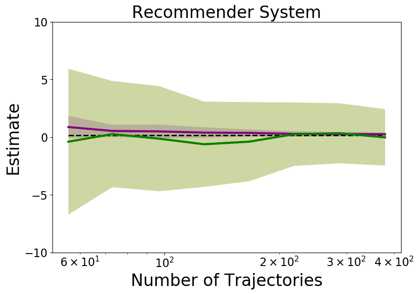
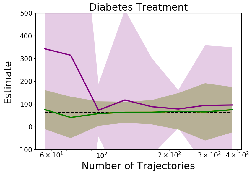
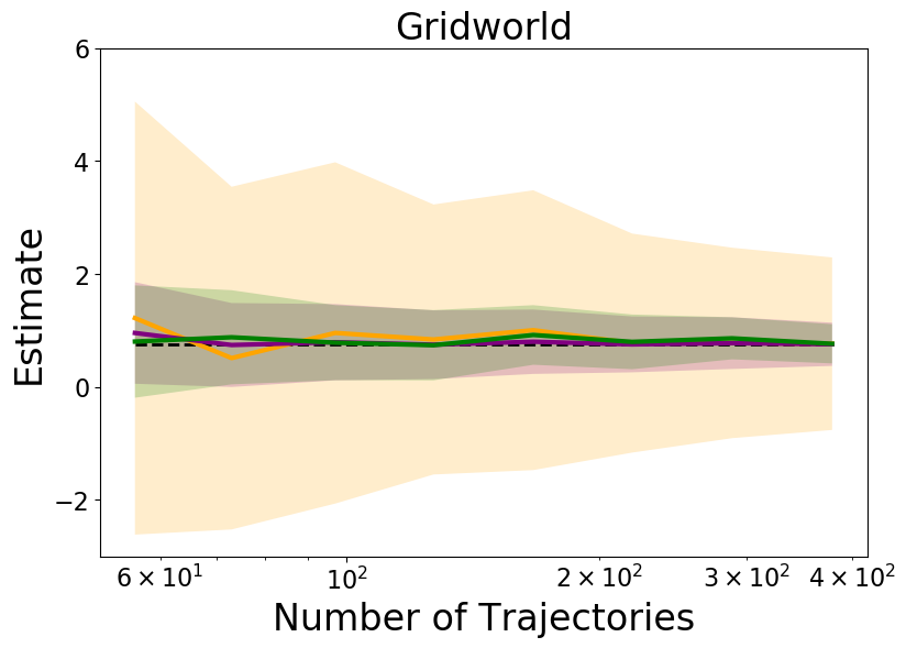
Figure 5: Comparison of different estimators on three domains. The estimate value for $\sigma^{2!!}$ was outside the limits of the y-axis for all the domains and hence is not visible. For the recommender system and the diabetes treatment domain, proposed estimators $\hat{\sigma}_{n}^{2}$, with and without coupled-decision importance sampling (CDIS), overlap. Results were averaged over 100 trials and the shaded regions correspond to one standard deviation.

References

- Anderson (1965) Anderson, R. 1965. Negative variance estimates. Technometrics 7(1): 75–76.
- Bastani (2014) Bastani, M. 2014. Model-free intelligent diabetes management using machine learning. M.S. Thesis, University of Alberta .
- Bellemare, Dabney, and Munos (2017) Bellemare, M. G.; Dabney, W.; and Munos, R. 2017. A distributional perspective on reinforcement learning. arXiv preprint arXiv:1707.06887 .
- Bottou et al. (2013) Bottou, L.; Peters, J.; Quiñonero-Candela, J.; Charles, D. X.; Chickering, D. M.; Portugaly, E.; Ray, D.; Simard, P.; and Snelson, E. 2013. Counterfactual reasoning and learning systems: The example of computational advertising. The Journal of Machine Learning Research 14(1): 3207–3260.
- Box (1953) Box, G. E. 1953. Non-normality and tests on variances. Biometrika 40(3/4): 318–335.
- Chernozhukov, Fernández-Val, and Melly (2013) Chernozhukov, V.; Fernández-Val, I.; and Melly, B. 2013. Inference on counterfactual distributions. Econometrica 81(6): 2205–2268.
- Dabney et al. (2017) Dabney, W.; Rowland, M.; Bellemare, M. G.; and Munos, R. 2017. Distributional reinforcement learning with quantile regression. arXiv preprint arXiv:1710.10044 .
- Di Castro, Tamar, and Mannor (2012) Di Castro, D.; Tamar, A.; and Mannor, S. 2012. Policy gradients with variance related risk criteria. arXiv preprint arXiv:1206.6404 .
- DiCiccio and Efron (1996) DiCiccio, T. J.; and Efron, B. 1996. Bootstrap confidence intervals. Statistical Science 189–212.
- DiNardo, Fortin, and Lemieux (1995) DiNardo, J.; Fortin, N. M.; and Lemieux, T. 1995. Labor market institutions and the distribution of wages, 1973-1992: A semiparametric approach. Technical report, National Bureau of Economic Research.
- Donald and Hsu (2014) Donald, S. G.; and Hsu, Y.-C. 2014. Estimation and inference for distribution functions and quantile functions in treatment effect models. Journal of Econometrics 178: 383–397.
- Efron and Tibshirani (1994) Efron, B.; and Tibshirani, R. J. 1994. An introduction to the Bootstrap. CRC press.
- García-Pérez (2006) García-Pérez, A. 2006. Chi-square tests under models close to the normal distribution. Metrika 63(3): 343–354.
- Guo, Thomas, and Brunskill (2017) Guo, Z.; Thomas, P. S.; and Brunskill, E. 2017. Using options and covariance testing for long horizon off-policy policy evaluation. In Advances in Neural Information Processing Systems, 2492–2501.
- Hanna, Stone, and Niekum (2017) Hanna, J. P.; Stone, P.; and Niekum, S. 2017. Bootstrapping with models: Confidence intervals for off-policy evaluation. In Proceedings of the 16th International Conference on Autonomous Agents and Multiagent Systems.
- Hoeffding (1994) Hoeffding, W. 1994. Probability inequalities for sums of bounded random variables. In The Collected Works of Wassily Hoeffding, 409–426. Springer.
- Hoover (2011) Hoover, K. D. 2011. Counterfactuals and causal structure. Oxford University Press Oxford.
- Horvitz and Thompson (1952) Horvitz, D. G.; and Thompson, D. J. 1952. A generalization of sampling without replacement from a finite universe. Journal of the American statistical Association 47(260): 663–685.
- Jaulin, Braems, and Walter (2002) Jaulin, L.; Braems, I.; and Walter, E. 2002. Interval methods for nonlinear identification and robust control. In Proceedings of the 41st IEEE Conference on Decision and Control, 2002., volume 4, 4676–4681. IEEE.
- Jiang and Li (2016) Jiang, N.; and Li, L. 2016. Doubly robust off-policy value evaluation for reinforcement learning. In International Conference on Machine Learning, 652–661. PMLR.
- Kostrikov and Nachum (2020) Kostrikov, I.; and Nachum, O. 2020. Statistical bootstrapping for uncertainty estimation in off-policy Evaluation. arXiv preprint arXiv:2007.13609 .
- Kuindersma, Grupen, and Barto (2013) Kuindersma, S. R.; Grupen, R. A.; and Barto, A. G. 2013. Variable risk control via stochastic optimization. The International Journal of Robotics Research 32(7): 806–825.
- Kuzborskij et al. (2020) Kuzborskij, I.; Vernade, C.; György, A.; and Szepesvári, C. 2020. Confident off-policy evaluation and selection through self-normalized importance weighting. arXiv preprint arXiv:2006.10460 .
- La and Ghavamzadeh (2013) La, P.; and Ghavamzadeh, M. 2013. Actor-critic algorithms for risk-sensitive MDPs. Advances in Neural Information Processing Systems 26: 252–260.
- Levene (1960) Levene, H. 1960. Robust tests for equality of variances. Contributions to probability and statistics In Olkin I, Ed.
- Lim and Loh (1996) Lim, T.-S.; and Loh, W.-Y. 1996. A comparison of tests of equality of variances. Computational Statistics & Data Analysis 22(3): 287–301.
- Liu et al. (2018) Liu, Q.; Li, L.; Tang, Z.; and Zhou, D. 2018. Breaking the curse of horizon: Infinite-horizon off-policy estimation. In Advances in Neural Information Processing Systems, 5356–5366.
- Man et al. (2014) Man, C. D.; Micheletto, F.; Lv, D.; Breton, M.; Kovatchev, B.; and Cobelli, C. 2014. The UVA/PADOVA type 1 diabetes simulator: New features. Journal of Diabetes Science and Technology 8(1): 26–34.
- Maurer and Pontil (2009) Maurer, A.; and Pontil, M. 2009. Empirical Bernstein bounds and sample variance penalization. arXiv preprint arXiv:0907.3740 .
- McHugh and Mielke (1968) McHugh, R. B.; and Mielke, P. W. 1968. Negative variance estimates and statistical dependence in nested sampling. Journal of the American Statistical Association 63(323): 1000–1003.
- Melly (2006) Melly, B. 2006. Estimation of counterfactual distributions using quantile regression .
- Metelli et al. (2020) Metelli, A. M.; Papini, M.; Montali, N.; and Restelli, M. 2020. Importance Sampling Techniques for Policy Optimization. Journal of Machine Learning Research 21(141): 1–75.
- Montgomery (2007) Montgomery, D. C. 2007. Introduction to statistical quality control. John Wiley & Sons.
- Nelder (1954) Nelder, J. 1954. The interpretation of negative components of variance. Biometrika 41(3/4): 544–548.
- Pan (1999) Pan, G. 1999. On a Levene type test for equality of two variances. Journal of Statistical Computation and Simulation 63(1): 59–71.
- Papini et al. (2019) Papini, M.; Metelli, A. M.; Lupo, L.; and Restelli, M. 2019. Optimistic Policy Optimization via Multiple Importance Sampling. In 36th International Conference on Machine Learning, volume 97, 4989–4999.
- Pearl (2009) Pearl, J. 2009. Causality. Cambridge University Press.
- Pearson (1931) Pearson, E. S. 1931. The analysis of variance in cases of non-normal variation. Biometrika 114–133.
- Pearson and Adyanthaya (1929) Pearson, E. S.; and Adyanthaya, N. 1929. The distribution of frequency constants in small samples from non-normal symmetrical and skew populations. Biometrika 21(1/4): 259–286.
- Precup (2000) Precup, D. 2000. Eligibility traces for off-policy policy evaluation. Computer Science Department Faculty Publication Series 80.
- Rowland et al. (2020) Rowland, M.; Harutyunyan, A.; Hasselt, H.; Borsa, D.; Schaul, T.; Munos, R.; and Dabney, W. 2020. Conditional importance sampling for off-policy learning. In International Conference on Artificial Intelligence and Statistics, 45–55. PMLR.
- Sakaguchi and Takano (2004) Sakaguchi, Y.; and Takano, M. 2004. Reliability of internal prediction/estimation and its application. I. Adaptive action selection reflecting reliability of value function. Neural Networks 17(7): 935–952.
- Sato, Kimura, and Kobayashi (2001) Sato, M.; Kimura, H.; and Kobayashi, S. 2001. TD algorithm for the variance of return and mean-variance reinforcement learning. Transactions of the Japanese Society for Artificial Intelligence 16(3): 353–362.
- Sbert, Havran, and Szirmay-Kalos (2018) Sbert, M.; Havran, V.; and Szirmay-Kalos, L. 2018. Multiple importance sampling revisited: breaking the bounds. EURASIP Journal on Advances in Signal Processing 2018(1): 15.
- Shao (1990) Shao, J. 1990. Bootstrap estimation of the asymptotic variances of statistical functionals. Annals of the Institute of Statistical Mathematics 42(4): 737–752.
- Sherstan et al. (2018) Sherstan, C.; Ashley, D. R.; Bennett, B.; Young, K.; White, A.; White, M.; and Sutton, R. S. 2018. Comparing direct and indirect temporal-difference methods for estimating the variance of the return. In UAI, 63–72.
- Sobel (1982) Sobel, M. J. 1982. The variance of discounted Markov decision processes. Journal of Applied Probability 19(4): 794–802.
- Stock and Watson (2015) Stock, J. H.; and Watson, M. W. 2015. Introduction to Econometrics.
- Subrahmaniam (1966) Subrahmaniam, K. 1966. Some contributions to the theory of non-normality-I (univariate case). Sankhyā: The Indian Journal of Statistics, Series A 389–406.
- Sutton and Barto (2018) Sutton, R. S.; and Barto, A. G. 2018. Reinforcement learning: An introduction. Cambridge, MA: MIT Press, 2 edition.
- Tabachnick and Fidell (2007) Tabachnick, B. G.; and Fidell, L. S. 2007. Experimental Designs Using ANOVA. Thomson/Brooks/Cole Belmont, CA.
- Tamar, Di Castro, and Mannor (2016) Tamar, A.; Di Castro, D.; and Mannor, S. 2016. Learning the variance of the reward-to-go. The Journal of Machine Learning Research 17(1): 361–396.
- Tamar and Mannor (2013) Tamar, A.; and Mannor, S. 2013. Variance adjusted actor critic algorithms. arXiv preprint arXiv:1310.3697 .
- Teevan et al. (2009) Teevan, J. B.; Dumais, S. T.; Liebling, D. J.; and Horvitz, E. J. 2009. Using variation in user interest to enhance the search experience. US Patent App. 12/163,561.
- Thomas and Brunskill (2016) Thomas, P.; and Brunskill, E. 2016. Data-efficient off-policy policy evaluation for reinforcement learning. In International Conference on Machine Learning, 2139–2148.
- Thomas, Theocharous, and Ghavamzadeh (2015) Thomas, P. S.; Theocharous, G.; and Ghavamzadeh, M. 2015. High-confidence off-policy evaluation. In Twenty-Ninth AAAI Conference on Artificial Intelligence.
- Wasserman (2006) Wasserman, L. 2006. All of nonparametric statistics. Springer Science & Business Media.
- White and White (2016) White, M.; and White, A. 2016. A greedy approach to adapting the trace parameter for temporal difference learning. arXiv preprint arXiv:1607.00446 .
- Xie (2019) Xie, J. 2019. Simglucose v0.2.1 (2018). URL https://github.com/jxx123/simglucose.
- Xie, Ma, and Wang (2019) Xie, T.; Ma, Y.; and Wang, Y.-X. 2019. Towards optimal off-policy evaluation for reinforcement learning with marginalized importance sampling. In Advances in Neural Information Processing Systems, 9668–9678.