Claimed detection of PH3 in the clouds of Venus is consistent with mesospheric SO₂

Abstract

The observation of a 266.94 GHz feature in the Venus spectrum has been attributed to PH3 in the Venus clouds, suggesting unexpected geological, chemical or even biological processes. Since both PH3 and SO2 are spectrally active near 266.94 GHz, the contribution to this line from SO2 must be determined before it can be attributed, in whole or part, to PH3. An undetected SO2 reference line, interpreted as an unexpectedly low SO2 abundance, suggested that the 266.94 GHz feature could be attributed primarily to PH3. However, the low SO2 and the inference that PH3 was in the cloud deck posed an apparent contradiction. Here we use a radiative transfer model to analyze the PH3 discovery, and explore the detectability of different vertical distributions of PH3 and SO2. We find that the 266.94 GHz line does not originate in the clouds, but above 80 km in the Venus mesosphere. This level of line formation is inconsistent with chemical modeling that assumes generation of PH3 in the Venus clouds. Given the extremely short chemical lifetime of PH3 in the Venus mesosphere, an implausibly high source flux would be needed to maintain the observed value of 20$\pm$10 ppb. We find that typical Venus SO2 vertical distributions and abundances fit the JCMT 266.94 GHz feature, and the resulting SO2 reference line at 267.54 GHz would have remained undetectable in the ALMA data due to line dilution. We conclude that nominal mesospheric SO2 is a more plausible explanation for the JCMT and ALMA data than PH3.

1 Introduction

Greaves et al. (2020a) recently attributed a 266.94 GHz (1.123 mm) line observed in the Venus spectrum to $\sim$20 ppb of phosphine (PH3) absorbing above 56 km altitude, in the upper clouds. In the strongly-oxidizing Venus atmosphere, PH3 formation is disfavored and its destruction is enhanced, leading Greaves et al. (2020a) to argue that its presence in the clouds points to unknown geological, chemical or even biological processes. The discovery team identified no viable abiotic production mechanism for PH3 in the Venus atmosphere (Greaves et al., 2020a; Bains et al., 2020), and so a biological origin was considered. PH3 has been proposed as a potential biosignature in terrestrial planet atmospheres (Sousa-Silva et al., 2020) due to its association with decaying organic matter (Glindemann et al., 2005), and significant—presumed biological—fluxes from marine environments on Earth (Zhu et al., 2007). However, the specific mode of biological production of PH3 remains uncertain and is still vigorously debated (Roels & Verstraete, 2001), with no known direct metabolic pathway (Roels et al., 2005).

The identification of PH3 in the Venus clouds was made using multiple observations of a single spectral feature at 266.94 GHz, where both PH3 (266.944 GHz) and SO2 (266.943 GHz) have absorption lines (Greaves et al., 2020a). After the initial detection using coadded spectra from the James Clark Maxwell Telescope (JCMT), which were taken over 5 nights between 2017 June 9–16, follow-up observations were made with the Atacama Large Millimeter Array (ALMA) on 2019 March 5. The latter dataset included simultaneous narrow-band (0.1171875 GHz) and wide-band (1.875 GHz) observations, centered on the Venus rest-frame PH3 frequency. The 266.94 GHz line, seen in the JCMT data at a S/N of 4.3 (Greaves et al. 2020a; although this detection significance has been subsequently called into question, Thompson 2020), was also detected in the ALMA narrowband and wideband datasets at higher significance than in the JCMT data (Greaves et al., 2020a), although a subsequent reanalysis of the ALMA data also suggests a less significant detection, with a correspondingly lower inferred abundance of PH3 (Greaves et al., 2020b). Assuming a uniform mixing ratio for the PH3, Greaves et al. (2020a) derive an abundance of 20 ppb from the JCMT observations, and calculate an emission weighting function peaked at 56 km. They therefore conclude that the PH3 absorption feature was sourced primarily from within the Venus clouds. However, as Greaves et al. (2020a) point out, with a FWHM of 4–5 km s^-1, this line could potentially contain contributions from both PH3 and SO2, as the SO2 line center is only +1.3 km s^-1 from the PH3 line center.

Consequently, the PH3 line identification is strongly dependent on accurately estimating and excluding a potentially-significant contribution from SO2, which, after the bulk atmospheric gases CO2 and N2, is the third most abundant gas in the Venus atmosphere. Greaves et al. (2020a) attempted to quantify the SO2 contribution to the observed 266.94 GHz feature by searching the ALMA wide-band observations for the nearby, stronger SO2 $J_{K_{a},K_{c}}=13_{3,11}\leftarrow 13_{2,12}$ 267.537 GHz line, but did not detect it (see their Figure 4a). Instead, they estimated a 10 ppb upper limit for SO2, based on potentially large spectral “ripples”, artifacts in the data induced by interferometric response to Venus as a bright, extended source. Greaves et al. (2020a) also noted that the $\leq 10$ ppb value was comparable to a 346.652 GHz ALMA Venus SO2 measurement of $16.5\pm 4.6$ ppb, which was taken in 2011 (Piccialli et al., 2017). However, the Piccialli et al. (2017) observation was sensitive to SO2 at 85 km altitude (Piccialli et al., 2017) in the Venus mesosphere (which extends from 65–120 km), and not to the middle/upper cloud deck (53–61 km). The $\leq 10$ ppb constraint derived from the non-detection implied a maximum 10% contribution from SO2 to the 266.94 GHz absorption band depth, and a shift in the observed line centroid of no more than 0.1 km s^-1. Greaves et al. (2020a) concluded that SO2 had been ruled out as a significant contaminant for the putative PH3 line. Conversely, they argued that the 266.94 GHz line could not be explained solely by SO2, because the corresponding reference lines would be significantly stronger than the $-0.0006$ l:c (line-to-continuum) ratio limit set by the spectral ripples, and yet the reference lines were not detected.

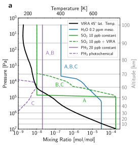
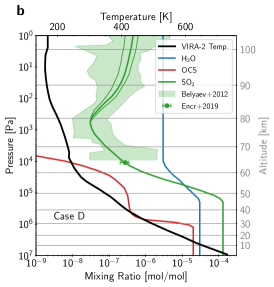
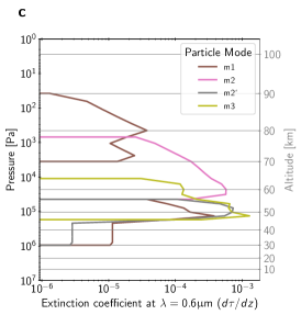
Figure 1: Atmospheric structures for Venus used in our spectral modeling cases. Panel a: Temperature and vertical profiles for Cases A–C, which use parameters assumed/derived by Greaves et al. (2020a). Temperature profile (black line) is for VIRA 45^∘ latitude (Seiff et al. 1985), and vertical profiles are shown for PH3 (solid, Cases A, B; dashed Case C), SO2 (green), and H2O (blue). Panel b: Temperature and vertical profiles for our Case D best fit to the JCMT 266.94 GHz line. The temperature profile (black line) is from VIRA-2 (Moroz & Zasova, 1997). The nominal gas mixing ratios for H2O (blue line) is based on VIRA values (von Zahn & Moroz, 1985) updated for the lower atmosphere (De Bergh et al., 2006) but have also been modified slightly as described in § 2. For OCS (red line), the profile is constructed based on recent measurements by Krasnopolsky (2010) and Arney et al. (2014), and by the surface abundance in the lower atmosphere model by Krasnopolsky (2013). For SO2 (green line), we fit the 266.94 GHz line guided by the vertical profile of Belyaev et al. (2012) in the mesosphere and upper cloud, and consistent with a suite of SOIR and SPICAV UV SO2 measurements taken from 2007–2008 (green shaded region). This profile passes through the cloud-top SO2 measurement (200–350 ppb) obtained by Encrenaz et al. (2019) in July 2017 (green data point), one month after the Greaves et al. (2020a) JCMT observations. We use 130 ppm in the lower atmosphere (Marcq et al., 2008) and generated a profile between the lower atmosphere and cloud tops. Panel c: optical depth extinction profiles (optical depth per meter at a wavelength of 0.6 $\upmu$m) for the Venus cloud particle modes: m1 (haze), m2, m2’, and m3 (Crisp, 1986). The clouds are defined via optical depth considerations to span approximately 48–70 km ($3\times 10^{3}$–$1.3\times 10^{5}$ Pa).

Because the non-detection of SO2 by Greaves et al. (2020a) supports a corresponding low inferred abundance, and a low contamination fraction for the 266.94 GHz line, it is the key piece of evidence supporting the PH3 line identification at 266.94 GHz— and so it warrants closer scrutiny. There is an apparent contradiction between the inferred altitudes that the PH3 feature probed, and the SO2 abundance constraint. If the putative PH3 (266.94 GHz) absorption is sensitive to altitudes near 56 km, and thus probes the Venus middle and upper cloud, then the 267.94 GHz SO2 reference line should also originate from this altitude range, since it has similar line strength and amount of underlying continuum absorption. Data and modeling estimates place the SO2 abundance near 1–5 ppm at 60 km in the upper cloud, which should increase with depth to match the higher $\sim$130 ppm measured below the cloud deck (Zasova et al., 1993; Krasnopolsky, 2012; Zhang et al., 2012; Belyaev et al., 2012; Marcq et al., 2008; Arney et al., 2014; Encrenaz et al., 2019). Previous measurements therefore suggest that the inferred disk-averaged $<10$ ppb of SO2 is anomalously low, especially if the observations probe within the clouds. Assuming similar spatial distribution of the two gases, for an inferred SO2 abundance at 56 km of 10ppm, and the 10 ppb PH3 abundance of Greaves et al. (2020a), the SO2 contribution to the observed line would exceed that from PH3 by two orders of magnitude (Krasnopolsky, 2020).

If the observations were instead sensitive to the mesospheric levels above the clouds, as is the case for higher frequency ALMA observations (Sandor et al., 2010; Encrenaz et al., 2015), then the inferred Venus SO2 abundance would be closer to, but still lower than previously measured levels (Sandor et al., 2010; Encrenaz et al., 2015; Piccialli et al., 2017; Vandaele et al., 2017). While the abundance of SO2 above the clouds is known to vary significantly over time (Esposito et al., 1988; Encrenaz et al., 2012, 2019) with a minimum observed around 10-100 ppb at $\sim$80 km, the abundances in the mesosphere have been measured to be in the range 10 ppb to 10 ppm (Krasnopolsky, 2010; Belyaev et al., 2012; Vandaele et al., 2017). A planet-wide decrease from a higher cloud-top SO2 abundance in 2006 to a low in 2014 of 30 ppb was also observed, but more recent observations from 2016 through September 2018, which span the Greaves et al. (2020a) JCMT observation, show a strong increase to typical cloud-top values of several hundred ppb of SO2 (Encrenaz et al., 2019).

While line absorption occurring predominantly within the mesosphere would make the non-detection and inferred low abundance of SO2 more plausible, it would also suggest that the line attributed to PH3 was formed at mesospheric levels. Consequently, the 266.94 GHz line would not be sensitive to, and so not able to confirm, the presence of PH3 in the Venus clouds—potentially weakening support for a biological origin. The presence of 20 ppb of mesospheric PH3 would require an extremely large source flux due to photolysis and reactions with radical species, including Cl and H, that result in a sub-second lifetime for PH3 in the Venus mesosphere (Bains et al., 2020, their Fig. 2). Indeed, the vertical distribution predicted using photochemical-kinetics studies with a cloud source of PH3 indicates a sharply reduced mesospheric abundance of PH3 ($<0.001$ ppb) alongside significant ($>100$ ppb below 95 km) SO2 (Greaves et al. 2020a, extended data figure 9; Bains et al. 2020).

To explore the potential contradictions posed by the Greaves et al. (2020a) PH3 observations, and to verify the source region for the 266.94 GHz absorption, here we use a radiative transfer model of the Venus atmosphere to simulate the impact on the Venus millimeter-wavelength spectrum of different abundances and vertical distributions of PH3 and SO2, including those proposed by Greaves et al. (2020a) and Bains et al. (2020).

2 Methods

To generate synthetic millimeter-wavelength spectra of Venus, we use SMART (Spectral Mapping Atmospheric Radiative Transfer), a 1D line-by-line, multi-stream, fully multiple-scattering radiative transfer model (Meadows & Crisp, 1996; Crisp, 1997). SMART has been validated against observations of Solar System planets, with heritage modeling the Venus atmosphere (Meadows & Crisp, 1996; Arney et al., 2014; Robinson & Crisp, 2018).

Our spectral simulations consist of Cases A–C, for which we generate spectra based on the mixing ratios and vertical profiles used and derived by Greaves et al. (2020a), and our best fit model, Case D, which does not contain PH3 and uses constraints from additional Venus observations (Figure 1). Cases A–C include CO2, SO2, H2O, and PH3 and use the VIRA 45^∘ latitude temperature profile (Seiff et al., 1985). To match the H2O estimate of Greaves et al. (2020a), we use the De Bergh et al. (2006) H2O profile but reduced to 0.2 ppm above 68 km. For SO2, we use the De Bergh et al. (2006) compilation below 100 km for cases B and C, but reduced to 10 ppb above 70 km, and for case A we maintain 10 ppb down through the cloud deck to 53 km. For PH3, we use a uniformly mixed 20 ppb profile for cases A and B, and the photochemical profile from Greaves et al. (2020a) (their figure ED7) for case C.

For our best-fit scenario, Case D, we do not include PH3 and use the De Bergh et al. (2006) update to the VIRA below 100 km and more recent observations where available. We use the VIRA-2 temperature profile (Moroz & Zasova, 1997). For H2O, we use 30 ppm below the cloud deck (De Bergh et al., 2006, and references therein), and we assume 3 ppm above the cloud deck (Krasnopolsky et al., 2013; Cottini et al., 2015; Piccialli et al., 2017). For SO2, we use 130 ppm below the cloud deck (Gelman et al., 1979; Bezard et al., 1993; De Bergh et al., 2006; Marcq et al., 2008; Arney et al., 2014), decreasing with increasing altitude to the July 2017 observation of $\sim$275 ppb at 64 km (Encrenaz et al., 2019), which was measured within a month of the Greaves et al. (2020a) JCMT data. In the mesosphere, we fit the SO2 profile to the observed feature at 266.94 GHz guided by the vertical profile fit to 2007–2008 data from Belyaev et al. (2012), which is consistent with the cloud-top SO2 abundance observed in July, 2017 (see Encrenaz et al., 2019). Long-term monitoring has shown that 2007–2008 and 2017–2018 were similar maximum periods of global mesospheric SO2 abundance (Encrenaz et al., 2019), although short-term temporal variability within these secular changes can be orders of magnitude (Belyaev et al., 2017). We prescribe the OCS profile guided by recent measurements (Krasnopolsky, 2010; Arney et al., 2014) and models (Zhang et al., 2012; Krasnopolsky, 2012, 2013; Lincowski et al., 2018). We adopt the same aerosol properties, modes, and optical depth profiles as Arney et al. (2014), which originate from Crisp (1986). Temperature and gas profiles, and aerosol optical depths, are shown in Figure 1.

Absorption cross-sections associated with vibrational-rotational transitions are calculated using a line-by-line model, LBLABC (see Meadows & Crisp, 1996; Crisp, 1997, for details), with the HITRAN2016 line database (Gordon et al., 2017) for all gases except CO2, which is calculated from the extensive Ames line database (Huang et al., 2017). Because these line lists assume terrestrial isotopic abundance, we use the methods described in Lincowski et al. (2019) to adjust the line list isotopologue abundances for H2O to 200 times the D/H abundance compared to Earth, the standard value used in the literature for the Venus mesosphere (Encrenaz et al., 2015). Collision-induced absorption data is used for CO2-CO2 (Gruszka & Borysow, 1997).

Data on the foreign broadening of gases by CO2 is not well-characterized, compared to broadening by air, but is more appropriate for Venus simulations. To reproduce the results of Greaves et al. (2020a), we use their foreign broadening parameter for PH3 of 0.186 cm^-1 atm^-1, which they used to estimate PH3 as 20$\pm 10$ ppb in the JCMT data. Because their broadening treatment for gases other than PH3 is not specified, we use the default HITRAN air broadening for cases A–C. To fit the 266.94 GHz detection feature with SO2 in case D, we employ data for broadening by CO2, as available. For SO2 and OCS, we use data for broadening by CO2 available in HITRAN (Wilzewski et al., 2016; Gordon et al., 2017). Although the SO2 broadening data are derived from a single line experiment (Chandra & Chandra, 1963), the parameters in the frequencies of interest are consistent with recent laboratory results by Bellotti & Steffes (2015). The broadening values for our SO2 lines of interest are approximately 1.8–2.0$\times$ air broadening (i.e. $\gamma_{\ce{CO2}}\simeq 0.17-0.19$ cm^-1 atm^-1). For HDO, we multiply the HITRAN air foreign broadening parameters by 2.4, which is consistent with this frequency range (Sagawa et al., 2009).

To better visualize individual line signal and compare to the published data, we processed our flux spectra to normalize the continuum. Because we are processing noiseless model results, we mask spectral intervals for individual lines and linearly interpolate the continuum across the interval. The line:continuum (l:c) spectra were determined by dividing the original model spectrum by the continuum and subtracting one.

As an additional validation of our radiative transfer model and fit to the Greaves et al. (2020a) JCMT data, we applied our model to simulate the line shape and peak intensity of the 346.65 GHz late-2011 observation of Encrenaz et al. (2015), using their SO2 profile of 10 ppb from 86–100 km, and obtained an excellent fit to the data (see Fig. 2).

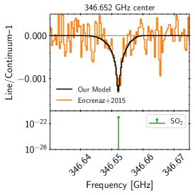
Figure 2: We demonstrate the validity of our model by fitting the 346.652 GHz SO2 line observed by Encrenaz et al. (2015, Fig. 19) in 2011 using their best-fit profile of no SO2 from 70–85 km and 10 ppb above 85 km, with all other modeling parameters specified as for our Case D (but also including CO from the De Bergh et al. (2006) compilation). SO2 absorption line strength in the bottom panel is given in units of cm^-1/(molecule cm^-2). This comparison shows our model and associated parameters are consistent with previous sub-mm observations of SO2.

3 Results

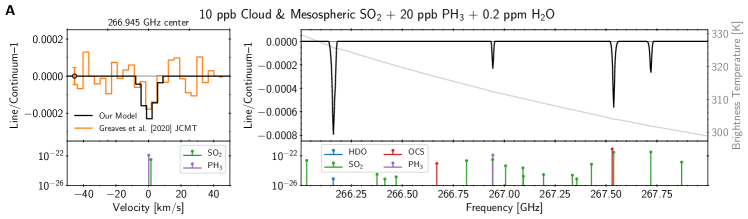
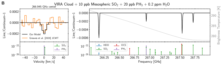
Figure 3: Venus spectral simulations for different PH3 and SO2 abundances and vertical profiles, including brightness temperature spectra (grey lines) to show the continuum source, and absorption line strengths (lower panels in each case) in units of cm^-1/(molecule cm^-2). For each case, the left hand panel shows the corresponding fit to the 266.94 GHz line, the right panel shows the 266–268 GHz spectrum, including the SO2 reference line at 267.54 GHz. Case A: modified VIRA temperature and gas profiles with uniformly mixed 20 ppb PH3 and 10 ppb SO2 down through the cloud deck (c.f. Figure 1 Panel a). Case B: Case A but with the VIRA SO2 profile in the cloud deck up to 70 km instead of evenly mixed at 10 ppb. Case C: VIRA and SO2 profile as in Case B, but using the photochemically self-consistent profile for PH3 from Greaves et al. (2020a) (ED Fig. 9). Case D: VIRA-2 temperature profile, no PH3, and using a vertically-resolved SO2 profile derived from a suite of spacecraft and ground-based measurements, with a mesospheric profile that increases from 30 ppb at 78 km to 400$\pm$150 ppb at 100 km (see Figure 1, panel b). Cases A and B demonstrate similar fits for PH3 to the the 266.94 GHz line as in Greaves et al. (2020a), and show lack of sensitivity to the vertical distribution of SO2 in the clouds. Case C demonstrates that the PH3 profile generated assuming a source in the Venus clouds is inconsistent with the observed 266.94 GHz line. Case D shows that we can fit the detection feature with no PH3 but with a typical Venus SO2 abundance, although this produces SO2 reference line features that are over 10 times stronger than the other cases.

To explore the spectral impacts of different abundances and vertical profiles for PH3 and SO2, we simulated spectra of Venus from 266 to 268 GHz. This spectral range includes the HDO, PH3 and SO2 line positions discussed in Greaves et al. (2020a), as well as OCS, which includes a transition at 267.530 GHz. We simulated spectra for cases with the abundances determined by Greaves et al. (2020a) and vertical profiles determined by previous measurements of the Venus atmosphere (Figure 1). Line-to-continuum (l:c) spectra generated at 0.0001 cm^-1 (3 MHz) resolution are shown in Figure 3, along with the emission brightness temperature in grey. The brightness temperatures demonstrate the effective altitude of continuum emission, and are directly correlated with SO2 abundance in the cloud deck between 54–57 km, depending on the case. Lower cloud SO2 abundance (10 ppb evenly-mixed) yields higher continuum emission from deeper in the atmosphere.

3.1 Simulated Spectra

For our Case A spectral simulation (Figure 3A) we assumed updated VIRA-derived profile (our Figure 1, see von Zahn & Moroz 1985; De Bergh et al. 2006) for all constituents except SO2 and PH3. Following Greaves et al. (2020a), we assumed an evenly mixed abundance of 20 ppb PH3 and 10 ppb SO2 above 52 km altitude (near the base of the Venus cloud deck; green and purple dotted lines in Figure 1a). We also assumed their foreign broadening parameter for PH3 of 0.186 cm^-1 atm^-1. Our model produces a comparable fit to Greaves et al. (2020a) for the 266.94 GHz line (c.f. their Figure 1). Additionally, with the evenly-mixed 10 ppb of SO2, we also confirm that the 267.54 GHz SO2 line is below the spectral-ripple-inferred maximum limit on the l:c ratio ($-0.0006$).

In our Case B simulation (Figure 3B), instead of assuming the low 10 ppb SO2 down through the cloud deck, we used the VIRA-derived profile such that the SO2 abundance increased with cloud depth (green dashed line in Figure 1b). At the 56 km level, the SO2 abundance is now closer to 20 ppm. The increased SO2 opacity raises the emission layer to cooler levels of the atmosphere, as shown in the the brightness temperature difference between Cases A and B. This produces a small change in the SO2 continuum, which results in only marginal differences in the intensities of the 266.94 GHz PH3 line and the 267.54 GHz SO2 line, and the latter is still consistent with the maximum limit in sensitivity due to spectral ripple. Thus the observed line intensities are largely insensitive to SO2 abundance within the clouds.

In our Case C simulation (Figure 3C), we again used 10 ppb SO2 in the mesosphere, increasing through the cloud deck (green dashed line in Figure 1a). However, instead of PH3 evenly mixed throughout the atmosphere (as in Cases A and B), we used the photochemical profile for PH3 used to interpret the 266.94 GHz detection, as provided in Greaves et al. (2020a, their ED Figure 9), and Greaves et al. (2020a, reproduced as the purple dashed line in our Figure 1a). This distribution is derived from the assumption that PH3 production is concentrated within the cloud deck with abundance dropping rapidly in the upper cloud deck and mesosphere, and more slowly towards the surface. The small absorption line present here at 266.94 GHz is due to SO2—no PH3 absorption is visible in this spectral simulation. This indicates that the line core observation is not sensitive to PH3 in the cloud, and demonstrates that the assumed profile in the Greaves et al. (2020a) and Bains et al. (2020) photochemical simulations are inconsistent with the JCMT observations.

In our Case D simulation (Figure 3D), we removed PH3 from our atmosphere and fit the JCMT detection feature at 266.94 GHz using SO2 alone. As described in §2, we used parameters for HDO, SO2, and OCS foreign broadening by CO2. We guided the mesospheric data fit for SO2 using Venus Express UV/IR occultation data from Belyaev et al. (2012). This profile is consistent with cloud-top SO2 abundances measured by Encrenaz et al. (2019) within a month of the Greaves et al. (2020a) JCMT observations. Our best-fit SO2 profiles, fitting the observed line (black) and $\pm$1-$\sigma$ about the line (grey) are shown in Figure 1b (green curves), with SO2 increasing from 30 ppb at 78 km to 400$\pm$150 ppb at 100 km. These abundance profiles are well within the range of measurements compiled in Belyaev et al. (2012) and Vandaele et al. (2017). This simulation provides an excellent fit to the JCMT detection line without PH3, and predicts a pair of SO2 reference lines that have l:c ratios a factor of $\sim$10 higher than those seen in the previous simulations.

3.2 Spectral Line Sensitivity

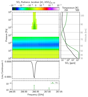
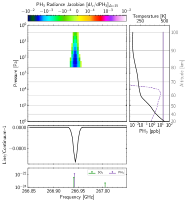
Figure 4: Radiance mixing ratio Jacobians ($dI_{\nu}/dr_{\text{mix}}$) as a function of layer pressure for the radiance streams at 21 degrees zenith angle, for the 266.94 GHz feature for SO2 (left) or PH3 (right). Absorption line strengths (lower panels in each case) are given in units of cm^-1/(molecule cm^-2). The continuum originates from SO2 at $\sim 6\times 10^{4}$ Pa ($\sim$54 km, within the cloud deck), while the line cores for either species do not originate in the clouds (48-70 km) but at over 400 Pa (over 80 km) in the mesosphere. In the right panels in both plots, the temperature structure is given as a black line, while the colored lines denote SO2 (green) or PH3 (purple) mixing ratios. On the right, the evenly-mixed 20 ppb PH3 profile is shown with a solid line and the photochemical PH3 profile is shown with a dashed line.

To confirm the altitudinal sensitivity of the 266.94 GHz line for key PH3 and SO2 vertical profiles, we calculated radiance Jacobians, i.e. the increase in top-of-atmosphere radiance as a function of perturbations to the abundances for SO2 and PH3 at each layer of our model atmosphere (Figure 4). The outgoing radiance will be most sensitive to regions of the atmosphere that contribute most to the spectral feature. The Jacobians show that the observed line cores for both gases originate from atmospheric pressures only as deep as $\sim$400 Pa, corresponding to altitudes of $\geq$80 km, in the mesosphere. This absorption feature cannot be generated at levels within the cloud deck, where the background continuum emission originates. It must be generated well above this layer, where the absorbing gas is cooler and therefore absorbs more efficiently than it emits. The narrow width of the absorption line also suggests that it was formed at pressures substantially less than those of the cloud top (70 km, $\sim$3000 Pa).

3.3 ALMA Line Dilution

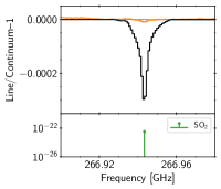
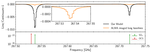
Figure 5: Modeled line dilution for the ALMA observations: disk-averaged line/continuum ratios for our nominal Case D atmosphere model containing SO2 uniformly distributed over the Venus disk, at 0.00003 cm^-1 (1 MHz) resolution (black lines), for the detection frequency (left panel) and reference lines frequencies (right panel). Absorption line strengths (lower panels) are given in units of cm^-1/(molecule cm^-2). The orange lines show the same spectral model as imaged using the ALMA antenna configuration of the Greaves et al. (2020a) observations. The inset shows the suppression of the 267.54 GHz reference line to an l:c of close to $-0.0003$. The line intensity is significantly diluted, and is consistent with the non-detection of these SO2 absorption lines in the wideband data.

While the non-detection of prominent SO2 spectral features in the ALMA wideband data could indicate a low abundance, as argued by Greaves et al. (2020a), the estimation of this abundance was done without correcting for line dilution as a result of the ALMA observing geometry (Greaves et al., 2020a). Significant line dilution is likely, especially considering the global distribution of SO2 in the Venus atmosphere, and the exclusion of the short baseline ALMA measurements. Greaves et al. (2020a) estimated line dilution (filtering losses) of 60–92% depending on position on the disk. To determine the disk-averaged line dilution for the SO2 reference line search, we simulated observations of Venus using the ALMA configuration of Greaves et al. (2020a) by imposing an appropriate resolution spectrum (0.00003 cm^-1, 1 MHz) of our Case D atmospheric model over a limb-darkened disk model. The Fourier Transform of this model was re-sampled to match the ALMA configuration and re-imaged using the imaging routines of Greaves et al. (2020a), as provided in their Supplementary Software 3. As shown in Figure 5, line dilutions on the order of 95% at the line core are observed for the full disk. We observe similar dilutions when the spectrum is only imposed on one hemisphere ($\sim$8 arcsecond extent at the time of observation). This line dilution suggests that the SO2 reference features produced by our best fit SO2 distribution (Case D) would be heavily suppressed by line dilution in the ALMA data, which would cause them to mimic smaller features below the ripple detection limit of $-0.0006$.

4 Discussion

The claim that PH3 has been detected in the Venus clouds is currently supported by observations of a single absorption line at a frequency that also coincides with absorption from SO2, a known and relatively common Venus gas, and based on an emission weighting function that peaks at 56 km (Greaves et al., 2020a). However, our radiative transfer analysis indicates that the line at 266.94 GHz does not measure absorption within the Venus clouds. Our explicit calculation of radiance Jacobians confirms the assessment that both 266.94 GHz PH3 and SO2 line core absorption would be produced well above the Venus cloud deck at altitudes exceeding 80 km. Arguments for a mesospheric origin for the 266.94 GHz line core, based on the observed narrow width of the line, are also provided in a recent commentary by Villanueva et al. (2020). This mesospheric contribution is inconsistent with a vertical abundance profile that concentrates PH3 in the middle and upper clouds, as used by Greaves et al. (2020a) and Bains et al. (2020) to interpret their discovery. Our spectral simulation using this photochemical PH3 profile also shows that it is not consistent with the strength of the observed 266.94 GHz line. However, the presence of PH3 in the Venus clouds is not conclusively ruled out either, a point also made by Greaves et al. (2020b), because the Greaves et al. (2020a) observations are not sensitive to absorption at cloud deck altitudes, and so can neither exclude, nor confirm, the presence of PH3 in the Venus clouds.

Given that we have shown that the observed 266.94 GHz line predominantly originates high in the mesosphere, attributing it to PH3 is less chemically plausible than SO2. At these higher altitudes ($>$80 km) PH3 would be destroyed rapidly, while SO2 is photochemically regenerated (Sandor et al., 2010; Belyaev et al., 2012; Zhang et al., 2012). Between 82 km and 96 km (70–300 Pa, where the line core absorption originates, Fig. 4) PH3 has a sub-second lifetime, due to the destruction by Cl and H radicals and UV photolysis (Bains et al., 2020). To balance this rapid destruction rate and maintain a mesospheric concentration of 20 ppb, an extremely large flux of PH3 is required, potentially as large as $3.7\times 10^{15}$ molecules cm^-2 s^-1. For comparison, this production rate is about $\sim$100 times the flux of O2 produced by Earth’s global photosynthetic biosphere (Field et al., 1998), the dominant metabolism on our planet. Greaves et al. (2020a), assuming the 266.94 GHz absorption was from PH3 in the clouds, calculated a significantly smaller production rate of $10^{7}$ molecules cm^-2 s^-1, due to the lower destruction rate within the clouds. However, the assumption of this in-cloud production rate results in a PH3 mixing ratio that effectively falls to zero at $>$80 km altitude (Greaves et al., 2020a, Fig. 5b), which is inconsistent with our analysis that the observed line is sourced in the mesosphere. Although a recent reanalysis of the ALMA data by Greaves et al. (2020b) has greatly reduced the significance of the 266.94 GHz line detection, their assignment of 1 ppb of PH3 in the mesosphere would still require a production rate significantly higher than the Earth’s photosynthetic biosphere, and the larger 20 ppb PH3 value inferred from the JCMT data still stands.

These challenges to mesospheric production rate are not relevant if the observed 266.94 GHz line is instead attributed to SO2, which is known to increase in abundance with altitude in the mesosphere (Belyaev et al., 2012; Mills et al., 2018). A combination of infrared observations that probe the upper cloud and lower mesosphere, and UV occultation measurements that probe the upper mesosphere, has been used to map the vertical distribution of mesospheric SO2 (Belyaev et al., 2012, 2017). This distribution drops from the cloud tops to a minimum just below 80 km, but increases substantially from 80–100 km to typically several hundred ppb (Belyaev et al., 2012; Vandaele et al., 2017).

Assuming that the Venus atmosphere does not contain PH3, we find that a realistic vertical profile for SO2 fits the JCMT 266.94 GHz detection. Because the JCMT observations were single dish, any SO2 contribution to the 266.94 GHz line would not have been suppressed, as was the case for the ALMA data, and so should be sensitive to the true mesospheric SO2 abundance. We used a mesospheric SO2 profile that is based on the profile observed in 2007–2008 by Belyaev et al. (2012), which is likely a good fit to similar higher values seen in 2016–2018, a time span that includes the Greaves et al. (2020a) JCMT observation. This profile is also consistent with cloud top values of 200–350 ppb observed in the mid-infrared within a month of the Greaves et al. (2020a) JCMT observations (Encrenaz et al., 2019). The Encrenaz et al. (2019) observations support the validity of our SO2 vertical profile, and suggest that the Venus mesosphere was unlikely to be experiencing a period of anomalously low SO2 abundance at the time of the JCMT observations. Using this vertical abundance profile and a CO2-broadened SO2 line profile, we can fit the width and shape of the 266.94 GHz line using SO2 alone, without needing an additional PH3 component. The SO2 is also a better fit to the line centroid than the PH3 (cf. Fig. 3 A/B, D). This excellent fit counters the argument of Greaves et al. (2020b) that SO2 alone would be too narrow to fit the observed line. Greaves et al. (2020b) also recently argued that the SO2 abundance required to fit the JCMT 266.94 GHz line (evenly-mixed 150 ppb for their fit, and 100 ppb for Villanueva et al. 2020) is unrealistically large, given previous mm-wave observations, which have returned lower values for mesospheric SO2 (Sandor et al., 2010; Encrenaz et al., 2015). However, mm-wave observations do not have as long, or as well sampled, a baseline as dedicated Venus spacecraft observations of the mesosphere (Belyaev et al., 2012, 2017; Vandaele et al., 2017), and mesospheric SO2 abundance has been observed to vary by an order of magnitude on daily to yearly timescales, with values at 90–95 km altitude between 10 to 300 ppb. There is also evidence for longer-term secular changes in mesospheric and cloud-top SO2 abundances, with maxima in 2007–2008 and 2016–2018, and a minimum in 2012–2014 (Belyaev et al., 2017; Encrenaz et al., 2019). We note that the model that we used to fit the JCMT 266.94 GHz line assuming a higher abundance of SO2 also produced an accurate fit to the lower abundance observation of Encrenaz et al. (2015) (see our Fig. 2), which was observed near an SO2 minimum.

We also find that strong ALMA line dilution allows the vertical abundance profile of SO2 that fits the JCMT 266.94 GHz observations to still be consistent with the non-detection of the SO2 ALMA reference lines—which are likely poor indicators of the impact of SO2 on the JCMT observations. Spectral simulations using our Case D SO2 vertical distribution predict SO2 lines at 267.54 and 267.72 GHz with l:c ratios that are close to a factor of 10 larger than the nominal ALMA non-detection limit of $-0.0006$ given by Greaves et al. (2020a). This apparent contradiction can be reconciled by the lack of line-dilution in the JCMT observation of the 266.94 GHz line, as the single-dish integrates flux over all scales, while the telescope configuration and the removal of measurements from the $\leq 33$ m ALMA baselines would have likely resulted in at least 90–95% line dilution (factor of 10–20 suppression) for spatially-uniform SO2 gas. Therefore, taking the sensitivity of the two telescopes into account, our JCMT fit does not need to be adjusted, but our modeled SO2 l:c ratios should be divided by at least $\sim$20, if the SO2 is uniform across the disk, to approximate the ALMA detection for that set of baseline configurations. In doing so, our predicted SO2 reference line values fall below the “10 ppb” ($-0.0006$) detection threshold (see Figure 5 inset). Consequently, the SO2-only model with up to several hundred ppb of SO2 in the mesosphere can fit the JCMT data, and still be consistent with the non-detection of SO2 in the ALMA wide-band data. Moreover, this strong line dilution, with the corresponding loss of sensitivity to even high levels of SO2, suggests that the ALMA wide-band SO2 reference observations were likely poor indicators that SO2 was low enough to be ruled out as a significant source of the JCMT 266.94 GHz line—thereby significantly weakening the argument that this line was instead due primarily to PH3.

In addition to explaining the JCMT single-dish detection of the 266.94 GHz line, and the suppression of the SO2 reference lines in the ALMA data, our SO2-only hypothesis would also predict that the 266.94 GHz ALMA line would be, like the SO2 reference lines, strongly suppressed by line dilution and potentially non-detectable. While this was not the case in the original Greaves et al. (2020a) paper, this is now consistent with recent significant challenges to the detection confidence of the 266.94 GHz ALMA line. These include reanalyses of the Greaves et al. (2020a) narrowband ALMA discovery data by both Snellen et al. (2020) and Villanueva et al. (2020) who concluded that the feature attributed to PH3 could not be detected with statistical significance. Our own further analysis of the Greaves et al. (2020a) ALMA data, including testing the robustness of the detection at 266.94 GHz, comes to a similar conclusion, and is presented in Akins et al. (accepted). Additionally, a recent reanalysis of high-resolution, S/N$\sim$1000 Venus observations taken in 2015 was used to search for a PH3 transition near 10.47 $\upmu$m, but it was not detected, setting a stringent upper limit of 5 ppb above the Venus clouds (Encrenaz et al., 2020). Finally, the recent Greaves et al. (2020b) communication analyzing a reprocessing of the ALMA data suggests that the 266.94 GHz feature in the narrow-band whole-planet ALMA data is now significantly reduced in detection significance from the original discovery paper (4.8-$\sigma$ vs 13.3-$\sigma$), with an l:c of $-2\times 10^{-5}$, consistent with 1 ppb of PH3. However, this much-reduced 266.94 GHz feature would also be consistent with line-diluted SO2, which in our model would have l:c of $-1$ to $-2\times 10^{-5}$ at this frequency, for line dilution in the range 95–97%—which is likely well within the range of potential line dilution (Akins et al., accepted).

Although the SO2 hypothesis self-consistently explains our current understanding of the detection and non-detections in the JCMT and ALMA data, additional analyses and observations will be needed to more definitively discriminate between PH3 and SO2 as the source of the 266.94 GHz JCMT line. Re-observing Venus at 266.94 GHz will likely still be needed to independently confirm the discovery observation, and detection of an additional PH3 absorption feature would provide a much stronger case for its presence in the Venus atmosphere. Future observations to confirm the PH3 $J=1\leftarrow 0$ line detection should incorporate single dish measurements, which would not suffer from line dilution, or observations including the Atacama Compact Array (which includes shorter baseline measurements than the primary ALMA array). Because the SO2 abundance is critical to the PH3 identification for the ALMA data, we recommend that future attempts to confirm the ALMA PH3 observations should also obtain near-simultaneous SO2 measurements. The narrowband correlator configuration can be tuned to 266.94 GHz and to the frequencies of two nearby, stronger SO2 lines (near 267.54 and 267.72 GHz). To mitigate the spectral ripple features that compromised measurement of the line intensities (Greaves et al., 2020a), these observations should occur when the apparent angular diameter of Venus is smaller and therefore less resolved by the ALMA antennas.

Ultimately, the claimed detection of PH3 in the atmosphere of Venus has underscored the necessity of identifying and assessing the context of the environment within which we find potential biosignatures. The identification of the 266.94 GHz line as due to PH3, and its plausibility as a potential biosignature, is inextricably intertwined with the physical and chemical environment of the Venus cloud and above-cloud atmosphere. This initial, controversial detection has highlighted just how much we still need to understand about our sister planet, and how important that knowledge is in interpreting this discovery. If the 266.94 GHz line is confirmed, and conclusively attributed to PH3, its presence in the mesosphere would require additional observations to understand potential sources and sinks, and the attendant (and as yet unknown) phosphorous chemistry that enables its persistence at these high altitudes. Moreover, if PH3 is being generated abiotically, especially at these high altitudes, this would have negative implications for the robustness of PH3 and other reduced gases to serve as biosignatures in oxidizing terrestrial atmospheres. Regardless of the outcome, additional targeted observations will reveal processes on a terrestrial planet that informs our understanding of our own world, and potentially a large number of exoplanets that may share a similar evolutionary path and current environment.

5 Conclusions

We simulated millimeter-wavelength Venus spectra to explore the vertical distribution and detectability of PH3 and SO2 in the Venus atmosphere. We find that the observations of the 266.94 GHz absorption line are insensitive to the abundance of PH3 and SO2 within the cloud deck. Instead, the observed absorption at this wavelength originates from the mesosphere at altitudes above 80 km. At these altitudes, PH3 would be rapidly destroyed, such that $20\pm 10$ ppb of PH3 would require a flux of PH3 to the Venus mesosphere that is $\sim$100 times higher than the global production rate of photosynthetically-generated O2 on Earth. Because PH3 and SO2 both absorb within the width of the line detected at 266.94 GHz, we emphasize that the identification of this absorption line as due to PH3 in both the ALMA and JCMT data relies heavily on the apparent low abundance of SO2 inferred from the non-detection of an SO2 reference line at 267.54 GHz in the ALMA data. However, we show that SO2 absorption is likely heavily suppressed in the ALMA data. Using SO2 vertical profiles within the range of previous observations (from 30 ppb at 78 km to 400$\pm$150 ppb at 100 km)—including SO2 observations taken within a month of the JCMT data—our model can fit the depth and width of the 266.94 GHz feature without PH3. We also show that ALMA line dilution suppresses the values for nominal Venus mesospheric SO2 to below the corresponding detectability limit set by Greaves et al. (2020a). Given the mesospheric altitude range, short chemical lifetime of PH3, and consistency with existing mesospheric SO2 abundances observed within a month of the JCMT observations, we argue that SO2 provides a more self-consistent explanation for the 266.94 GHz feature than PH3. Single dish observations optimized for Venus and used to assess the PH3 detection and SO2 abundance in the Venus upper mesosphere should be prioritized to discriminate between PH3 or SO2 as the source of the 266.94 GHz line.

6 Acknowledgements

This work was performed by the Virtual Planetary Laboratory Team, a member of the NASA Nexus for Exoplanet System Science, and funded via NASA Astrobiology Program Grant No. 80NSSC18K0829. Part of this work was conducted at the Jet Propulsion Laboratory, California Institute of Technology, under contract with NASA. Government sponsorship acknowledged. This work made use of the advanced computational, storage, and networking infrastructure provided by the Hyak supercomputer system at the University of Washington. We thank Jacob Lustig-Yaeger, Kevin Zahnle, and the anonymous reviewers for helpful comments.

References

- Akins et al. (accepted) Akins, A., Lincowski, A. P., Meadows, V. S., & Steffes, P. G. accepted, Complications in the ALMA Detection of Phosphine at Venus
- Arney et al. (2014) Arney, G., Meadows, V., Crisp, D., et al. 2014, Journal of Geophysical Research: Planets, 119, 1860, doi: 10.1002/2014JE004662
- Bains et al. (2020) Bains, W., Petkowski, J. J., Seager, S., et al. 2020, arXiv e-prints, arXiv:2009.06499. https://arxiv.org/abs/2009.06499
- Bellotti & Steffes (2015) Bellotti, A., & Steffes, P. G. 2015, Icarus, 254, 24, doi: 10.1016/j.icarus.2015.03.028
- Belyaev et al. (2012) Belyaev, D. A., Montmessin, F., Bertaux, J.-L., et al. 2012, Icarus, 217, 740, doi: 10.1016/j.icarus.2011.09.025
- Belyaev et al. (2017) Belyaev, D. A., Evdokimova, D. G., Montmessin, F., et al. 2017, Icarus, 294, 58, doi: 10.1016/j.icarus.2017.05.002
- Bezard et al. (1993) Bezard, B., de Bergh, C., Fegley, B., et al. 1993, Geophys. Res. Lett., 20, 1587, doi: 10.1029/93GL01338
- Chandra & Chandra (1963) Chandra, K., & Chandra, S. 1963, J. Chem. Phys., 38, 1019, doi: 10.1063/1.1733747
- Comrie et al. (2020) Comrie, A., Wang, K.-S., Ford, P., et al. 2020, CARTA: The Cube Analysis and Rendering Tool for Astronomy, 1.3.0, Zenodo, doi: 10.5281/zenodo.3377984
- Cottini et al. (2015) Cottini, V., Ignatiev, N. I., Piccioni, G., & Drossart, P. 2015, Planet. Space Sci., 113, 219, doi: 10.1016/j.pss.2015.03.012
- Crisp (1986) Crisp, D. 1986, Icarus, 67, 484, doi: 10.1016/0019-1035(86)90126-0
- Crisp (1997) —. 1997, Geophys. Res. Lett., 24, 571, doi: 10.1029/97GL50245
- De Bergh et al. (2006) De Bergh, C., Moroz, V., Taylor, F., et al. 2006, Planetary and space Science, 54, 1389
- Encrenaz et al. (2012) Encrenaz, T., Greathouse, T. K., Roe, H., et al. 2012, A&A, 543, A153, doi: 10.1051/0004-6361/201219419
- Encrenaz et al. (2015) Encrenaz, T., Moreno, R., Moullet, A., Lellouch, E., & Fouchet, T. 2015, Planet. Space Sci., 113, 275, doi: 10.1016/j.pss.2015.01.011
- Encrenaz et al. (2019) Encrenaz, T., Greathouse, T. K., Marcq, E., et al. 2019, A&A, 623, A70, doi: 10.1051/0004-6361/201833511
- Encrenaz et al. (2020) —. 2020, A&A, 643, L5, doi: 10.1051/0004-6361/202039559
- Esposito et al. (1988) Esposito, L. W., Copley, M., Eckert, R., et al. 1988, J. Geophys. Res., 93, 5267, doi: 10.1029/JD093iD05p05267
- Field et al. (1998) Field, C. B., Behrenfeld, M. J., Randerson, J. T., & Falkowski, P. 1998, Science, 281, 237, doi: 10.1126/science.281.5374.237
- Gelman et al. (1979) Gelman, B. G., Zolotukhin, V. G., Lamonov, N. I., et al. 1979, Pisma v Astronomicheskii Zhurnal, 5, 217
- Glindemann et al. (2005) Glindemann, D., Edwards, M., Liu, J.-a., & Kuschk, P. 2005, Ecological Engineering, 24, 457, doi: 10.1016/j.ecoleng.2005.01.002
- Gordon et al. (2017) Gordon, I. E., Rothman, L. S., Hill, C., et al. 2017, Journal of Quantitative Spectroscopy and Radiative Transfer, 203, 3, doi: 10.1016/j.jqsrt.2017.06.038
- Greaves et al. (2020a) Greaves, J. S., Richards, A. M. S., Bains, W., et al. 2020a, Nature Astronomy, doi: 10.1038/s41550-020-1174-4
- Greaves et al. (2020b) —. 2020b, arXiv e-prints, arXiv:2011.08176. https://arxiv.org/abs/2011.08176
- Gruszka & Borysow (1997) Gruszka, M., & Borysow, A. 1997, Icarus, 129, 172, doi: 10.1006/icar.1997.5773
- Huang et al. (2017) Huang, X., Schwenke, D. W., Freedman, R. S., & Lee, T. J. 2017, J. Quant. Spec. Radiat. Transf., 203, 224, doi: 10.1016/j.jqsrt.2017.04.026
- Hunter (2007) Hunter, J. D. 2007, Computing In Science & Engineering, 9, 90, doi: 10.1109/MCSE.2007.55
- Krasnopolsky (2010) Krasnopolsky, V. A. 2010, Icarus, 209, 314, doi: 10.1016/j.icarus.2010.05.008
- Krasnopolsky (2012) —. 2012, Icarus, 218, 230, doi: 10.1016/j.icarus.2011.11.012
- Krasnopolsky (2013) —. 2013, Icarus, 225, 570, doi: 10.1016/j.icarus.2013.04.026
- Krasnopolsky (2020) —. 2020, Vega X-Ray Fluorescence Spectroscopy: Chemical Composition of Venus Clouds, https://agu.confex.com/agu/fm20/webprogram/Paper784811.html
- Krasnopolsky et al. (2013) Krasnopolsky, V. A., Belyaev, D. A., Gordon, I. E., Li, G., & Rothman, L. S. 2013, Icarus, 224, 57, doi: 10.1016/j.icarus.2013.02.010
- Lincowski et al. (2019) Lincowski, A. P., Lustig-Yaeger, J., & Meadows, V. S. 2019, AJ, 158, 26, doi: 10.3847/1538-3881/ab2385
- Lincowski et al. (2018) Lincowski, A. P., Meadows, V. S., Crisp, D., et al. 2018, ApJ, 867, 76, doi: 10.3847/1538-4357/aae36a
- Marcq et al. (2008) Marcq, E., Bézard, B., Drossart, P., et al. 2008, Journal of Geophysical Research (Planets), 113, E00B07, doi: 10.1029/2008JE003074
- McMullin et al. (2007) McMullin, J. P., Waters, B., Schiebel, D., Young, W., & Golap, K. 2007, in Astronomical Society of the Pacific Conference Series, Vol. 376, Astronomical Data Analysis Software and Systems XVI, ed. R. A. Shaw, F. Hill, & D. J. Bell, 127
- Meadows & Crisp (1996) Meadows, V. S., & Crisp, D. 1996, J. Geophys. Res., 101, 4595, doi: 10.1029/95JE03567
- Mills et al. (2018) Mills, F., Jessup, K. L., Yung, Y., & Petrass, J. 2018, in 42nd COSPAR Scientific Assembly, Vol. 42, C3.1–5–18
- Moroz & Zasova (1997) Moroz, V. I., & Zasova, L. V. 1997, Advances in Space Research, 19, 1191, doi: 10.1016/S0273-1177(97)00270-6
- Piccialli et al. (2017) Piccialli, A., Moreno, R., Encrenaz, T., et al. 2017, A&A, 606, A53, doi: 10.1051/0004-6361/201730923
- Robinson & Crisp (2018) Robinson, T. D., & Crisp, D. 2018, Journal of Quantitative Spectroscopy and Radiative Transfer, 211, 78, doi: 10.1016/j.jqsrt.2018.03.002
- Roels et al. (2005) Roels, J., Huyghe, G., & Verstraete, W. 2005, Science of The Total Environment, 338, 253, doi: 10.1016/j.scitotenv.2004.07.016
- Roels & Verstraete (2001) Roels, J., & Verstraete, W. 2001, Bioresource Technology, 79, 243, doi: 10.1016/S0960-8524(01)00032-3
- Rohatgi (2018) Rohatgi, A. 2018, WebPlotDigitizer, Austin, Texas, USA, doi: 10.5281/zenodo.1137880
- Sagawa et al. (2009) Sagawa, H., Mendrok, J., Seta, T., et al. 2009, J. Quant. Spec. Radiat. Transf., 110, 2027, doi: 10.1016/j.jqsrt.2009.05.003
- Sandor et al. (2010) Sandor, B. J., Clancy, R. T., Moriarty-Schieven, G., & Mills, F. P. 2010, Icarus, 208, 49, doi: 10.1016/j.icarus.2010.02.013
- Seiff et al. (1985) Seiff, A., Schofield, J. T., Kliore, A. J., et al. 1985, Advances in Space Research, 5, 3, doi: 10.1016/0273-1177(85)90197-8
- Snellen et al. (2020) Snellen, I. A. G., Guzman-Ramirez, L., Hogerheijde, M. R., Hygate, A. P. S., & van der Tak, F. F. S. 2020, A&A, 644, L2, doi: 10.1051/0004-6361/202039717
- Sousa-Silva et al. (2020) Sousa-Silva, C., Seager, S., Ranjan, S., et al. 2020, Astrobiology, 20, 235, doi: 10.1089/ast.2018.1954
- Tange (2011) Tange, O. 2011, ;login: The USENIX Magazine, 36, 42. http://www.gnu.org/s/parallel
- Thompson (2020) Thompson, M. A. 2020, MNRAS, doi: 10.1093/mnrasl/slaa187
- van der Walt et al. (2011) van der Walt, S., Colbert, S. C., & Varoquaux, G. 2011, Computing in Science and Engineering, 13, 22, doi: 10.1109/MCSE.2011.37
- Vandaele et al. (2017) Vandaele, A. C., Korablev, O., Belyaev, D., et al. 2017, Icarus, 295, 16, doi: 10.1016/j.icarus.2017.05.003
- Villanueva et al. (2020) Villanueva, G., Cordiner, M., Irwin, P., et al. 2020, arXiv e-prints, arXiv:2010.14305. https://arxiv.org/abs/2010.14305
- von Zahn & Moroz (1985) von Zahn, U., & Moroz, V. I. 1985, Advances in Space Research, 5, 173, doi: 10.1016/0273-1177(85)90201-7
- Wilzewski et al. (2016) Wilzewski, J. S., Gordon, I. E., Kochanov, R. V., Hill, C., & Rothman, L. S. 2016, J. Quant. Spec. Radiat. Transf., 168, 193, doi: 10.1016/j.jqsrt.2015.09.003
- Zasova et al. (1993) Zasova, L. V., Moroz, V. I., Esposito, L. W., & Na, C. Y. 1993, Icarus, 105, 92, doi: 10.1006/icar.1993.1113
- Zhang et al. (2012) Zhang, X., Liang, M. C., Mills, F. P., Belyaev, D. A., & Yung, Y. L. 2012, Icarus, 217, 714, doi: 10.1016/j.icarus.2011.06.016
- Zhu et al. (2007) Zhu, R., Glindemann, D., Kong, D., et al. 2007, Atmospheric Environment, 41, 1567, doi: 10.1016/j.atmosenv.2006.10.035