Displacement-pseudostress formulation for the linear elasticity spectral problem

Abstract.

In this paper we analyze a mixed displacement-pseudostress formulation for the elasticity eigenvalue problem. We propose a finite element method to approximate the pseudostress tensor with Raviart-Thomas elements and the displacement with piecewise polynomials. With the aid of the classic theory for compact operators, we prove that our method is convergent and does not introduce spurious modes. Also, we obtain error estimates for the proposed method. Finally, we report some numerical tests supporting the theoretical results.

1. Introduction

The linear elasticity equations are an important subject of study for engineers and mathematicians that describes the displacement of some structure with elastic properties. For a given domain $\Omega\subset\mathbb{R}^{n}$, $n\in\{2,3\}$, with Lipschitz boundary $\partial\Omega$, we are interested in the elasticity eigenvalue problem: Find $\kappa\in\mathbb{R}$ and the pair $(\boldsymbol{\sigma},\boldsymbol{u})$ such that

(1.1) $$\left\{\begin{array}[]{rcll}\boldsymbol{\sigma}&=&2\mu\boldsymbol{\varepsilon}(\boldsymbol{u})+\lambda\mathop{\mathrm{tr}}\nolimits(\boldsymbol{\varepsilon}(\boldsymbol{u}))\mathbb{I}&\text{ in }\quad\Omega,\\ \mathop{\mathrm{div}}\nolimits\boldsymbol{\sigma}&=&-\kappa\boldsymbol{u}&\text{ in }\quad\Omega,\\ \boldsymbol{u}&=&\mathbf{0}&\text{ on }\quad\partial\Omega,\end{array}\right.$$

where $\boldsymbol{u}$ represents the displacement of the elastic structure, $\boldsymbol{\sigma}$ is the Cauchy symmetric tensor, $\lambda$ and $\mu$ are the positive Lamé constants, $\mathbb{I}\in\mathbb{R}^{n\times n}$ is the identity matrix and $\boldsymbol{\varepsilon}(\boldsymbol{u})$ represents the tensor of small deformations, given by $\boldsymbol{\varepsilon}(\boldsymbol{u}):=\frac{1}{2}(\nabla\boldsymbol{u}+(\nabla\boldsymbol{u})^{\texttt{t}})$, where t is the transpose operator. It is well known that the Lamé constant $\lambda$ depends on the Poisson’s ratio of the structure which, when it tends to $1/2$, produces that $\lambda$ tends to infinity, introducing instabilities in the numerical methods like the locking effect.

The importance of approximate the eigenmodes of system (1.1) lies in the fact that the stability of different elastic structures used in real applications, like beams, rods, plates, just for mention a few, depend on the accurate knowledge of the vibration modes of these structures.

With the aim of approximate the solutions of the linear elasticity equations, several numerical methods have been designed, firstly for the load problem in the past years. We refer to [5, 6, 8, 10, 14, 19, 23, 24], and the reference therein, just to mention some results on these subjects.

In this sense, there are different formulations to study the spectral linear elasticity problem, where different unknowns are introduced in order to obtain the most complete information about the response of the elastic structures. It is clear that the main unknowns are the displacement and the Cauchy stress tensor. However, new formulations have been analyzed where additional unknowns are introduced. For example, in [23] the authors introduce a mixed formulation depending only on the Cauchy stress tensor, where the symmetry is weakly imposed and the displacement can be recovered with a post-process. Analysis with a discontinuous Galerkin method (DG) for this formulation has been also proposed in [19] for the elasticity spectral problem, where the advantages of considering more general meshes are presented. Nevertheless, the main disadvantage of this method lies in the correct choice of the stabilization parameter, since, depending on the configuration of the problem, namely the geometry, boundary conditions or physical quantities, it can generate spurious eigenvalues in the computed spectrum. This has been also observed in other problems where the methods need to be stabilized for some parameter, as it occurs in [2, 20, 21, 25], just for mention some recent papers that deal with this subject.

The additional costs that these new methods bring due their nature, are not a difficulty when spectral problems are solved with the classic finite element method (FEM), since there are not a dependency on some other parameters when we are approximating the spectrum of the solution operators. This is a clear advantage of the FEM, and is the motivation of the present paper. Specifically, the purpose of this work is to demonstrate the advantages of applying standard mixed finite elements to tensorial formulations in eigenvalue problems. More precisely, the formulation introduced in [10] for problem (1.1), where the main unknowns are the displacement of the structure and its pseudostress. These pseudostress formulations, previously introduced in [7, 11, 12] in contexts unrelated to eigenvalue problems, have been subject of attention in the community since this tensor allows to approximate other variables as the gradients of the velocity and pressure in flow problems, and the Cauchy stress tensor or the strain tensor for linear elasticity, among others.

The proposed mixed element method approximates the pseudostress tensor with Raviart-Thomas elements, which must be understood in the tensor context and the displacement with piecewise polynomials, both of order $k\geq 0$. With these mixed method, we approximate the spectrum and the corresponding eigenfunctions, but also we conclude that the method does introduce spurious eigenvalues and delivers an accurate approximation of the spectrum. In addition, unlike [19, 23] where the authors have used the theory for non-compact operators to analyze the elasticity spectral problem, since the solution operators in these references are defined in $\mathbb{H}(\mathop{\mathbf{div}}\nolimits)$, we will use the classic theory for compact operators due the simplicity of the proposed solution operator that is defined only in $\mathrm{L}^{2}(\Omega)$.

The paper is organized as follows: In Section 2 we present the elasticity eigenvalue problem and its pseudostress-displacement formulation. We recall some important properties. Also we introduce the corresponding solution operator and its corresponding spectral characterization. In Section 3 we present the mixed element method for our spectral problem. We recall some approximation properties, ad-hoc for the regularity results established in the previous section, and analyze the stability of the mixed method for the eigenvalue problem. We introduce the discrete solution operator. In Section 4 we analyze the convergence of our method, by applying the results of [1]. Also, we prove error estimates for the eigenvalues and eigenfunctions. Finally, in Section 5, we report a set of numerical experiments that allow us to assess the convergence properties of the method.

We end this section with some notations that will be used below. Given $n\in\{2,3\}$, we denote $\mathbb{R}^{n\times n}$ the space of vectors and tensors of order $n$ with entries in $\mathbb{R}$, and $\mathbb{I}$ is the identity matrix of $\mathbb{R}^{n\times n}$. Given any $\boldsymbol{\tau}:=(\tau_{ij})$ and $\boldsymbol{\sigma}:=(\sigma_{ij})\in\mathbb{R}^{n\times n}$, we write

$$\boldsymbol{\tau}^{\texttt{t}}:=(\tau_{ji}),\quad\mathop{\mathrm{tr}}\nolimits(\boldsymbol{\tau}):=\sum_{i=1}^{n}\tau_{ii},\quad\mbox{and}\quad\boldsymbol{\tau:\sigma}:=\sum_{i,j=1}^{n}\tau_{ij}\,\sigma_{ij},$$

to refer to the transpose, the trace and the tensorial product between $\boldsymbol{\tau}$ and $\boldsymbol{\sigma}$ respectively.

For $s\geq 0$, we denote as $\|\cdot\|_{s,\Omega}$ the norm of the Sobolev space $\mathrm{H}^{s}(\Omega)$ or $\mathbb{H}^{s}(\Omega):=\mathrm{H}^{s}(\Omega)^{n\times n}$ with n=2,3, for scalar and tensorial fields, respectively, with the convention $\mathrm{H}^{0}(\Omega):=\mathrm{L}^{2}(\Omega)$ and $\mathbb{H}^{0}(\Omega):=\mathbb{L}^{2}(\Omega)$. Furthermore, with $\mathop{\mathrm{div}}\nolimits$ denoting the usual divergence operator, we define the Hilbert space

$$\mathrm{H}(\mathop{\mathbf{div}}\nolimits,\Omega):=\{\boldsymbol{\tau}\in\mathrm{L}^{2}(\Omega)\,:\,\mathop{\mathrm{div}}\nolimits(\boldsymbol{\tau})\in\mathrm{L}^{2}(\Omega)\},$$

endowed with the norm $\|\boldsymbol{\tau}\|_{\mathop{\mathbf{div}}\nolimits,\Omega}^{2}:=\|\boldsymbol{\tau}\|_{0,\Omega}^{2}+\|\mathop{\mathrm{div}}\nolimits(\boldsymbol{\tau})\|_{0,\Omega}^{2}$. The space of matrix valued functions whose rows belong to $\mathrm{H}(\mathop{\mathrm{div}}\nolimits,\Omega)$ will be denoted by $\mathbb{H}(\mathop{\mathbf{div}}\nolimits,\Omega)$ where $\mathop{\mathbf{div}}\nolimits$ stands for the action of the divergence operator along on each row of a tensor.

Finally, we use $C$ with or without subscripts, bar, tildes or hats, to denote generic constants independent of the discretization parameter, which may take different values at different places.

2. The model problem

This section is dedicated to describe the model problem in which our method will be based. From the first equation of (1.1) we have that

$$\mathop{\mathbf{div}}\nolimits\boldsymbol{\sigma}=2\mu\mathop{\mathbf{div}}\nolimits\boldsymbol{\varepsilon}(\boldsymbol{u})+\lambda\nabla\mathop{\mathrm{div}}\nolimits\boldsymbol{u}=\mu\Delta\boldsymbol{u}+(\lambda+\mu)\nabla\mathop{\mathrm{div}}\nolimits\boldsymbol{u}.$$

This allows to rewrite (1.1) as follows

$$\left\{\begin{array}[]{rcll}\mu\Delta\boldsymbol{u}+(\lambda+\mu)\nabla\mathop{\mathrm{div}}\nolimits\boldsymbol{u}&=&-\kappa\boldsymbol{u}&\text{ in }\quad\Omega,\\ \boldsymbol{u}&=&\mathbf{0}&\text{ on }\quad\partial\Omega.\end{array}\right.$$

Now we introduce the so called pseudostress tensor, defined by

$$\boldsymbol{\rho}:=\mu\nabla\boldsymbol{u}+(\lambda+\mu)\mathop{\mathrm{div}}\nolimits\boldsymbol{u}\mathbb{I}=\mu\nabla\boldsymbol{u}+(\lambda+\mu)\mathop{\mathrm{tr}}\nolimits(\nabla\boldsymbol{u})\mathbb{I}.$$

Observe that $\mathop{\mathbf{div}}\nolimits\boldsymbol{\sigma}=\mathop{\mathbf{div}}\nolimits\boldsymbol{\rho}$. Hence, we have the following formulation where the pseudostress and the displacement are the main unknowns: Find $\kappa\in\mathbb{R}$ and $(\boldsymbol{\rho},\boldsymbol{u})$ such that

(2.2) $$\left\{\begin{array}[]{rcll}\boldsymbol{\rho}&=&\mu\nabla\boldsymbol{u}+(\lambda+\mu)\mathop{\mathrm{tr}}\nolimits(\nabla\boldsymbol{u})\mathbb{I}&\text{ in }\quad\Omega,\\ \mathop{\mathbf{div}}\nolimits\boldsymbol{\rho}&=&-\kappa\boldsymbol{u}&\text{ in }\quad\Omega,\\ \boldsymbol{u}&=&\mathbf{0}&\text{ on }\quad\partial\Omega.\end{array}\right.$$

Moreover, the following identity holds (see [10, Section 2] for details)

$$\frac{1}{\mu}\left\{\boldsymbol{\rho}-\frac{\lambda+\mu}{n\lambda+(n+1)\mu}\mathop{\mathrm{tr}}\nolimits(\boldsymbol{\rho})\mathbb{I}\right\}=\nabla\boldsymbol{u}.$$

This leads to the following eigenvalue problem

(2.3) $$\left\{\begin{array}[]{rcll}\displaystyle\frac{1}{\mu}\left\{\boldsymbol{\rho}-\frac{\lambda+\mu}{n\lambda+(n+1)\mu}\mathop{\mathrm{tr}}\nolimits(\boldsymbol{\rho})\mathbb{I}\right\}&=&\nabla\boldsymbol{u}&\text{ in }\quad\Omega,\\ \mathop{\mathbf{div}}\nolimits\boldsymbol{\rho}&=&-\kappa\boldsymbol{u}&\text{ in }\quad\Omega,\\ \boldsymbol{u}&=&\mathbf{0}&\text{ on }\quad\partial\Omega.\end{array}\right.$$

Multiplying the above system with suitable tests functions, integrating by parts and using the boundary condition, we obtain the following variational formulation: Find $\kappa\in\mathbb{R}$ and $\boldsymbol{0}\neq(\boldsymbol{\rho},\boldsymbol{u})\in\mathbb{H}\times\mathbf{Q}$, such that

(2.4) $$\left\{\begin{array}[]{rcll}a(\boldsymbol{\rho},\boldsymbol{\tau})+b(\boldsymbol{\tau},\boldsymbol{u})&=&0&\forall\boldsymbol{\tau}\in\mathbb{H},\\ b(\boldsymbol{\rho},\boldsymbol{v})&=&-\kappa(\boldsymbol{u},\boldsymbol{v})_{0,\Omega}&\forall\boldsymbol{v}\in\mathbf{Q},\end{array}\right.$$

where $\mathbb{H}:=\mathbb{H}(\mathop{\mathbf{div}}\nolimits;\Omega)$ and $\mathbf{Q}:=\mathrm{L}^{2}(\Omega)^{n}$ and the bilinear forms $a:\mathbb{H}\times\mathbb{H}\rightarrow\mathbb{R}$ and $b:\mathbb{H}\times\mathbf{Q}\rightarrow\mathbb{R}$ are defined by

$$a(\boldsymbol{\xi},\boldsymbol{\tau}):=\frac{1}{\mu}\int_{\Omega}\boldsymbol{\xi}:\boldsymbol{\tau}-\frac{\lambda+\mu}{\mu(n\lambda+(n+1)\mu)}\int_{\Omega}\mathop{\mathrm{tr}}\nolimits(\boldsymbol{\xi})\mathop{\mathrm{tr}}\nolimits(\boldsymbol{\tau})\quad\forall\boldsymbol{\xi},\boldsymbol{\tau}\in\mathbb{H},$$

and

$$b(\boldsymbol{\tau},\boldsymbol{v}):=\int_{\Omega}\boldsymbol{v}\cdot\mathop{\mathbf{div}}\nolimits\boldsymbol{\tau}\quad\forall\boldsymbol{\tau}\in\mathbb{H},\,\,\forall\boldsymbol{v}\in\mathbf{Q}.$$

For $\boldsymbol{\tau}\in\mathbb{H}$ we define its associated deviator tensor by $\boldsymbol{\tau}^{\texttt{d}}:=\boldsymbol{\tau}-\frac{1}{n}\mathop{\mathrm{tr}}\nolimits(\boldsymbol{\tau})\mathbb{I}$, which allows us to redefine $a(\cdot,\cdot)$ as follows

(2.5) $$a(\boldsymbol{\xi},\boldsymbol{\tau}):=\frac{1}{\mu}\int_{\Omega}\boldsymbol{\xi}^{\texttt{d}}:\boldsymbol{\tau}^{\texttt{d}}+\frac{1}{n(n\lambda+(n+1)\mu)}\int_{\Omega}\mathop{\mathrm{tr}}\nolimits(\boldsymbol{\xi})\mathop{\mathrm{tr}}\nolimits(\boldsymbol{\tau})\quad\forall\boldsymbol{\xi},\boldsymbol{\tau}\in\mathbb{H}.$$

With the purpose of establish the stability of the mixed formulation (2.4), we introduce the following decomposition $\mathbb{H}:=\mathbb{H}_{0}\oplus\mathbb{R}\mathbb{I}$ where

$$\mathbb{H}_{0}:=\left\{\boldsymbol{\tau}\in\mathbb{H}\,:\,\int_{\Omega}\mathop{\mathrm{tr}}\nolimits(\boldsymbol{\tau})=0\right\}.$$

Note that for any $\boldsymbol{\xi}\in\mathbb{H}$ there exist a unique $\boldsymbol{\xi}_{0}\in\mathbb{H}_{0}$ and $d:=\dfrac{1}{n|\Omega|}\displaystyle\int_{\Omega}\mathop{\mathrm{tr}}\nolimits(\boldsymbol{\xi})\in\mathbb{R}$ such that $\boldsymbol{\xi}=\boldsymbol{\xi}_{0}+d\,\mathbb{I}$.

Observe that in our case due the vanishing Dirichlet condition on (2.2) we have that $d=0$ (see [10, Lemma 2.1]). Hence, we are in position to work indistinctly with $\mathbb{H}$ or $\mathbb{H}_{0}$.

We invoke the following result (see [4, Ch. 4, Proposition 3.1])

(2.6) $$\|\boldsymbol{\tau}\|_{0,\Omega}^{2}\leq C\|\boldsymbol{\tau}^{\texttt{d}}\|_{0,\Omega}^{2}+\|\mathop{\mathbf{div}}\nolimits\boldsymbol{\tau}\|_{0,\Omega}^{2}\quad\forall\boldsymbol{\tau}\in\mathbb{H}_{0}.$$

It is easy to check that $a(\cdot,\cdot)$ and $b(\cdot,\cdot)$ are bounded bilinear forms (see [10, Theorem 2.1]). On the other hand, let $\mathbb{V}$ be the kernel of $b(\cdot,\cdot)$ (namely, the inducted operator by this bilinear form), defined by $\mathbb{V}:=\{\boldsymbol{\tau}\in\mathbb{H}_{0}\,:\,\,\mathop{\mathbf{div}}\nolimits(\boldsymbol{\tau})=\boldsymbol{0}\}$. With this space at hand, it is easy to check that there exists $\alpha>0$ such that the following coercivity result holds

$$a(\boldsymbol{\tau},\boldsymbol{\tau})\geq\alpha\|\boldsymbol{\tau}\|_{\mathop{\mathbf{div}}\nolimits,\Omega}^{2}\quad\forall\boldsymbol{\tau}\in\mathbb{V}.$$

On the other hand, the following inf-sup condition for $b(\cdot,\cdot)$ holds (see [10, Theorem 2.1]),

(2.7) $$\sup_{\boldsymbol{0}\neq\boldsymbol{\tau}\in\mathbb{H}_{0}}\frac{b(\boldsymbol{\tau},\boldsymbol{v})}{\|\boldsymbol{\tau}\|_{\mathop{\mathbf{div}}\nolimits,\Omega}}\geq\beta\|\boldsymbol{v}\|_{0,\Omega}\quad\forall\boldsymbol{v}\in\mathbf{Q}.$$

Hence, according to the Babuŝka-Brezzi theory (see [4] for a complete revision about this theory), problem (2.4) is well defined.

All the previous results are sufficient to introduce the so called solution operator that relates the spectral problem (2.4) with its associated source problem. We consider in our work the following operator

$$\boldsymbol{T}_{\lambda}:\mathbf{Q} \rightarrow\mathbf{Q},$$

$$\boldsymbol{f} \mapsto\boldsymbol{T}_{\lambda}\boldsymbol{f}:=\widehat{\boldsymbol{u}},$$

where the pair $(\widehat{\boldsymbol{\rho}},\widehat{\boldsymbol{u}})$ is the solution of the following source problem

(2.8) $$\left\{\begin{array}[]{rcll}a(\widehat{\boldsymbol{\rho}},\boldsymbol{\tau})+b(\boldsymbol{\tau},\widehat{\boldsymbol{u}})&=&0&\forall\boldsymbol{\tau}\in\mathbb{H}_{0},\\ b(\widehat{\boldsymbol{\rho}},\boldsymbol{v})&=&-(\boldsymbol{f},\boldsymbol{v})_{0,\Omega}&\forall\boldsymbol{v}\in\mathbf{Q}.\end{array}\right.$$

As a consequence of the Babuŝka-Brezzi theory, we have that $\boldsymbol{T}_{\lambda}$ is well defined. Moreover, it is easy to check that $\boldsymbol{T}_{\lambda}$ is self-adjoint with respect to the $\mathrm{L}^{2}(\Omega)$ inner product. Indeed, given $\boldsymbol{f},\widehat{\boldsymbol{f}}\in\mathbf{Q}$, let $(\widehat{\boldsymbol{\rho}},\widehat{\boldsymbol{u}})\in\mathbb{H}_{0}\times\mathbf{Q}$ and $(\widetilde{\boldsymbol{\rho}},\widetilde{\boldsymbol{u}})\in\mathbb{H}_{0}\times\mathbf{Q}$ be the solutions to problem (2.8) with right hand sides $\boldsymbol{f}$ and $\widehat{\boldsymbol{f}}$, respectively. Assume that that $\boldsymbol{T}_{\lambda}\boldsymbol{f}=\widehat{\boldsymbol{u}}$ and $\boldsymbol{T}_{\lambda}\widehat{\boldsymbol{f}}=\widetilde{\boldsymbol{u}}$. The symmetry of $a(\cdot,\cdot)$ and $(\cdot,\cdot)_{0,\Omega}$ implies that

$$(\boldsymbol{f},\boldsymbol{T}_{\lambda}\widehat{\boldsymbol{f}})_{0,\Omega}=(\boldsymbol{f},\widetilde{\boldsymbol{u}})_{0,\Omega}\\ =-\big{(}a(\widehat{\boldsymbol{\rho}},\widetilde{\boldsymbol{u}})+b(\widetilde{\boldsymbol{u}},\widehat{\boldsymbol{\rho}})+b(\widehat{\boldsymbol{\rho}},\widetilde{\boldsymbol{u}})\big{)}=(\widehat{\boldsymbol{f}},\widehat{\boldsymbol{u}})_{0,\Omega}=(\boldsymbol{T}_{\lambda}\boldsymbol{f},\widehat{\boldsymbol{f}})_{0,\Omega}.$$

We invoke the following estimate ([10, Theorem 2.1 ]): there exists constant $C>0$, independent of $h$ and $\lambda$ such that

(2.9) $$\|\widehat{\boldsymbol{\rho}}\|_{\mathop{\mathbf{div}}\nolimits,\Omega}+\|\widehat{\boldsymbol{u}}\|_{0,\Omega}\leq C\|\boldsymbol{f}\|_{0,\Omega}.$$

It is direct that $(\kappa,(\boldsymbol{\rho},\boldsymbol{u}))\in\mathbb{R}\times\mathbb{H}_{0}\times\mathbf{Q}$ solves (2.4) if and only if $(\zeta,\boldsymbol{u})$ is an eigenpair of $\boldsymbol{T}_{\lambda}$, i.e.,

$$\boldsymbol{T}_{\lambda}\boldsymbol{u}=\zeta\boldsymbol{u}\quad\text{with}\,\,\zeta:=\frac{1}{\kappa}\quad\text{and}\,\,\zeta\neq 0.$$

Now we present an additional regularity for the eigenfunctions of $\boldsymbol{T}_{\lambda}$ which is derived from the classic regularity results for linear elasticity (see [15]), together with a standard bootstrap argument.

Lemma 2.1 (Regularity of the eigenfunctions).

Let $\boldsymbol{u}$ be an eigenfunction of $\boldsymbol{T}_{\lambda}$ associated to an eigenvalue $\kappa$. Then, for all $s\in(0,\widehat{s})$, where $\widehat{s}>0$, we have that $\boldsymbol{u}\in\mathrm{H}^{1+s}(\Omega)^{n}$. Also, there exists a constant $C>0$ which in principle depends on $\lambda$, such that

$$\|\boldsymbol{u}\|_{1+s,\Omega}\leq\widehat{C}\|\boldsymbol{u}\|_{0,\Omega}.$$

Remark 2.1.

Observe that lemma above, in conjunction with the first equation of (2.2), implies immediately that $\boldsymbol{\rho}\in\mathbb{H}^{s}(\Omega)$. On the other hand, for the divergence term, it is enough to consider the second equation in (2.3) to deduce that $\mathop{\mathbf{div}}\nolimits\boldsymbol{\rho}\in\mathrm{H}^{1+s}(\Omega)^{n}$.

We mention that the dependency of the constants in the regularity exponents and boundedness on $\lambda$ is not completely evident, since in our numerical experiments (cf. Section 5), even in the limit case ($\lambda=\infty$), our method obtains the expected convergence orders. This leads us to consider the following assumption along our paper:

Assumption 2.1.

Constants $\widehat{s}$ and $\widehat{C}$ in Lemma 2.1 are independent of $\lambda$.

Finally, the spectral characterization of $\boldsymbol{T}_{\lambda}$ is the following.

Theorem 2.1 (Spectral characterization of $\boldsymbol{T}_{\lambda}$).

The spectrum of $\boldsymbol{T}_{\lambda}$ satisfies $\mathop{\mathrm{sp}}\nolimits(\boldsymbol{T}_{\lambda})=\{0\}\cup\{\zeta_{k}\}_{k\in\mathbb{N}}$, where $\{\zeta_{k}\}_{k\in\mathbb{N}}$ is a sequence of real positive eigenvalues which converges to zero, repeated according their respective multiplicities.

It is important to take into account the fact that the coefficient $\lambda$ in the elasticity eigenproblem leads to the analysis of a family of problems where for every choice of $\lambda$, we solve a different eigenvalue problem.

A natural question is what happens with the spectrum of problem (2.4) when $\lambda$ goes to infinity. To answer this, we will analyze the limit eigenvalue problem.

2.1. The limit problem

The elasticity eigenvalue problem has the particularity that when $\nu\rightarrow 1/2$, the Lamé constant $\lambda\rightarrow+\infty$. This is an interesting case, since when $\lambda=+\infty$, the nearly incompressible elasticity eigenvalue problem becomes the perfectly incompressible elasticity eigenvalue problem and hence, the respective spectrums will converge to each other.

Let us introduce the limit problem: Find $\kappa_{\infty}\in\mathbb{R}$ and $(\boldsymbol{\rho}_{\infty},\boldsymbol{u}_{\infty})\in\mathbb{H}_{0}\times\mathbf{Q}$ such that

(2.10) $$\left\{\begin{array}[]{rcll}a(\boldsymbol{\rho}_{\infty},\boldsymbol{\tau})+b(\boldsymbol{\tau},\boldsymbol{u}_{\infty})&=&0&\forall\boldsymbol{\tau}\in\mathbb{H}_{0},\\ b(\boldsymbol{\rho}_{\infty},\boldsymbol{v})&=&-\kappa_{\infty}(\boldsymbol{u}_{\infty},\boldsymbol{v})_{0,\Omega}&\forall\boldsymbol{v}\in\mathbf{Q}.\end{array}\right.$$

Let us remark that since $\lambda=\infty$, the bilinear form $a(\cdot,\cdot)$ in (2.10) consists only in the term $\int_{\Omega}\boldsymbol{\rho}_{\infty}^{\mathtt{D}}:\boldsymbol{\tau}^{\mathtt{D}}$, whereas $b(\cdot,\cdot)$ have no changes on its definition.

Now we are in position to introduce the solution operator associated to (2.10)

$$\boldsymbol{T}_{\infty}:\mathbf{Q} \rightarrow\mathbf{Q},$$

$$\boldsymbol{f} \mapsto\boldsymbol{T}_{\infty}\boldsymbol{f}:=\widehat{\boldsymbol{u}}_{\infty},$$

where $(\widehat{\boldsymbol{\rho}}_{\infty},\widehat{\boldsymbol{u}}_{\infty})$ is the solution of the following source problem

(2.11) $$\left\{\begin{array}[]{rcll}a(\widehat{\boldsymbol{\rho}}_{\infty},\boldsymbol{\tau})+b(\boldsymbol{\tau},\widehat{\boldsymbol{u}}_{\infty})&=&0&\forall\boldsymbol{\tau}\in\mathbb{H}_{0},\\ b(\widehat{\boldsymbol{\rho}}_{\infty},\boldsymbol{v})&=&(\boldsymbol{f},\boldsymbol{v})_{0,\Omega}&\forall\boldsymbol{v}\in\mathbf{Q}.\end{array}\right.$$

Similar to the regularity properties demonstrated for the operator $\boldsymbol{T}_{\lambda}$, the following results are reported: Now, using the relation between incompressible elasticity and the Stokes problem and according to [13] we conclude that: there exists $\widehat{s}_{\infty}\in(0,1)$ and a constant $\widehat{C}>0$ depending on the domain and $\mu$, such that $\widehat{\boldsymbol{u}}_{\infty}\in\mathrm{H}^{1+s}(\Omega)^{n}$ and

$$||\widehat{\boldsymbol{\rho}}_{\infty}\|_{s,\Omega}+\|\widehat{\boldsymbol{u}}_{\infty}\|_{1+s,\Omega}\leq\widehat{C}\|\boldsymbol{f}\|_{0,\Omega}\quad\forall s\in(0,\widehat{s}_{\infty}).$$

Also, the operator $\boldsymbol{T}_{\infty}$ is self-adjoint, well defined and compact implying that its spectrum consists in a sequence of real eigenvalues $\{\kappa_{\infty_{k}}\}_{k\in\mathbb{N}}$ that converge to zero.

The main result of this section is the following.

Lemma 2.2 (convergence of $\boldsymbol{T}_{\lambda}$ to $\boldsymbol{T}_{\infty}$).

There exists a constant $C>0$ such that

$$\|(\boldsymbol{T}_{\lambda}-\boldsymbol{T}_{\infty})\boldsymbol{f}\|_{0,\Omega}\leq\frac{C}{\lambda}\|\boldsymbol{f}\|_{0,\Omega}\quad\forall\boldsymbol{f}\in\mathbf{Q}.$$

Proof.

Let $\boldsymbol{f}\in\mathbf{Q}$ and let $\boldsymbol{u}:=\boldsymbol{T}_{\lambda}\boldsymbol{f}$ and $\boldsymbol{u}_{\infty}:=\boldsymbol{T}_{\infty}\boldsymbol{f}$. Subtracting problems (2.8) and (2.11) we have

$$\frac{1}{\mu}\int_{\Omega}(\boldsymbol{\rho}^{\mathtt{D}}-\boldsymbol{\rho}_{\infty}^{\mathtt{D}}):\boldsymbol{\tau}+\frac{1}{n(n\lambda+(n+1)\mu)}\int_{\Omega}\mathop{\mathrm{tr}}\nolimits(\boldsymbol{\rho})\mathop{\mathrm{tr}}\nolimits(\boldsymbol{\tau})+\int_{\Omega}\mathop{\mathbf{div}}\nolimits\boldsymbol{\tau}\cdot(\boldsymbol{u}-\boldsymbol{u}_{\infty}) =0,$$

$$\int_{\Omega}\mathop{\mathbf{div}}\nolimits(\boldsymbol{\rho}-\boldsymbol{\rho}_{\infty})\cdot\boldsymbol{v} =0,$$

for all $\boldsymbol{\tau}\in\mathbb{H}_{0}$ and for all $\boldsymbol{v}\in\mathbf{Q}$.

Set $\boldsymbol{\tau}=\boldsymbol{\rho}-\boldsymbol{\rho}_{\infty}$ and $\boldsymbol{v}=\boldsymbol{u}-\boldsymbol{u}_{\infty}$ in problem above. Then we have

(2.12) $$\frac{1}{\mu}\|\boldsymbol{\rho}^{\mathtt{D}}-\boldsymbol{\rho}^{\mathtt{D}}_{\infty}\|^{2}_{0,\Omega}=-\frac{1}{n(n\lambda+(n+1)\mu)}\int_{\Omega}\mathop{\mathrm{tr}}\nolimits(\boldsymbol{\rho})\mathop{\mathrm{tr}}\nolimits(\boldsymbol{\rho}-\boldsymbol{\rho}_{\infty})\\ \leq\frac{1}{n\lambda}\|\boldsymbol{\rho}\|_{0,\Omega}\|\boldsymbol{\rho}-\boldsymbol{\rho}_{\infty}\|_{0,\Omega},$$

where we have used the inequality $\|\mathop{\mathrm{tr}}\nolimits(\boldsymbol{\tau})\|_{0,\Omega}\leq\sqrt{n}\|\boldsymbol{\tau}\|_{0,\Omega}$. Since $\boldsymbol{\rho}$ solves (2.8), we have that there exists a constant $C>0$ such that $\|\boldsymbol{\rho}\|_{0,\Omega}\leq C\|\boldsymbol{f}\|_{0,\Omega}$. Replacing this in (2.12) we have

(2.13) $$\frac{1}{\mu}\|\boldsymbol{\rho}^{\mathtt{D}}-\boldsymbol{\rho}^{\mathtt{D}}_{\infty}\|^{2}_{0,\Omega}\leq\frac{C}{n\lambda}\|\boldsymbol{f}\|_{0,\Omega}\|\boldsymbol{\rho}-\boldsymbol{\rho}_{\infty}\|_{0,\Omega}.$$

From (2.6) we have

$$\|\boldsymbol{\rho}-\boldsymbol{\rho}_{\infty}\|^{2}\leq C\|\boldsymbol{\rho}^{\mathtt{D}}-\boldsymbol{\rho}_{\infty}^{\mathtt{D}}\|_{0,\Omega}^{2}+\|\mathop{\mathbf{div}}\nolimits(\boldsymbol{\rho}-\boldsymbol{\rho}_{\infty})\|_{0,\Omega}^{2},$$

which implies immediately that $\|\boldsymbol{\rho}-\boldsymbol{\rho}_{\infty}\|_{0,\Omega}\leq\|\boldsymbol{\rho}^{\mathtt{D}}-\boldsymbol{\rho}_{\infty}^{\mathtt{D}}\|_{0,\Omega}$. Replacing this in (2.13) leads to

(2.14) $$\frac{1}{\mu}\|\boldsymbol{\rho}^{\mathtt{D}}-\boldsymbol{\rho}^{\mathtt{D}}_{\infty}\|_{0,\Omega}\leq\frac{C}{n\lambda}\|\boldsymbol{f}\|_{0,\Omega}.$$

On the other hand, from the inf-sup condition (2.7), Cauchy-Schwarz inequality and (2.14) we obtain

$$\beta\|\boldsymbol{u}-\boldsymbol{u}_{\infty}\|_{0,\Omega}\leq\displaystyle\sup_{\boldsymbol{0}\neq\boldsymbol{\tau}\in\mathbb{H}_{0}}\frac{b(\boldsymbol{\tau},\boldsymbol{u}-\boldsymbol{u}_{\infty})}{\|\boldsymbol{\tau}\|_{\mathop{\mathbf{div}}\nolimits,\Omega}}$$

$$=\displaystyle\sup_{\boldsymbol{0}\neq\boldsymbol{\tau}\in\mathbb{H}_{0}}\frac{-a(\boldsymbol{\rho}-\boldsymbol{\rho}_{\infty},\boldsymbol{\tau})}{\|\boldsymbol{\tau}\|_{\mathop{\mathbf{div}}\nolimits,\Omega}}$$

$$=\displaystyle\sup_{\boldsymbol{0}\neq\boldsymbol{\tau}\in\mathbb{H}_{0}}\frac{\displaystyle-\frac{1}{\mu}\int_{\Omega}(\boldsymbol{\rho}-\boldsymbol{\rho}_{\infty})^{\mathtt{D}}:\boldsymbol{\tau}^{\mathtt{D}}-\frac{1}{n(n\lambda+(n+1)\mu)}\int_{\Omega}\mathop{\mathrm{tr}}\nolimits(\boldsymbol{\rho}-\boldsymbol{\rho}_{\infty})\mathop{\mathrm{tr}}\nolimits(\boldsymbol{\tau})}{\|\boldsymbol{\tau}\|_{\mathop{\mathbf{div}}\nolimits,\Omega}}$$

$$\leq\displaystyle\sup_{\boldsymbol{0}\neq\boldsymbol{\tau}\in\mathbb{H}_{0}}\frac{\displaystyle\frac{1}{\mu}\|(\boldsymbol{\rho}-\boldsymbol{\rho}_{\infty})^{\mathtt{D}}\|_{0,\Omega}\|\boldsymbol{\tau}^{\mathtt{D}}\|_{0,\Omega}+\frac{1}{n(n\mu+\mu)}\|\mathop{\mathrm{tr}}\nolimits(\boldsymbol{\rho}-\boldsymbol{\rho}_{\infty})\|_{0,\Omega}\|\mathop{\mathrm{tr}}\nolimits(\boldsymbol{\tau})\|_{0,\Omega}}{\|\boldsymbol{\tau}\|_{\mathop{\mathbf{div}}\nolimits,\Omega}}$$

$$\leq\displaystyle\sup_{\boldsymbol{0}\neq\boldsymbol{\tau}\in\mathbb{H}_{0}}\frac{\displaystyle\frac{C\left(n+\sqrt{n}\right)}{n^{2}\lambda}\|\boldsymbol{f}\|_{0,\Omega}\|\boldsymbol{\tau}\|_{0,\Omega}+\frac{1}{n(n+1)}\frac{C}{n\lambda}\|\boldsymbol{f}\|_{0,\Omega}\|\boldsymbol{\tau}\|_{0,\Omega}}{\|\boldsymbol{\tau}\|_{\mathop{\mathbf{div}}\nolimits,\Omega}}$$

$$\leq\frac{C_{*}}{\lambda}\|\boldsymbol{f}\|_{0,\Omega},$$

where $\displaystyle C_{*}=\frac{C\left(1+n+\sqrt{n}\right)}{n^{2}}$. This concludes the proof. ∎

We end this section presenting a well known consequence of the convergence in norm established in the previous lemma (see [1], for instance).

Theorem 2.2.

Let $\xi_{\infty}>0$ be an eigenvalue of $\boldsymbol{T}_{\infty}$ of multiplicity $m$. Let $D$ be any disc of the complex plane centered at $\xi_{\infty}$ containing no other element of the spectrum of $\boldsymbol{T}_{\infty}.$ Then, for $\lambda$ large enough, $D$ contains exactly $m$ eigenvalues of $\boldsymbol{T}_{\lambda}$ (repeated according to their respective multiplicities). Consequently, each eigenvalue $\xi_{\infty}>0$ of $\boldsymbol{T}_{\infty}$ is a limit of eigenvalues $\xi$ of $\boldsymbol{T}_{\lambda}$, as $\lambda$ goes to infinity.

In what follows, and only for simplify notations, we will drop the subindex $\lambda$ to denote the solution operator.

3. The mixed finite element method

The present section deals with the finite element approximation for the eigenvalue problem. To do this task, we begin by introducing a regular family of triangulations of $\bar{\Omega}\subset\mathbb{R}^{n}$ denoted by $\{{\mathcal{T}}_{h}\}_{h>0}$. Let $h_{T}$ the diameter of a triangle/tetrahedron $T\subset{\mathcal{T}}_{h}$ and let us define $h:=\max\{h_{T}\,:\,T\in{\mathcal{T}}_{h}\}$.

3.1. The finite element spaces

Given an integer $\ell\geq 0$ and a subset $D$ of $\mathbb{R}^{n}$, we denote by $\mathbb{P}_{\ell}(S)$ the space of polynomials of degree at most $\ell$ defined in $D$. We mention that, for tensorial fields we will define $\mathbf{P}_{\ell}(D):=[\mathbb{P}_{\ell}(D)]^{n\times n}$ and for vector fields $P_{\ell}(D):=[\mathbb{P}_{\ell}(D)]^{n}$. With these ingredients at hand, for $k\geq 0$ we define the local Raviart-Thomas space of order $k$ as follows (see [4])

$$\mathbf{RT}_{k}(T)=[\mathbf{P}_{k}(T)]\oplus P_{k}(T)\boldsymbol{x},$$

where $\boldsymbol{x}\in\mathbb{R}^{n}$. With this local space, we define the global Raviart-Thomas space, which we denote by $\mathbb{RT}_{k}({\mathcal{T}}_{h})$, as follows

$$\mathbb{RT}_{k}({\mathcal{T}}_{h}):=\{\boldsymbol{\tau}\in\mathbb{H}\,:\,(\tau_{i1},\cdots,\tau_{in})^{\texttt{t}}\in\mathbf{RT}_{k}(T)\,\,\forall i\in\{1,\ldots,n\},\,\,\forall T\in{\mathcal{T}}_{h}\},$$

and we introduce the global space of piecewise polynomials of degree $\leq k$ defined by

$$P_{k}({\mathcal{T}}_{h}):=\{\boldsymbol{v}\in\mathrm{L}^{2}(\Omega)\,:\,v|_{T}\in P_{k}(T)\,\,\,\,\forall T\in{\mathcal{T}}_{h}\}.$$

Also, we define

$$\mathbb{H}_{h,0}:=\left\{\boldsymbol{\tau}_{h}\in\mathbb{RT}_{k}({\mathcal{T}}_{h})\,\,:\,\,\int_{\Omega}\mathop{\mathrm{tr}}\nolimits(\boldsymbol{\tau}_{h})=0\right\},$$

and $\mathbf{Q}_{h}:=\mathbf{P}_{k}({\mathcal{T}}_{h})$.

Now we recall some well known approximation properties for the spaces defined above (see [16] for instance). Let $\boldsymbol{\Pi}_{h}^{k}:\mathbb{H}^{t}(\Omega)\rightarrow\mathbb{RT}_{k}({\mathcal{T}}_{h})$ be the Raviart-Thomas interpolation operator. For $t\in(0,1]$ and $\boldsymbol{\tau}\in\mathbb{H}^{t}(\Omega)\cap\mathbb{H}(\mathop{\mathbf{div}}\nolimits;\Omega)$ the following error estimate holds true

(3.15) $$\|\boldsymbol{\tau}-\boldsymbol{\Pi}_{h}^{k}\boldsymbol{\tau}\|_{0,\Omega}\leq Ch^{t}\big{(}\|\boldsymbol{\tau}\|_{t,\Omega}+\|\mathop{\mathbf{div}}\nolimits\boldsymbol{\tau}\|_{0,\Omega}\big{)}.$$

Also, for $\boldsymbol{\tau}\in\mathbb{H}^{t}(\Omega)$ with $t>1/2$, there holds

(3.16) $$\|\boldsymbol{\tau}-\boldsymbol{\Pi}_{h}^{k}\boldsymbol{\tau}\|_{0,\Omega}\leq Ch^{\min\{t,k+1\}}|\boldsymbol{\tau}|_{t,\Omega}.$$

Let $\mathcal{P}_{h}^{k}:\mathrm{L}^{2}(\Omega)^{n}\rightarrow\mathbf{Q}_{h}$ be the $\mathrm{L}^{2}(\Omega)$-orthogonal projector. As a first property, we have the following commutative diagram

(3.17) $$\mathop{\mathbf{div}}\nolimits(\boldsymbol{\Pi}_{h}^{k}\boldsymbol{\tau})=\mathcal{P}_{h}^{k}(\mathop{\mathbf{div}}\nolimits\boldsymbol{\tau}).$$

If $\boldsymbol{v}\in\mathrm{H}^{t}(\Omega)^{n}$ with $t>0$, there holds

(3.18) $$\|\boldsymbol{v}-\mathcal{P}_{h}^{k}\boldsymbol{v}\|_{0,\Omega}\leq Ch^{\min\{t,k+1\}}|\boldsymbol{v}|_{t,\Omega}.$$

Finally, for each $\boldsymbol{\tau}\in\mathbb{H}^{t}(\Omega)$ such that $\mathop{\mathbf{div}}\nolimits\boldsymbol{\tau}\in\mathrm{H}^{t}(\Omega)^{n}$, there holds

(3.19) $$\|\mathop{\mathbf{div}}\nolimits(\boldsymbol{\tau}-\boldsymbol{\Pi}_{h}^{k}\boldsymbol{\tau})\|_{0,\Omega}\leq Ch^{\min\{t,k+1\}}|\mathop{\mathbf{div}}\nolimits\boldsymbol{\tau}|_{t,\Omega}.$$

3.2. The discrete mixed eigenvalue problem

Now we introduce the finite element discretization of (2.4), which reads as follows: Find $\kappa_{h}\in\mathbb{R}$ and $(\boldsymbol{\rho}_{h},\boldsymbol{u}_{h})\in\mathbb{H}_{h,0}\times\mathbf{Q}_{h}$ such that

(3.20) $$\left\{\begin{array}[]{rcll}a(\boldsymbol{\rho}_{h},\boldsymbol{\tau}_{h})+b(\boldsymbol{\tau}_{h},\boldsymbol{u}_{h})&=&0&\forall\boldsymbol{\tau}_{h}\in\mathbb{H}_{h,0},\\ b(\boldsymbol{\rho}_{h},\boldsymbol{v}_{h})&=&-\kappa_{h}(\boldsymbol{u}_{h},\boldsymbol{v}_{h})_{0,\Omega}&\forall\boldsymbol{v}_{h}\in\mathbf{Q}_{h}.\end{array}\right.$$

We introduce the discrete kernel of $b(\cdot,\cdot)$ as follows

$$\mathbb{V}_{h}:=\{\boldsymbol{\tau}_{h}\in\mathbb{H}_{0,h}\,:\,b(\boldsymbol{\tau}_{h},\boldsymbol{v}_{h})=0\,\,\forall\boldsymbol{v}_{h}\in\mathbf{Q}_{h}\}\subset\mathbb{V}.$$

It is clear that $a(\cdot,\cdot)$ is elliptic in this space, i.e, there exists a positive constant $\overline{\alpha}$, independent of $h$, such that

(3.21) $$a(\boldsymbol{\tau}_{h},\boldsymbol{\tau}_{h})\geq\overline{\alpha}\|\boldsymbol{\tau}_{h}\|^{2}_{\mathop{\mathbf{div}}\nolimits,\Omega}\quad\forall\boldsymbol{\tau}_{h}\in\mathbb{V}_{h}.$$

Also, the following inf-sup condition holds (see [10, Lemma 3.1])

(3.22) $$\sup_{\boldsymbol{0}\neq\boldsymbol{\tau}_{h}\in\mathbb{H}_{0,h}}\frac{b(\boldsymbol{\tau}_{h},\boldsymbol{v}_{h})}{\|\boldsymbol{\tau}_{h}\|_{\mathop{\mathbf{div}}\nolimits,\Omega}}\geq\beta\|\boldsymbol{v}_{h}\|_{0,\Omega}\quad\forall\boldsymbol{v}_{h}\in\mathbf{Q}_{h},$$

where $\beta>0$ is independent of $h$.

Now, we introduce the discrete counterpart of $\boldsymbol{T}$

$$\boldsymbol{T}_{h}:\mathbf{Q} \rightarrow\mathbf{Q}_{h},$$

$$\boldsymbol{f} \mapsto\boldsymbol{T}_{h}\boldsymbol{f}:=\widehat{\boldsymbol{u}}_{h},$$

where the pair $(\widehat{\boldsymbol{\rho}}_{h},\widehat{\boldsymbol{u}}_{h})$ is the solution of the following source problem

(3.23) $$\left\{\begin{array}[]{rcll}a(\widehat{\boldsymbol{\rho}}_{h},\boldsymbol{\tau}_{h})+b(\boldsymbol{\tau}_{h},\widehat{\boldsymbol{u}}_{h})&=&0&\forall\boldsymbol{\tau}_{h}\in\mathbb{H}_{h,0},\\ b(\widehat{\boldsymbol{\rho}}_{h},\boldsymbol{v}_{h})&=&-(\boldsymbol{f},\boldsymbol{v}_{h})_{0,\Omega}&\forall\boldsymbol{v}_{h}\in\mathbf{Q}_{h}.\end{array}\right.$$

Applying the Babuŝka-Brezzi theory, we have that the discrete operator $\boldsymbol{T}_{h}$ is well defined and from [10, Theorem 3.1], the following estimate holds

$$\|\widehat{\boldsymbol{\rho}}_{h}\|_{\mathop{\mathbf{div}}\nolimits,\Omega}+\|\widehat{\boldsymbol{u}}_{h}\|_{0,\Omega}\leq C\|\boldsymbol{f}\|_{0,\Omega},$$

with $C>0$, independent of $h$ and $\lambda$.

4. Convergence and Error estimates

We begin this section recalling some definitions of spectral theory. Let $\mathcal{X}$ be a generic Hilbert space and let $\boldsymbol{S}$ be a linear bounded operator defined by $\boldsymbol{S}:\mathcal{X}\rightarrow\mathcal{X}$. If $\boldsymbol{I}$ represents the identity operator, the spectrum of $\boldsymbol{S}$ is defined by $\mathop{\mathrm{sp}}\nolimits(\boldsymbol{S}):=\{z\in\mathbb{C}:\,\,(z\boldsymbol{I}-\boldsymbol{S})\,\,\text{is not invertible}\}$ and the resolvent is its complement $\rho(\boldsymbol{S}):=\mathbb{C}\setminus\mathop{\mathrm{sp}}\nolimits(\boldsymbol{S})$. For any $z\in\rho(\boldsymbol{S})$, we define the resolvent operator of $\boldsymbol{S}$ corresponding to $z$ by $R_{z}(\boldsymbol{S}):=(z\boldsymbol{I}-\boldsymbol{S})^{-1}:\mathcal{X}\rightarrow\mathcal{X}$.

Also, if $\mathcal{X}$ and $\mathcal{Y}$ are vectorial fields, we denote by $\mathcal{L}(\mathcal{X},\mathcal{Y})$ the space of all the linear and bounded operators acting from $\mathcal{X}$ to $\mathcal{Y}$.

The purpose of this section is to analyze the convergence of the mixed method and derive error estimates for the eigenvalues and eigenfunctions. Due the compactness of $\boldsymbol{T}$, the convergence of the eigenvalues is derived from the classic theory of [1].

The following result, which is a consequence of the convergence in norm between $\boldsymbol{T}$ and $\boldsymbol{T}_{h}$, reveals the convergence between the continuous and discrete solution operators.

Lemma 4.1.

Let $\boldsymbol{f}\in\mathbf{Q}$. There holds

$$\|(\boldsymbol{T}-\boldsymbol{T}_{h})\boldsymbol{f}\|_{0,\Omega}\leq Ch^{\min\{s,k+1\}}\|\boldsymbol{f}\|_{0,\Omega},$$

where the positive constant $C$ is independent of $h$ and $\lambda$.

Proof.

Let $\boldsymbol{f}\in\mathbf{Q}$. Then, since $\boldsymbol{T}\boldsymbol{f}=\widehat{\boldsymbol{u}}$ and $\boldsymbol{T}_{h}\boldsymbol{f}=\widehat{\boldsymbol{u}}_{h}$, we have that

(4.24) $$\|(\boldsymbol{T}-\boldsymbol{T}_{h})\boldsymbol{f}\|_{0,\Omega}=\|\widehat{\boldsymbol{u}}-\widehat{\boldsymbol{u}}_{h}\|_{0,\Omega}\leq\|\widehat{\boldsymbol{u}}-\mathcal{P}_{h}^{k}\widehat{\boldsymbol{u}}\|_{0,\Omega}+\|\mathcal{P}_{h}^{k}\widehat{\boldsymbol{u}}-\widehat{\boldsymbol{u}}_{h}\|_{0,\Omega}.$$

Set $\boldsymbol{v}_{h}:=\mathcal{P}_{h}^{k}\widehat{\boldsymbol{u}}-\widehat{\boldsymbol{u}}_{h}\in\mathbf{Q}_{h}$ in (3.22). Then

$$\|\mathcal{P}_{h}^{k}\widehat{\boldsymbol{u}}-\widehat{\boldsymbol{u}}_{h}\|_{0,\Omega}\leq\dfrac{1}{\beta}\displaystyle\sup_{\boldsymbol{0}\neq\boldsymbol{\tau}_{h}\in\mathbb{H}_{0,h}}\frac{b(\boldsymbol{\tau}_{h},\mathcal{P}_{h}^{k}\widehat{\boldsymbol{u}}-\widehat{\boldsymbol{u}}_{h})}{\|\boldsymbol{\tau}_{h}\|_{\mathop{\mathbf{div}}\nolimits,\Omega}}.$$

Now, the fact that $\boldsymbol{\tau}_{h}\in\mathbb{H}_{0,h}$, then $\mathop{\mathbf{div}}\nolimits(\boldsymbol{\tau}_{h})\in\mathbf{Q}_{h}$ and using that $\mathcal{P}_{h}^{k}$ is the $\mathrm{L}^{2}(\Omega)$-orthogonal projector, we have

$$b(\boldsymbol{\tau}_{h},\mathcal{P}_{h}^{k}\widehat{\boldsymbol{u}}-\widehat{\boldsymbol{u}}_{h})=b(\boldsymbol{\tau}_{h},\widehat{\boldsymbol{u}})-b(\boldsymbol{\tau}_{h},\widehat{\boldsymbol{u}}_{h})\\ =a(\widehat{\boldsymbol{\rho}}_{h},\boldsymbol{\tau}_{h})-a(\widehat{\boldsymbol{\rho}},\boldsymbol{\tau}_{h})\leq C\|\widehat{\boldsymbol{\rho}}_{h}-\widehat{\boldsymbol{\rho}}\|_{0,\Omega}\|\boldsymbol{\tau}_{h}\|_{0,\Omega},$$

where we have used the first equations of (2.8) and (3.23). Therefore

(4.25) $$\|\mathcal{P}_{h}^{k}\widehat{\boldsymbol{u}}-\widehat{\boldsymbol{u}}_{h}\|_{0,\Omega}\leq C\|\widehat{\boldsymbol{\rho}}_{h}-\widehat{\boldsymbol{\rho}}\|_{0,\Omega}.$$

The following step is to bound $\|\widehat{\boldsymbol{\rho}}-\widehat{\boldsymbol{\rho}}_{h}\|_{0,\Omega}$. first note that

(4.26) $$\|\widehat{\boldsymbol{\rho}}-\widehat{\boldsymbol{\rho}}_{h}\|_{0,\Omega}\leq\|\widehat{\boldsymbol{\rho}}-\boldsymbol{\Pi}_{h}^{k}\widehat{\boldsymbol{\rho}}\|_{0,\Omega}+\|\boldsymbol{\Pi}_{h}^{k}\widehat{\boldsymbol{\rho}}-\widehat{\boldsymbol{\rho}}_{h}\|_{0,\Omega}.$$

Now, using that $\left(\boldsymbol{\Pi}_{h}^{k}\widehat{\boldsymbol{\rho}}-\widehat{\boldsymbol{\rho}}_{h}\right)\in\mathbb{H}_{0,h}$, (3.17), the second equations of (2.8), and (3.23), we obtain the following

$$\mathop{\mathbf{div}}\nolimits(\boldsymbol{\Pi}_{h}^{k}\widehat{\boldsymbol{\rho}})=\mathcal{P}_{h}^{k}(\mathop{\mathbf{div}}\nolimits\widehat{\boldsymbol{\rho}})=\mathcal{P}_{h}^{k}(-\boldsymbol{f})=\mathop{\mathbf{div}}\nolimits\widehat{\boldsymbol{\rho}}_{h},$$

where it is straightforward that $\mathop{\mathbf{div}}\nolimits\left(\boldsymbol{\Pi}_{h}^{k}\widehat{\boldsymbol{\rho}}-\widehat{\boldsymbol{\rho}}_{h}\right)\in\mathbb{V}_{h}$.

Now, set $\boldsymbol{\tau}_{h}:=\boldsymbol{\Pi}_{h}^{k}\widehat{\boldsymbol{\rho}}-\widehat{\boldsymbol{\rho}}_{h}$ in (3.21). Hence,

$$\overline{\alpha}\|\boldsymbol{\Pi}_{h}^{k}\widehat{\boldsymbol{\rho}}-\widehat{\boldsymbol{\rho}}_{h}\|_{0,\Omega}^{2} =\overline{\alpha}\|\boldsymbol{\Pi}_{h}^{k}\widehat{\boldsymbol{\rho}}-\widehat{\boldsymbol{\rho}}_{h}\|_{\mathop{\mathbf{div}}\nolimits,\Omega}^{2}\leq a(\boldsymbol{\Pi}_{h}^{k}\widehat{\boldsymbol{\rho}},\boldsymbol{\Pi}_{h}^{k}\widehat{\boldsymbol{\rho}}-\widehat{\boldsymbol{\rho}}_{h})-a(\widehat{\boldsymbol{\rho}}_{h},\boldsymbol{\Pi}_{h}^{k}\widehat{\boldsymbol{\rho}}-\widehat{\boldsymbol{\rho}}_{h})$$

$$=a(\boldsymbol{\Pi}_{h}^{k}\widehat{\boldsymbol{\rho}},\boldsymbol{\Pi}_{h}^{k}\widehat{\boldsymbol{\rho}}-\widehat{\boldsymbol{\rho}}_{h})-a(\widehat{\boldsymbol{\rho}},\boldsymbol{\Pi}_{h}^{k}\widehat{\boldsymbol{\rho}}-\widehat{\boldsymbol{\rho}}_{h})-b(\boldsymbol{\Pi}_{h}^{k}\widehat{\boldsymbol{\rho}}-\widehat{\boldsymbol{\rho}}_{h},\widehat{\boldsymbol{u}})$$

$$=a(\boldsymbol{\Pi}_{h}^{k}\widehat{\boldsymbol{\rho}}-\widehat{\boldsymbol{\rho}},\boldsymbol{\Pi}_{h}^{k}\widehat{\boldsymbol{\rho}}-\widehat{\boldsymbol{\rho}}_{h})$$

$$\leq C\|\boldsymbol{\Pi}_{h}^{k}\widehat{\boldsymbol{\rho}}-\widehat{\boldsymbol{\rho}}\|_{0,\Omega}\|\boldsymbol{\Pi}_{h}^{k}\widehat{\boldsymbol{\rho}}-\widehat{\boldsymbol{\rho}}_{h}\|_{0,\Omega}.$$

These calculations imply that

(4.27) $$\|\boldsymbol{\Pi}_{h}^{k}\widehat{\boldsymbol{\rho}}-\widehat{\boldsymbol{\rho}}_{h}\|_{0,\Omega}\leq C\|\boldsymbol{\Pi}_{h}^{k}\widehat{\boldsymbol{\rho}}-\widehat{\boldsymbol{\rho}}\|_{0,\Omega},$$

and, invoking (4.24), (4.25), (4.26) and (4.27), we have

$$\|(\boldsymbol{T}-\boldsymbol{T}_{h})\boldsymbol{f}\|_{0,\Omega}\leq C\left(\|\widehat{\boldsymbol{u}}-\mathcal{P}_{h}^{k}\widehat{\boldsymbol{u}}\|_{0,\Omega}+\|\boldsymbol{\Pi}_{h}^{k}\widehat{\boldsymbol{\rho}}-\widehat{\boldsymbol{\rho}}\|_{0,\Omega}\right).$$

Finally, the proof is concluded from the above estimate, (3.16), (3.18) and (2.9). ∎

As a direct consequence of Lemma 4.1, standard results about spectral approximation (see [17], for instance) show that isolated parts of $\mathop{\mathrm{sp}}\nolimits(\boldsymbol{T})$ are approximated by isolated parts of $\mathop{\mathrm{sp}}\nolimits(\boldsymbol{T}_{h})$. More precisely, let $\xi\in(0,1)$ be an isolated eigenvalue of $T$ with multiplicity $m$ and let $\mathcal{E}$ be its associated eigenspace. Then, there exist $m$ eigenvalues $\xi^{(1)}_{h},\dots,\xi^{(m)}_{h}$ of $\boldsymbol{T}_{h}$ (repeated according to their respective multiplicities) which converge to $\xi$.

Now we are in position to establish that our method does not introduce spurious eigenvalues, which is stated in the following result (see [17] for instance).

Theorem 4.1 (Spurious free).

Let $V\subset\mathbb{C}$ be an open set containing $\mathop{\mathrm{sp}}\nolimits(\boldsymbol{T})$. Then, there exists $h_{0}>0$ such that $\mathop{\mathrm{sp}}\nolimits(\boldsymbol{T}_{h})\subset V$ for all $h<h_{0}$.

Let us recall the definition of the resolvent operator of $\boldsymbol{T}$ and $\boldsymbol{T}_{h}$ respectively:

$$R_{z}(\boldsymbol{T}):=(z\boldsymbol{I}-\boldsymbol{T})^{-1}\,:\,\mathbf{Q}\to\mathbf{Q}\,,\quad z\in\mathbb{C}\setminus\mathop{\mathrm{sp}}\nolimits(\boldsymbol{T}),$$

$$R_{z}(\boldsymbol{T}_{h}):=(z\boldsymbol{I}-\boldsymbol{T}_{h})^{-1}\,:\,\mathbf{Q}_{h}\to\mathbf{Q}_{h}\,,\quad z\in\mathbb{C}\setminus\mathop{\mathrm{sp}}\nolimits(\boldsymbol{T}_{h}).$$

We also invoke the following result for the resolvent of $\boldsymbol{T}$.

Proposition 4.1.

If $z\notin\mathop{\mathrm{sp}}\nolimits(\boldsymbol{T}_{\lambda})$, then there exists a positive constant $C$, independent of $\lambda$ and $z$ such that

$$\|(z\boldsymbol{I}-\boldsymbol{T}_{\lambda})\boldsymbol{u}\|_{0,\Omega}\geq C\mathop{\mathrm{dist}}\nolimits(z,\mathop{\mathrm{sp}}\nolimits(\boldsymbol{T}_{\lambda}))\|\boldsymbol{u}\|_{0,\Omega},$$

where $\mathop{\mathrm{dist}}\nolimits(z,\mathop{\mathrm{sp}}\nolimits(\boldsymbol{T}))$ represents the distance between $z$ and the spectrum of $\boldsymbol{T}$ in the complex plane, which in principle depends on $\lambda$.

Proof.

See [22, Proposition 2.4]. ∎

Now we prove the analogous result presented above, but for the resolvent of the discrete solution operator:

Lemma 4.2.

Let $F\subset\rho(\boldsymbol{T})$ be closed. Then, there exist positive constants $C$ and $h_{0}$, independent of $h$, such that for $h<h_{0}$

$$\|(z\boldsymbol{I}-\boldsymbol{T}_{h})^{-1}\boldsymbol{f}\|_{0,\Omega}\leq C\|\boldsymbol{f}\|_{0,\Omega}\qquad\forall z\in F.$$

Proof.

Let $\boldsymbol{f}\in\boldsymbol{Q}$. From Proposition 4.1, there exists $C>0$, independent of $\lambda$ and $z$ such that

$$\|(z\boldsymbol{I}-\boldsymbol{T})\boldsymbol{f}\|_{0,\Omega}\geq C\,\mathop{\mathrm{dist}}\nolimits(z,\mathop{\mathrm{sp}}\nolimits(\boldsymbol{T}))\,\|\boldsymbol{f}\|_{0,\Omega}\quad\forall z\in F.$$

Then, we have

$$\|(z\boldsymbol{I}-\boldsymbol{T}_{h})\boldsymbol{f}\|_{0,\Omega} =\|(z\boldsymbol{I}-\boldsymbol{T})\boldsymbol{f}+(\boldsymbol{T}-\boldsymbol{T}_{h})\boldsymbol{f}\|_{0,\Omega}$$

$$\geq\|(z\boldsymbol{I}-\boldsymbol{T})\boldsymbol{f}\|_{0,\Omega}-\|(\boldsymbol{T}-\boldsymbol{T}_{h})\boldsymbol{f}\|_{0,\Omega}$$

$$\geq C\,\mathop{\mathrm{dist}}\nolimits(z,\mathop{\mathrm{sp}}\nolimits(\boldsymbol{T}))\|\boldsymbol{f}\|_{0,\Omega}-\|(\boldsymbol{T}-\boldsymbol{T}_{h})\boldsymbol{f}\|_{0,\Omega}$$

$$\geq\widetilde{C}\,\|\boldsymbol{f}\|_{0,\Omega}.$$

Then, the result follows from the previous inequality and Lemma 4.1, where

$$\widetilde{C}:=C\,\mathop{\mathrm{dist}}\nolimits(z,\mathop{\mathrm{sp}}\nolimits(\boldsymbol{T})).$$

∎

Our next task is to derive error estimates for the eigenvalues and eigenfunctions. Let $\boldsymbol{E}:\mathbf{Q}\rightarrow\mathbf{Q}$ be the spectral projector of $\boldsymbol{T}$ corresponding to the isolated eigenvalue $\xi$, namely

$$\boldsymbol{E}:=\frac{1}{2\pi i}\int_{\gamma}R_{z}(\boldsymbol{T})dz.$$

On the other, we define $\boldsymbol{E}_{h}:\mathbf{Q}\rightarrow\mathbf{Q}$ as the spectral projector of $\boldsymbol{T}_{h}$ corresponding to the isolated eigenvalue $\xi_{h}$, namely

$$\boldsymbol{E}_{h}:=\frac{1}{2\pi i}\int_{\gamma}R_{z}(\boldsymbol{T}_{h})dz.$$

Let $\kappa$ be an isolated eigenvalue of $\boldsymbol{T}$. We define the following distance

$$\texttt{d}_{\kappa}:=\frac{1}{2}\mathop{\mathrm{dist}}\nolimits\left(\kappa,\mathop{\mathrm{sp}}\nolimits(\boldsymbol{T})\setminus\{\kappa\}\right).$$

With this distance at hand, we define the disk centered in $\kappa$ and boundary $\gamma$ as follows

$$D_{\kappa}:=\{z\in\mathbb{C}:\,\,|z-\kappa|\leq\texttt{d}_{\kappa}\}.$$

We observe that the disk defined above satisfies $D_{\kappa}\cap\mathop{\mathrm{sp}}\nolimits(\boldsymbol{T})=\{\kappa\}$.

Lemma 4.3.

Let $\boldsymbol{f}\in\boldsymbol{Q}$. There exist constants $C>0$ and $h_{0}>0$ such that, for all $h<h_{0}$,

$$\|(\boldsymbol{E}-\boldsymbol{E}_{h})\boldsymbol{f}\|_{0,\Omega}\leq\dfrac{C}{\texttt{d}_{\kappa}}\|(\boldsymbol{T}-\boldsymbol{T}_{h})\boldsymbol{f}\|_{0,\Omega}\leq\dfrac{C}{\texttt{d}_{\kappa}}\,h^{\min\{s,k+1\}}\|\boldsymbol{f}\|_{0,\Omega}.$$

Proof.

The proof follows by repeating the same arguments of those in [19, Lemma 5.3].

∎

We recall the definition of the gap $\widehat{\delta}$ between two closed subspaces $\mathcal{X}$ and $\mathcal{Y}$ of $\mathrm{L}^{2}(\Omega)$:

$$\widehat{\delta}(\mathcal{X},\mathcal{Y}):=\max\big{\{}\delta(\mathcal{X},\mathcal{Y}),\delta(\mathcal{Y},\mathcal{X})\big{\}},$$

where

$$\delta(\mathcal{X},\mathcal{Y}):=\sup_{x\in\mathcal{X}:\ \left\|x\right\|_{0,\Omega}=1}\left(\inf_{y\in\mathcal{Y}}\left\|x-y\right\|_{0,\Omega}\right).$$

Theorem 4.2.

There exists strictly positive constant C, such that

$$\widehat{\delta}(\mathcal{E},\mathcal{E}_{h})\leq\dfrac{C}{d_{\kappa}}\,h^{\min\{s,k+1\}}\quad\mbox{and}\quad|\xi-\xi_{h}(i)|\leq\dfrac{C}{d_{\kappa}}\,h^{\min\{s,k+1\}},$$

where $\xi_{h}(1),\ldots,\xi_{h}(m)$ are the eigenvalues of $\boldsymbol{T}_{h}$.

Proof.

As consequence of Lemma 4.1, the convergence in norm to $\boldsymbol{T}-\boldsymbol{T}_{h}$ as $h$ goes to zero. Then, the proof follows as a direct consequence of Lemma 4.3 and [1, Theorems 7.3]. ∎

The next step is to show an optimal order estimate for this term.

As is customary in eigenvalue problems, we can improve the simple order obtained in Theorem 4.2 for the eigenvalues, which is stated in next result.

Theorem 4.3.

There exists a strictly positive constant $h_{0}$ such that, for $h<h_{0}$ there holds

$$|\kappa-\kappa_{h}|\leq\dfrac{C}{d_{\kappa}}h^{2\min\{s,k+1\}},$$

where the positive constant $C$ is independent of $h$ and $\lambda$.

Proof.

Let $(\kappa,(\boldsymbol{\rho},\boldsymbol{u}))$ and $(\kappa_{h},(\boldsymbol{\rho}_{h},\boldsymbol{u}_{h}))$ be the solutions of problems (2.4) and (3.20) respectively, with $\|\boldsymbol{u}\|_{0,\Omega}=\|\boldsymbol{u}_{h}\|_{0,\Omega}=1$.

For the proof, we use the following estimate that is proved for mixed methods in general (see [3, 9] for more details).

$$\kappa-\kappa_{h}=\|\boldsymbol{\rho}-\boldsymbol{\rho}_{h}\|_{0,\Omega}+\kappa_{h}\|\boldsymbol{u}-\boldsymbol{u}_{h}\|_{0,\Omega}.$$

According to Remark 2.1, in addition to the approximation properties (3.15), (3.16), (3.17), (3.18), (3.19) and Theorem 4.2, we obtain

$$\|\boldsymbol{u}-\boldsymbol{u}_{h}\|_{0,\Omega}\leq\dfrac{C}{d_{\kappa}}h^{\min\{s,k+1\}}\quad\mbox{and}\quad\|\boldsymbol{\rho}-\boldsymbol{\rho}_{h}\|_{0,\Omega}\leq\dfrac{C}{d_{\kappa}}h^{\min\{s,k+1\}},$$

where the positive constant $C$ is uniform on $h$ and $\lambda$.

This concludes the proof. ∎

5. Numerical experiments

The aim of this section is to confirm, computationally, that the proposed method works correctly and delivers an accurate approximation of the spectrum of $\boldsymbol{T}$, reinforcing the theoretical results of our study. The reported results have been obtained with a FEniCS code [18], considering the meshes provided by this software.

For our experiments we consider as Young’s modulus $E=1$. The Poisson ratio $\nu$ will take different values. It is well known that the Lamé constant $\lambda$ blows up when $\nu=1/2$. Is for this reason that we are interested in the performance of the method in the case limit case $\lambda=\infty$. The Lamé coefficients are defined by

$$\lambda:=\frac{E\nu}{(1+\nu)(1-2\nu)}\quad\text{and}\quad\mu:=\frac{E}{2(1+\nu)}.$$

We compute the eigenvalues and eigenfunctions considering different polynomial degrees in the unitary square, the unitary cube, the unitary circle and the classic L-shaped domain. We also report in the following tables an estimate of the order of convergence $\alpha$ and, in the last column, more accurate values of the vibration frequencies $\omega_{extr}:=\sqrt{\kappa_{extr}}$, extrapolated from the computed ones by means of a least-squares fitting of the model

$$\omega_{hi}\approx\omega_{i}+C_{i}h^{\alpha_{i}},$$

that has been done for each vibration mode separately. The fitted parameters $\omega_{i}$ and $\alpha_{i}$ are the reported extrapolated vibration frequency $\omega_{extr}$ and estimated order of convergence, respectively.

5.1. Unitary square.

The considered geometry for this test is $\Omega:=(0,1)^{2}$. Since we are interested in the stability for different values of $\lambda$, we compute the eigenvalues for $\nu=0.35,0.49,0.5$. Clearly in the limit case $\nu=0.5$, the Lamé constant $\lambda=\infty$, leading to a modification on (2.5) as follows

$$a(\boldsymbol{\xi},\boldsymbol{\tau}):=\frac{1}{\mu}\int_{\Omega}\boldsymbol{\xi}^{\texttt{d}}:\boldsymbol{\tau}^{\texttt{d}}\quad\boldsymbol{\tau}\in\mathbb{H}.$$

In this test, we consider meshes like the presented in Figure 1.

Figure 1. Examples of the meshes used in the unit square. The left figure represents a mesh for $N=4$ and the right one for $N=6$.

In the following tables, the parameter $N$ will represent the refinement level of the meshes and it is chosen as the number of subdivisions in the abscissa. We report in Table 1 the lowest vibration frequencies for $k=0$ and different Poisson’s ratio in the unitary square. The table also includes the estimated orders of convergence. The accurate values extrapolated are also reported in the last column to allow for comparison.

$\nu$	$N=40$	$N=50$	$N=60$	$N=70$	$\alpha$	$\omega_{extr}$
	4.19038	4.19134	4.19187	4.19219	1.94	4.19311
	4.19038	4.19134	4.19187	4.19219	1.94	4.19311
0.35	4.37189	4.37199	4.37205	4.37208	1.95	4.37217
	5.92825	5.92995	5.93089	5.93147	1.89	5.93318
	4.18710	4.18820	4.18832	4.18839	1.95	4.18858
	5.51379	5.51516	5.51590	5.51634	2.00	5.51758
0.49	5.51379	5.51516	5.51590	5.51634	2.00	5.51758
	6.53985	6.54111	6.54180	6.54221	1.99	6.54337
	4.17650	4.17672	4.17683	4.17691	1.95	4.17711
	5.53828	5.53944	5.54007	5.54044	2.00	5.54149
0.5	5.53828	5.53944	5.54007	5.54044	2.00	5.54149
	6.53394	6.53515	6.53581	6.53621	1.99	6.53732

Table 1. Computed lowest vibration frequencies for $k=0$ and different Poisson’s ratio in the unitary square.

We remark that this table presents a clear quadratic order of convergence as is expected according to Theorem 4.3.

In the following experiment, we will prove the accuracy of the method for other polynomial degrees. In particular, and for simplicity, we will consider $\nu=0.49$ and $k=0,1,2$.

$k$	$N=20$	$N=30$	$N=40$	$N=50$	$\alpha$	$\omega_{extr}$
	4.18639	4.18757	4.18710	4.18820	1.87	4.18860
	5.50235	5.51084	5.51379	5.51516	2.01	5.51757
0	5.50235	5.51084	5.51379	5.51515	2.01	5.51757
	6.52943	6.53714	6.53985	6.54111	1.99	6.54336
	4.18857	4.18857	4.18858	4.18858	3.50	4.18858
	5.51760	5.51758	5.51758	5.51758	4.81	5.51758
1	5.51760	5.51758	5.51758	5.51758	4.81	5.51758
	6.54340	6.54337	6.54336	6.54336	5.27	6.54336
	4.18858	4.18858	4.18858	4.18858	5.79	4.18858
	5.51758	5.51758	5.51758	5.51758	3.55	5.51758
2	5.51758	5.51758	5.51758	5.51758	3.55	5.51758
	6.54336	6.54336	6.54336	6.54336	5.33	6.54336

Table 2. Computed lowest vibration frequencies for $k=0,1,2$ and $\nu=0.49$ in the unitary square.

$k$	$N=5$	$N=10$	$N=20$	$N=40$	$\alpha$	$\omega_{extr}$
	4.13253	4.17434	4.18467	4.18763	1.98	4.18843
	5.29856	5.47666	5.50805	5.51501	2.46	5.51589
0	5.32537	5.48047	5.50814	5.51513	2.42	5.51572
	6.16802	6.47995	6.52542	6.53839	2.66	6.53763
	4.18723	4.18847	4.18857	4.18858	3.63	4.18858
	5.51759	5.51757	5.51758	5.51758	10.00	5.51758
1	5.51978	5.51768	5.51758	5.51758	4.49	5.51758
	6.53153	6.54286	6.54332	6.54336	4.59	6.54335
	4.18845	4.18857	4.18858	4.18858	5.86	4.18858
	5.51726	5.51758	5.51758	5.51758	6.25	5.51758
2	5.51755	5.51758	5.51758	5.51758	3.66	5.51758
	6.54304	6.54335	6.54336	6.54336	5.34	6.54336

Table 3. Computed lowest vibration frequencies for $k=0,1,2$ and $\nu=0.49$ in the unitary square.

It is clear that for $k>0$ the convergence order of the eigenfrequencies is $\mathcal{O}(h^{2(k+1)})$ according to Theorem 4.3. We observe from Tables 2 and 3 that there are vibration frequencies that converge with optimal order, however, some orders are affected when $k>0$ and the meshes are sufficiently refined. For example, in Table 2, a deterioration in the order of convergence is observed, due to the fact that the vibration frequencies obtained are very close to the extrapolated vibration frequencies. Also, it is observed in Table 3 that if coarse meshes are used the optimal order is recovered as is expected.

To better visualize the errors, we concentrate on Table 3. For this purpose, in Figure 2 we show the relative errors for the vibration frequencies $e_{\kappa_{hi}}$ where $i\in\{1,2,3,4\}$, for different polynomial degrees $k$, presented in Table 3. In Figure 2 we present lines of slopes $2(k+1)$ which we have obtained using the extrapolated values obtained in Table 3 as exact eigenvalues.

Thus $e_{\kappa_{hi}}$ is defined by

$$e_{\kappa_{hi}}:=\dfrac{|\omega_{hi}-\omega_{extr,i}|}{|\omega_{extr,i}|},\qquad i=\{1,2,3,4\}.$$

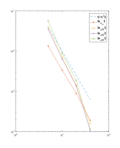
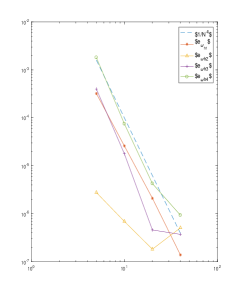
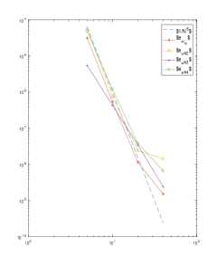
Figure 2. Relative errors for Table 3 together with the expected optimal orders, for $k=0$ (left), $k=1$ (middle) and $k=2$ (right).

From Figure 2 we confirm that for $k>0$ the discrete eigenvalues obtained are very similar to the extrapolated eigenvalue, which generates the precision errors in the correct convergence obtained.

We present in Figure 3 plots of the first and third eigenfunctions of the spectral problem in the presented configuration. The colors represent the magnitude of the displacement $\boldsymbol{u}$ of the elastic structure.

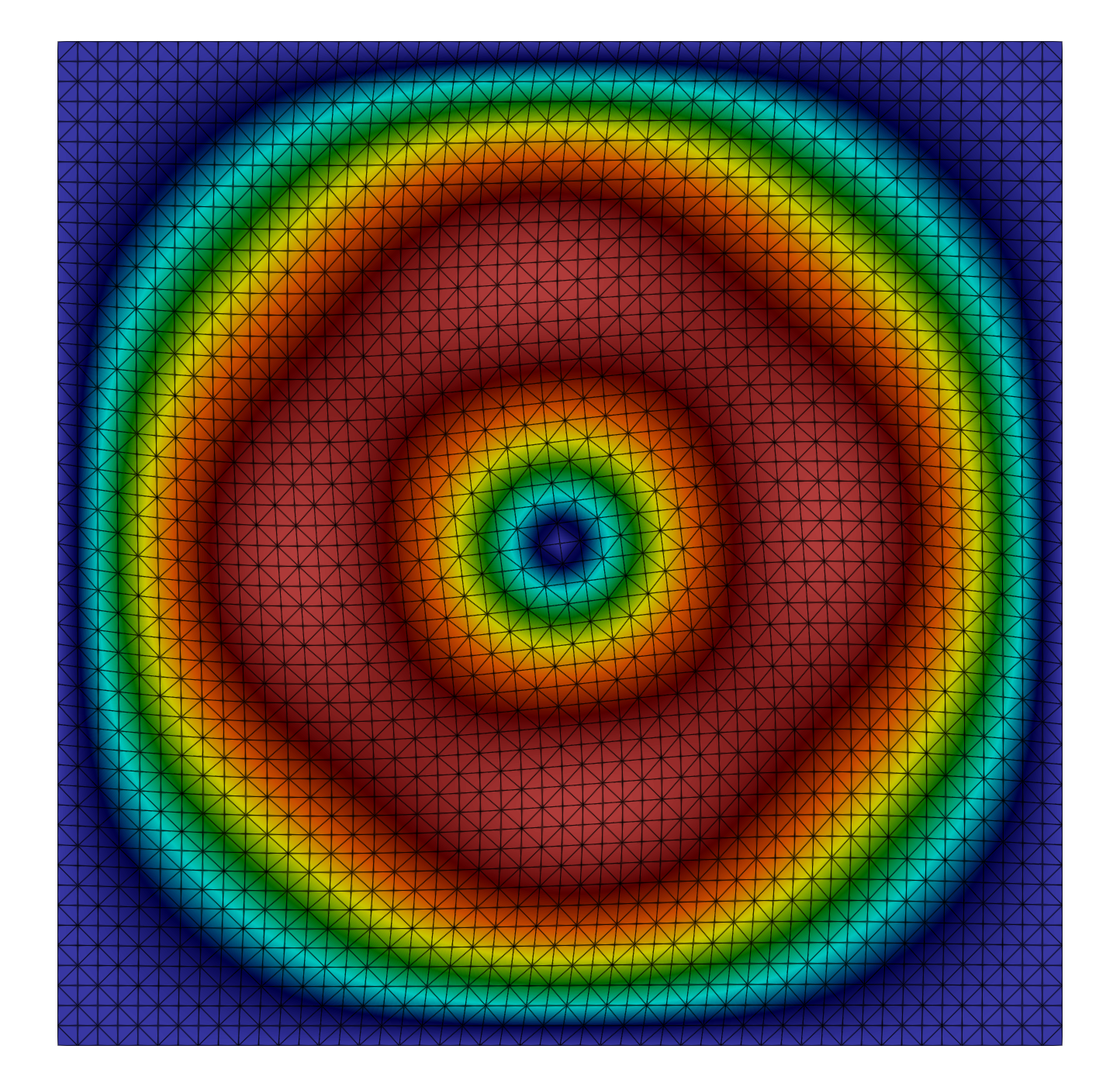
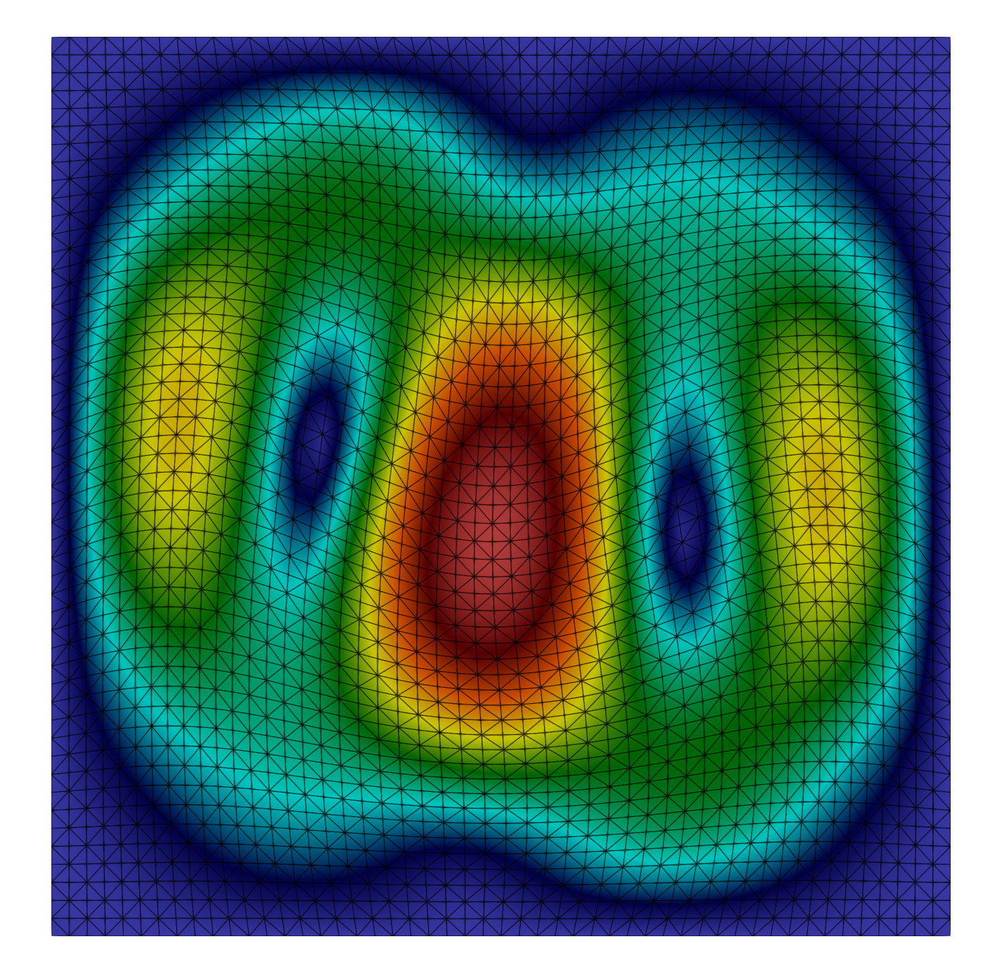
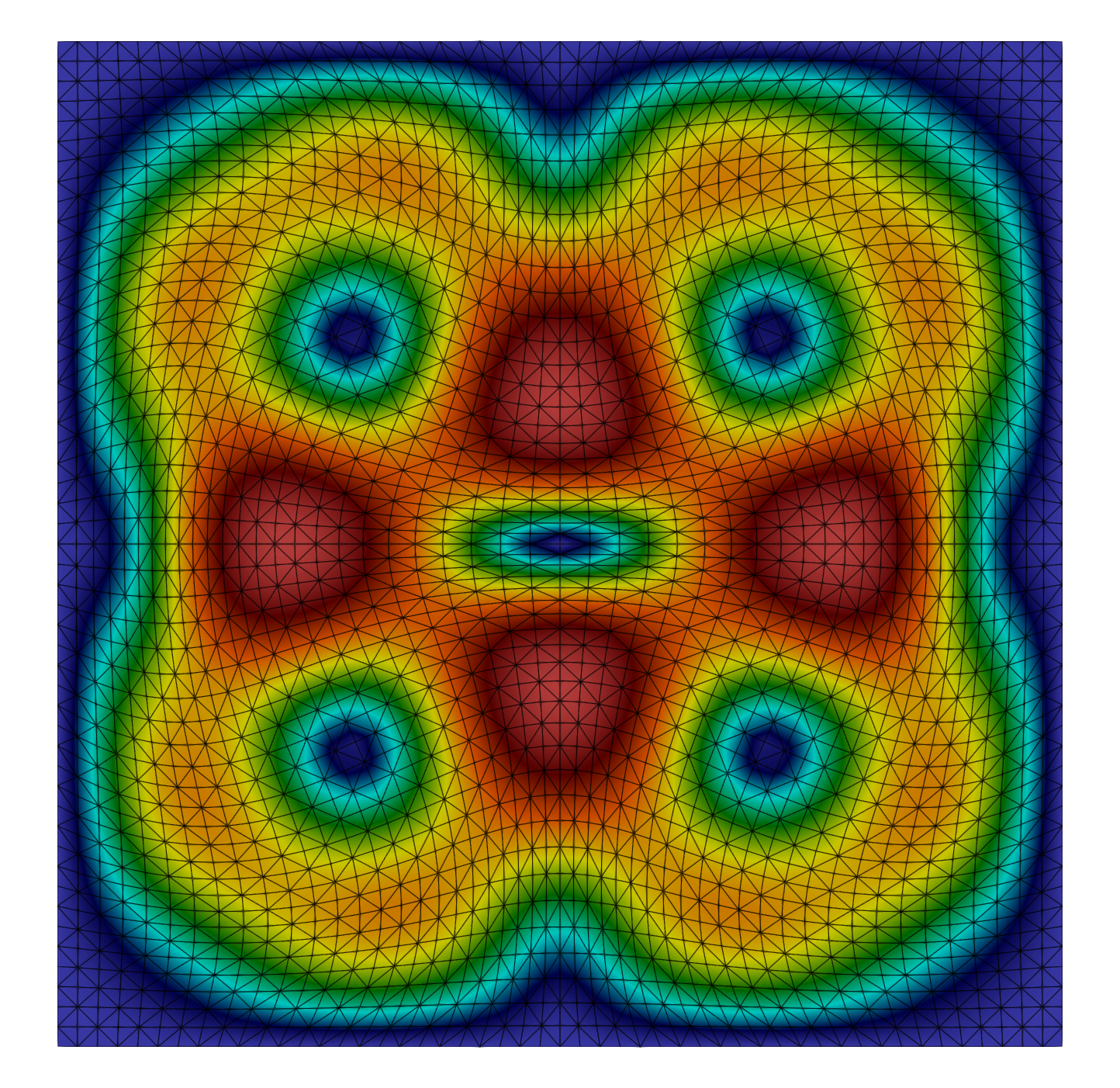
Figure 3. Eigenfunctions corresponding to the first (left), second (middle) and fourth (right) eigenvalues with $\nu=0.49$, $N=50$ and $k=1$.

5.2. Unitary cube

In the following test we consider a three dimensional domain. For simplicity, we have chosen the unitary cube $\Omega:=(0,1)^{3}$ and the lowest order finite element spaces (i.e. $k=0$). The meshes for this tests consist in regular tetrahedrons and $N$, which we consider as refinement level, corresponds to the number of tetrahedrons in the plane $XY$, with partitions respect to the $X$ axis.

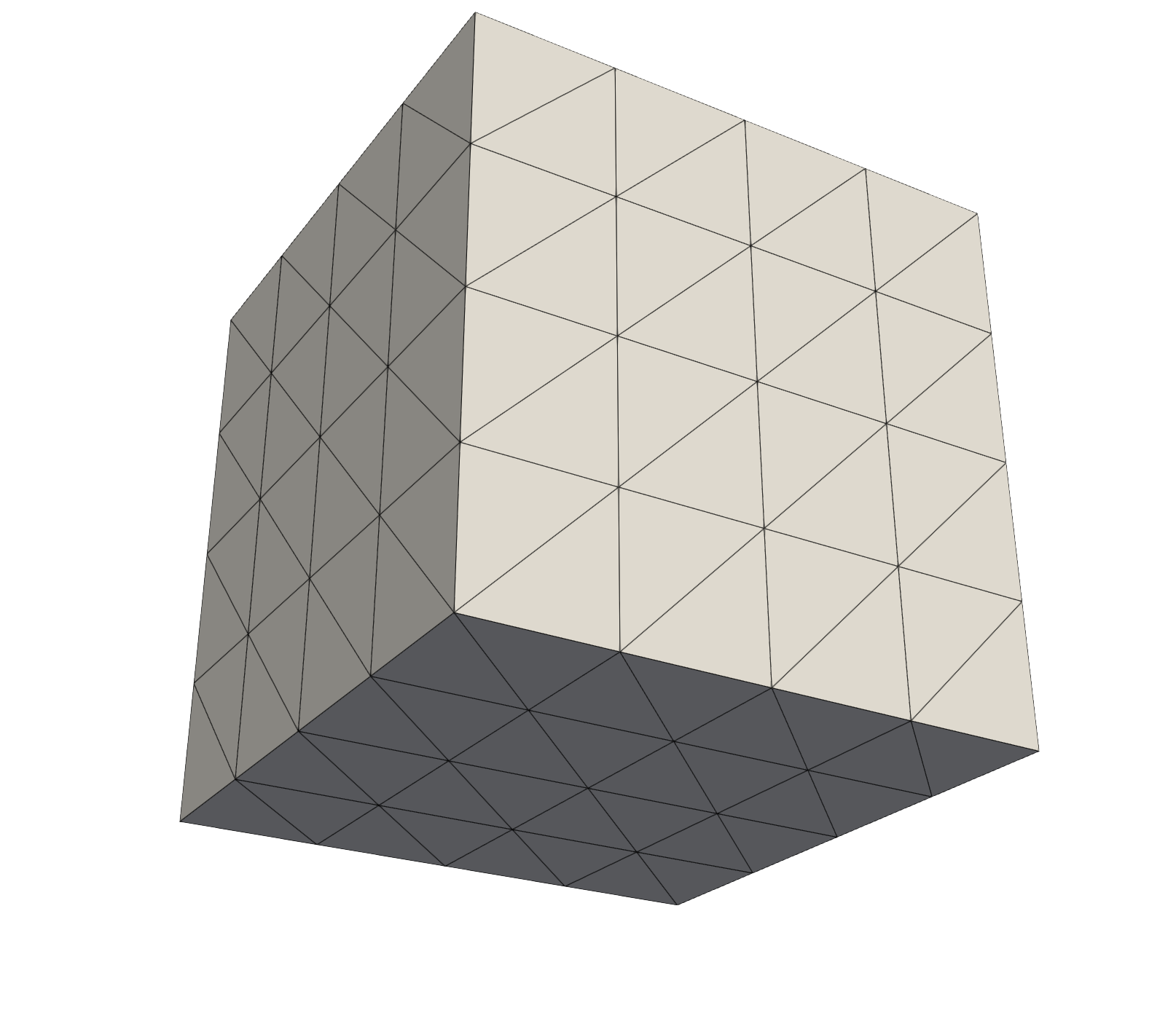
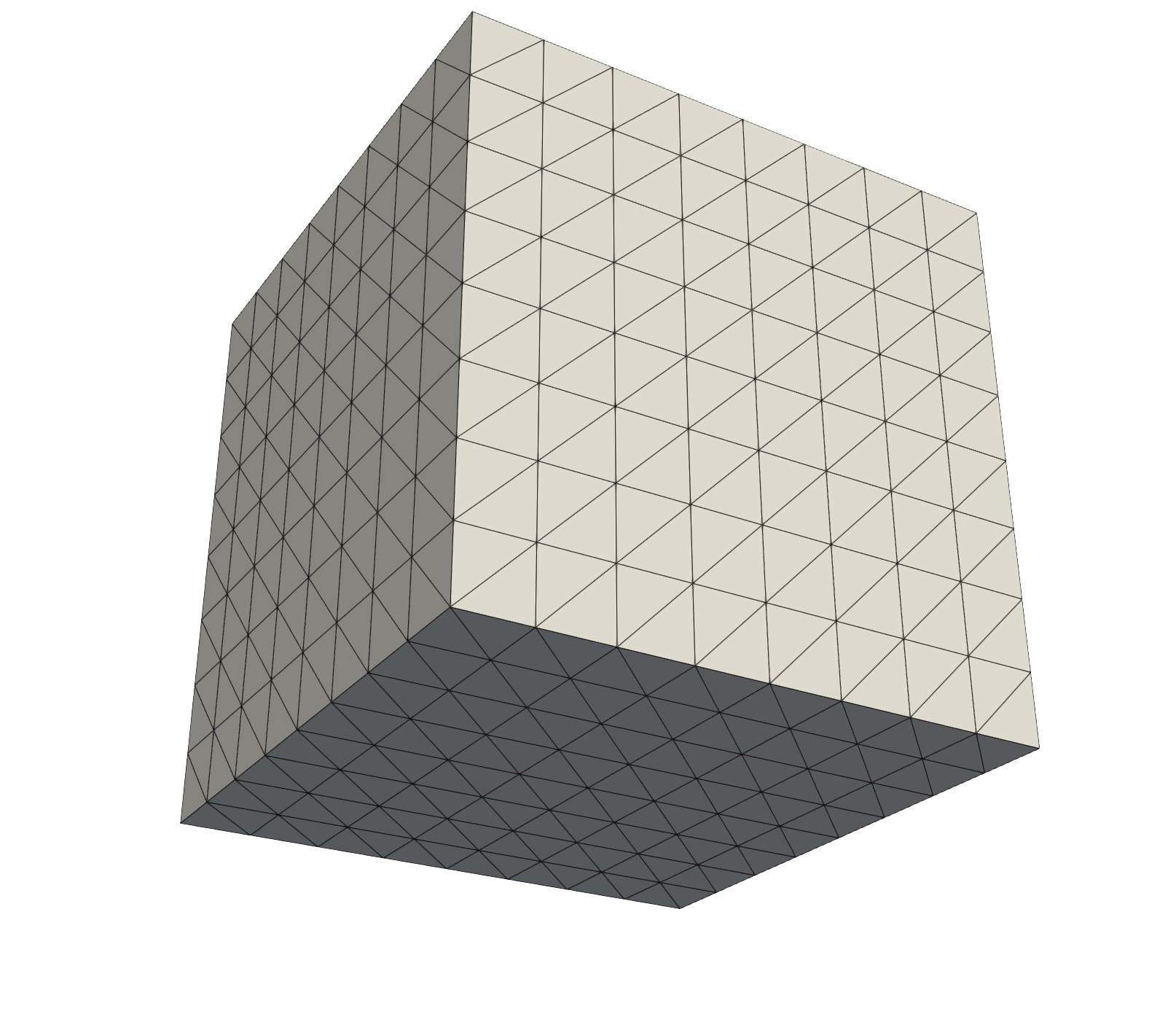
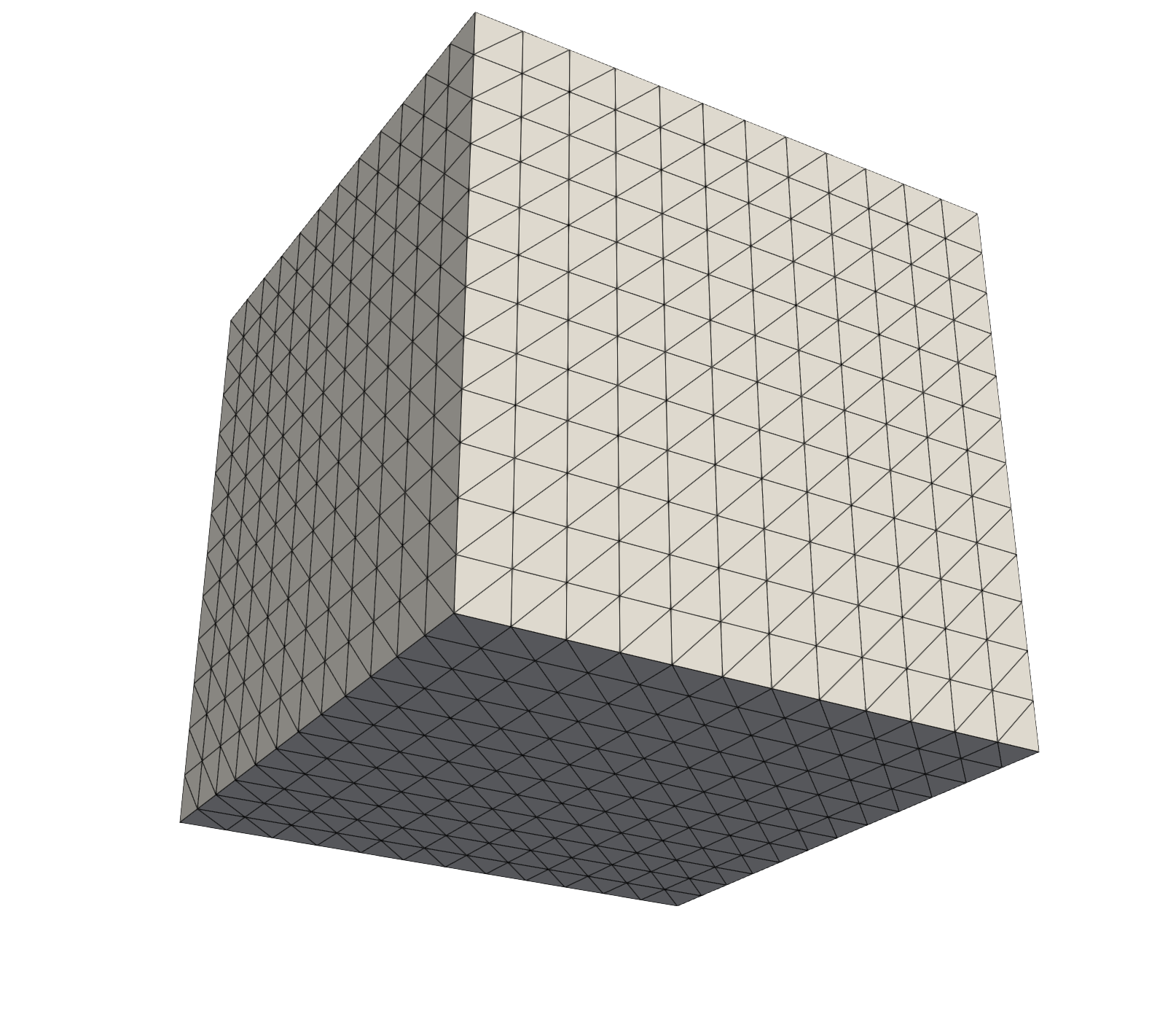
Figure 4. Examples of the meshes used in the unit cube. The left figure represents a mesh for $N=4$, the figure in for $N=8$ and the right figure for $N=12$.

In Table 4 we report the first five vibration frequencies computed for different values of $\nu$ and the corresponding orders of convergence and extrapolated values, considering the lowest order of approximation ($k=0$).

$\nu$	$N=14$	$N=16$	$N=18$	$N=20$	$\alpha$	$\omega_{extr}$
	4.43174	4.43807	4.44251	4.44573	1.83	4.46093
	4.44878	4.45122	4.45296	4.45424	1.72	4.46068
0.35	4.44878	4.45122	4.45296	4.45424	1.72	4.46068
	4.76330	4.76410	4.76617	4.76702	1.91	4.77083
	4.76645	4.76740	4.76807	4.76856	1.83	4.77085
	4.61097	4.61289	4.61423	4.61521	1.87	4.61968
	4.61396	4.61518	4.61604	4.61667	1.79	4.61970
0.45	4.61396	4.61518	4.61604	4.61667	1.79	4.61970
	5.13647	5.15367	5.16565	5.17432	1.88	5.21395
	5.17493	5.18332	5.18919	5.19345	1.85	5.21328
	4.54302	4.54513	4.54660	4.54767	1.85	4.55266
	4.54594	4.54735	4.54836	4.54909	1.76	4.55271
0.5	4.54594	4.54735	4.54836	4.54909	1.76	4.55271
	5.52484	5.52524	5.52551	5.52571	2.13	5.52646
	5.52484	5.52524	5.52551	5.52571	2.13	5.52646

Table 4. Computed lowest vibration frequencies for $k=0$ and different Poisson’s ratio in the unitary cube.

It is clear from Table 4 that the double order of convergence for the eigenvalues is obtained in this geometry setting. Also, for the limit case $\nu=0.5$, the method in the three dimensional domain works perfectly and approximates the eigenvalues with the expected double order $\mathcal{O}(h^{2})$.

In Figure 5 we present plots of the computed eigenfunctions in the unitary cube where the colors are as in the previous example. Also the plots show the deformation of the cube for each eigenfunction.

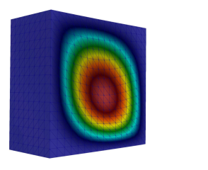
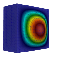
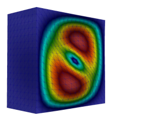
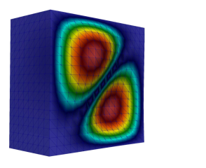
Figure 5. Eigenfunctions corresponding to the first (upper left), second and third (upper right), fourth (bottom left) and fifth (bottom right) eigenvalues, for $\nu=0.35$, $N=10$ and $k=0$.

5.3. Circular domain

For this test, we will consider as domain the unitary circle $\Omega_{C}:=\{(x,y)\in\mathbb{R}^{2}\,:\,x^{2}+y^{2}<1\}$. Clearly, with this test we are considering a particular case where we will approximate a curved domain with triangles. This geometrical features will be reflected in the order of convergence, as it happens, for instance, in [20] for the DG method.

In Tables 5, 6 and 7, the parameter $N$ represents the refinement level of each mesh that, in this case, is such that $N$ is proportional to $1/h$, where $h$ is the mesh size. In Figure 6 we present plots of some meshes for $\Omega_{C}$.

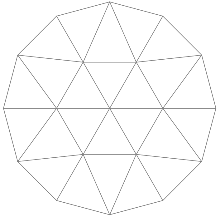
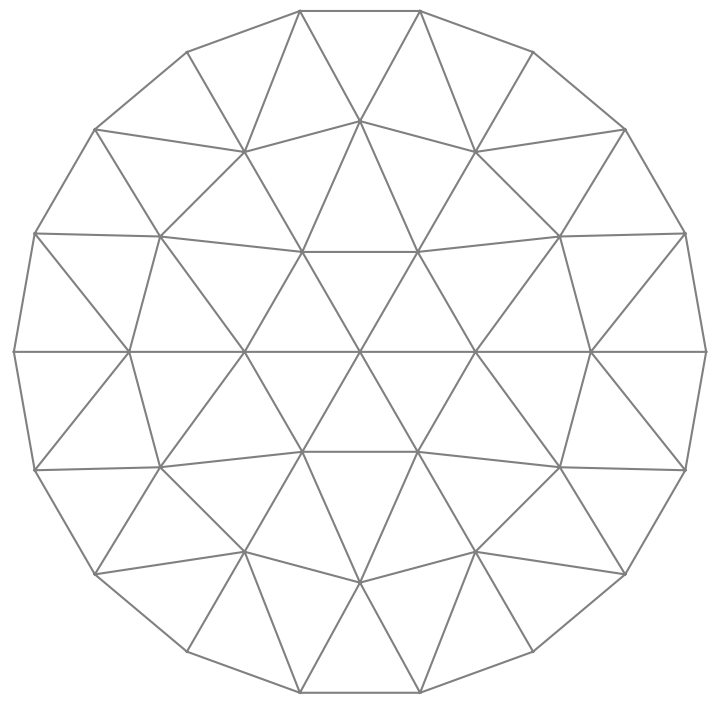
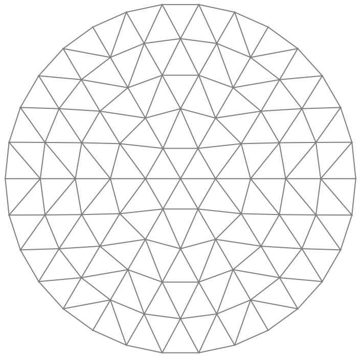
Figure 6. Examples of the meshes used in the circular domain.

In the following table we report the computed first five vibration frequencies with our method, considering different values of $\nu$ and different polynomial degrees.

$\nu$	$N=20$	$N=30$	$N=40$	$N=50$	$\alpha$	$\omega_{extr}$
	2.33142	2.33193	2.33211	2.33216	2.40	2.33225
	2.33142	2.33193	2.33211	2.33219	1.98	2.33234
0.35	2.33344	2.33250	2.33229	2.33219	2.25	2.33110
	3.32033	3.31881	3.31829	3.31805	2.02	3.31762
	3.32033	3.31881	3.31829	3.31805	2.02	3.31762
	2.22115	2.22032	2.22002	2.21989	2.00	2.21965
	2.95910	2.95854	2.95834	2.95825	1.99	2.95809
0.49	2.95910	2.95854	2.95834	2.95825	1.99	2.95809
	3.68395	3.68339	3.68319	3.68310	1.89	3.68291
	3.68395	3.68339	3.68319	3.68310	1.89	3.68291
	2.21374	2.21290	2.21261	2.21248	2.00	2.21224
	2.96637	2.96564	2.96538	2.96526	2.00	2.96505
0.5	2.96637	2.96564	2.96538	2.96526	2.00	2.96505
	3.68490	3.68419	3.68393	3.68381	1.92	3.68358
	3.68490	3.68419	3.68393	3.68381	1.92	3.68358

Table 5. Computed lowest vibration frequencies for $k=0$ and different Poisson’s ratio in the unitary circle.

$\nu$	$N=10$	$N=20$	$N=30$	$N=40$	$\alpha$	$\omega_{extr}$
	2.33244	2.33214	2.33204	2.33199	2.00	2.33190
	2.33287	2.33258	2.33247	2.33243	2.00	2.33234
0.35	2.33287	2.33258	2.33247	2.33243	2.00	2.33234
	3.31838	3.31795	3.31781	3.31774	2.01	3.31762
	3.31838	3.31795	3.31781	3.31774	2.01	3.31762
	2.22016	2.21987	2.21977	2.21973	2.00	2.21965
	2.95877	2.95839	2.95826	2.95820	2.01	2.95809
0.49	2.95877	2.95839	2.95826	2.95820	2.01	2.95809
	3.68378	3.68330	3.68314	3.68306	2.02	3.68293
	3.68378	3.68330	3.68314	3.68306	2.02	3.68293
	2.21274	2.21246	2.21236	2.21232	2.00	2.21224
	2.96573	2.96535	2.96522	2.96516	2.01	2.96505
0.5	2.96573	2.96535	2.96522	2.96516	2.01	2.96505
	3.68444	3.68396	3.68380	3.68372	2.02	3.68359
	3.68444	3.68396	3.68380	3.68372	2.02	3.68359

Table 6. Computed lowest vibration frequencies for $k=1$ and different Poisson’s ratio in the unitary circle.

$\nu$	$N=10$	$N=20$	$N=30$	$N=40$	$\alpha$	$\omega_{extr}$
	2.33243	2.33213	2.33203	2.33198	2.01	2.33190
	2.33287	2.33257	2.33247	2.33242	2.00	2.33234
0.35	2.33287	2.33257	2.33247	2.33242	2.00	2.33234
	3.31837	3.31795	3.31780	3.31773	2.00	3.31761
	3.31837	3.31795	3.31780	3.31773	2.00	3.31761
	2.22015	2.21987	2.21977	2.21972	2.01	2.21964
	2.95876	2.95839	2.95825	2.95819	2.01	2.95809
0.49	2.95876	2.95839	2.95825	2.95819	2.01	2.95809
	3.68377	3.68330	3.68313	3.68305	2.01	3.68292
	3.68377	3.68330	3.68313	3.68305	2.01	3.68292
	2.21274	2.21246	2.21236	2.21231	2.01	2.21223
	2.96573	2.96535	2.96522	2.96516	2.01	2.96505
0.5	2.96573	2.96535	2.96522	2.96516	2.01	2.96505
	3.68443	3.68396	3.68379	3.68372	2.01	3.68358
	3.68443	3.68396	3.68379	3.68372	2.01	3.68358

Table 7. Computed lowest vibration frequencies for $k=2$ and different Poisson’s ratio in the unitary circle.

We observe from tables 5, 6 and 7 that for different values of the Poisson ratio, even in the limit case when $\lambda=+\infty$, the proposed method approximates with high accuracy the eigenvalues in the circle. An important phenomena in this experiment is that, independent of the polynomial that we are considering, the order of convergence is $\mathcal{O}(h^{2})$ for any $k\geq 0$ and Poisson ratio $\nu$. We remark that we obtain these orders of convergence because of the variational crime committed by approximating the curved domain with a polygonal one.

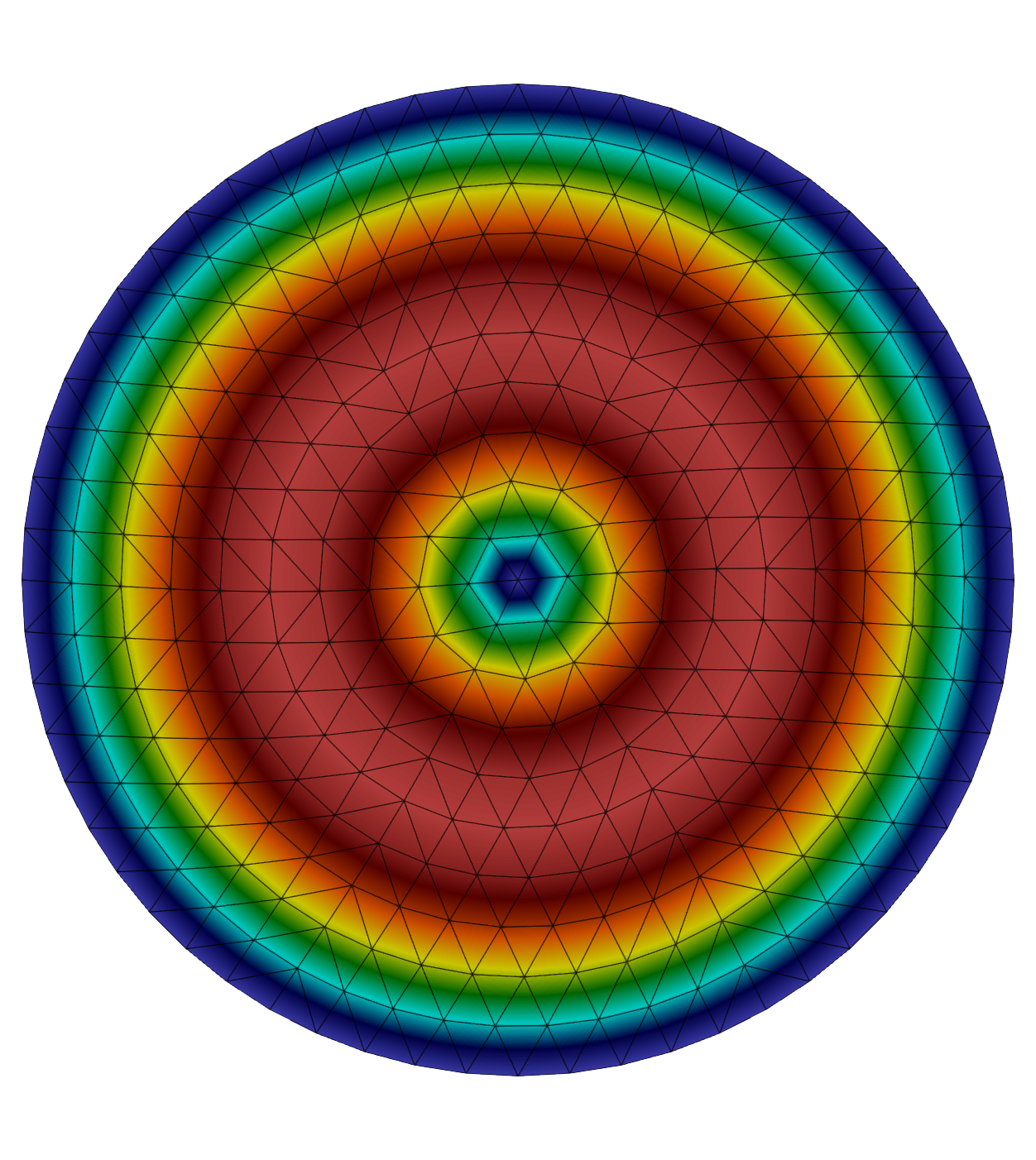
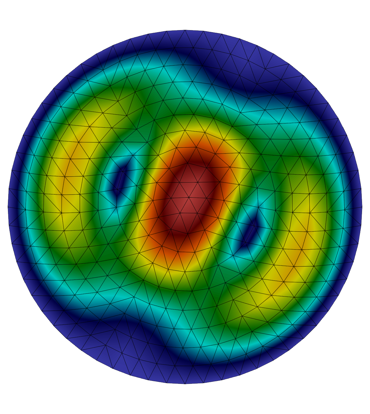
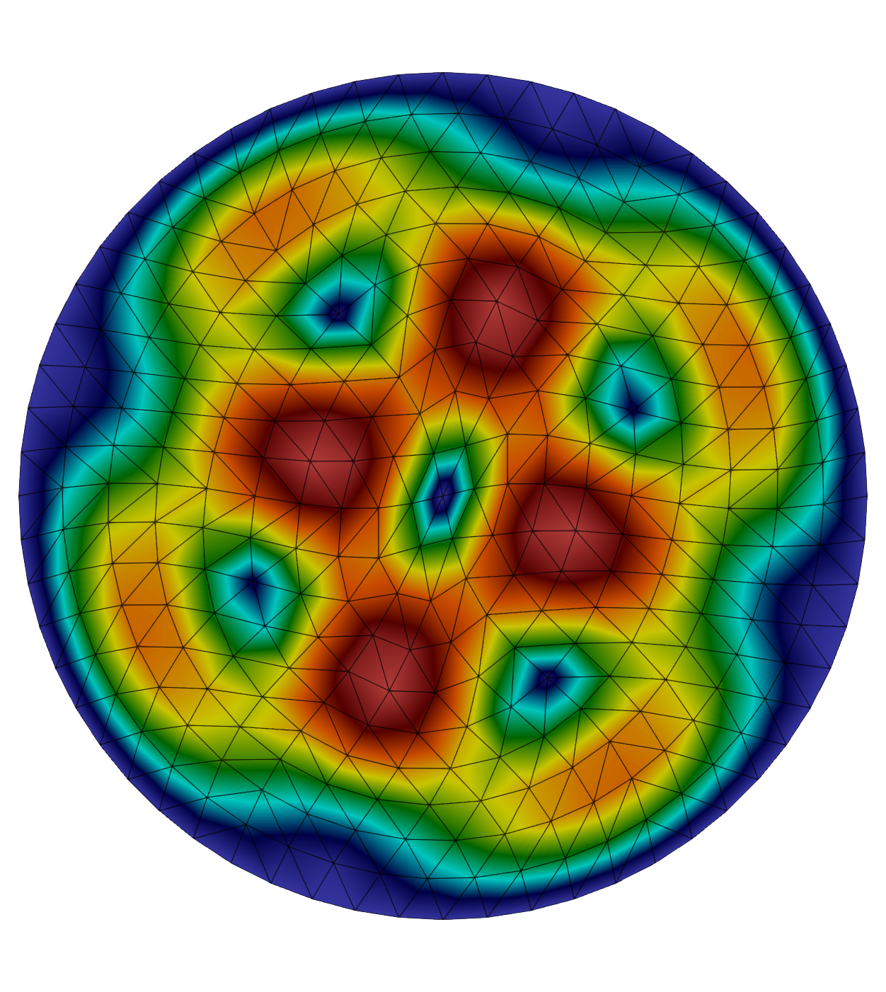
Figure 7. Eigenfunctions corresponding to the first (upper left), second and third (upper right), and fourth and fifth (bottom) computed eigenfunctions with $\nu=0.49$, $N=10$ and $k=1$.

5.4. L-shaped domain

In this section we consider a non-convex domain that we will call the L-shaped domain which is defined by $\Omega_{L}:=(-1,1)^{2}\setminus[-1,0]^{2}.$

$\nu$	$\widehat{s}$
0.35	0.6797
0.49	0.5999
0.5	0.5946

Table 8. Sobolev regularity exponents.

The eigenfunctions of this problem may present singularities due the reentrant angles of the domain. According to [15] in this case the estimate Lemma 2.1 holds true for all $s<0.5445$. Comparing this value with those of Table 8, it is observed that the strongest singularity can arise from the reentrant angle. Then, the theoretical order of convergence satisfies $2s\geq 1.08$.

In this experiment, $N$ will represent the refinement level of the meshes and it is chosen as similar to the circular domain. In tables 9, 10 and 11 we report the first five vibration frequencies obtained with our method, the respective order of convergence and extrapolates values for $\nu=0.35,0.49,0.5$ and polynomial degrees $k=0,1,2$.

$\nu$	$N=10$	$N=20$	$N=30$	$N=40$	$\alpha$	$\omega_{extr}$
	2.35882	2.37007	2.37385	2.37452	1.35	2.37768
	2.76390	2.78752	2.79281	2.79434	1.79	2.79726
0.35	3.19541	3.24358	3.26016	3.26354	1.28	3.27876
	3.56499	3.60428	3.61377	3.61600	1.74	3.62146
	3.73545	3.77218	3.78016	3.78270	1.80	3.78710
	3.17244	3.22333	3.24295	3.24667	1.15	3.26734
	3.43339	3.48637	3.49814	3.50156	1.80	3.50800
0.49	3.67087	3.70410	3.71116	3.71350	1.82	3.71731
	3.97744	4.02607	4.03584	4.03817	2.00	4.04256
	4.11516	4.17884	4.19661	4.20125	1.51	4.21421
	3.17263	3.22526	3.24565	3.24948	1.14	3.27131
	3.44052	3.49132	3.50264	3.50594	1.79	3.51223
0.5	3.70134	3.72848	3.73388	3.73579	1.89	3.73851
	3.97643	4.02421	4.03397	4.03625	1.98	4.04072
	4.22529	4.26701	4.28257	4.28629	1.13	4.30359

Table 9. Computed lowest vibration frequencies for $k=0$ and different Poisson’s ratio in the L-shaped domain.

$\nu$	$N=10$	$N=20$	$N=30$	$N=40$	$\alpha$	$\omega_{extr}$
	2.37477	2.37699	2.37774	2.37779	1.49	2.37830
	2.79548	2.79706	2.79739	2.79746	1.96	2.79761
0.35	3.26609	3.27349	3.27588	3.27605	1.53	3.27766
	3.61883	3.62068	3.62114	3.62123	1.75	3.62149
	3.78550	3.78619	3.78641	3.78642	1.60	3.78655
	3.24882	3.25954	3.26319	3.26346	1.46	3.26609
	3.50462	3.50739	3.50798	3.50814	1.87	3.50845
0.49	3.71621	3.71680	3.71700	3.71701	1.51	3.71715
	4.04169	4.04245	4.04259	4.04261	2.14	4.04267
	4.20692	4.21080	4.21184	4.21194	1.76	4.21251
	3.25169	3.26296	3.26682	3.26710	1.45	3.26991
	3.50883	3.51157	3.51216	3.51232	1.88	3.51261
0.5	3.73771	3.73839	3.73856	3.73857	1.29	3.73877
	4.03966	4.04051	4.04067	4.04070	2.13	4.04076
	4.29036.	4.29473	4.29598	4.29607	1.70	4.29679

Table 10. Computed lowest vibration frequencies for $k=1$ and different Poisson’s ratio in the L-shaped domain.

$\nu$	$N=10$	$N=20$	$N=30$	$N=40$	$\alpha$	$\omega_{extr}$
	2.37704	2.37798	2.37831	2.37833	1.44	2.37857
	2.79708	2.79752	2.79761	2.79763	1.90	2.79768
0.35	3.27366	3.27668	3.27773	3.27778	1.46	3.278538
	3.62068	3.62132	3.62148	3.62150	1.82	3.62158
	3.78619	3.78647	3.78657	3.78658	1.45	3.78665
	3.25982	3.26450	3.26619	3.26628	1.41	3.26754
	3.50741	3.50826	3.50843	3.50847	2.05	3.50854
0.49	3.71679	3.71707	3.71717	3.71718	1.35	3.71726
	4.04246	4.04263	4.04266	4.04266	2.60	4.04267
	4.21091	4.21223	4.21269	4.21272	1.43	4.21306
	3.26326	3.26821	3.27000	3.27009	1.40	3.27146
	3.51160	3.51243	3.51259	3.51263	2.08	3.51270
0.5	3.73830	3.73864	3.73877	3.73877	1.35	3.73888
	4.04053	4.04072	4.04075	4.04076	2.57	4.04076
	4.29486	4.29642	4.29699	4.29702	1.38	4.29746

Table 11. Computed lowest vibration frequencies for $k=2$ and different Poisson’s ratio in the L-shaped domain.

We observe from Tables 9, 10 and 11 that our method provides a double order of convergence for the vibration frequencies. Namely, in all cases we have $s\thickapprox 2\min\{r,k+1\}$, which corresponds to the the best possible order of convergence for this problem.

We end this section presenting plots of the first three eigenfunctions obtained with our method in the L-shaped domain. In particular, we show the eigenfunctions computed with $\nu=0.35$, $k=1$ as polynomial degree and $N=10$.

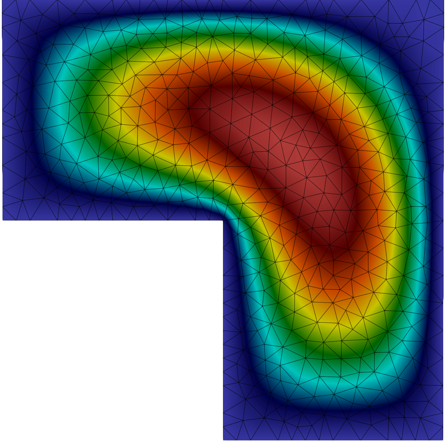
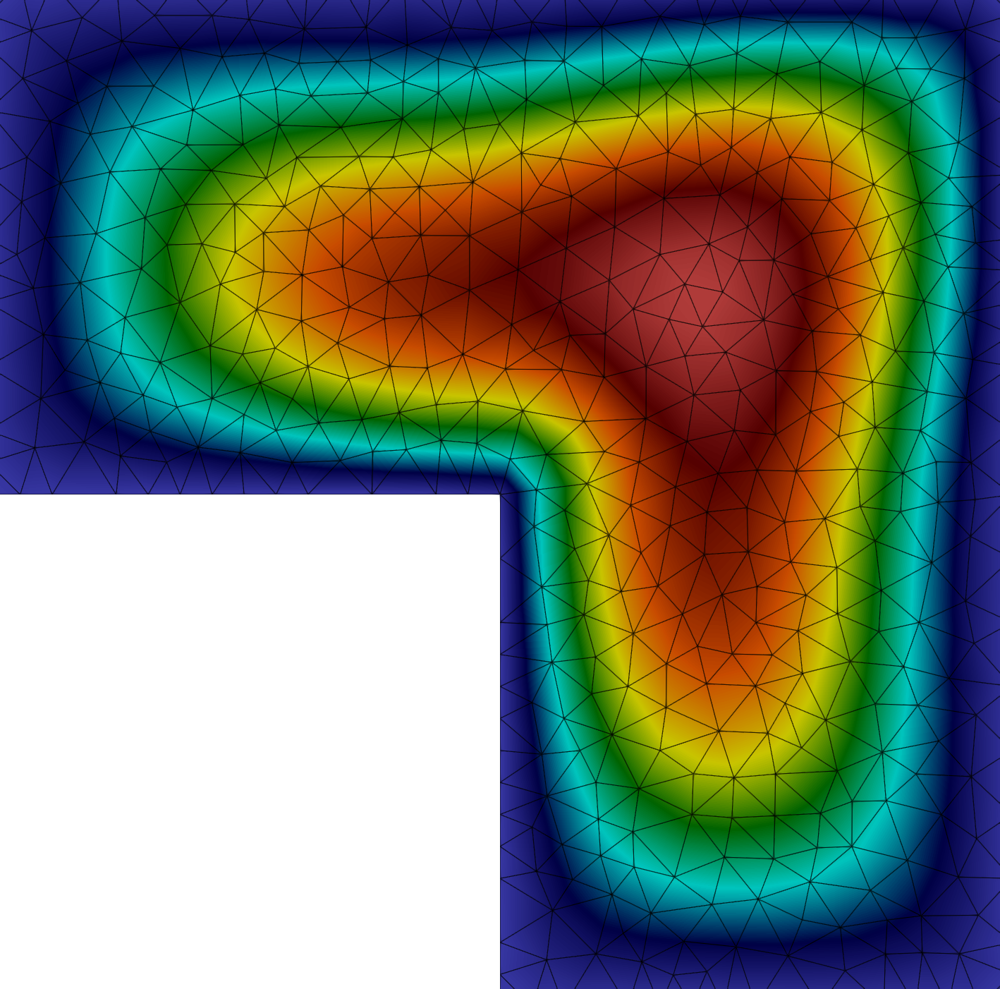
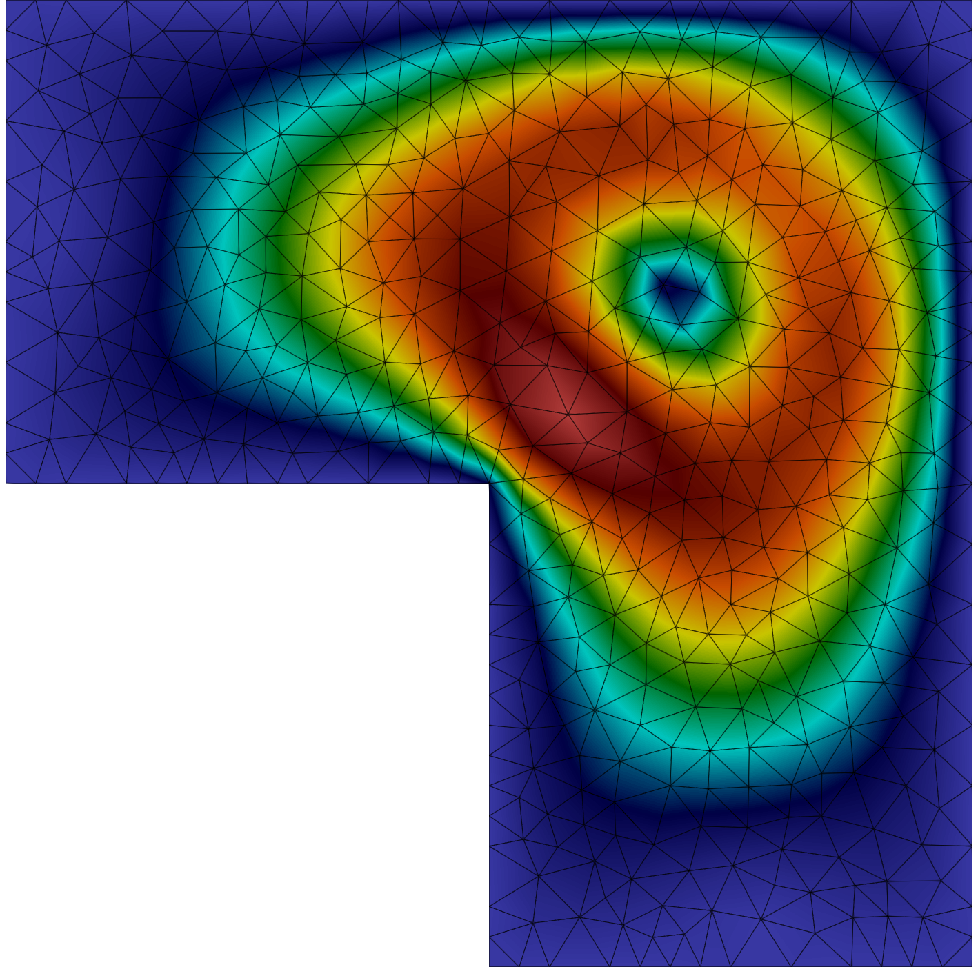
Figure 8. Eigenfunctions corresponding to the first (upper left), second (middle) and third (right) computed eigenfunctions with $\nu=0.35$, $N=10$ and $k=1$.

References

- [1] I. Babuška and J. Osborn, Eigenvalue problems, in Handbook of numerical analysis, Vol. II, Handb. Numer. Anal., II, North-Holland, Amsterdam, 1991, pp. 641–787.
- [2] L. Beirão da Veiga, D. Mora, G. Rivera, and R. Rodríguez, A virtual element method for the acoustic vibration problem, Numer. Math., 136 (2017), pp. 725–763.
- [3] F. Bertrand, D. Boffi, and R. Stenberg, Asymptotically exact a posteriori error analysis for the mixed Laplace eigenvalue problem, Comput. Methods Appl. Math., 20 (2020), pp. 215–225.
- [4] D. Boffi, F. Brezzi, and M. Fortin, Mixed finite element methods and applications, vol. 44 of Springer Series in Computational Mathematics, Springer, Heidelberg, 2013.
- [5] D. Boffi and R. Stenberg, A remark on finite element schemes for nearly incompressible elasticity, Comput. Math. Appl., 74 (2017), pp. 2047–2055.
- [6] E. Cáceres, G. N. Gatica, and F. A. Sequeira, A mixed virtual element method for a pseudostress-based formulation of linear elasticity, Appl. Numer. Math., 135 (2019), pp. 423–442.
- [7] Z. Cai, C. Tong, P. S. Vassilevski, and C. Wang, Mixed finite element methods for incompressible flow: stationary Stokes equations, Numer. Methods Partial Differential Equations, 26 (2010), pp. 957–978.
- [8] C. Carstensen, M. Eigel, and J. Gedicke, Computational competition of symmetric mixed FEM in linear elasticity, Comput. Methods Appl. Mech. Engrg., 200 (2011), pp. 2903–2915.
- [9] R. G. Durán, L. Gastaldi, and C. Padra, A posteriori error estimators for mixed approximations of eigenvalue problems, Math. Models Methods Appl. Sci., 9 (1999), pp. 1165–1178.
- [10] G. N. Gatica, L. F. Gatica, and F. A. Sequeira, A priori and a posteriori error analyses of a pseudostress-based mixed formulation for linear elasticity, Comput. Math. Appl., 71 (2016), pp. 585–614.
- [11] G. N. Gatica, A. Márquez, and M. A. Sánchez, Analysis of a velocity-pressure-pseudostress formulation for the stationary Stokes equations, Comput. Methods Appl. Mech. Engrg., 199 (2010), pp. 1064–1079.
- [12] , Pseudostress-based mixed finite element methods for the Stokes problem in with Dirichlet boundary conditions. I: A priori error analysis, Commun. Comput. Phys., 12 (2012), pp. 109–134.
- [13] V. Girault and P.-A. Raviart, Finite element methods for Navier-Stokes equations, vol. 5 of Springer Series in Computational Mathematics, Springer-Verlag, Berlin, 1986. Theory and algorithms.
- [14] J. Gopalakrishnan and J. Guzmán, Symmetric nonconforming mixed finite elements for linear elasticity, SIAM J. Numer. Anal., 49 (2011), pp. 1504–1520.
- [15] P. Grisvard, Problèmes aux limites dans les polygones. Mode d’emploi, EDF Bull. Direction Études Rech. Sér. C Math. Inform., (1986), pp. 3, 21–59.
- [16] R. Hiptmair, Finite elements in computational electromagnetism, Acta Numer., 11 (2002), pp. 237–339.
- [17] T. Kato, Perturbation theory for linear operators, Die Grundlehren der mathematischen Wissenschaften, Band 132, Springer-Verlag New York, Inc., New York, 1966.
- [18] H. P. Langtangen and A. Logg, Solving PDEs in Python, vol. 3 of Simula SpringerBriefs on Computing, Springer, Cham, 2016. The FEniCS tutorial I.
- [19] F. Lepe, S. Meddahi, D. Mora, and R. Rodríguez, Mixed discontinuous Galerkin approximation of the elasticity eigenproblem, Numer. Math., 142 (2019), pp. 749–786.
- [20] F. Lepe and D. Mora, Symmetric and nonsymmetric discontinuous Galerkin methods for a pseudostress formulation of the Stokes spectral problem, SIAM J. Sci. Comput., 42 (2020), pp. A698–A722.
- [21] F. Lepe and G. Rivera, A priori error analysis for a mixed VEM discretization of the spectral problem for the Laplacian operator, Calcolo, 58 (2021), pp. Paper No. 20, 30.
- [22] A. Márquez, S. Meddahi, and T. Tran, Analyses of mixed continuous and discontinuous Galerkin methods for the time harmonic elasticity problem with reduced symmetry, SIAM J. Sci. Comput., 37 (2015), pp. A1909–A1933.
- [23] S. Meddahi, D. Mora, and R. Rodríguez, Finite element spectral analysis for the mixed formulation of the elasticity equations, SIAM J. Numer. Anal., 51 (2013), pp. 1041–1063.
- [24] D. Mora and G. Rivera, A priori and a posteriori error estimates for a virtual element spectral analysis for the elasticity equations, IMA J. Numer. Anal., 40 (2020), pp. 322–357.
- [25] D. Mora, G. Rivera, and R. Rodríguez, A virtual element method for the Steklov eigenvalue problem, Math. Models Methods Appl. Sci., 25 (2015), pp. 1421–1445.