Efficient evader detection in mobile sensor networks

Abstract.

Suppose one wants to monitor a domain with sensors each sensing small ball-shaped regions, but the domain is hazardous enough that one cannot control the placement of the sensors. A prohibitively large number of randomly placed sensors would be required to obtain static coverage. Instead, one can use fewer sensors by providing only mobile coverage, a generalization of the static setup wherein every possible intruder is detected by the moving sensors in a bounded amount of time. Here, we use topology in order to implement algorithms certifying mobile coverage that use only local data to solve the global problem. Our algorithms do not require knowledge of the sensors’ locations. We experimentally study the statistics of mobile coverage in two dynamical scenarios. We allow the sensors to move independently (billiard dynamics and Brownian motion), or to locally coordinate their dynamics (collective animal motion models). Our detailed simulations show, for example, that collective motion enhances performance: The expected time until the mobile sensor network achieves mobile coverage is lower for the D’Orsogna collective motion model than for the billiard motion model. Further, we show that even when the probability of static coverage is low, all possible evaders can nevertheless be detected relatively quickly by mobile sensors.

1. Introduction

Suppose we would like to monitor a given domain with a network of sensors. In certain important situations, we may not be able to prescribe exact locations for the sensors. Fallen rubble might render a domain difficult to access. Monitoring forest fires requires navigating hazardous domains. Further, the sensors may have limited capabilities. We assume that each sensor can detect objects only within a ball of small radius. In such situations, placing the sensors randomly may yield static coverage, meaning that the domain is covered at a single moment in time by the union of the sensing balls. The statistics underlying random static coverage have been extensively studied [14]. Surprisingly, we can use topological techniques to verify when a random placement of sensors produces static coverage, even if the sensor positions are not known! Indeed, the network connectivity of the sensors alone is sufficient input [8].

The number of randomly placed sensors required for static coverage may be prohibitively large. Further, environmental dynamics, such as those produced by wind or ocean currents, may cause sensors to move. We therefore study mobile coverage, a type of dynamic coverage that often requires significantly fewer sensors than its static counterpart. Indeed, we consider mobile sensor networks wherein the sensors may move deterministically or stochastically. By mobile coverage we mean that no possible intruder could continuously move in the domain under surveillance without at some point being seen by at least one of the moving sensors. These sensors may achieve mobile coverage even in the absence of static coverage — i.e. even if the entire domain is never covered at any fixed moment in time by the union of the sensing balls.

Subtle topological tools exist that guarantee mobile coverage, even if the sensors are not able to monitor their position coordinates. Using these tools as a foundation, we here initiate the study of the statistics of mobile coverage in minimal mobile sensor networks. By minimal, we mean that we do not know the locations of the sensors. As a consequence, we must verify mobile coverage using only local data. This local data consists of connectivity information (overlapping sensors can detect each other), weak angular data (sensors can measure cyclic orderings of neighbors), and distance data (each sensor can measure distances to nearby detected sensors). We address the following statistical questions. Given randomly placed sensors which then move deterministically or stochastically in a domain, how do the statistics of the (random) mobile coverage time $T_{\max}$, the time at which mobile coverage is achieved, behave? Additionally, how do the mean and variance of $T_{\max}$ depend on the sensor dynamics?

We provide concrete algorithms that certify mobile coverage and use them to examine several models of sensor motion; see [1] for code and documentation. These models fall into one of two categories — either the sensors move independently, or they locally coordinate their dynamics. We examine two models wherein the sensors move independently, one deterministic (billiard motion) and one stochastic (Brownian motion). Inspired by the emergent dynamics associated with collective animal motion, we study the seminal D’Orsogna model [11] as well. In this model, sensors use local attractive and repulsive forces to coordinate motion.

As an example application, suppose that deploying a sensor requires a fixed cost, and that having the sensors turned on while roving requires a marginal cost. What is the cheapest way to achieve coverage? Is it cheaper to try and achieve static coverage, by deploying enough randomly-placed sensors to cover the domain at the start time with high probability? Or, is it cheaper to deploy fewer sensors, which likely will not cover the domain initially, but will provide mobile coverage after a certain duration of wandering? How many mobile sensors do we expect to be the most cost-efficient? Our simulations aim to allow us to answer such questions.

We survey related work in Section 2, discuss mobile coverage problems and theoretical tools in Section 3, and introduce our algorithms in Sections 4 and 5. We examine how mobile sensor network performance statistics depend on the dynamics of the mobile sensors in Sections 6 and 7. We finish with open questions and concluding remarks in Section 8.

2. Related Work

2.1. Topological approaches to minimal sensing problems

Studying mobile coverage in minimal mobile sensor networks requires using local data to solve a global problem. Topological techniques naturally facilitate local-to-global analysis. See [10] for an overview of the topological approach.

Two of the papers introducing coverage problems in sensor networks from the topological perspective are by de Silva and Ghrist. In [8], the authors consider a wide variety of sensor models (static sensors, mobile sensors) and problems (detecting static coverage, detecting mobile coverage, identifying and turning off redundant sensors). They show how coordinate-free connectivity data, when combined with homology, can address this diverse spectrum of problems. In [9], the authors incorporate persistent homology in order to obtain more refined coverage guarantees.

The mobile sensor coverage we consider in this paper is derived from Section 11 of [8]. In particular, the authors derive a one-sided criterion using relative homology, which can guarantee the existence of mobile coverage, but which cannot be used to show the nonexistence therof. In [3], Adams and Carlsson develop a streaming version of this one-sided criterion using zigzag persistence. Zigzag persistent homology can be used for hole identification, tracking, and classification in coordinate-free mobile sensor networks as well [12]. Returning to [3], Adams and Carlsson also show that whereas connectivity data alone can determine if and only if static coverage exists, time-varying connectivity data alone cannot determine whether or not mobile coverage exists. As a result, the authors augment the connectivity data by considering planar sensors that also measure distances to overlapping neighbors as well as their cyclic orderings. We consider exactly this type of minimal mobile sensor network.

We can model a mobile sensor network as two sets in space-time: a covered region and an uncovered region. The map to time can be thought of as a real-valued function, whose domain we often restrict to be only the uncovered region. The Reeb graph of the uncovered region, equipped with this real-valued map to time, encodes the space of possible (undetected) intruder motions. From this Reeb graph, it is easy to determine whether or not an evasion path exists. Our algorithms in this paper allow us to not only detect whether an evasion path exists or not, but also to compute the entire Reeb graph of the uncovered region.

In a more theoretical direction, the papers [13, 4] give if-and-only-if criteria for the existence of an evasion path using positive homology and Morse theory, but do not address how minimal sensors would measure the inputs required for these criteria. For example, the input required to compute the example in Section 6 of [13] is enough information to instead directly compute the Reeb graph of the uncovered region. The papers [2, 3, 4] raise and partially address the problem of computing the entire space of evasion paths, which in [19] is implemented for planar sensors that can measure cyclic orderings of and local distances to nearby sensors. Though [19] assumes that each sensor knows its positional coordinates, this assumption can be slightly weakened: if instead each sensor only knows which sensors it overlaps with, and the exact distances to overlapping sensors, then this is enough information to compute alpha complexes.

2.2. Static coverage

What is the probability that immobile ball-shaped sensors cover a domain, or equivalently, what is the probability that mobile ball-shaped sensors cover a domain at time zero? These static coverage questions have a long history in statistics and mathematics. Sections 1.6 and 3.7 of [14] discuss both upper and lower bounds on the probability of coverage by $n$ sensors, and  [30] addresses moment problems related to static coverage. Exact formulas for the probability of coverage by a fixed number of sensors are typically unknown. Instead, it is common to take a limit where the number of sensors goes to infinity while their radii go to zero. Kellerer [17] considers the expected number of connected components of a random sample of balls, as well as the expected Euler characteristic. For connections between static coverage and the properties of convex hulls of multivariate samples, see [24].

2.3. A panoply of mobile sensor network models

It is possible to vary the set-up of the pursuit-evasion mobile sensor network problems that are considered here in countless ways. For instance, we deem an evader to have been detected at the instant it enters a sensing ball. Liu, Dousse, Nain, and Towsley [22] require that the evader remain in a given sensing ball for a certain amount of time in order for detection to occur. They show in this context that sensors should not move too quickly if we wish to optimize mobile sensor network performance. We assume that sensor motion and evader motion are independent. One could instead study intelligent sensor networks wherein sensor trajectories actively respond to evader dynamics. We assume that evaders can move arbitrarily fast, provided their motion remains continuous. One could impose constraints on evader motion (such as bounded speed) and then ask a number of intriguing questions. Given a set of constraints on evader motion, what is the optimal evasion strategy? How can game theory inform our understanding of the pursuit-evasion problem if both evaders and sensors are intelligent? See [7] for a taxonomy of pursuit-evasion problems and [5, 21, 22] for game-theoretic approaches.

A variety of ideas have been harnessed to analyze mobile sensor networks. From a control theory perspective, flocking algorithms have been combined with Kalman filters for efficient target tracking [20, 25, 26, 27, 28, 31, 32]. The collective behavior of the ant species Temnothorax albipennis has inspired distributed coordination algorithms for tracking [33]. Neural networks can learn a priori unknown environments while dynamic coverage is achieved [29].

3. Mobile coverage problems and theoretical tools

Let $D\subset\mathbb{R}^{2}$ be a compact domain that is homeomorphic to a closed disk. We assume that the boundary $\partial D$ is piecewise-smooth. Let $X\subset D$ be a finite set of sensor locations. We equip the sensors with a sensing radius $r$, within which they can detect intruders and other sensors. More precisely, each sensor $x\in X$ covers a ball $B_{r}(x)=\{y\in\mathbb{R}^{2}:\|y-x\|\leqslant r\}$. Sensor $x$ immediately detects any intruder or sensor inside this sensing ball. We further assume that there exists a subset of immobile fence sensors, $F\subset X$, such that $\partial D\subset\cup_{x\in F}B_{r}(x)$. We may think of these fence sensors as being on the boundary, though this is not strictly necessary.

The covered region of the sensors is the set $C=D\cap(\cup_{x\in X}B_{r}(x))$. The static coverage problem asks if $D=C$ (equivalently, if $D\setminus C=\emptyset$). We do not need to know the coordinates of the sensors in order to address this problem. Indeed, using only sensor connectivity data as input, de Silva and Ghrist [8] formulate homological conditions that guarantee static coverage.

3.1. Mobile coverage

This paper focuses on mobile coverage problems, wherein sensors are allowed to move. We modify the static setup as follows. Let $I=[0,T]$ parametrize time, for some fixed maximum value $T>0$. Each sensor now traces a continuous path $x\colon I\to D$. Let $\mathscr{X}$ denote the collection of these paths. As in the static case, we assume there exists a subset of $\mathscr{X}$ corresponding to fence sensors. The fence sensors are immobile, meaning $x(t)=x(t^{\prime})$ for all $t,t^{\prime}\in I$ if $x$ is a fence sensor. We continue to assume that the boundary $\partial D$ is covered by the sensing balls of these (static) fence sensors.

We are interested in the ability of the mobile sensor network to detect all possible continuously moving intruders.

Definition 3.1.

The time-varying covered region is $C(t)=D\cap(\cup_{x\in\mathscr{X}}B_{r}(x(t)))$ for $t\in I$. An evasion path in the mobile sensor network is a continuous path $p\colon I\to D$ with $p(t)\notin C(t)$ for all $t\in I$. We say that a mobile sensor network exhibits mobile coverage on $D\times I$ if no evasion path exists.

Note that we make no assumptions about the modulus of continuity of the evasion paths. In particular, we place no bound on the speed at which a potential evader may travel. An intruder successfully avoids detection by simply moving continuously and never falling into the time-varying covered region. Our problem of mobile coverage is really a question about the existence of evasion paths.

Problem 3.2.

Fix $T>0$. Given sensor paths $(x_{n})$, determine if an evasion path exists on $D\times[0,T]$.

We extend Problem 3.2 by not fixing $T$ in advance, but rather asking for the maximal time interval over which an evasion path exists.

Problem 3.3.

Given sensor paths $(x_{n})$, find the detection time

$$T_{\max}=\sup\{T\geqslant 0:\text{there exists an evasion path on }D\times[0,T]\}.$$

These mobile coverage problems motivate our two primary goals. First, we want to develop efficient algorithms that solve these mobile coverage problems using as little information as possible about the sensor paths. Our second goal is to understand how the statistics of this detection time depend on sensor dynamics, the number of sensors, the sensing radius, and the geometry of the domain $D$.

Suppose that each sensor can measure the cyclic ordering of its neighbors. If the sensor network remains connected at each time and if the sensors can measure the time-varying alpha complex, then there exists an if-and-only-if criterion for the existence of an evasion path [3, Theorem 3]. In this paper, the authors also outline a constructive method for determining the existence of these evasion paths. We now give the necessary background material to make this algorithm explicit.

3.2. The alpha complex

Fix a finite set $X$ of points in $\mathbb{R}^{2}$ (the sensor positions at a fixed time). For any $x\in X$, the Voronoi region $V_{x}\subset\mathbb{R}^{2}$ is defined as

$$V_{x}=\left\{y\in\mathbb{R}^{2}:\|y-x\|\leqslant\|y-x^{\prime}\|\text{ for all }x^{\prime}\in X\setminus\{x\}\right\}.$$

That is, the Voronoi region about $x$ contains all points in the plane that are as close to $x$ as they are to any other point in $X$. For example, if $X=\{x,x^{\prime}\}$ consists of two points in the plane, then each Voronoi region will be a half-space, with the perpendicular bisector of the line segment $xx^{\prime}$ as the line dividing the two half-spaces.

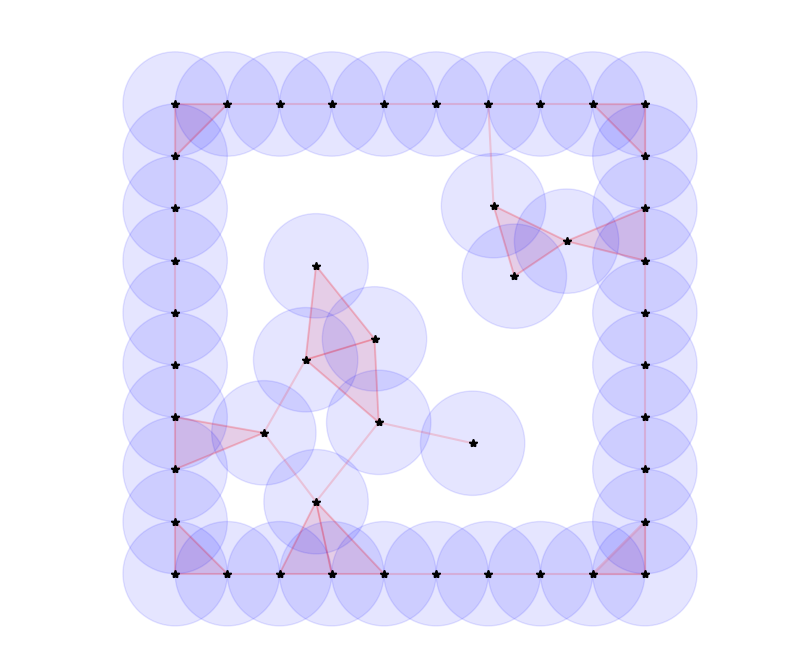
Figure 1. Alpha complex produced by a mobile sensor network at a fixed time. Black stars denote sensor positions and shaded disks depict sensing balls. Line segments and shaded triangles represent 1-simplices and 2-simplices in the alpha complex, respectively.

Each sensor $x\in X$ covers a closed ball $B_{r}(x)$ of radius $r$. The alpha complex of $X$ is defined as follows. Consider the convex regions $B_{r}(x)\cap V_{x}$ obtained by intersecting the closed ball of radius $r$ about $x$ with the Voronoi region corresponding to $x$. The alpha complex is a simplicial complex, with vertex set $X$, that contains a $(k-1)$-simplex if the corresponding $k$ convex regions $B_{r}(x)\cap V_{x}$ have a point of mutual intersection; see Figure 1 for an example. In particular, we have a vertex (i.e. a 0-simplex) in the alpha complex for each convex region $B_{r}(x)\cap V_{x}$, i.e. we have a vertex for each point $x\in X$. We have an edge (i.e. a 1-simplex) $xx^{\prime}$ in the alpha complex whenever two convex regions $B_{r}(x)\cap V_{x}$ and $B_{r}(x^{\prime})\cap V_{x^{\prime}}$ intersect. When three such regions share a point of intersection, we have a triangle (i.e. a 2-simplex) in the alpha complex. By the nerve lemma [15, Corollary 4G.3], the alpha complex is homotopy equivalent to the union of the convex regions $B_{r}(x)\cap V_{x}$, which is the same space as the union of the sensing balls $B_{r}(x)$ (i.e. the covered region).

The alpha complex can be determined from only the pairwise distances between sensors whose corresponding sensing balls overlap; see the proof in Appendix A. This is local data — we do not need to know the distances between non-overlapping sensing balls in order to compute the alpha complex. Hence we can use alpha complexes in minimal sensing algorithms.

3.3. Fat graphs and boundary cycles

A fat graph [16, 23] is a graph equipped with a cyclic ordering of the directed edges about each of its vertices. Using the cyclic ordering, the directed edges can be partitioned into closed loops known as boundary cycles. These boundary cycles will be used to identify connected components of both the covered and uncovered region. This translation from cyclic information about vertices to boundary cycles is useful in our study of mobile planar sensor networks for the following reason: cyclic orderings of neighbors can be detected by sensors with minimal capabilities because this information is local in nature. For example, each sensor could use a rotating radar tower to order its neighbors. By contrast, boundary cycles are global in nature, and some of these boundary cycles correspond to holes in the sensor network. Therefore, by using the translation from rotation information to boundary cycles, we are able to convert local data measured by sensors into global data representing the connected components of the uncovered region.

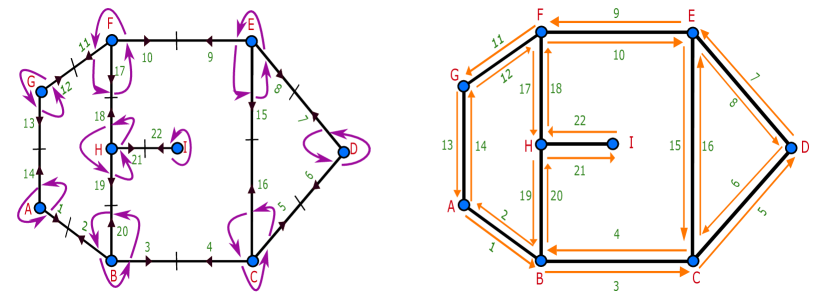
Figure 2. An example fat graph (left) along with its boundary cycles (right).

Figure 2 (left) depicts a sample fat graph equipped with labels on its vertices and half-edges. Each half-edge is oriented. For example, $1$ denotes the half-edge from vertex $A$ to $B$, whereas $2$ denotes the half-edge from $B$ to $A$. Given a fat graph, we have an involution $\alpha$ that acts on the half-edges by reversing orientation, as well as a bijection $\sigma$ that returns the next half-edges about a vertex in a counter-clockwise direction. In Figure 2, for instance, we have $\alpha(1)=2$ and $\alpha(2)=1$, $\alpha(3)=4$ and $\alpha(4)=3$, et cetera. At vertex $B$, we have $\sigma(3)=20$, $\sigma(20)=2$, and $\sigma(2)=3$. The boundary cycles of a fat graph are the orbits of the composition $\varphi=\sigma\circ\alpha$. In our example, we compute that $\varphi(2)=14$, $\varphi(14)=12$, $\varphi(12)=17$, $\varphi(17)=19$, and $\varphi(19)=2$, so one of the boundary cycles is the orbit $(2,14,12,17,19)$. The other three boundary cycles in this example are $(4,20,21,22,18,10,15)$, $(6,16,8)$, and $(1,3,5,7,9,11,13)$; see Figure 2 (right).

We note that each boundary cycle corresponds to a connected component of the complement of the graph. Therefore, the boundary cycles will allow us to identify the Reeb graph of the uncovered region in spacetime.

3.4. The Reeb graph

Let $C(t)\subset D$ be the covered region at time $t$, and let its complement $U(t)=D\setminus C(t)$ be the uncovered region. In spacetime $D\times I$, let $\mathcal{C}=\cup_{t\in I}(C(t)\times\{t\})$ denote the covered region, and let $\mathcal{U}=\cup_{t\in I}(U(t)\times\{t\})$ denote the uncovered region. Let $\pi\colon\mathcal{U}\to I$ be the map from the uncovered region to time, given by $\pi(x,t)=t$. The Reeb graph of this map $\pi$ encodes how the connected components of the uncovered region vary with time. The goal in many mobile evasion problems can be recast as finding the Reeb graph of $\pi$, since from the Reeb graph, we can read off all possible evasive motions moving forward in time.

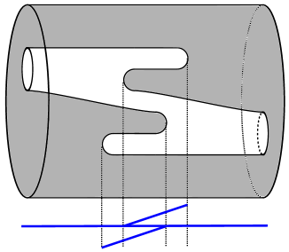
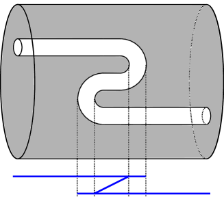
Figure 3. Spacetime representations of two mobile sensor networks. Covered regions are gray and uncovered regions are white. Each Reeb graph of the projection map $\pi$ from the uncovered region $\mathcal{U}$ to time $I$ appears in blue underneath the spacetime representation.

Formally, we define the Reeb graph as follows. Define an equivalence relation on $\mathcal{U}$ by declaring $(x,t)\sim(x^{\prime},t)$ whenever $x$ and $x^{\prime}$ belong to the same connected component of $\pi^{-1}(t)$. In particular, if $t\neq t^{\prime}$ then necessarily $(x,t)\not\sim(x^{\prime},t^{\prime})$. The Reeb graph of $\pi$ is the quotient space $\mathcal{U}/\sim$. See Figure 3 for examples.

In a mobile sensor network, each boundary cycle of the 1-skeleton of the alpha complex at time $t$ corresponds either to a connected component of the uncovered region $U(t)$, or alternatively to a 2-simplex of the alpha complex (i.e. a region of space covered by sensing domains). In solving Problems 3.2 and 3.3, we will track the boundary cycles as they are born, split, merge, and die. We will maintain labels on boundary cycles over time, encoding whether or not they may contain an intruder. Intruders can never be present in a boundary cycle corresponding to a 2-simplex, and they may or may not be present in other boundary cycles depending on the time-evolution of the network. By tracking the boundary cycles, we will actually be tracking the connected components of $U(t)$ as time $t$ varies. The algorithms presented in this paper are thus equivalent to computing the Reeb graph of $\pi$.

4. Algorithm for mobile coverage

The algorithm we present is based on [3, Theorem 3], which states that the time-varying alpha complex and time-varying rotation information are sufficient to determine whether or not an evasion path exists in a connected mobile sensor network. While making this theorem algorithmic, one of our key contributions is to present an implementation which is not state-based.

The structures used in [3, Theorem 3] are presented in an ad-hoc way; what is the intuition behind using the alpha complex and rotation data? The intuition comes from [3, Figure 13], which shows the time-varying connectivity data in a sensor network alone cannot determine whether or not an evasion path exists. More information about how the covered region is embedded into spacetime is required. Since our sensors live in the plane, this extra embedding information can take the form of weak rotation data: each sensor measures the cyclic order of its neighboring sensors. Through the ideas presented in Section 3.3, we are able to obtain a combinatorial representation of the uncovered region’s components. We note that this rotation information distinguishes the two examples in [3, Figure 13].

It should be noted that in [3, Theorem 3] the authors assume the alpha complex remains connected. We will maintain this assumption; see Section 5 for more on relaxing this assumption.

The question of whether or not the time-varying Čech complex of a sensor network, in conjunction with rotation data, is enough to determine if an evasion path exists is unknown — see the open question on Page 13 of [3]. However, [3, Theorem 3] shows that the time-varying alpha complex is sufficient when equipped with rotation data. This result relies on the fact that the edges of an alpha complex form a planar graph whereas the edges of a Čech complex may not; see [3, Figure 14]. We can therefore use the rotation data to extract the boundary cycles of this planar graph. Some of these boundary cycles will correspond to a connected component of the complement of the covered region; the main idea is to maintain labels on all boundary cycles and record whether the enclosed region may contain an intruder or not. Indeed, these labels can be used to recover the Reeb graph, and thus determine whether or not an evasion path exists.

4.1. Discrete-time problem

So far, the evasion path problem, Reeb-graph, and time-varying alpha complex have all been continuously varying in time. We now discretize the problem so that we can track evasion paths in a time-stepping fashion. As mentioned above, the idea is to track regions where an intruder could exist and use this information to infer the existence of an evasion path. This is done discretely by splitting the time domain $I$ into discrete time-intervals $[t_{n},t_{n+1}]$, where $\Delta t=t_{n+1}-t_{n}$ is assumed to be sufficiently small. Then, we solve a discrete evasion path problem on $[t_{n},t_{n+1}]$ using only information from time $t_{n}$ and $t_{n+1}$. Formally, on each time-interval we solve the following discrete problem:

Problem 4.1.

Let $\mathcal{H}_{n}=\{p(t_{n})\in D~{}|~{}p\text{ is an evasion path on }D\times[0,t_{n}]\}$ be the region which may contain an intruder at time $t_{n}$. Determine the existence of an evasion path $p\colon[t_{n},t_{n+1}]\rightarrow D$ such that $p(t_{n})\in\mathcal{H}_{n}$.

Solving this problem on successive time-intervals allows us to determine the mobile coverage, and existence of evasion paths, independently from the time domain used. In particular, the end-time need not be known a priori. Indeed, the following can be seen via a simple inductive argument:

Lemma 4.2.

Solving Problem 4.1 iteratively produces a solution to the continuous evasion path Problem 3.2 and the discrete analog of Problem 3.3.

The idea in using an alpha complex on $X$ is to partition $D$ into regions which will be labelled as feasibly having an intruder or not. If a region is marked as having a possible intruder at times $t_{n}$ and $t_{n+1}$, then under some modest assumptions we can say there is an evasion path on $[t_{n},t_{n+1}]$; see Section 4.2. The key is to use local rotational information so each of these regions can be identified by a unique boundary cycle. In this manner, the outline of the algorithm is straightforward and is shown in Algorithm 1. Once the labelling has been determined at time $t_{n+1}$, we can solve the discrete evasion path problem by simply looking for any regions labelled as feasibly having an intruder. An evasion path will exist if any boundary cycle is marked as possibly having an intruder. In solving the discrete problem, we additionally compute all information necessary to proceed forward in time.

Input : Alpha complex $A_{n}$, boundary cycles $B_{n}$, sensing radius $R$, boundary cycle labelling $L_{n}\colon B_{n}\rightarrow\{0,1\}$ at $t_{n}$

Output : A mapping $L_{n+1}\colon B_{n+1}\rightarrow\{0,1\}$, indicating whether each boundary cycle at $t_{n+1}$ may contain an intruder

begin

       $X_{n+1}\leftarrow UpdateSensors()$;

       $A_{n+1}\leftarrow ComputeAlphaComplex(X_{n+1},R)$;

       $rot\_data\leftarrow ComputeRotationalData(X_{n+1})$;

       $B_{n+1}\leftarrow ComputeBoundaryCycles(A_{n+1},rot\_data)$;

       $L_{n+1}\leftarrow UpdateBoundaryCycleLabelling(B_{n},B_{n+1},A_{n},A_{n+1},L_{n})$;

       return $L_{n+1}$

end

Algorithm 1 Single Time Step

4.2. Combinatorial changes in the alpha complex

Since the alpha complex is homotopy equivalent to the union of sensor balls, the alpha complex can determine the statically covered region of a sensing network (for further details see [8], which instead uses the closely related Vietoris–Rips complex). Heuristically, this is because the alpha complex partitions the domain into discrete regions where regions that are covered can be identified with 2-simplices of the alpha complex. Now that we have discretized the problem temporally, we may talk about a discrete sequence of static alpha complexes, each giving a combinatorial representation of the topology of the covered region at time $t_{i}$. We will denote this sequence of alpha complexes as $A_{i}$. In particular, $A_{i}$ is the alpha complex on $X$ at time $t_{i}$; we will further denote the sets of 1- and 2-simplices of $A_{i}$ as $A^{1}_{i}$ and $A_{i}^{2}$, respectively. However, as noted in [3], additional information is needed to determine which uncovered regions may contain intruders. This additional information comes in the form of the rotational information from the fat graph of the 1-skeleton of the alpha complex. One feature of using the alpha complex on $X$ is that it, along with the fat graph, can be constructed from information which is local to each sensor; see Appendix A.

As stated in Problem 4.1, we need $\Delta t$ to be sufficiently small. The ideas presented in [3] require only one of a fixed list of combinatorial changes occurs at each point in time (see Section 4.3). In the discrete setting, we relax this assumption so that on a given time-interval $[t_{n},t_{n+1}]$ we assume that $A_{n}$ and $A_{n+1}$ differ by only one of these combinatorial changes. In general, we will assume that, for a given time interval, we can subdivide the interval into sufficiently small sub-intervals as just described. While one could attempt to choose a uniform $\Delta t$ that satisfies this “sufficiently small” assumption, we found this impractical as it requires a rather strong assumption about the sensor motion being used. Instead, if more than one of these “atomic” combinatorial changes occurs in a given time-interval, we can simply subdivide the interval into two sub-problems recursively. In particular, there is an evasion path on $[t_{n},t_{n}+\Delta t]$ if there is an evasion path on $[t_{n},t_{n}+\frac{\Delta t}{2}]$ and on $[t_{n}+\frac{\Delta t}{2},t_{n}+\Delta t]$. This is equivalent to preforming a binary search for the intervals with only one combinatorial change. An example pseudo-code for this process is shown in Algorithm 3.

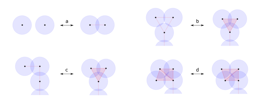
Figure 4. Atomic combinatorial changes within the alpha complex. (a) A single edge appears or disappears. (b) A single 2-simplex appears or disappears. (c) A 2-simplex and a free face edge simultaneously appear or disappear. (d) A Delaunay edge flip occurs.

Given the likely possibility that sensors move so the combinatorial change between $t_{n}$ and $t_{n+1}$ is not composed of a single atomic change, we proceed on the assumption that the sensors follow a model of motion for which, upon subdividing, we can find a time interval on which only one atomic change occurs. We note a shortcoming of this approach is we cannot detect changes that undo each other within a single time-step; however, this is inherent to the time discrete problem. For example, removing and then adding back the same edge within a single time-interval would be detected as no change in the alpha complex at all. This method of adaptive time-stepping also has the downside that a bulk of the computation needs to be preformed to determine if the adaptive step should be done. This can be quite costly, in a computational sense, as the number of sensors becomes large.

4.3. Tracking changes in boundary cycle labels

As described in the previous section, if we assume that the alpha complex remains connected, we may also assume there are only seven atomic combinatorial changes possible. Given that a combinatorial change occurred, we wish to (1) detect which type of combinatorial change occurred, (2) analyze the changes it will induce in the boundary cycles, and (3) determine how the associated boundary cycle labelling will change.

Suppose we know the alpha complexes at time $t_{n}$ and $t_{n+1}$, denoted $A_{n}$ and $A_{n+1}$. Additionally, assume the set of boundary cycles, $B_{n}$, are known at time $t_{n}$ with the associated labelling $L_{n}\colon B_{n}\rightarrow\{0,1\}$. We let $0$ denote that the corresponding cycle cannot contain an intruder, and $1$ denote that the corresponding cycle may contain an intruder. Given $A_{n+1}(X)$, we can compute the rotation data and obtain $B_{n+1}$. Now given this information as input, we want to determine which combinatorial change occurred, understand the associated changes in boundary cycles, and produce the appropriate boundary cycle labelling $L_{n+1}\colon B_{n+1}\rightarrow\{0,1\}$.

We can determine the transition that occurred by counting the number of boundary cycles, 1-simplices, and 2-simplices that are new and those that are no longer present. For example when an edge is added, this can be uniquely detected by verifying that $|A_{n+1}^{1}\setminus A_{n}^{1}|=1,\quad|A^{1}_{n}\setminus A^{1}_{n+1}|=0,\quad|A_{n+1}^{2}\setminus A_{n}^{2}|=0,\quad|A^{2}_{n}\setminus A^{2}_{n+1}|=0,|B_{n+1}\setminus B_{n}|=2,\quad|B_{n}\setminus B_{n+1}|=1$. A table for each atomic transition can be found in Table 1.

Table 1. The number of simplices and boundary cycles added or removed under atomic transitions.

	$|A_{n+1}^{1}\setminus A_{n}^{1}|$	$|A^{1}_{n}\setminus A^{1}_{n+1}|$	$|A_{n+1}^{2}\setminus A_{n}^{2}|$	$|A_{n}^{2}\setminus A_{n+1}^{2}|$	$|B_{n+1}\setminus B_{n}|$	$|B_{n}\setminus B_{n+1}|$
Add edge	1	0	0	0	2	1
Remove edge	0	1	0	0	1	2
Add 2-simplex	0	0	1	0	0	0
Remove 2-simplex	0	0	0	1	0	0
Add free edge and 2-simplex	1	0	1	0	2	1
Remove free edge and 2-simplex	0	1	0	1	1	2
Delaunay edge flip	1	1	2	2	2	2

We now analyze the changes in boundary cycles; see Figure 5 for illustrations of each atomic transition. We assume only the following transitions may occur:

• 1-simplex is added. When a 1-simplex is added, there will always be one old boundary cycle being split into two new boundary cycles. So the labelling of the two new boundary cycles will inherit the label of the old (removed) boundary cycle.

• 1-simplex is removed. When a 1-simplex is removed, we will always have two old boundary cycles joining together into one new boundary cycles. So the new boundary cycle will be labelled as potentially having an intruder if either of the old boundary cycles may have had an intruder.

• 2-simplex added. When a 2-simplex is added, once the corresponding boundary cycle is identified, it can be set as having no intruder.

• 2-simplex removed. When a 2-simplex is removed, the corresponding boundary cycle needs to be identified. This boundary cycle, which was previously labelled with no intruder, will maintain the same label.

• Pair consisting of a 2-simplex and a free edge is added. The label updating is similar to adding a 1-simplex but now, we must determine which boundary cycle corresponds to the new 2-simplex and set its label to have no intruder. This update can be achieved through the composition of adding a 1-simplex, and then adding the 2-simplex.

• Pair consisting of a 2-simplex and a free edge is removed. Just as in adding a simplex pair, the labelling for this case can be done by removing the 1-simplex and then removing the 2-simplex.

• Delaunay edge flip. A Deluanay edge flip occurs when the two triangles filling in a quadrilateral flip; see Figure 4d. The new boundary cycles will be labelled false since they are 2-simplices.

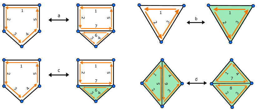
Figure 5. Atomic boundary cycle updates. These updates correspond to the atomic combinatorial changes within the alpha complex illustrated in Figure 4.

While [19] treats the boundary cycle label update as a state-based algorithm, we observe that this is not necessary. This was initially surprising to us, given that the proof of [3, Theorem 3] is heavily reliant on its case-based organization. Indeed, the aforementioned updates on the boundary cycles, to produce $L_{n+1}$ from $L_{n}$, simultaneously works for all of the atomic changes shown in Figure 5. This comes from the realization that we can simply add/remove the 1-simplex (if applicable) and then label all 2-simplices as having no intruder. This is put into pseudo-code in Algorithm 2.

Input : Alpha complex $A_{n+1}$, the boundary cycles $B_{n}$ and $B_{n+1}$, boundary cycle labelling $L_{n}\colon B_{n}\rightarrow\{0,1\}$

Output : The mapping $L_{n+1}\colon B_{n+1}\rightarrow\{0,1\}$, indicating whether each boundary cycle may contain an intruder

begin

       for $b\in B_{n}\cap B_{n+1}$ do

             $L_{n+1}[b]\leftarrow$ $L_{n}[b]$;

            

       end for

      for $b\in B_{n+1}\setminus B_{n}$ do

             $L_{n+1}[b]\leftarrow\bigvee\limits_{x\in B_{n}\setminus B_{n+1}}L_{n}[x]$;

            

       end for

      for $b\in B_{n+1}$ do

             if Nodes of $b$ form a 2-simplex then

                   $L_{n+1}[b]\leftarrow\mathbf{False}$;

                  

             end if

            

       end for

      

      return $L_{n+1}$;

      

end

Algorithm 2 Labelling Update - Serialized

5. Extension to disconnected sensor networks

In Section 4.3, we operate entirely under the assumption that the sensor network, or equivalently the alpha complex, remains connected. If we wish to investigate arbitrary models of motion, we need to allow the sensor network to become disconnected. However, the algorithm from Section 4 does not work in the context of disconnected sensor networks, as explained in Figure 16 of [3]. Indeed, it shows two sensor networks — both of which become disconnected — which have the same alpha complex and rotation information, yet one contains an evasion path while the other does not. We now present a modification of the evasion path problem that allows us to determine existence of evasion paths without this rather restrictive assumption of the sensors maintaining connectivity.

In our setup, the boundary senors are immobile and only the the interior sensors move in some prescribed motion. The main idea is to ignore sensors that become disconnected from the fence component until they are reconnected, in a similar model to that considered in [8]. This can be physically motivated by considering the scenario where disconnected sensors are out of range of the main computing network, or alternatively, we can imagine a setup where sensors that are disconnected from the fence are disconnected from a power source. For this reason we will refer to this model of allowing disconnected sensors as the “power-down model;” analogously, any algorithm which solves Problem 3.2 and allows disconnected sensors to remain turned on will be referred to as a “power-on model.”

Topologically, this modification changes the definition of the covered region as follows. Recall that $F\subset X$ is the subset of fence sensors. At each time $t$, we partition the covered region $C(t)=\cup_{x\in X}B_{r}(x(t))$ into two regions: the part that is in the same connected component as the fence sensors, and the part that is not in this connected component. This partitions the set $X$ of sensors into two groups: $X=X^{\prime}\coprod X^{\prime\prime}$, where $X^{\prime}\supseteq F$ is the set of sensors in the same connected component of $C(t)$ as the fence sensors, and where $X^{\prime\prime}=X\setminus X^{\prime}$ is the set of sensors which are not in this component. In the power-down model, all of the sensors in $X^{\prime\prime}$ are turned off, and do not contribute to the covered region. Indeed, the covered region in the power-down model is $\tilde{C}(t)=\cup_{x\in X^{\prime}(t)}B_{r}(x(t))$. We are still interested in whether or not there exists an evasion path, i.e. a continuous path $p\colon I\to D$ with $p(t)\notin\tilde{C}(t)$ for all times $t$. With this modified notion of an evasion path, we can proceed with solving Problem 3.2.

We remark that our algorithm for detecting mobile coverage with possibly disconnected sensor networks in the power-down model is still local, relying only on alpha complexes (which can be computed locally as explained in Appendix A) and weak rotation data. As shown in Figure 16 of [3], no locally based algorithm can exist with a “power-on” model (in which disconnected sensors remain on); any such algorithm would be inherently non-local. Nevertheless, our local algorithm for the power-down model still gives one-sided bounds for the power-on model: if no evasion path exists with the power-down sensors, then no evasion path exists for power-on sensors undergoing the same motions. Similarly, if an evasion path $p$ exists for the power-on model, then $p$ is also an evasion path for the power-down model. These are consequences of the inclusion $\tilde{C}(t)\subseteq C(t)$ of the covered regions in the two different models, for all $t$.

An attractive feature of the power-down modification is that it adds no complexity or data structures to existing code. In the context of the previous sections, the only modification is that we allow for two additional atomic combinatorial changes corresponding to components becoming connected or disconnected from the fence. We additionally can ignore all transitions that occur within a disconnected component.

We follow the same time discretization process as in Section 4; the only difference is that we must handle the additional cases where components of the alpha complex become disconnected or reconnected. This is a only a minor modification thanks to the following observation:

Lemma 5.1.

Under the assumption that at most one combinatorial change listed in Section 4.3 happens within each time-step, then a component of the alpha complex can only become disconnected (or reconnected) if a single edge is removed (or added) to the alpha complex.

5.1. Boundary cycle label updates

When a component of the alpha complex becomes disconnected from the fence, we will have a single boundary cycle initially surrounding a hole which will then be split into two boundary cycles; see Figure 6 for illustration. One of these boundary cycles will correspond to the outside of a new disconnected component; it will not be given any label. The other will be a hole enclosing the disconnected component and will be connected to the fence; we will maintain a label for this boundary cycle, and its initial label will be the same as the prior boundary cycle that split. In later time steps, any boundary cycle on a disconnected component will not be labeled. This represents the idea that the sensors that become disconnected are not a part of the power-down alpha complex. This atomic change can be detected just as in Section 4.3; see Table 2.

When a disconnected component becomes reattached to the fence through the addition of a 1-simplex, we will have the two previously described boundary cycles merging into one. All of the newly connected boundary cycles will be labeled to match the outer enclosing boundary cycle; however, any 2-simplices will be labeled as having no intruder. Again, this atomic change can be detected by simply counting the number of boundary cycles and simplices in the alpha complex before and after the transition; see Table 2.

We can detect if a component has become disconnected or reconnected by simply extending Table 1 with the following two cases.

Table 2. The number of simplices and boundary cycles added or removed under the additional possible atomic transitions (extending Table 1) in the power-down model.

	$|A_{n+1}^{1}\setminus A_{n}^{1}|$	$|A^{1}_{n}\setminus A^{1}_{n+1}|$	$|A_{n+1}^{2}\setminus A_{n}^{2}|$	$|A_{n}^{2}\setminus A_{n+1}^{2}|$	$|B_{n+1}\setminus B_{n}|$	$|B_{n}\setminus B_{n+1}|$
Disconnect	0	1	0	0	2	1
Reconnect	1	0	0	0	1	2

Figure 6. A component of the alpha complex disconnects from the fence component. From left to right, a single edge disappears, producing an additional connected component. From right to left, a single edge appears, merging two connected components into one.

6. Detection time statistics for diffusive sensors

We compute and examine the detection time $T_{\max}$ distributions assuming the mobile sensors move diffusively. Indeed, diffusion is relevant when minimal sensor networks experience random environmental forces, such as winds.

In all of the models of sensor motion we consider (diffusion, billiards, and collective motion), the initial locations of the sensors at time zero are chosen uniformly at random inside the domain.

6.1. Domain geometry

Our domain is $D=(1+\delta)S$, where $S$ is the unit square centered at the origin and $\delta>0$ is small and fixed. The sensing domains of the immobile fence sensors cover the boundary $\partial D$. We require that the mobile sensors remain within the unit square $S$. In particular, mobile sensors reflect elastically off of the boundary of $S$. We initialize the locations of the mobile sensors by placing them uniformly at random within $S$.

6.2. Performance of Brownian mobile sensor networks

We assume that each mobile sensor moves independently and satisfies the stochastic differential equation

$$\mathrm{d}\bm{x}_{t}=f(\bm{x}_{t})\,\mathrm{d}t+\sigma\,\mathrm{d}\bm{W}_{t},$$

where $\bm{W}_{t}$ denotes standard two-dimensional Brownian motion. We examine $T_{\max}$ statistics assuming no drift ($f$ vanishes), upon varying both the sensing radius $r$ and the number of mobile sensors $N$. We generated $T_{\max}$ distributions by performing 500 mobile sensor network simulations for each $(N,r)$ pair and using our algorithms to compute $T_{\max}$ for each simulation. We used diffusion coefficient $\sigma=0.5$ for every simulation.

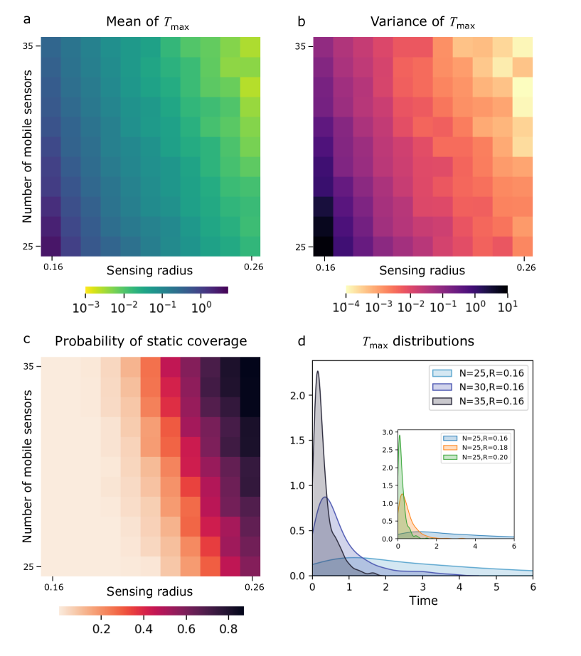
Figure 7. Detection time statistics for Brownian mobile sensor networks. The heatmaps illustrate (a) mean detection time $E[T_{\max}]$, (b) detection time variance $\operatorname{Var}[T_{\max}]$, and (c) the probability that the union of the sensing balls covers the entire domain $D$ at time $t=0$. We vary the sensing radius $r$ and the number $N$ of mobile sensors. (d) Detection time distributions for various $(N,r)$ pairs.

Figure 7d illustrates several of these distributions. Notice that they are unimodal. Further, the $T_{\max}$ distribution concentrates near $t=0$ as $N$ increases (for fixed $r$) and as $r$ increases (for fixed $N$). The probability that the sensing balls collectively cover the entire domain $D$ at time $t=0$ (that is, the probability of static coverage) varies widely over $(N,r)$-space (Figure 7c). Importantly, even when the probability of static coverage is low (Figure 7c, lower-left corner), the mobile sensor network nevertheless detects all possible evaders relatively quickly (Figure 7a, lower-left corner).

As expected, Figure 7a indicates that $E[T_{\max}]$ decreases as $r$ increases (for fixed $N$) and as $N$ increases (for fixed $r$). For Brownian mobile sensor networks, $\operatorname{Var}[T_{\max}]$ behaves the same way (Figure 7b). As we will see, detection time variances can behave quite differently if the mobile sensors locally coordinate motion.

7. Collective motion improves mobile sensor network performance

Suppose the mobile sensors are capable of self-propulsion. How should the mobile sensors move in order to optimize performance of the sensor network? Suppose that each mobile sensor can compute the relative positions of nearby sensors. Can improved mobile sensor network performance emerge when the mobile sensors use this local position data to locally coordinate?

We answer this question affirmatively by allowing the mobile sensors to use attractive and repulsive forces for local coordination. In particular, we use the D’Orsogna model [11], a seminal effort to explain the emergent phenomena that arise when agents move collectively. We compare this ‘locally strategic’ model to a ‘locally oblivious’ alternative wherein the mobile sensors move independently as simple billiard particles.

7.1. Billiard motion

Our domain geometry is as in Section 6.1. We initialize the sensor network by randomly placing each of the $N$ mobile sensors uniformly at random within the unit square $S$ and assigning each a random initial direction of motion $\theta_{k}\in\mathbb{R}/2\pi\mathbb{Z}$. Each mobile sensor moves independently of the others at unit speed and changes direction of motion only when colliding elastically with the virtual boundary $\partial S$.

7.2. Collective mobile sensor motion

The D’Orsogna model uses attractive and repulsive potentials to model the dynamics of animal collectives such as fish schools and bird flocks. Here, we show that if mobile sensors use such potentials to locally coordinate, the emergent collective motion can cause these D’Orsogna sensor networks to outperform billiard sensor networks.

The $N$ mobile sensors $\bm{x}_{k}$ obey the nonlinear system

(1a) $$\frac{\mathrm{d}\bm{x}_{k}}{\mathrm{d}t} =\bm{v}_{k}$$

(1b) $$\mathfrak{m}\frac{\mathrm{d}\bm{v}_{k}}{\mathrm{d}t} =(\alpha-\beta\|\bm{v}_{k}\|^{2})\bm{v}_{k}-\sum_{\begin{subarray}{c}m=1\\ m\neq k\end{subarray}}^{N}g(\|\bm{x}_{m}-\bm{x}_{k}\|)\nabla_{k}U_{m}(\bm{x}_{k}).$$

The generalized Morse potential

(2) $$U_{m}(\bm{x}_{k})=C_{r}e^{-\|\bm{x}_{m}-\bm{x}_{k}\|/\ell_{r}}-C_{a}e^{-\|\bm{x}_{m}-\bm{x}_{k}\|/\ell_{a}}$$

describes the interaction between sensors $m$ and $k$. The parameters $\ell_{a}$ and $\ell_{r}$ in Eq. (2) quantify the length scales for attraction and repulsion, respectively. The parameters $C_{a}$ and $C_{r}$ quantify attraction and repulsion magnitudes.

The function $g$ localizes the interaction force to ensure that sensors $m$ and $k$ only interact if they are near one another. Our use of the localizer $g$ is consistent with our minimal sensing approach: The mobile D’Orsogna sensors should only have the ability to gather and react to local conditions. Concretely, $g$ is given by

$$g(x)=\begin{cases}1,&\text{if }x<2r,\\ 0,&\text{if }x\geqslant 2r.\end{cases}$$

We note that two sensors interact, affecting each other’s motion, if and only if their sensing balls of radius $r$ overlap.

In isolation, mobile D’Orsogna sensor $k$ only feels the force $(\alpha-\beta\|\bm{v}_{k}\|^{2})\bm{v}_{k}$ and will therefore approach the asymptotic speed $\sqrt{\alpha/\beta}$. In equilibrium, speeds of the mobile D’Orsogna sensors should statistically fluctuate about this asymptotic value.

7.3. Parameter selection for model comparison

The mobile billiard sensors move at unit speed. We have set $\alpha=\beta=1$ in Eq. (1b) so that the equilibrium speeds of the mobile D’Orsogna sensors fluctuate about one. This choice matches the characteristic speeds of the two models, allowing for a meaningful sensor network performance comparison.

We have set the attraction and repulsion length scales in the D’Orsogna potential (2) to $\ell_{a}=1$ and $\ell_{r}=0.1$, respectively. The scale separation here models collective animal behavior, namely short-range repulsion, and attraction over longer distances. We have set the attraction and repulsion magnitude parameters to $C_{a}=0.45$ and $C_{r}=0.5$, respectively. The mobile D’Orsogna sensors have mass $\mathfrak{m}=1$.

7.4. D’Orsogna sensor networks outperform billiard sensor networks

We computed detection time $T_{\max}$ distributions for both the D’Orsogna sensor network and the billiard sensor network. We did so by performing 500 simulations for each choice of sensing radius $r$ and number of mobile sensors $N$. Figure 8 compares $E[T_{\max}]$ and $\operatorname{Var}[T_{\max}]$ behavior for the two sensor network models.

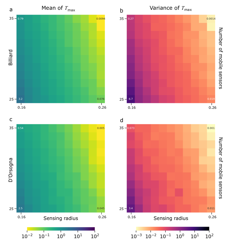
Figure 8. Performance comparison of D’Orsogna and billiard mobile sensor networks. Heatmaps illustrate detection time statistics as functions of the sensing radius $r$ and the number of mobile sensors $N$. Left column: Mean detection time. Right column: Detection time variance. Top row: Billiard sensor network. Bottom row: D’Orsogna sensor network.

Importantly, the D’Orsogna network detects evaders more quickly on average than the billiard network (Figure 8ac). Quantitatively, averaging

$$\frac{E[T_{\max}](\text{billiard})-E[T_{\max}](\text{D'Orsogna})}{E[T_{\max}](\text{billiard})}$$

over all $(N,r)$ pairs, we find that the D’Orsogna network outperforms the billiard network by $23.5\%$.

As is the case for the Brownian network, $\operatorname{Var}[T_{\max}]$ varies monotonically with $r$ and with $N$ for the billiard network (Figure 8b) and the D’Orsogna network (Figure 8d).

8. Conclusion

Minimal sensor networks attempt to solve global sensing problems using local data. Assuming mobile planar sensors collect local connectivity data, local distance data, and weak rotation information, can we determine whether or not an evasion path exists? Adams and Carlsson answer this question affirmatively [3, Theorem 3]. Here, we have converted this theorem into explicit algorithms that allow us to compute detection time distributions for both deterministic and stochastic mobile sensor networks. We have computed and analyzed these distributions for sensor networks with Brownian, billiard, and D’Orsogna motion models. Comparing the two deterministic mobile networks, the D’Orsogna system outperforms its billiard counterpart. This suggests that emergent dynamics resulting from collective local motion can positively impact mobile sensor network performance.

We end with open questions and potential areas for future research. Opportunities exist for both theoretical and computational investigations.

1. The expected time to achieve mobile coverage decreases as we increase the number of sensors or as we increase the sensing radius. Do phase transition phenomena ever arise?

2. In the limit as the number of sensors goes to infinity and the sensing radius of each sensor goes to zero, can one describe the asymptotics of the expected time to achieve mobile coverage? Does the distribution of this detection time, $T_{\max}$, converge in this limit? If it does, to what limiting distribution? How do these asymptotics depend on the model of sensor motion?

3. For deterministic sensor motion models, how do the statistics of $T_{\max}$ depend on the underlying invariant measure and rate of decay of correlations?

4. The detection time distributions in Figure 7d are unimodal. Is this always the case for Brownian motion? What happens for different models of motion?

5. What collective motion models, wherein each mobile sensor can adjust its motion based on the relative positions of its local (but not global) neighbors, are the most effective at decreasing the expected time until mobile coverage is achieved?

6. What can be said about collections of sensors with randomly varying sensing radii?

7. What do the statistics for mobile coverage look like in the power-on model, wherein mobile sensors are allowed to become disconnected but still all remain on?

8. How do the statistics for mobile coverage change as the domain varies? For instance, what happens on a torus, or on other domains that are not simply connected?

9. How would the presence of hyperbolicity in the dynamics impact mobile sensor network performance? For instance, what happens if the mobile sensors move as billiard particles and reflect off of convex scatters (the Lorenz gas or Sinai billiard setup)?

9. Acknowledgments

We would like to acknowledge Michael Kerber for showing us the result in Appendix A.

10. Funding

This work has been partially supported by National Science Foundation grant DMS 1816315 (William Ott).

11. Code availability

See [1] for code and documentation.

Appendix A Local distances determine the alpha complex

Let $X=\{x_{1},x_{2},\ldots,x_{n}\}\subset\mathbb{R}^{m}$ be a collection of $n$ points in general position. Let $A(X,r)$ be the alpha complex on $X$ with radius parameter $r>0$, as defined in Section 3.2 for the particular case $m=2$. The following proposition says that if one knows only the local distances between points in $X$ (those distances between points whose closed balls of radius $r$ overlap), then this knowledge is sufficient to compute the alpha complex $A(X,r)$.

Proposition A.1.

Suppose that for each $i,j\in\{1,\ldots,n\}$ we know

• whether or not $\|x_{i}-x_{j}\|\leq 2r$, and

• the value of $\|x_{i}-x_{j}\|$ if $\|x_{i}-x_{j}\|\leq 2r$.

Then we can determine $A(X,r)$.

To prove this claim we need some definitions and a lemma from [18] (see also [6] for related ideas). Let $\sigma$ be a $k$-simplex with vertices in $X$. Due to our general position assumption, there is a unique $(k-1)$-dimensional sphere in the $k$-plane containing $\sigma$ that circumscribes $\sigma$. Let the center and radius of this sphere be the circumcenter and circumradius of $\sigma$. Let the $m$-dimensional ball with this center and radius be the circumball of $\sigma$.

Definition A.2.

Simplex $\sigma$ is short if its circumradius is at most $r$.

Definition A.3.

Simplex $\sigma$ is Gabriel if its circumball has no point of $X$ in its interior.

Lemma A.4 ([18]).

Simplex $\sigma$ is in $A(X,r)$ if and only if it is

• short and Gabriel, or

• the face of a simplex that is short and Gabriel.

We would like to thank Michael Kerber for showing us the following proof.

Proof of Proposition A.1.

Let $\sigma$ be a $k$-simplex with with vertices in $X$. By Lemma A.4 it suffices to determine if $\sigma$ is short and Gabriel, because $A(X,r)$ is the collection of all such simplices and their faces.

If the distance between any two vertices of $\sigma$ is more than $2r$, then $\sigma$ is not short. Hence we assume that all pairwise distances between vertices of $\sigma$ are at most $2r$, and so we know these distances exactly. We thus know the shape of $\sigma$ up to a rigid motion of $\mathbb{R}^{m}$. This allows us to determine the circumcenter and circumradius of $\sigma$. Simplex $\sigma$ is short if its circumradius is at most $r$.

Next we must determine if $\sigma$ is Gabriel. Let $x$ be a point in $X$ that is not a vertex of $\sigma$; we must decide if $x$ is in the circumball of $\sigma$. If the distance between $x$ and any vertex of $\sigma$ is more that $2r$, then $x$ is not in the circumball of $\sigma$ because the circumball has radius at most $r$. Hence we assume that the distance between $x$ and each vertex of $\sigma$ is at most $2r$, and so we know these distances exactly. We thus know the shape of $\sigma\cup\{x\}$ up to a rigid motion of $\mathbb{R}^{m}$. This allows us to determine if $x$ is in the circumball of $\sigma$, and hence if $\sigma$ is Gabriel. ∎

Appendix B Pseudocode

This appendix contains pseudocode for algorithms referenced throughout the paper. Algorithm 3 shows how the timestepping can be preformed in an adaptive manner to ensure that only one atomic combinatorial change happens at a time. Algorithm 4 shows a case-based algorithm, to be contrasted with the non-case-based (and much shorter) Algorithm 2. Finally, Algorithm 5 shows how the assumption that the alpha complex remain connected may be relaxed while updating labels for the boundary cycles in the power-down model.

Input : Sensor positions $X_{n}$, alpha complex $A_{n}$, the boundary cycles $B_{n}$, boundary cycle labelling $L_{n}\colon B_{n}\rightarrow\{0,1\}$, current time $t$, timestep size $\Delta t$, sensing radius $R$

Output : Sensor positions $X_{n+1}$, alpha complex $A_{n+1}$, the boundary cycles $B_{n+1}$, boundary cycle labelling $L_{n+1}\colon B_{n}\rightarrow\{0,1\}$

begin

       $X_{n+1}^{*}\leftarrow UpdatePositions(X_{n},dt)$;

       $A_{n+1}^{*}\leftarrow AlphaComplex(X_{n}^{*},R)$;

       $B_{n+1}^{*}\leftarrow ComputeBoundaryCycles(A_{n}^{*},X_{n}^{*})$;

       Remove boundary cycle corresponding to fence from $B_{n+1}^{*}$;

       if Atomic Transition occurred then

             $L_{n+1}\leftarrow LabelUpdate(B_{n},B_{n}^{*},A_{n}^{*},L_{n})$ via Algorithm 2 or 5;

             return $X_{n+1}^{*},A_{n+1}^{*},B_{n+1}^{*},L_{n+1}$

      else

             $X_{n+\frac{1}{2}},A_{n+\frac{1}{2}},B_{n+\frac{1}{2}},L_{n+\frac{1}{2}}\leftarrow AdaptiveTimeStep(\frac{\Delta t}{2},t,R,X_{n},A_{n},B_{n},L_{n})$;

             $X_{n+1},A_{n+1},B_{n+1},L_{n+1}\leftarrow AdaptiveTimeStep(\frac{\Delta t}{2},t+\frac{\Delta t}{2},R,X_{n+\frac{1}{2}},A_{n+\frac{1}{2}},B_{n+\frac{1}{2}},L_{n+\frac{1}{2}})$;

             return $X_{n+1},A_{n+1},B_{n+1},L_{n+1}$

       end if

      

end

Algorithm 3 Single Adaptive Time-Step

Input : Alpha complex $A_{n+1}$, the boundary cycles $B_{n}$ and $B_{n+1}$, boundary cycle labelling $L_{n}\colon B_{n}\rightarrow\{0,1\}$, fence sensors $F$

Output : The mapping $L_{n+1}\colon B_{n+1}\rightarrow\{0,1\}$, indicating whether each boundary cycle may contain an intruder

begin

       for $b\in B_{n}\cap B_{n+1}$ do

             $L_{n+1}\leftarrow L_{n}$;

            

       end for

      switch Atomic transition do

             case 1-Simplex is added do

                   $x\leftarrow$ only cycle in $B_{n}\setminus B_{n+1}$ ;

                   for $b\in B_{n+1}\setminus B_{n}$ do

                         $L_{n+1}[b]\leftarrow L_{n+1}[x]$;

                        

                   end for

                  

             end case

            case 1-Simplex is removed do

                   $b\leftarrow$ only cycle in $B_{n+1}\setminus B_{n}$ ;

                   $L_{n+1}[b]\leftarrow\bigvee\limits_{x\in B_{n}\setminus B_{n+1}}L_{n}[x]$;

                  

             end case

            case 2-Simplex is added do

                   $b\leftarrow$ boundary cycle associated with new simplex;

                   $L_{n+1}[b]\leftarrow$ False ;

                  

             end case

            case 2-Simplex is removed do

                   continue ;

                  

             end case

            case Simplex pair added do

                   $x\leftarrow$ only cycle in $B_{n}\setminus B_{n+1}$ ;

                   for $b\in B_{n+1}\setminus B_{n}$ do

                         if Nodes of $b$ form a 2-Simplex then

                               $L_{n+1}[b]\leftarrow\textnormal{{False}}$;

                              

                        else

                               $L_{n+1}[b]\leftarrow L_{n+1}[x]$;

                              

                         end if

                        

                   end for

                  

             end case

            case Simplex pair removed do

                   $b\leftarrow$ only cycle in $B_{n+1}\setminus B_{n}$ ;

                   $L_{n+1}[b]\leftarrow\bigvee\limits_{x\in B_{n}\setminus B_{n+1}}L_{n+1}[x]$;

                  

             end case

            case Delaunay edge flip do

                   for $b\in B_{n+1}\setminus B_{n}$ do

                         $L_{n+1}[b]\leftarrow\textnormal{{False}}$;

                        

                   end for

                  

             end case

            

       end switch

      for $b\in B_{n}\setminus B_{n+1}$ do

             $L_{n+1}[b]\leftarrow NULL$;

            

       end for

      return $L_{n+1}$;

      

end

Algorithm 4 Update Labelling

Input : Alpha complex $A_{n+1}$, the boundary cycles $B_{n}$ and $B_{n+1}$, boundary cycle labelling $L_{n}\colon B_{n}\rightarrow\{0,1\}$, fence sensors $F$

Output : The mapping $L_{n+1}\colon B_{n+1}\rightarrow\{0,1\}$, indicating whether each boundary cycle may contain an intruder

begin

       for $b\in\{y\in B_{n+1}\cap B_{n}\mid\text{nodes of y are connected to fence}\}$ do

             $L_{n+1}[b]=L_{n}[b]$;

       end for

       switch Atomic transition do

             case 1-simplex added causing re-connection do

                   $V=\{b\in B_{n}\setminus B_{n+1}\mid b\text{ is connected to }F\}$;

                   for $b\in B_{n+1}$ do

                         if  $b\text{ is connected to }F\text{ but has no label in }L_{n}$ then

                               $L_{n+1}[b]\leftarrow\bigvee\limits_{x\in V}L_{n}[x]$;

                              

                         end if

                        else if $b\text{ is connected to }F$  then

                               $L_{n+1}[b]\leftarrow L_{n}[b]$;

                              

                         end if

                        

                   end for

                  

             end case

            case 1-simplex removed causing disconnection do

                   $V=\{b\in B_{n+1}\mid\;b\text{ is not connected to }F\text{ but has label in }L_{n}\}$;

                   for $b\in B_{n+1}\setminus B_{n}$ do

                         if $b\text{ is connected to }F$ then

                               $L_{n+1}[b]\leftarrow\bigvee\limits_{x\in V}L_{n}[x]\vee L_{n}[b]$;

                              

                         end if

                        

                   end for

                  

             end case

            otherwise do

                   for $b\in B_{n+1}\setminus B_{n}$ do

                         if $b\text{ is connected to }F$ then

                               $L_{n+1}[b]\leftarrow\bigvee\limits_{x\in B_{n}\setminus B_{n+1}}L_{n}[x]$;

                              

                         end if

                        

                   end for

                  

             end case

            

       end switch

      for $b\in B_{n+1}$ do

             if Nodes of $b$ form a 2-Simplex and are connected to $F$ then

                   $L_{n+1}[b]\leftarrow\mathbf{False}$;

                  

             end if

            

       end for

      

      return $L_{n+1}$;

      

end

Algorithm 5 Update Labelling with Disconnected Components

References

- [1] https://github.com/elykwilliams/EvasionPaths.
- [2] H. Adams, Evasion paths in mobile sensor networks, PhD thesis, Stanford University, 2013.
- [3] H. Adams and G. Carlsson, Evasion paths in mobile sensor networks, International Journal of Robotics Research, 34 (2015), pp. 90–104, https://doi.org/10.1177/0278364914548051.
- [4] G. Carlsson and B. Filippenko, The space of sections of a smooth function, 2020, https://arxiv.org/abs/2006.12023.
- [5] J.-C. Chin, Y. Dong, W.-K. Hon, C.-T. Ma, and D. Yau, Detection of intelligent mobile target in a mobile sensor network, IEEE/ACM Transactions on Networking, 18 (2010), pp. 41–52, https://doi.org/10.1109/TNET.2009.2024309.
- [6] H. Chintakunta and H. Krim, Distributed boundary tracking using alpha and Delaunay–Čech shapes, arXiv preprint arXiv:1302.3982, (2013).
- [7] T. Chung, G. Hollinger, and V. Isler, Search and pursuit-evasion in mobile robotics A survey, Autonomous Robots, 31 (2011), pp. 299–316, https://doi.org/10.1007/s10514-011-9241-4.
- [8] V. De Silva and R. Ghrist, Coordinate-free coverage in sensor networks with controlled boundaries via homology, International Journal of Robotics Research, 25 (2006), pp. 1205–1222, https://doi.org/10.1177/0278364906072252.
- [9] V. de Silva and R. Ghrist, Coverage in sensor networks via persistent homology, Algebraic and Geometric Topology, 7 (2007), pp. 339–358, https://doi.org/10.2140/agt.2007.7.339.
- [10] V. De Silva and R. Ghrist, Homological sensor networks, Notices of the American Mathematical Society, 54 (2007), pp. 10–17.
- [11] M. D’Orsogna, Y. Chuang, A. Bertozzi, and L. Chayes, Self-propelled particles with soft-core interactions: Patterns, stability, and collapse, Physical Review Letters, 96 (2006), https://doi.org/10.1103/PhysRevLett.96.104302.
- [12] J. Gamble, H. Chintakunta, and H. Krim, Applied topology in static and dynamic sensor networks, 2012, https://doi.org/10.1109/SPCOM.2012.6290237.
- [13] R. Ghrist and S. Krishnan, Positive Alexander duality for pursuit and evasion, SIAM Journal on Applied Algebra and Geometry, 1 (2017), pp. 308–327, https://doi.org/10.1137/16M1089083.
- [14] P. Hall, Introduction to the theory of coverage processes, Wiley Series in Probability and Mathematical Statistics: Probability and Mathematical Statistics, John Wiley & Sons, Inc., New York, 1988, https://doi.org/10.1016/0167-0115(88)90159-0.
- [15] A. Hatcher, Algebraic Topology, Cambridge University Press, Cambridge, 2002.
- [16] K. Igusa, Higher Franz-Reidemeister torsion, vol. 31 of AMS/IP Studies in Advanced Mathematics, American Mathematical Society, Providence, RI; International Press, Somerville, MA, 2002, https://doi.org/10.1016/s0550-3213(02)00739-3.
- [17] A. M. Kellerer, On the number of clumps resulting from the overlap of randomly placed figures in a plane, J. Appl. Probab., 20 (1983), pp. 126–135, https://doi.org/10.2307/3213726.
- [18] M. Kerber and H. Edelsbrunner, 3d kinetic alpha complexes and their implementation, in 2013 Proceedings of the Fifteenth Workshop on Algorithm Engineering and Experiments (ALENEX), SIAM, 2013, pp. 70–77.
- [19] D. Khryashchev, J. Chu, M. Vejdemo-Johansson, and P. Ji, A distributed approach to the evasion problem, Algorithms (Basel), 13 (2020), pp. Paper No. 149, 13, https://doi.org/10.3390/a13060149.
- [20] H. La and W. Sheng, Flocking control of a mobile sensor network to track and observe a moving target, 2009, pp. 3129–3134, https://doi.org/10.1109/ROBOT.2009.5152747.
- [21] B. Liu, P. Brass, O. Dousse, P. Nain, and D. Towsley, Mobility improves coverage of sensor networks, 2005, pp. 300–308, https://doi.org/10.1145/1062689.1062728.
- [22] B. Liu, O. Dousse, P. Nain, and D. Towsley, Dynamic coverage of mobile sensor networks, IEEE Transactions on Parallel and Distributed Systems, 24 (2013), pp. 301–311, https://doi.org/10.1109/TPDS.2012.141.
- [23] B. Mohar and C. Thomassen, Graphs on surfaces, Johns Hopkins Studies in the Mathematical Sciences, Johns Hopkins University Press, Baltimore, MD, 2001.
- [24] P. A. P. Moran, The volume occupied by normally distributed spheres, Acta Math., 133 (1974), pp. 273–286, https://doi.org/10.1007/BF02392147.
- [25] R. Olfati-Saber, Flocking for multi-agent dynamic systems: Algorithms and theory, IEEE Transactions on Automatic Control, 51 (2006), pp. 401–420, https://doi.org/10.1109/TAC.2005.864190.
- [26] R. Olfati-Saber, Distributed Kalman filtering for sensor networks, 2007, pp. 5492–5498, https://doi.org/10.1109/CDC.2007.4434303.
- [27] R. Olfati-Saber, J. Fax, and R. Murray, Consensus and cooperation in networked multi-agent systems, Proceedings of the IEEE, 95 (2007), pp. 215–233, https://doi.org/10.1109/JPROC.2006.887293.
- [28] R. Olfati-Saber and P. Jalalkamali, Coupled distributed estimation and control for mobile sensor networks, IEEE Transactions on Automatic Control, 57 (2012), pp. 2609–2614, https://doi.org/10.1109/TAC.2012.2190184.
- [29] Y. Qu, S. Xu, C. Song, Q. Ma, Y. Chu, and Y. Zou, Finite-time dynamic coverage for mobile sensor networks in unknown environments using neural networks, Journal of the Franklin Institute, 351 (2014), pp. 4838–4849, https://doi.org/10.1016/j.jfranklin.2014.05.011.
- [30] G. Schroeter, Distribution of number of point targets killed and higher moments of coverage of area targets, Naval research logistics quarterly, 31 (1984), pp. 373–385, https://doi.org/10.1002/nav.3800310304.
- [31] H. Su, X. Chen, M. Chen, and L. Wang, Distributed estimation and control for mobile sensor networks with coupling delays, ISA Transactions, 64 (2016), pp. 141–150, https://doi.org/10.1016/j.isatra.2016.04.025.
- [32] H. Su, Z. Li, and M. Chen, Distributed estimation and control for two-target tracking mobile sensor networks, Journal of the Franklin Institute, 354 (2017), pp. 2994–3007, https://doi.org/10.1016/j.jfranklin.2017.01.033.
- [33] W. Yuan, N. Ganganath, C.-T. Cheng, Q. Guo, and F. Lau, Temnothorax albipennis migration inspired semi-flocking control for mobile sensor networks, Chaos, 29 (2019), https://doi.org/10.1063/1.5093073.