Nested Sampling Methods

Abstract

Nested sampling (NS) computes parameter posterior distributions and makes Bayesian model comparison computationally feasible. Its strengths are the unsupervised navigation of complex, potentially multi-modal posteriors until a well-defined termination point. A systematic literature review of nested sampling algorithms and variants is presented. We focus on complete algorithms, including solutions to likelihood-restricted prior sampling, parallelisation, termination and diagnostics. The relation between number of live points, dimensionality and computational cost is studied for two complete algorithms. A new formulation of NS is presented, which casts the parameter space exploration as a search on a tree data structure. Previously published ways of obtaining robust error estimates and dynamic variations of the number of live points are presented as special cases of this formulation. A new online diagnostic test is presented based on previous insertion rank order work. The survey of nested sampling methods concludes with outlooks for future research.

1 Context

Nested Sampling (NS, Skilling, 2004) is a Monte Carlo algorithm for computing an integral over a model parameter space. In the context of Bayesian inference of analysing some data $D$, the integrand is the likelihood function $L(D|\theta)$, which is marginalised over the parameters $\theta$ according to the prior probability density $\pi(\theta)\,d\theta$, which gives a measure of the parameter space. Integrals over the posterior density $L(D|\theta)\times\pi(\theta)d\theta$ allow insightful statements about what model parameters regions are probable or improbable. The integral over the entire parameter space, $Z=\int L(D|\theta)\,\pi(\theta)d\theta$, is known as the marginal likelihood or Bayesian evidence. The Bayes factor is the ratio of marginalised likelihoods of two different models, $Z_{M1}/Z_{M2}$. Multiplied by the model prior odds, the resulting posterior odds can be interpreted as the relative evidence among these two models, given the observed data. Selecting models using the Bayes factor can be performed based on empirical scales (e.g., Jeffreys, 1998; Kass and Raftery, 1995) or calibrated on false decision rates (e.g., Veitch and Vecchio, 2008; Buchner, 2019). The computation of marginal likelihoods is thus generally important for science with parametric probabilistic models (Evans, 2007). In practice, the computation of posteriors and the integral is achieved with Monte Carlo algorithms.

Exploring, navigating and integrating these parameter spaces can exhibit the following challenges (classification in priv. comm. with F. Beaujeau):

• (P) Peculiar shapes such as non-ellipsoidal (e.g., from non-Gaussian profiles) and non-convex posterior contours (e.g., bananas).

• (M) Multiple, well-separated modes, when several peaks in the posterior with comparable probability exist. One can define these by contours forming non-connected sets.

• (D) High dimensionality (here: intermediate: $d\sim 10$, high: $d>30$). High-dimensional spaces incur the curse of dimensionality and geometric intuition breaks down.

• (I) High information gain makes the posterior a very small portion (e.g., $e^{-10000}$) of the prior volume, that needs to be identified. A useful measure of how much the likelihood updates the prior is the information gain: $H=\int\log\frac{\pi(\theta)}{L(D|\theta)\times\pi(\theta)}\pi\,d\theta$.

• (T) Phase transitions are surprising and abrupt changes of the accessible parameter space $X$ with increasing likelihood $L$, i.e., when $g=\frac{d\log L}{d\log X}$ is not an up-concave function (Skilling et al., 2006). A illustrating example is the spike-and-slab likelihood, where a Gaussian is summed with another, much wider, co-centred Gaussian ($\sigma_{2}^{2}\gg\sigma_{1}^{2}$). Between the centre and scales of order $\sigma_{1}$, $g$ decreases quadratically approximately as $-(x-\mu)^{2}/\sigma_{1}^{2}$, but then slows its decrease and becomes almost constant between $\sigma_{1}$ and $\sigma_{2}$, where the “spike” ($\sigma_{1}$) occupies a tiny region on top of the wide slab ($\sigma_{2}$). Therefore, the parameter space accessible at a given $L$ increases first very slowly with decreasing $\log L$, then extremely rapidly, analogous to the volume expansion of water as it is heated to water vapor (Skilling et al., 2006). Such phase transitions commonly occur when a subdominant model component becomes relevant after a dominant component is constrained, for example in mixture models. Likelihood plateaus can be considered extreme phase transitions.

Naturally, a given problem can exhibit any combination of these challenges.

Nested sampling (introduced in §3) addresses these challenges. It makes computing $Z$ practical for a wide variety of problems. Posterior samples are simultaneously computed by NS. Beyond the application to Bayesian inference, NS has been applied as a general integration algorithm (e.g., Murray et al., 2006; Pártay, Bartók and Csányi, 2010; Malakar and Knuth, 2011; Goggans, Henderson and Cao, 2014; Birge, Chang and Polson, 2012) and to compute entropies (Malakar and Knuth, 2011; Brewer, 2017).

2 Review methodology

This review presents NS methods developed over the last 15 years. We conducted a systematic literature review to find works on nested sampling. We used four sources: (1) Google Scholar was searched with the terms “nested sampling” (including quotes) in Sep 2017. Of the 6080 search results of which we consider the first 260 (ranked by relevance by Google Scholar). We excluded results on the unrelated nested sampling technique for soil measurements by removing publications by one author from the query -“PC Mahalanobis” and further manually removed results. (2) Google Scholar citations of Skilling’s original 2004 Nested Sampling paper were searched with the search query “nested sampling” in September 2017. This yielded 420 search results which we all considered. (3) The NASA Abstract Database System was initially searched with the query "nested sampling". This gave 1215 results, many of which are simple applications of nested sampling without methodological contributions, mostly from astrophysics. We thus limit our search to the arXiv classes (arxiv_class:"stat.*" OR arxiv_class:"math.*" OR arxiv_class:"physics.*"), where papers developing statistical methods and algorithms are (cross-)posted. This yields 78 results, all of which were considered. (4) Works previously known to the first author were also included. Out of those four queries we consider works with novel contributions to any aspect of nested sampling methods.

Some restrictions are necessary to focus the content. Firstly, we limit ourselves to inference problems over continuous parameter spaces. NS does not require the space to be continuous, only that a prior is defined from which can be sampled. The “objects” considered can be of categorical nature or of varying dimensionality (e.g., Brewer, 2014). Furthermore, the review does not go into depth on probability theoretical analyses of NS. This is mathematically involved and already covered elsewhere, to which we refer the interested reader in sections 3.2 and 4. We exclude works which merely apply nested sampling in a previously published form to a new problem without modifications of any aspect of an existing algorithm, and further exclude works which do not describe the specific method they use.

The review made clear that NS is developed in communities with limited communication. The first sections introduce NS from the view points of Bayesian practitioners (3.1), statisticians (3.2), physicists (3.3) and computer scientists (3.4). Using the language of each group these sections attempt to allow experts to exchange their ideas better. The focus of this review are techniques for implementing the components of NS, enumerated in section 3.5, in such a way that they efficiently address the PMDIT challenges. Section 4 gives an introduction to the integration procedure, and references convergence proofs. Termination criteria are discussed in §4.3, followed by a discussion of the computational complexity in §4.4. Diagnostics to determine the correctness and quality of a NS run are presented in §4.5, including a new test. Sampling methods for use inside NS are extensively reviewed, including methods based on random walks (§5.1), rejection sampling (§5.2), and hybrids (§5.3). Section 6 then discusses variations of NS, which soften the hard likelihood constraint, vary the number of live points and parallelise the algorithm. In §7, a simple numerical experiment demonstrates some of the behaviours of NS implementations.

The survey of techniques presented helped inform design decisions for our own open-source NS implementation. UltraNest is a high-performance general purpose nested sampling library for models written in the Python, C, C++, Fortran, Julia or R programming languages, with a focus on reliability. We document the design decisions for UltraNest in the relevant sections.

3 Introduction to Nested Sampling

We present introductions aimed at different audiences, with the goal of enabling different groups to translate between their languages used. The sections present an introduction NS from the perspective of a Bayesian practitioner (§3.1), theoretical statistician (§3.2), physicist (§3.3) and computer scientist (§3.4). The components of NS are then identified in §3.5.

3.1 Conceptual introduction

To get started, a reference version of the algorithm is introduced. The theoretical background, justifications and variations are discussed in subsequent sections. While the algorithm is not limited to continuous priors, to understand the concepts, it can help to first consider a parameter space with uniform priors. For example, $V=\int\pi(\theta)\,d\theta$ can intuitively be associated with a volume. Some implementations also prefer this approach, and support nonuniform, including dependent, priors by inverse transforming with the cumulative prior distribution (see Appendix A).

NS is an integration algorithm that provides both the posterior samples and the marginal likelihood $Z$. The approach is akin to Lebesgue integration, which requires keeping track of the height (the likelihood) and the volume. Lets consider that we want to compute the marginal likelihood over a $d$-dimensional continuous parameter space. Figure 1 illustrates the procedure described below.

Initialisation

Sample randomly from the prior $N$ live points (e.g., $N=400$) and evaluate the likelihood function at each point.

Shrinkage

Remove the live point with the lowest likelihood, $L_{1}$ (the worst fit), which becomes the first dead point. Considering that each point represents $1/N$ of the total volume, this reduces the volume by a factor of approximately $\delta V=1/N$. Three more estimators of the removed volume are common: Considering that the samples split the volume in a uniformly sampled fashion by the sampled $L$ thresholds, the volume $\delta V$ of the removed shell, $L>L_{\mathrm{min}}$, is a random variable drawn from a $\mathrm{Beta}(1,N)$ distribution. This distribution can be randomly sampled, or the geometric mean $\delta V=1-\exp\left(-\frac{1}{N}\right)$ and arithmetic mean $\delta V=\frac{1}{N+1}$ considered as estimators. This is discussed further in §4.2. For all but the smallest $N$, the discrepancy between these estimators is negligible in practice. For pedagogical simplicity, $\delta V=\frac{1}{N}$ is adopted in this work. With one point removed, the remaining volume is $V=1-\frac{1}{N}$, i.e., the volume shrank by the factor $(N-1)/N$.

Likelihood-restricted prior sampling (LRPS)

A new, independent live point is sampled randomly from the prior, but it is required that its likelihood exceeds $L_{1}$. This step is called likelihood-restricted prior sampling, LRPS, also known as constrained sampling or constrained simulation. Section 5 extensively discusses LRPS methods. Any region with likelihoods below $L_{1}$ is not considered any further, and we have again $N$ live points within a volume.

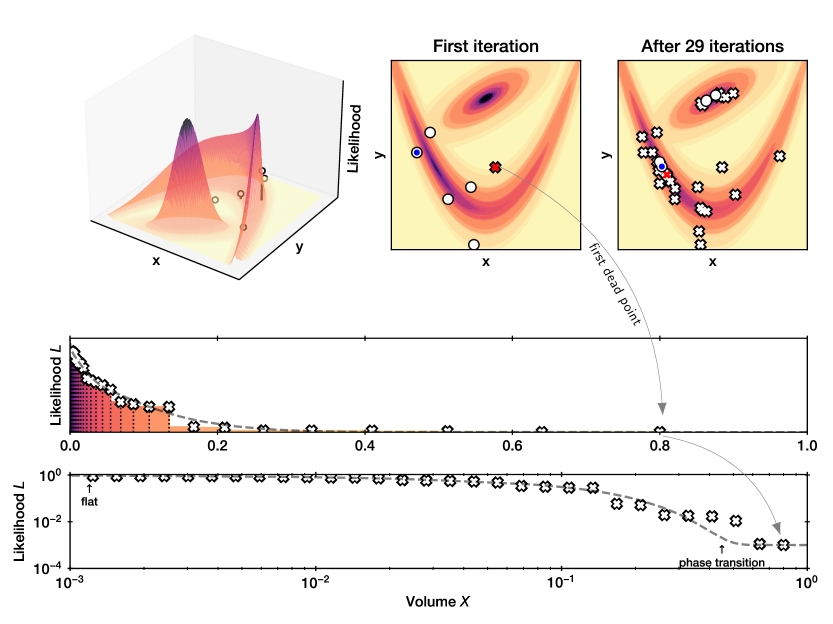
Figure 1: Top left: A complicated likelihood function is defined over a two-dimensional parameter space. NS begins by evaluating $N=5$ random points. Top center: Each live point (circle) defines a likelihood contour. The lowest likelihood point (red cross) becomes a dead point. It is replaced by a new, live point (blue circle), sampled randomly from the prior but above the contour defined by the dead point. Top right: After a few iterations, the live points concentrate in a small volume at the likelihood peak. Bottom panels (top is linear, bottom is logarithmic): For each iteration, a dead point is placed with its likelihood and the prior volume estimated by geometric shrinkage. The prior volume of the sequence shrinks exponentially from right to left. Vertical bars represent the likelihood shell removed, and are coloured consistent with the contours shown in the other panels. The bar area is the posterior weight, and the sum of the bars gives the marginal likelihood $Z$. The gray dashed curve indicates the true volume-likelihood relation for this function. In the bottom log-log plot, the phase transition is marked, which corresponds to the transition from the wide, shallow yellow regions to the high and steep orange regions in the upper panels.

Iterations

We repeat replacing live points (shrinking and LRPS steps), which continuously increases the likelihood threshold and shrinks the volume by approximately a constant factor. Put in another way, removing the lowest point of $N$ automatically chooses likelihood thresholds such that the volume decreases by a constant factor, at least on average. NS scans the prior from the worst to best likelihood. The progression by constant shrinkage factors reduces the remaining volume exponentially.

Termination

After $i$ iterations the remaining volume is exponentially small, $V_{i}=\left(1-\frac{1}{N}\right)^{i}$, with a high likelihood threshold selecting live points close to the best-fit parameter peak(s), i.e., the likelihood of the remaining points is flat. Further $\Delta V_{i}\times L_{i}$ contributions to $Z$ are thus negligible and the integration can be stopped. The algorithm has converged in the sense that iterating further would not significantly alter the result. Other termination criteria are discussed in §4.3.

Integration

Removing a point at iteration $i$ reduced the volume $V_{i}=(1-\frac{1}{N})^{i}$ by $\Delta V_{i}=V_{i}-V_{i-1}=(1-\frac{1}{N})^{i}\times\frac{1}{N}$. This can be envisioned as a shell of prior volume being peeled off. The “level height” for this integration contribution is just the likelihood of the dead point, $L_{i}$. Accordingly, each dead point is assigned the unnormalised weight $\Delta V_{i}\times L_{i}$, and the integral $Z$ is simply: $Z\approx\sum_{i}\Delta V_{i}\times L_{i}$, with an error estimate available. The remaining live points at termination can also be included, with their likelihoods multiplied by the remaining volume distributed equally among them, $V_{i}/N$. The weighted dead points are approximate samples from the posterior, and can for convenience be resampled proportional to $\Delta V_{i}\times L_{i}$ into unweighted posterior samples.

Properties

Figure 1 illustrates some important aspects of this procedure. Firstly, NS defines an initialisation and termination point, and can thus run without the user in the loop. It performs a global exploration of the parameter space. This makes NS robust to identify and characterise multiple modes. The scanning from the entire volume to progressively smaller regions is done by an ever-increasing $L$ threshold. The shrinkage is done by constant factors, which means the $L$ level is increased dynamically. This handles heavy and light tailed distributions equally well. Additionally, it traverses phase transitions, such as from the yellow plateau to the orange base of the modes in Figure 1. This phase transition is highlighted in the bottom panel of Figure 1, where first the likelihood stays approximately constant as the volume shrinks, then increases rapidly, making the $\log X-\log L$ curve non-concave.

The volume-likelihood plot in the second-to-bottom panel of Figure 1 shows that much of the space in this simple example has a very low likelihood, which contributes little to the integral. NS needs to traverse this space, sometimes for a long time, until the bulk of the posterior is reached.

The geometric discovery of new points is done based on the prior. The likelihood function is queried as an oracle for a binary decision, namely, whether a suggested new point is inside or outside. In this geometric sampling of the prior space, NS does not require likelihood function gradients, making it easy to integrate with complex, numerical likelihoods from legacy codes.

Finally, NS terminates unsupervised, when the remaining live points occupy a tiny prior volume, which contributes vanishingly little to the integral.

To summarise, NS is an attractive algorithm framework for Bayesian inference because

1. it explores the parameter space globally,

2. it handles multi-modal distributions and phase transitions well,

3. it initialises and terminates at a well-defined point without cumbersome supervision, and

4. it provides both the marginal likelihood and posterior samples.

3.2 Viewpoint for theoretical statisticians

To solve the $d$-dimensional integral of the joint distribution of $\theta$ and $D$,

$$Z=\int\cdots\int P(D|\theta)\times\pi(\theta)\,d\theta_{1}\cdots d\theta_{d},$$ (1)

NS transforms it into a one-dimensional integral. The survival function of a likelihood-restricted prior is (Chopin and Robert, 2007a, 2010):

$$X(L_{\mathrm{min}}) =pr\{L(D|\theta)>L_{\mathrm{min}}\}$$

$$=\int_{L(D|\theta)>L_{\mathrm{min}}}\pi(\theta)\,d\theta$$

Then a “sorting” of the prior space via the likelihood function is achieved by the inverse:

$$Z=\int_{0}^{1}L_{\mathrm{min}}(X)\,dX$$ (2)

At first glance, this conceptual transformation has not achieved anything, because the relevant multi-dimensional spaces cannot be identified with $L_{\mathrm{min}}$ in all but the most trivial functions.

Instead, NS chooses the $L$ levels such that the corresponding $X$ can be estimated. Note that the inverse of $X$, $L_{\mathrm{min}}(X)$, is a monotonically increasing function. It is visualised in the bottom panel of Figure 1. Suppose $\theta_{1},\ldots,\theta_{N}$ are i.i.d. samples from the prior, and their likelihood is $L_{1},\ldots,L_{N}$. By definition, the survival function of these likelihood samples is $X$. Therefore, the probability integral transform of the samples, $X(L_{1}),\ldots,X(L_{N})$ is i.i.d. standard uniform distributed. The implication is that points sampled from the prior generate $L$ levels uniform in the prior volume $X$. Lets assume the samples were indexed so that $L_{1}=\mathrm{min}\{L_{1},\ldots,L_{N}\}$. Then by the properties of order statistics of a collection of uniform random variables, the corresponding $X_{1}$ follows $X(L_{1})\sim\mathrm{Beta}(N,1)$ (Skilling, 2004). Section 4.2 below discusses alternatives for this step with different assumptions.

Setting $L_{\mathrm{min}}=L_{1}$ and repeating the sampling procedure with the prior restricted to $L(D|\theta)>L_{\mathrm{min}}$ induces nested sampling. The recursion tracks an ever-shrinking $X$ with an ever-increasing likelihood threshold $L_{\mathrm{min}}$. Within the restricted prior space, $X(L_{2}),\ldots,X(L_{N})$ are also uniformly distributed, specifically from $X(L_{\mathrm{min}})$ to unity. The sequence of sampled $X_{i}$ thus has the property $X_{i+1}/X_{i}\sim\mathrm{Beta}(N,1)$, with $X_{1}=1$. This makes estimators such as $Z=\sum_{i}\left(X_{i-1}-X_{i}\right)\times L_{i}$ computable. Section 4 discusses convergence proofs and construction of unbiased integral estimators for $X$, $Z$ and $\log Z$.

Above, only a very brief introduction of the ideas involved in NS was given. We refer to interested reader to Chopin and Robert (2010) and Schittenhelm and Wacker (2020), for more formal introductions, to Walter (2017) for an analysis of the Monte Carlo point process occurring in the sequence of finite ordered points used to track shrinkages by sampling from one likelihood threshold to the next, and Salomone et al. (2018) for connections to Sequential Monte Carlo.

The popularity of Markov Chain Monte Carlo (MCMC) makes it worthwhile to draw comparisons between the two iterative Monte Carlo algorithms. From a starting point, Random Walk Metropolis MCMC constructs a sequence of points. For choosing the next point, a proposal or transition kernel needs to be defined, and the Metropolis acceptance rule either chooses the proposed point or the current point as the next point, proportional to the posterior probability ratio. If chains are run infinitely long, the distribution of chain points converges to the posterior distribution. The performance of MCMC with finite chains crucially depends on the transition kernel, and many methods have been proposed. Similarly, the performance of NS crucially depends on the LRPS, and many methods have been proposed.

The MCMC and NS algorithms can also be qualitatively compared by their emergent behaviour in typical applications. MCMC typically exhibits an initial phase where it attempts to identify the posterior bulk. In this phase, the posterior density is typically rapidly increasing by orders of magnitude. This initial phase is followed by exploration of the posterior, where the chain begins to converge, and the number of effectively independent samples is proportional to the length of the chain.

We can also identify three emerging phases the NS algorithm exhibits. Initially, the volume is large and the live points vary by many orders of magnitude, including many bad fits, so that the dead points receive weights $\Delta V_{i}L_{i}$ that are ultimately negligible. Because the live points vary in their likelihood value by many orders of magnitude, if the algorithm were terminated in these iterations, all of the posterior weight would be concentrated in the most likely point found so far $Z\approx L_{i}V_{i}/N$. Where the volume is still substantial and likelihoods are high, so that $L_{i}\times V_{i}$ is maximal, the posterior bulk is reached, which we can identify as a second phase. Here, multiple points receive comparable weights $V_{i}L_{i}$, i.e., the posterior becomes resolved into multiple posterior samples. Because NS needs to track the shrinkage, it cannot rapidly skip ahead to this phase like MCMC, and therefore (but see §6.2) the phase of identifying the posterior bulk can take many iterations (proportional to the information gain (Skilling, 2004)). Finally, NS exhibits a phase where the likelihoods are high and very close to the maximum likelihood, but the volume has become very small. Therefore, most points receive a small weight and the posterior bulk has been passed. Here NS differs from MCMC in that continuing the run does not linearly increase the effective sample size. Section §3.4 and §6.2 discuss methods for bulking the posterior samples with additional iterations.

3.3 Viewpoint for physicists

Many Monte Carlo algorithms stem from analogies to physical systems. To give an example (from Skilling, 2012; Habeck, 2015), consider several gas particles in a box. The position and velocities of all particles then completely describe the microstate, or configuration $\theta$ of the system. If the particles are rolling under gravity within a (perhaps strangely shaped) basin, the total potential energy of the system $E(\theta)$ can be identified. This is the analogy to the negative log-likelihood, $E(\theta)=-\log L$. NS initially generates random particle configurations. The hottest configuration (highest $E(\theta)$), with energy $\epsilon$ is selected. New configurations $\theta^{\prime}$ accessible with a lower energy state $E(\theta^{\prime})\leq\epsilon$ than the current energy limit are generated, for example by jittering the particles.

Iteratively replacing the hottest configuration by a cooler configuration corresponds to a cooling schedule. Monte Carlo cooling schemes are known from simulated annealing (e.g., Kirkpatrick, Gelatt and Vecchi, 1983) and parallel tempering (Swendsen and Wang, 1986). NS differs here by choosing the cooling schedule adaptively, and that it explores a truncated basin geometrically rather than a smoothed basin proportionally. During the cooling process, it can occur that the energy changes very little, while the volume keeps decreasing, followed by an abrupt change of behaviour where the energy increases rapidly. Such phase transitions (see e.g., Raghavan and Cohen, 1975, for physics background) are problematic in simulated annealing because it considers the magnitude of energy changes. In contrast, because NS progresses with constant speed in volume and considers only the order of the live points, it traverses phase transitions without issue (Skilling, 2004). For plateaus, see §4.5.2.

NS considers an isolated system with a maximum energy (microcanonical view) rather than the ensemble average (canonical view). More explicitly, Habeck (2015) identified several terms from statistical mechanics in the NS procedure, as follows: The volume of configurations $X$, with less energy than a threshold $\epsilon$, is

$$X(\epsilon)=\int_{-\infty}^{\epsilon}g(E)dE,$$

where the density of states at energy $E$ is (see also Cameron and Pettitt, 2014):

$$g(E)=\int\delta(E-E(\theta))\pi(\theta)d\theta$$

In probability terms, $g(E)$ describes the distribution of negative log-likelihood values marginalised over the prior, with $X(\epsilon)$ its cumulative probability distribution. The logarithm of $X$ can then be identified as the microcanonical entropy $S_{G}(E)=\log X(E)$, while the logarithm of $g$ is the surface entropy $S_{B}(E)=\log g(E)$. A microcanonical temperature can then be defined as $T_{G}=X(E)/g(E)$. The total energy of all configurations, the partition function $Z$, is defined as $Z=\int e^{-\beta E(\theta)}\pi(\theta)d\theta$ with $\beta=1$, which is evaluated by NS as $Z=\int e^{-E}g(E)dE$, i.e., over the energy levels. For more details, see Habeck (2015) and Cameron and Pettitt (2014).

The generation of new configurations can also be considered in analogy with physical systems. In this case, each configuration is considered a particle, which inhabits an energy potential. The acceleration of a particle in an energy basin can be motivated as in the development of Hamiltonian Monte Carlo (HMC, Neal et al., 2011). HMC constructs trajectories using the potential energy, which can be considered Keplerian orbits (Betancourt, 2017) of random orientation. NS and HMC analogies differ in two important ways. HMC trajectories conserve the total energy, partitioned into potential and kinetic energy. This tends to explore only a narrow range of potential energies, set by the number of dimensions, and limits HMC’s exploration of new configurations (such as distant basins). In contrast, NS scans potential energies from hottest to coolest, and generates configurations at all energy levels. The second difference is that NS searches for new configurations regardless of their energy, so long as they fulfil the energy threshold. Thus, the particles receive no acceleration, and the exploration is purely geometric. We refer the reader to Nielsen (2013); Martiniani et al. (2014); Habeck (2015); Baldock et al. (2016) for formulations of NS based on statistical mechanics, and for billard-like walks, to §5.1.3.

3.4 Viewpoint for computer scientists

In computer science, to quickly narrow down a search space, divide-and-conquer algorithms such as binary search or k-d trees are frequently employed. Often, algorithms are closely identified with a specific data structure that fully represents the state at any time. It can be insightful to investigate the properties of such data structures. In this section, we identify such a data structure, and phrase NS as an algorithm operating on it. The representation makes resuming an existing NS run, parallelisation and dynamically varying the number of live points trivial, and avoids a special treatment of the final phase of the algorithm.

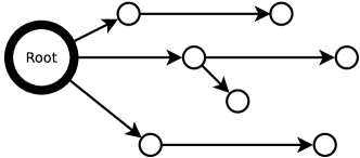
Figure 2: NS exploration presented as a tree. The root node presents the entire volume, with likelihood zero. Each node represents a point sampled from the prior, restricted to be above the likelihood threshold of its parent node. In this presentation, the nodes are also ordered from left to right by likelihood value. Each outgoing edge splits the volume associated with the parent and donates its child a volume of $\frac{1}{N}$ where N is the number of parallel edges.

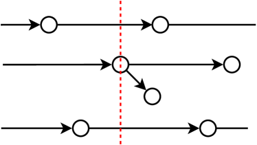
Figure 3: Search operation: The breadth-first search iterates in order of likelihood (from left to right). The number of live points $N$ is the size of the node list, and corresponds to the number of parallel edges (here: three before the red dashed line, four after). The volume is reduced, the node assigned a posterior weight, and the integral updated.

⬇

1function NS-BFS:

2 given root node (representing the prior volume)

3

4 let Q be a list, sorted by likelihood value

5 add all children of root node to Q

6

7 Z = 0

8 V_remaining = 1

9 posterior_points = []

10 posterior_weights = []

11

12 while Q is not empty:

13 Nlive = length of Q

14 obtain and remove next node from Q

15

16 # optional:

17 node_expanding_agent(node, Q, Z, V_remaining)

18

19 removed_fraction = 1 / Nlive

20 remaining_fraction = 1 - removed_fraction

21 V_dead = V_remaining * removed_fraction

22 weight = V_dead * node.likelihood_value

23

24 add node to posterior_points

25 add weight to posterior_weights

26 Z += weight

27 V_remaining *= remaining_fraction

28

29 add all children of node to Q

30 return Z, posterior_points, posterior_weights

Algorithm 1 NS as a breadth-first search algorithm.

We adapt breadth-first search on a tree structure (see Figure 2). The search starts from an initial node and keeps a sorted list of nodes yet to be explored. Initially, the NS tree is a lone root node representing the full prior volume. Next, we consider sampling $N$ random points inside that volume. This is represented by adding $N$ child nodes of the root node, and illustrated in Figure 2. We assign the child nodes their likelihood value. A simple breadth-first search algorithm starts from the root node, keeps a list of “open” nodes, and repeatedly explores the one with the lowest likelihood value until the list is empty. The remaining volume, integrated likelihood and posteriors are also computed. This is presented in Algorithm 1, and illustrated in Figure 3.

The formulation in Algorithm 1 is elegant, because it unifies the nested sampling phase and the remainder integration: During the remainder integration, none of $N$ parallel nodes have children, each removed node shrinks that volume by $(N-1)/N$, leading to equal weights in this phase.

Figure 4: Insertion operation: Adding a child node (right) to the tree means LRPS sampling under the likelihood threshold of that parent node (left).

This procedure would soon run out of nodes to explore, so an agent is needed which adds children to nodes. Figure 4 illustrates that adding a child to a node means LRPS sampling a new point using the parent’s likelihood as the threshold. The simplest formulation with a constant number of live points adds a single child node to each node being passed, and stops when the remaining volume is negligible. This agent is shown in Algorithm 2. In general, an arbitrary number of agents can add children to arbitrary nodes in the tree.

⬇

1function classic_node_expanding_agent:

2 given node # current node

3 given Q # current list

4 given Z # current integral estimate

5 given V_remaining # volume left to be explored

6 Lmax = (last node in Q).likelihood_value

7 frac_remaining = Lmax * V_remaining / Z

8

9 if frac_remaining > 0.001 and node has no children:

10 new_node = LRPS(node.likelihood_value)

11 add new_node as a child of node

Algorithm 2 Exploration agent corresponding to constant-$N$ nested sampling.

This formulation implies that resuming an interrupted run is trivial, if the tree is kept. Also, several NS runs as specified in Algorithm 1 and 2 can run independently in parallel. For merging, all that is needed is to merge the root nodes, and run only the integration of Algorithm 1 for the final result. The formulation also suggests a procedure for converting previously sampled points with their thresholds into a tree: a LRPS sampled point can be attached as a child to nodes with likelihood above or equal the used sampling threshold.

3.5 Components of nested sampling implementations

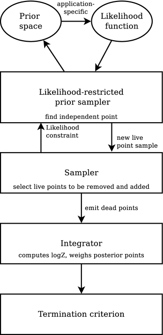
Figure 5: Components of a nested sampling implementation.

To discuss NS in a structured fashion, we identify components of nested sampling implementations. These are illustrated in Figure 5. The core (centre) is a NS sampler which keeps a set of live points, and the likelihood constraint defined by the most recent dead point. At each iteration, the lowest live point may be replaced by a LRPS, which uses the application-specific likelihood function and prior space definition provided by the user. The dead point is passed to the NS integrator, which weighs these dead points to form a posterior sample, and estimates the marginal likelihood $Z$ (see formulas in §3). The following sections discuss the individual components, including the integrator (§4), the termination criterion (§4.3), the LRPS variants (§5) and samplers (§6).

4 Integration

4.1 Theory

NS was introduced in Skilling (2004); Skilling et al. (2006). Convergence and unbiasedness was discussed and proven in Evans (2007); Chopin and Robert (2010); Skilling (2009); Keeton (2011). Making advances to analyse NS theoretically has been the focus of a few publications (e.g., Khanarian and Alvarez, 2013). We refer the interested reader to Walter (2017), which makes connections to the mathematical theory of rare event simulation and the last particle algorithm, and Salomone et al. (2018), which draws connections to Sequential Monte Carlo, nearly considering NS as a special case of that framework. Birge, Chang and Polson (2012) presents a generalisation of NS and connects it to path and bridge sampling, while Polson and Scott (2014) discusses connections to, among others, slice sampling. Chopin and Robert (2007a) and Feroz et al. (2013, appendix C) prove that posterior samples from nested sampling approximate the true posterior for continuous and discontinuous functions, respectively.

4.2 Estimators

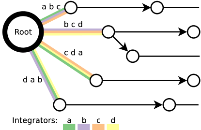
Figure 6: NS error estimation with K-fold cross-validation: Four integrators are invoked, which each are made oblivious to some of the root children (colours). The spread of integration results provides an error estimate.

NS rests on being able to estimate the volume (shrinkage) at each iteration, and that the LRPS samples faithfully. LRPS issues are discussed in §5, while for the discussion here, it is assumed that the LRPS is sampling perfectly. This case is called the idealised algorithm in Guyader, Hengartner and Matzner-Løber (2011), and perfect nested sampling in Higson et al. (2017).

NS rests on being able to estimate the volume (shrinkage) at each iteration. Only in special circumstances the volumes are known precisely (Chopin and Robert, 2008). In general they can only be estimated. Casting the volume shrinkage as a Poisson process yields the volume shrinkage estimator $\delta V=\frac{1}{N}$ (Huber and Schott, 2010; Guyader, Hengartner and Matzner-Løber, 2011). Based on this approach, Walter (2015) derived an unbiased estimator of $Z$. Chopin and Robert (2007a); Evans (2007) and Skilling (2009) discussed whether the ultimate goal is to obtain an unbiased estimator with minimal variance of $\log Z$ or $Z$ (see also Keeton, 2011). Skilling (2009) argued that because Bayes factors and posterior odds ratios interpreted on log-scales are the goal, unbiased estimators of $\log Z$ should be sought.

Integral estimators rely on estimating the compression ratio at each iteration. In the order statistics approach of Skilling (2004), they obtain $V_{i+1}/V_{i}\sim\mathrm{Beta(N,1)}$, and estimate a geometric log-volume progression as $\log V_{i+1}/V_{i}=-1/N$. The mean of the Beta distribution gives $\delta V=\frac{1}{N+1}$, which differs from the unbiased estimator above. Even if not optimal, a slightly biased estimator is suitable for Bayesian inference if its bias is negligible relative to its root-mean-square error. This is the case for the above estimators and their differences, when $N\gg 1$, e.g., $N=100$ (Salomone et al., 2018). For theoretical and online error analyses of the estimators, we refer the reader to the above works.

The termination of the iterative procedure can also induce a bias (Walter, 2015). Walter (2015) explores the use of families of estimators, each corresponding to a different random termination, to remove this bias.

The finite resolution of the $N$ live points leads to a noisy exploration and likelihood fluctuations (Higson et al., 2018). This can be practically and elegantly addressed by sub-sampling (first proposed by Higson et al., 2018). In the tree formulation of §3.4, some of the root children can be unlinked in a bootstrapping or K-fold fashion. This is illustrated in Figure 6. In the tree search formulation one could have several integrators which see only some of the root children, and use the spread of integration results (posterior and $\log Z$) to measure the uncertainty. The shrinkage volume can be randomly generated at each step (using a $\mathrm{Beta}(1,N)$ distribution, Skilling et al., 2006), which then also leads to a distribution of estimators. Incorporating the two sources of variance with sampling yields realistic uncertainty also for single NS runs (Higson et al., 2018).

4.3 Termination criteria

The question arises when to terminate nested sampling. In the tree formulation (§3.4), this means when agents should stop inserting new children nodes into the tree.

Monte Carlo integration techniques have intrinsic limitations in integrating black-box functions. The spike-and-slab problem illustrates this. In Figure 1, we illustrate a small, high peak (spike) and a wider ridge (slab). If the spike is very narrow, it can go unseen by random samples, which will focus on the wider slab. However, if the spike is very high, it will be crucial for the integral. As John Skilling puts it: “It is impossible to find a flag pole in the Atlantic ocean”. NS integration with sparse sampling may pass the likelihood threshold that separates the spike and slab without ever placing live points into the spike. Thus, a spike will likely go undetected if it is smaller than $V_{i}/N$ (Pártay, Bartók and Csányi, 2010). However, if the spike is located on the peak of the slab, then NS will find it, unless it terminates too early.

For less perverse likelihoods, sensible termination can be determined at runtime. Skilling et al. (2006) proposed simultaneously estimating the information gain ($H$, also employed in an error estimate) during the run and estimating the minimum number of iterations needed to pass the bulk of the posterior as $HN$. Similarly, the sample entropy was considered as a termination criterion. Alternatively, Skilling et al. (2006) suggests comparing the dead point integral $Z_{i}=\sum_{i}L_{i}\delta V_{i}$ with the largest possible live point contribution $Z_{\mathrm{live}}=L_{\mathrm{max}}\times V_{i}$, and terminating when the ratio becomes very small, $Z_{\mathrm{live}}/Z_{i}<\epsilon$, with $\epsilon\ll 1$, for example $\epsilon=10^{-3}$. This is also the agent behaviour implemented in Algorithm 2. This can be further refined with $Z_{\mathrm{live}}=\frac{V_{i}}{N}\sum_{j=1}^{N}L_{j}$, trapezoid rule integration, or bootstrapping, but in practice is not more reliable.

A variety of other termination criteria have been considered. For example, Schöniger et al. (2014) proposes terminating when the LRPS becomes extremely inefficient. Low efficiencies caused by complex degeneracies, can indicate that the model could benefit from reparametrisation (see Papaspiliopoulos, Roberts and Sköld, 2007, for a similar situation with MCMC). Baldock et al. (2016) suggests monitoring the temperature (HMC momenta, see below §5.1.3).

The problem of yet unidentified, hidden peaks cannot be addressed in a general and reliable way with information available during the run. Therefore running a few iterations longer than seemingly needed is most effective in practice. This is what the $\epsilon$ remainder fraction criterion effectively does.

Termination can also be addressed with domain knowledge and reparametrisation. Some likelihoods have absolute upper bounds. For example, in a Gaussian likelihood with measurements $d_{i}$ with fixed uncertainties $\sigma_{i}$ fitted with an arbitrary model $m$, the weighted sum of squared deviations, $\chi^{2}$, is positive: $-2\times\log L=\chi^{2}=\sum_{i}\left(\frac{m(i,\theta)-d_{i}}{\sigma_{i}}\right)^{2}>0$. The likelihood bound directly gives upper bounds on $Z_{\mathrm{live}}$ of future iterations.

4.4 Complexity scaling

We can now consider the computational complexity of NS integration. This depends on (1) the information gain of the posterior compared with the prior (I), which determines the shrinkage necessary to reach the bulk of the posterior, (2) the number of live points, which determines the shrinking per iteration, and (3) the computational complexity of the LRPS per NS iteration to find a reliable new point, which is subject to peculiar degeneracies (P), multi-modality (M) and dimensionality (D) issues.

The NS complexity scales linearly with the number of live points $O(N)$, due to the slower shrinkage (Skilling, 2004). Beyond this, the scaling of the LRPS method can be arbitrarily hampered by complex posterior shapes that need to be navigated until a new independent sample is obtained. Assuming the latter scales linearly with dimensionality $d$, Skilling (2009) gives the cost scaling of NS as $O(d^{2})$. In practice, Handley, Hobson and Lasenby (2015a) demonstrate a scaling of $O(d^{3})$ for their implementation. This makes NS perhaps less attractive for very high-dimensional problems with many thousands of parameters such as fitting large hierarchical Bayesian models or neural networks. However, Javid et al. (2020) demonstrate that neural networks can be fitted, and NS is attractive because the global exploration avoids choosing overly complex networks.

However, the relation between cost and live points is more complex. While convergence slows with the number of live points, some LRPS methods work more efficiently the more live points, as they help map out the likelihood constraint and can identify the approximate neighbourhood where new points are likely successful (see §5). Following Allison and Dunkley (2014), this is illustrated with the ellipsoidal rejection sampling technique (discussed further in §5.2) for the case of ellipsoidal, mono-modal likelihoods. For this, the LRPS cost per iteration is empirically found In Appendix B to scales as:

$$O(C_{\mathrm{ell}})=\exp\left\{\left(\frac{6.83\times d^{1.9}}{N}\right)^{3/4}\right\}$$ (3)

The exponential increase becomes crucially important when the number of live points is small. This likely encodes the curse of dimensionality, and the inherent limitations of rejection techniques. Equation 3 suggests that the number of live points for ellipsoidal sampling should not be lower than $7\times d^{2}$.

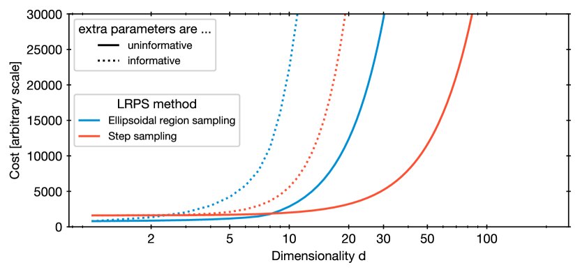
Figure 7: Number of likelihood evaluations on Gaussian-like likelihood functions. The blue curves show two cases with different information gain changes with dimensionality. Both cases indicate a low cost at $d<30$ dimensions for ellipsoidal NS under optimal conditions (likelihood with ellipsoidal contours). Red curves illustrate the shallower, polynomial scaling of step samplers.

The total cost is obtained from the per-iteration cost and the number of iterations needed. Shrinking from the prior volume $V_{p}$ until a low fraction $\epsilon$ of a target posterior volume $V_{t}$ requires $i=N\times\ln\frac{V_{p}}{V_{t}\times\epsilon}$ iterations (see §3.1). The ratio $H=\ln\frac{V_{p}}{V_{t}}$ here is the information gain from the prior to the posterior. Combining the acceptance rate formula of eq. 3 and the number of iterations $i$, and the sampling of the initial $N$ live points, Allison and Dunkley, 2014 obtain the total nested sampling cost as:

$$C=N+i\times C_{\mathrm{ell}}=N+N\times\ln\frac{V_{p}}{V_{t}\times\epsilon}\times C_{\mathrm{ell}}$$ (4)

The factor $V_{p}/V_{t}$ is problem-specific. It is not easy to study the scaling with dimensionality, as varying the dimensionality implies analysing a different problem. Here we consider two cases: (A) If new parameters are added, and they are all updated with the same information gain, then $V_{p}/V_{t}=K^{d}$. This increases the cost of $C$ to $O(N\times C_{\mathrm{ell}}\times d)$. (B) If adding new parameters only redistributes the same information, then $V_{p}/V_{t}=K$ remains constant with dimensionality, and thus the cost is of order $O(N\times C_{\mathrm{ell}})$. For these two cases, the total costs $C$ are plotted in Figure 7, with $N=400$. The normalisations are arbitrary and cannot be compared. Ellipsoidal NS clearly works best in $d<30$ dimensions. This agrees with our practical experience with the MultiNest ellipsoidal sampling implementation, which begins to break down close to that dimensionality. For comparison, the aforementioned $d^{2}$ scaling of a MCMC LRPS algorithm is also shown as red lines, with an arbitrarily chosen base cost added. Interestingly, the above analysis suggests that for ellipsoidal problems, a $d^{2}$ scaling is possible with ellipsoidal sampling if the live points are increased quadratically. However, the optimistic case where the likelihood indeed has elliptical contours was analysed, while for other cases, the cost may be higher.

In practice, the computational cost is specific to the model structure as well. Thus numerical testing is required (see for example Figure 15 in Pitkin et al. (2017) and Figure 6 in Trassinelli and Ciccodicola, 2020). Finally, the discovery of likelihood peaks is also regulated by $N$ (see §4.4). Because of this, running NS with very small $N$ does not necessarily give useful “quick look” results.

4.5 Correctness diagnostics

How can a complete NS implementation (including integrator, LRPS, sampler, termination criterion) be evaluated for correctness? We can divide in two categories of tests, following Stokes, Tuyl and Hudson (2016).

4.5.1 Outside-in: Application to known functions

Firstly, the NS implementation can be applied to test problems with known properties. The simplest case is likelihood functions where the integral $Z$ is analytically known (e.g., Preuss and von Toussaint, 2007). The main limitation here is that analytic likelihood functions often do not resemble real-world problems. A further problem is that often, for example, when choosing a Gaussian likelihood expression, the integral is dominated by a narrow range of likelihood values. Thus, the LRPS and integration are therefore potentially only tested on a low number of iterations. This can be improved by choosing heavy-tailed distributions. An extreme case is $L=\min(\theta^{-1},e^{100})$ with $\theta$ defined over the unit interval, which makes all dead points yield approximately equal weights.

Secondly, the LRPS can be tested in isolation. Buchner (2014) proposed a LRPS test that verifies that the shrinkage caused by the LRPS behaves as expected ($1-1/N$). This is based on likelihood functions where one can analytically compute the volume enclosed at a given likelihood $X(L)$. For example, in a Gaussian likelihood, the circular likelihood contours can be identified with an ellipsoid. Then, from a sequence of likelihoods obtained from repeated LRPS, volume shrinkages can be computed and compared to expectations. If the likelihood of the found point is systematically lower or higher, then the LRPS is noticeably incorrect. This can be applied to many posterior shapes, including multi-modal Gaussians. A particularly sensitive test is the hyper-rectangle $L=\max_{i}||\theta_{i}-\frac{1}{2}||^{-1}$, because its shape is far from Gaussian and exhibits many corners in high dimensions. Importantly, this test is independent of the tail weight, as the likelihood only enters in NS weighting of points. It can also be applied in very high dimensions to tune LRPS parameters.

4.5.2 Inside-out: Diagnostics at or after run-time

The second group of tests tries to notice during the NS run when assumptions are broken.

Likelihood functions with plateaus can cause problems in nested sampling (Skilling et al., 2006; Schittenhelm and Wacker, 2020). This is because the ordering of the prior space is not available, and a large volume is associated with a vanishing likelihood interval in eq. 2. Therefore, if two live points have the exact same likelihood, this should cause alarm. To address this, Fowlie, Handley and Su (2021) proposed a small modification to the nested sampling algorithm iterations to remove all live points with $L_{\mathrm{min}}$ without replacement before replenishing the live point set to size $N$.

One assumption is that the LRPS samples correctly according to the constrained prior. Stokes, Tuyl and Hudson (2016) proposed tests for uniformity in 2-dimensional problems. Firstly, they count the empty cells in a segmentation, and compare them with a Bayes factor to uniform expectation. Secondly, they develop an equi-distribution test that measures the concentration of samples with an entropy, and compares that to a uniform expectation. Finally, they visualise deviations from uniformity with quantile-quantile plots. These tests however appear limited to very low-dimensional problems.

Higson et al. (2018, 2019) contributed visualisations of the uncertainty in the inference, in particular of the posterior distributions. This is achieved by sub-sampling (see §4.2) completed nested sampling runs, and plotting the spread of posteriors. Relatedly, they propose diagrams of volume ($\log X$) vs. parameter value ($\theta_{i}$), which allows insight into the structure of the parameter space, and how the LRPS replaces samples.

Higson et al. (2019) further proposes testing the variance between multiple independent NS runs to the variance expected from sub-sampling a single run. Here, one can check the expectation for each parameter $\theta_{i}$, a combination $f(\theta)$, or $\log Z$. Excess variance can occur when the LRPS is sampling imperfectly, and its samples and shrinkages are correlated. Higson et al. (2019) also considered the expectations between only two runs, when the computation is very costly.

Finally, Fowlie, Handley and Su (2020) pointed out that if the samples returned from the LRPS are independent and perfectly distributed according to the constrained prior, then where they are inserted into the sorted live points list should be uniformly distributed. They proposed an insertion order test to check this condition. The insertion order of each new sample is collected. The order distribution is tested with a Kolmogorov-Smirnov (KS) test every $N$ iterations, and for the full run. Fowlie, Handley and Su (2020) demonstrates that this works well to detect problematic runs in practice on toy problems. Alternatively, the insertion order test could also be used as a quality indicator. When the test triggers, the sample collection is reset. Then the number of iterations until the test triggers can be interpreted similar to an auto-correlation length in random walk MCMC algorithms. However, the samples collection likely still needs to be truncated occasionally, so that a recent addition of poor samples is not diluted by a preceding high number of good samples. A limitation here is that the KS test as typically implemented is only valid for continuous variables. Fowlie, Handley and Su (2020) show that the rounding to integers makes the distribution non-uniform, and the test is less sensitive than it could be.

We propose an improvement of the power of the test with a statistic suitable for testing whether discrete numbers are uniformly distributed. We begin with the Wilcoxon-Mann-Whitney U test Mann and Whitney (1947), which tests two sequences of observations, of length $n_{1}$ and $n_{2}$. For each observation in the first sequence, the number of smaller and equal observations in the second sequence is recorded (“wins”, $W$), as well as the number of equal observations (“ties”, $T$). Then the $U$ statistic is:

$$U=W+\frac{1}{2}T$$

Then $U$ is normal distributed with mean

$$m_{U}=\frac{n_{1}\times n_{2}}{2}$$

and standard deviation

$${\displaystyle\sigma=\sqrt{\frac{n_{1}n_{2}}{12}\left(n+1-\sum_{i=1}^{k}\frac{t_{i}^{3}-t_{i}}{n(n-1)}\right)}}$$

with $t_{i}$ the number of observations that share order $i$ and $n=n_{1}+n_{2}$. In other words, $z=\frac{U-m_{U}}{\sigma_{U}}$ is approximately standard normal and should rarely exhibit, for example, $|z|>3$, a $3\sigma$ excursion.

$N$	Coverage	KS test	U test
1000	0.9	1.00000	0.99723
1000	0.96	0.13472	0.19984
1000	0.98	0.01416	0.02627
400	0.9	1.00000	0.69506
400	0.96	0.02344	0.04745
400	0.98	0.00589	0.00926
100	0.9	0.07364	0.07745
100	0.96	0.00988	0.00771
100	0.98	0.00593	0.00383

$N$	Slant	KS test	U test
1000	0.9	0.31010	0.44932
1000	0.96	0.01864	0.02873
1000	0.98	0.00505	0.00728
400	0.9	0.06385	0.11478
400	0.96	0.00635	0.01084
400	0.98	0.00343	0.00425
100	0.9	0.01205	0.01653
100	0.96	0.00419	0.00363
100	0.98	0.00335	0.00281

Table 1: Performance comparison of KS test and U test. In the left table, the integers are distributed from $0$ to $N\times\mathrm{Coverage}$, in the right table they are distributed with probability $p_{i}\propto i^{\mathrm{Slant}}$. The fraction of tests reporting a $3\sigma$ significance ($p<0.0027$) is reported on the right. The U test fractions are higher in almost all cases.

Lets now imagine that the second sequence is a very large sample of reference points ($n_{2}=N\times M$ with $M\gg 1$). They are uniformly spread from $0$ to $N-1$, thus each order is represented by $M$ samples. The first sequence of observations are the collected insertion orders, $O_{i}$. These are integers ranging from $0$ to $N-1$. In that case, a observed insertion order $O$ will have $M$ ties and $O\times M$ wins. The test statistic becomes:

$$U=M\times\sum_{i=1}^{n_{1}}\left(O_{i}+\frac{1}{2}\right)$$

The mean becomes $m_{U}=\frac{1}{2}\times n_{1}\times N\times M$ while the standard deviation simplifies because $M\gg 1$ and $n_{2}\gg n_{1}$, to ${\displaystyle\sigma=\sqrt{\frac{n_{1}}{12}}\times N\times M}$. Cancelling out $M$ which occurs in $U$, $m_{U}$ and $\sigma$, we find that

$$z=\frac{\left(\sum_{i=1}^{n_{1}}\frac{2O_{i}+1}{N}\right)-n_{1}}{\sqrt{n_{1}/3}}$$

is standard normal distributed. This is easy to numerically confirm by sampling $n_{1}$ integers sampled uniformly in $[0,N)$ and plotting the $z$ values. We make two important remarks: Firstly, in this form, the $U$ test allows $N$ to vary from iteration to iteration. Secondly, the sign of the $z$ statistic indicates the direction of the bias.

Now the sensitivity of the KS test and the $U$ test (both two-sided) can be compared. For reasonable numbers of live points, two scenarios are considered in Table 1: In the first simulation (top), generated insertion orders are truncated to only cover the range $0$ to $\left\lceil N\times C\right\rceil$, with $C<1$. In the second simulation (bottom), generated insertion orders are simulated from a mildly slanted power law distribution, with order $i$ more likely at the low end. We simulated $100,000$ samples of size $N=1000,\,400,\,100$ and apply the KS and $U$ tests. The fraction of tests reporting a $3\sigma$ deviation are compared in Table 1. In general, the U test has a higher detection rate. However, when the detection rate is already high ($>50\%$), or very close to the expected false positive rate, the KS test sometimes performs similarly or better. However, these are less interesting edge cases. Additional to being more sensitive, the U test is slightly simpler to implement, as only $\frac{2O+1}{N}$ and the number of samples $n_{1}$ need to be accumulated, instead of entire histograms.

The test can be applied in three different ways: (1) on the full run as in Fowlie, Handley and Su (2020), (2) every $N$ iterations (Fowlie, Handley and Su, 2020), probably with a Bonferroni correction, and (3) accumulate until $|z|$ exceeds a predefined threshold. For example, when simulating $10^{7}$ iterations with uniform insertion order, resetting the accumulation statistic when $|z|>4$ leads to segment lengths no shorter than $10^{5.5}$. If shorter segments are regularly produced, or more specifically, if the number of segments of a NS run is larger than the number of iterations divided by $10^{5.5}$, this is an indication that the run is biased. This option avoids selecting a chunk size to apply the test.

5 Likelihood-restricted prior sampling (LRPS)

LRPS is the crux of NS. Empirical statements about what NS can or cannot do are at the mercy of the LRPS implementation. This section tries to convey that a large diversity of solutions are possible and have been considered.

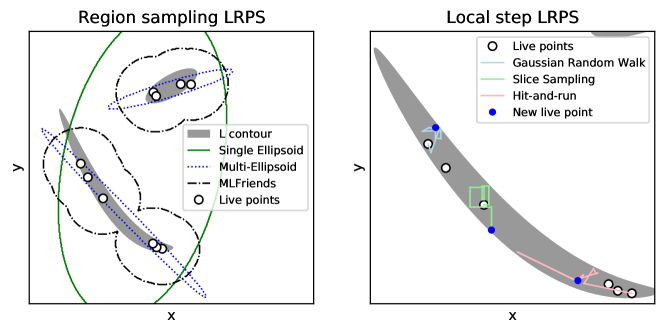
Figure 8: LRPS methods. At an iteration for the example from Figure 1, different methods for finding a new live point are illustrated. Left panel: Region sampling methods construct regions based on the live points (white circles) to approximate the unknown likelihood contour (grey). Rejection sampling based on these contours becomes inefficient if the contours are too large, and problematic for NS integration if it misses a region (e.g., the top left tail). The enlargement is intentionally chosen too small here. Right panel: Local step methods start Metropolis random walks (coloured lines) from a live point (white circle). Steps outside the likelihood contour are rejected. If the step proposal is good and the number of steps large, a new point (blue circle) is reached that is independent of the starting point.

LRPS is supposed to deliver an independent, new point sampled from the likelihood-restricted prior. This can be difficult to achieve perfectly. However, in practice, and as elaborated in Salomone et al. (2018) with theoretical arguments, good NS results can be achieved also with mildly correlated points.

5.1 Local step algorithms (MCMC-based)

A new point can be sampled from the prior with MCMC (Skilling, 2004). Typically, either the recently deceased point, or a random point are chosen as the start of a random walk, or more generally, invariant move steps with respect to the constrained prior. A new point is proposed, and accepted if it exceeds the current likelihood threshold. In flat priors, this makes the random walk a purely geometric exploration. Such random walks are illustrated in the right panel of Figure 8. The random walk proceeds for a number of steps, after which the final point is returned to the NS sampler as a (nearly) independent sample.

Any random walk MCMC solution to LRPS needs (1) a step proposal, (2) a recipe for adapting the proposal to the continuous shrinking as NS progresses and (3) the number of steps. Unfortunately, the literature often lacks these implementation details which severely limits the usefulness of numerical comparisons.

5.1.1 Leveraging live point knowledge

To craft a good step proposal, two properties can be leveraged: Firstly, the current live points are already distributed at least approximately according to the current contour, and trace out the relevant space and its geometry, if they have been sampled faithfully from the prior up to the current iteration. This assumption is certainly justified for the initial live points, which are drawn directly from the prior. Secondly, the behaviour of the contour changes little from iteration to iteration, as the volume shrinks by a small fraction, so that very similar problems have to be solved in sequence.

The second property is leveraged by reusing optimised proposals between iterations, for example if the previous iteration’s acceptance rate was low, the proposal is shrunk before use in the next iteration (e.g., Sivia and Skilling, 2006). However, such adaptions do not maintain detailed balance. To address this, Salomone et al. (2018) suggest a warm-up NS run with adaptive proposals turned on and stored for each iteration, and followed by a final run that uses these proposals, now without adaptations.

The first property is leveraged by many authors by estimating the sample covariance from the live points (Veitch and Vecchio, 2010; Schuet, Timucin and Wheeler, 2011) or determining the principal directions (Nikolic, 2009) to understand size and orientation of the current space.

More sophisticated procedures are necessary to handle multi-modality. Martiniani et al. (2014) pre-computes a database of minima and performs an exchange move, whereby the MCMC can swap between them. Taking advantage of the live points, Handley, Hobson and Lasenby (2015b) performs iterative Jarvis-Patrick clustering (Jarvis and Patrick, 1973) and then estimates covariances based on the member points of each cluster, obtaining a local covariance used for walks started from members of that cluster. MCMC schemes originally intended for unimodal distributions can be extended to handle multiple modes by applying a clustering algorithm to the live points, overlaying the cluster points by subtracting cluster means from member points, and to derive the proposal from the shifted points (e.g., their sample covariance). Then the MCMC algorithm begins its chain from a random live point as its starting point.

5.1.2 Sampling by vicinity

The first fully specified proposal was presented in Sivia and Skilling (2006). A multi-dimensional Gaussian is used, starting from the dead point. If the number of accepts $a$ dominates the number of rejects $r$, the standard deviation is increased by a factor of $\exp(1/a)$, otherwise decreased by a factor of $\exp(1/r)$. Brewer, Pártay and Csányi (2011) prefers a heavy-tailed, highly multi-scale proposal to avoid adaptation at the current iteration. Numerous other MCMC proposal distributions have been applied (e.g., Liu et al., 2016; Beaton and Xiang, 2017; Polido, Jablonski and Lépine, 2013). A Gaussian random walk is illustrated with blue lines in the right panel of Figure 8.

Another solution comes from Veitch and Vecchio (2010), who uses a Student-t distribution with 2 degrees of freedom proposal scaled to 10% of the covariance of live points, estimated every 10 iterations. However, 10% of steps use a proposal inspired by differential evolution: two additional live points are selected, and the difference vector added to the current point. These attempt to address multi-modal distributions; however, they observe that for a specific problem even with 1000 MCMC chain steps, LRPS artefacts remain. For higher efficiency in intermediate or high dimensional problems, Gibbs (Murray et al., 2006) and component-wise proposals along the principal components Nikolic (2009) have been proposed. Trassinelli (2016) primarily uses per-parameter MCMC proposals with a uniform distribution, but also includes a crossover step to combine live points. This work does not verify the correctness of their implementation. A later publication by the same author includes MCMC proposals that do not preserve detailed balance (Trassinelli, 2019, their first high-failure recovery procedure).

To incorporate knowledge of the problem parameter space geometry, Javid (2019) introduced proposals along spherical arcs and wrapping of circular parameters.

Moss (2020) deforms the proposal space to flatten peculiar shapes and bring multi-modal distributions together. A neural network is optimised to transform the live points with least information loss to a standard Gaussian distribution. Sampling from that simpler surface can be more efficient, and if proposals consider the space compression by the non-linear flow via the Jacobian, samples from the (restricted) prior can be obtained. This method appears to be very promising and general, but also complex to implement and train correctly in practice.

5.1.3 Sampling by direction

Betancourt (2011) derived Constrained Hamiltonian Monte Carlo (CHMC), the straightforward application of Hamiltonian Monte Carlo to likelihood constrained prior sampling. For simplicity, we describe its behaviour in a suitable parametrisation where the prior is flat. Then CHMC makes straight steps of length $\xi$ in a chosen direction until the step violates the constraint. There, it reflects off the boundary, i.e. the momentum vector reverses normal to likelihood (constraint) gradient, and continues. This technique thus requires a step size and a computable likelihood gradient. Galilean Monte Carlo (GMC; Skilling, 2012) adds a reverse step to CHMC upon rejection of the reflection, so that the chain succeeds more often. This technique is related to reflections discussed in Neal (2003). Demonic Nested Sampling (Habeck, 2015) softens the likelihood contours by storing excess likelihood (energy) in a demon. This means that a MCMC procedure then tends to turn away from the border without requiring the use of gradients. When gradients are available, Demonic Nested Sampling can store the CHMC velocity vector, and solve a combined momentum-position space. Baldock et al. (2017) also presents a HMC-based nested sampling extension, and compares GMC with a CHMC version that stores the momentum of each live point, finding them to outperform simpler random walk MCMC algorithms (see also Nielsen, 2013).

Another procedure is the sampling from an existing point along a line. Here, three families of such algorithms are presented, all of which are available in UltraNest:

1) In slice sampling (Neal, 2003), parameter space axes are iterated through for the proposal direction. Uniform sampling is achieved by choosing distant bounds, sampling uniformly between them and shrinking the bound towards that side for every reject until a sample is accepted (Handley, Hobson and Lasenby, 2015b). The slice sampling random walk is illustrated with green lines in the right panel of Figure 8. For non-uniform priors, an additional step is needed, by sampling the height of the prior distribution with an auxiliary variable. For flat priors, or placing slices through a reparameterised space which make the prior flat, the likelihood function is used as an oracle (above the likelihood threshold, or not). The NS literature often remains vague which exact variant of slice sampling is implemented. A positive example is PolyChord, which proposes along principle axis after the next (Handley, Hobson and Lasenby, 2015b). The principle axis are obtained from the sample covariance matrix of live point cluster where the walk has started (see §5.1.1).

2) In hit-and-run Monte Carlo (HARM, Turchin, 1971; Smith, 1984), a random direction is instead chosen in each step. The algorithm variant with bound shrinkage was presented explicitly by Kiatsupaibul, Smith and Zabinsky (2011) and is most closely related to slice sampling. Such a walk is illustrated with pink lines in the right panel of Figure 8. Even in complicated geometries, HARM is highly effective in mixing and scales well with dimensionality (see Collins et al., 2013; Kiatsupaibul, Smith and Zabinsky, 2011, and references therein), Collins et al. (2013) also show that it outperforms slice sampling. Stokes, Tuyl and Hudson (2017) tested this technique for NS with non-convex surfaces, albeit in low dimensions.

3) Drawing the direction by choosing another random live point. For example, Stokes, Tuyl and Hudson (2017) uses a simplex-inspired walk to take advantage of the distributions of live points. Pitkin et al. (2017) combines of several proposals including uniform local step proposals, differential evolution, and affine-invariant ensemble sampling MCMC (Goodman and Weare, 2010). The affine-invariant ensemble sampler is a popular choice for a MCMC proposal, because it does not need tuning. This appears as a natural choice for NS, which already maintains a population of points. However, in practice, this proposal performs well primarily in Gaussian shapes, and Huijser, Goodman and Brewer (2015) demonstrate that in high dimensions, the sampler population collapses into a lower-dimensional plane.

Many more geometric random walk algorithms exist and appear a-priori suitable for LRPS in NS. For example, see the survey by Vempala (2005).

5.1.4 Number of steps for independence

All aforementioned methods require the number of steps until a new, supposedly independent point is found. How to chose the number of steps? This is surely dependent on at least P/D issues. A simple technique is to observe the change of $Z$ in a series of NS runs with increasing number of steps (e.g., Higson et al., 2019).

Alternatively, that the live points are already uniformly distributed suggests a simple tuning criterion. If the local MCMC chain has not progressed further than the typical distance between two live points, it has likely not stepped far enough (Salomone et al., 2018). A simple auto-tuning method is thus to increase/decrease the number of steps for the next iteration when that criterion is reached/not reached. For the typical live point distance, UltraNest’s implementation of HARM auto-tune method (“adapt=move-distance”) uses a mean Mahalanobis distance of all pairs of live points. Salomone et al. (2018) emphasises that for conserving detailed balance, a fresh run with no adaptation has to be performed with a predefined number of steps, i.e., at least as many as auto-tuning determined.

In CHMC and Galilean Monte Carlo, the reflections can lead to cycles that do not explore more of the parameter space with increasing number of steps. To address a similar problem in HMC, Hoffman and Gelman (2014) proposed to construct forward and backward HMC trajectories only until they turn back (No U-turn sampler, NUTS). Detailed balance is preserved by randomly considering going forward or backwards while iteratively doubling the number of steps. A U-turn can be identified when the end point vectors show a positive dot product. A point is then sampled from the trajectory, with acceptance probabilities determined by the total energy (target probability and step momentum). Variants of NUTS may be an interesting research direction for Demonic Nested Sampling extensions.

To transfer this approach to NS, Griffiths and Wales (2019) developed the No Galilean U-Turn Sampler (NoGUTS). In the case of CHMC and Galilean Monte Carlo under a flat prior, the momentum remains constant and the target probability is either a constant or zero. Therefore, the trajectories are straight until boundary reflections. This simplifies the problem compared with NUTS. However, the constant shrinkage of the sampling space in NS leads to biases if simple step size adaptations are employed (Griffiths and Wales, 2019).

To allow good resolution of the sampling space and not stepping out of the boundary too often, Skilling (2012) recommends tuning the step size so that most steps are accepted. This however means that most of the steps constitute the progression of a straight line and contain little additional information. A comparative study of the mixing quality of NoGUTS, HARM and slice sampling in different problems remains unstudied as of yet.

5.2 Region sampling algorithms (non-MCMC)

The safest way to sample from the prior under a likelihood constraint is to sample randomly from the prior and reject the point if the likelihood constraint is not fulfilled. This rejection sampling requires a good proposal function to be efficient. In the case of LRPS, the support of the proposal function corresponds to a parameter space region. For correctness, it must fully contain the (unknown) likelihood contour, i.e., the support of the likelihood-restricted prior. If a portion of the parameter space is left out, as illustrated in Figure 8, the volume ratio $V_{i+1}/V_{i}$ will be overestimated. However, the $Z$ estimate can be over or underestimated, depending on the likelihood in the left-out region relative to the constructed region. The methods presented in this section try to reconstruct this likelihood contour itself, or at least a super-set of it.

Mukherjee, Parkinson and Liddle (2006) compute the smallest bounding ellipsoid that contains all live points, and expands this by a factor ($\sim 1.7$). The left panel of Figure 8 illustrates such an ellipsoid wrapping the live points. Iteratively samples are drawn from the ellipsoid and their likelihood is evaluated (rejection sampling). This method thus has two parameters: The number of live points, which helps trace out the parameter space, and the enlargement factor. If the ellipsoid is not expanded enough, regions of the parameter space are never sampled, if it is expanded too much, the rejection sampling is inefficient. The choice of the enlargement is model and dimension-dependent. Beyond approximating the minimum-volume bounding ellipsoid with a scaled covariance metric, more advanced constrained optimisation algorithms yield smaller volumes (Rollins, 2015). Why would ellipsoids be preferred over, say, a box (used in Obrezanova et al., 2007; Möller et al., 2013)? In the high-data regime, likelihood functions tend to become elliptical distributions (such as a multi-variate Gaussian), which have ellipsoidal contours (see e.g., Wilks, 1938).

If the problem presents multi-modality, the space between modes makes the rejection sampling very inefficient. Therefore, Shaw, Bridges and Hobson (2007) cluster the live points with recursive k-means and employs ellipsoid sampling for each cluster. In contrast, Theisen and Jülich (2013) increases the number of clusters when the sampling efficiency drops below a threshold. Feroz and Hobson (2008) further consider x-means, g-means and pg-means for the clustering and uses x-means in the end. The algorithm chooses the end points of the major axis of the ellipsoid enclosing the live points, and attempts a k-means clustering with two clusters. Live points are assigned to one of the two clusters, and used to construct enclosing ellipsoids. If the two ellipsoids describe the live points better than a single ellipsoid around all live points, the clustering is accepted. This procedure is recursively repeated, until convergence. The condition when a split is accepted needs to be defined, and a variety of criteria are tested in Shaw, Bridges and Hobson (2007); Feroz and Hobson (2008); Feroz, Hobson and Bridges (2009), including information criteria. The perhaps simplest is to consider whether the volume is decreased by at least a certain factor, and whether the ellipsoids are sufficiently apart. The MultiNest algorithm has these criteria as parameters additional to the ellipsoid enlargement factor. The left panel of Figure 8 illustrates the multiple-ellipsoids clustering.

Feroz and Hobson (2008) also considers adaptive enlargement factors that decrease with iteration and ellipsoid volume, but these are ultimately not used in the MultiNest algorithm presented in Feroz, Hobson and Bridges (2009). The use of multiple ellipses is also useful for approximating peculiar shapes. The efficiency has made MultiNest a popular algorithm, with multiple implementations and interfaces, including PyMultiNest (Buchner et al., 2014) for Python, RMultiNest (Buchner, 2015) for R, an unnamed Mathematica implementation (Gervino, Mana and Palmisano, 2016), DIAMONDS for C++ (Corsaro and De Ridder, 2014), JAXNS for the jax GPU programming language (Albert, 2020), nestle (Barbary, 2016) and, derived from the latter, dynesty Speagle (2020), also for Python.

To avoid choosing an enlargement factor for every problem, Buchner (2014) estimates it from the live points by cross-validation. If some random subset of live points were unknown, would we construct a region large enough sample them? If not, the enlargement is insufficient and must be increased. After several cross-validation rounds, a large-enough enlargement is found. As a specific example, the RadFriends algorithm Buchner (2014) turns every live point into the centre of an ellipsoid, whose shape determined by the choice of distance metric. While the original RadFriends used spheres, Buchner (2019)’s MLFriends uses the covariance of live points to define the ellipsoids, leading to substantial speed improvements. The left panel of Figure 8 illustrates the region constructed by MLFriends. Clusters are naturally defined by checking which live points are contained in other live points’ ellipsoids. Subtracting the cluster means from each live point, and taking the resulting covariance improves the geometry further, without requiring a dedicated clustering algorithm.

5.3 Hybrid methods

Hybrid methods combine the region reconstruction with MCMC sampling. These reduce the number of likelihood evaluations by excluding space that is very likely outside the contour, while retaining the dimensionality scaling of MCMC algorithms.

Feroz and Hobson (2008) combined MultiNest with the MCMC proposal of Sivia and Skilling (2006) of 20 steps and tested problems in up to 100 dimensions. Interestingly, they find that using a proposal tuned with local covariances is inferior. Such hybrid combinations are available in dynesty (Speagle, 2020).

Different to MultiNest’s x-means, Trassinelli (2019) explores Gaussian mixture method and the mean-shift clustering method with MCMC, but lacks numerical comparisons to judge any improvements over previous publications, both for the proposal and clustering method.

The UltraNest package can combine two region construction methods, MLFriends and a single ellipsoid. The former works well in low dimensions and with multiple clusters, while the latter works well for Gaussian-like likelihoods. The enlargement factors are estimated in both cases with bootstrapping. New points are only considered when they fall within both region constructions. Step sampling methods can then take advantage of both regions to pre-filter proposed points to avoid model evaluations.

6 Nested sampling variations

In standard NS, the sampler maintains a fixed number of live points. This involves identifying the lowest likelihood point and replacing it with LRPS, thereby increasing the likelihood threshold monotonically. The following subsections look at variations of this scheme, including soft likelihood constraints (§6.1), varying the number of live points (§6.2) and possibilities for parallelisation (§6.3) of the algorithm.

6.1 Softening the hard likelihood constraint

LRPS methods deal with a hard likelihood threshold, and thus can only test whether a point is acceptable or not. Points which turn out to be below the contour are discarded, and it is difficult to know when a random walk trajectory approaches the contour. At the same time, when LRPS methods mistakenly exclude parameter space the shrinking is accelerated, while slow LRPS sampling (such as too short random walks) can cause points not to move enough, leading to slowed shrinkage. To address these problems, methods have been developed which relax the problem by avoiding a hard contour.

Importance sampling draws from an analytic shape to approximate the unknown probability distribution of interest and reweighs the samples. Importance Nested Sampling (INS, Chopin and Robert, 2007b; Chopin and Robert, 2008, 2010) applies the same concept by generalising nested sampling in this fashion. Feroz et al. (2013) employed this concept with multi-ellipsoidal sampling, and demonstrates that the use of otherwise discarded samples leads to a substantially more precise $\log Z$ estimate. Indeed, the INS estimator can somewhat correct for the incorrect LRPS sampling of MultiNest in some difficult problems (Buchner, 2014; Feroz et al., 2013). However, Nelson et al. (2020) demonstrate in an application to exoplanets that both the standard NS and INS estimators in MultiNest can show substantial scatter between runs beyond their uncertainties even in the correct model (see their appendix A9, Figure 7 and 8). Indeed, the scatter between runs can be an indicator that the LRPS is unreliable (see §4.5.2).

In Diffusive Nested Sampling (Brewer, Pártay and Csányi, 2011) the likelihood contours created by shrinkages are reversibly explored. Particles are not only allowed to traverse within the current likelihood constraint, but to also to move up (down) in likelihood levels to a more (less) constrained prior. The levels used are not based on all likelihoods found. Instead a low number (dozens) of levels are maintained. Within these levels, the sampled points are used to estimate the average likelihood across the volume. This implies that relatively crude MCMC proposals can be employed as LRPS procedures, as it is only required that the level averages ultimately converge to the true value.

The up/down move of Diffusive Nested Sampling is achieved stochastically with a Metropolis proposal. Thus Diffusive Nested Sampling turns the entire nested sampling exploration into a MCMC process with arbitrary precision. Having NS as a MCMC process makes it appealing for theoretical (convergence) analysis. However, it also requires the use of MCMC convergence diagnostics to determine the end point of a run, which is not as well-defined as with standard nested sampling.

Demonic Nested Sampling (Habeck, 2015) softens the likelihood contours by storing excess likelihood (energy) in a demon variable. This can be combined with Hamiltonian Monte Carlo to store momenta, and also delivers diagnostics about the state of the run through the temperature evolution (see also Baldock et al., 2017).

Beyond improving LRPS, the likelihood constraint may need to be softer because the exact likelihood cannot be computed. For likelihood-free inference, where only a stochastic but unbiased estimate of the likelihood is available, Mikelson and Khammash (2020) present an NS variant.

6.2 Varying the number of live points

The original formulation of NS considered a population of live points of fixed size. Upon finding disjoint clusters of live points, Feroz and Hobson (2008) proposed to split the nested sampling run into separate, independent runs. This procedure is adopted to prevent the loss of modes and increases the number of live points to $N$ in each (potentially unequally sized) mode. The volume associated with each sub-run needs to be estimated, which is done numerically in MultiNest. However, although following papers adopt the same procedure, the problem and prevention loss of modes is not clearly demonstrated, and no test problem examples in the literature are known to be prone to this issue.

A major slowdown of NS is that it needs to systematically progress from the entire prior to the potentially extremely small posterior, and this can take many iterations. This is in contrast to, for example, MCMC, which can head quickly towards the posterior mass concentration, or even be started in favourable locations. In some problems, especially if one is confident only one posterior mode is present, it may therefore be efficient to try to accelerate this “finding” phase in NS.

To address this, Dynamic Nested Sampling was proposed by Higson et al. (2017). First, NS is run with a fixed, low number of live points. Then, an empirical CDF of the posterior weights is built, and an empirical CDF indicating the fraction of the prior volume remaining above each dead point. These two CDFs are linearly combined with ratios 1:3. Then, the $10\%$ and $90\%$ quantiles, $L_{10\%}$ and $L_{90\%}$, are sought which contain most of the CDF. A new NS run is started from $L_{10\%}$, by creating $N^{\prime}$ live points sampled by the LRPS at that threshold. This NS run is then continued until $L_{90\%}$. The new and original NS runs are merged, and the CDF procedure repeated until some criterion is met, such as the $\log Z$ uncertainty. Higson et al. (2017) demonstrate efficiency gains on toy and real-world problems. This effectively employs an ad-hoc linear scalization to optimize a multi-objective plan.

Considering the tree formulation presented in Section 3.4, we can also interpret Dynamic Nested Sampling as repeatedly running a tree search, and adding child nodes. The more general view is that multiple agents could operate on the tree and until each of their convergence criteria are met. We term this scheme Reactive Nested Sampling, because an agent analyses the tree and reacts to its state. For example, the Dynamic NS agent selects nodes just above $L_{10\%}$, adds children to them and continues these new branches until the some criterion is reached ($L>L_{90\%}$). In UltraNest’s implementation, three agents analyse the tree and react by adding children: Firstly, the effective sample size criterion is improved by randomly sampling nodes based on their posterior weights (Higson et al., 2017). Secondly, the sampling uncertainty is improved by randomly sampling nodes based on the information loss of leaving it out (see Speagle, 2020). Thirdly, improvements to the Z uncertainty are primarily limited by phases with few live points, as the uncertainty on $\log Z$ is $\sigma=\sqrt{\sum_{i}\frac{1}{N_{i}^{2}}}$ (Higson et al., 2017). Therefore, the strategy identifies the minimum $N$ required to reach the targeted $\log Z$ uncertainty, and enforces that throughout the run. Speagle (2020) analysed the uncertainty estimations for different live point addition procedures.

As far as we can tell, there is no wrong way to insert new children, so agents can aggressively optimize towards their criteria. Therefore, computer science concepts such as intelligent agents and game theory (e.g., minimax algorithms) can be considered. That said, running NS initially with, to give an extreme example, $N=1$, is not advisable. This is in part because multiple modes will not be explored, but also because some LRPS procedures can substantially benefit from having a few live points, so that they can build, for example, a covariance matrix to estimate the current geometry or at least its rough scale.

6.3 Parallelisation

Taking advantage of multiple processing units can be achieved in several levels:

Parallelisation within the likelihood function

The conceptionally simplest parallelisation is to use multiple computing cores within the likelihood function, for example to process large data sets or evaluate complex models. This requires no changes to the basic NS algorithm. Related here is Graff et al. (2012)’s approach of training a neural network to emulate the likelihood function during a NS run to avoid evaluating the costly likelihood function when the network accuracy is sufficient.

Parallelisation of the LRPS when its efficiency is low

Inefficient searches for new live points can be parallelised by letting multiple cores perform LRPS independently by worker processes (e.g., Feroz, Hobson and Bridges, 2009). The first successful draw is accepted and returned to the main process. Then the parallelisation is restarted with the subsequent threshold. This method is easy to implement, as it requires little communication and no modification of other NS components.

If an iteration simultaneously yields successful draws from multiple workers, they can be accepted in order if they exceed the consecutive thresholds. UltraNest allows each processor to advance its MCMC chain in parallel. When the required number of steps is reached in one of the chains, the sample is accepted and the likelihood threshold raised. The workers then find the last point in their chain which fulfils the new likelihood threshold, and resume from there. This avoids discarding the entire chain.

Parallelisation by adding and removing several live points at once

This allows parallel searches for new samples (Burkoff et al., 2012; Henderson and Goggans, 2014; Martiniani et al., 2014). This is quantitatively tested for example in Baldock et al. (2017), in addition to LRPS parallelisation. Nielsen (2013) presents a modification of NS, where the number of removed live points is selected to optimally divide the space based on the likelihood distribution of live points.

Parallelisation by multiple independent runs with the same PRNG seed

When attempting to draw a higher point, as many samples are drawn from the constrained prior (via region sampling) as the number of processes (Rollins, 2015). Each process however only evaluates the likelihood of the $p$-th sample, corresponding to its ID $p$. Upon likelihood evaluation, each process distributes the result to the others and decides locally for each sample whether to accept or reject. Therefore, each process has the same nested sampling run but the likelihood evaluations scale well with the number of processes.

Parallelisation with multiple independent runs

Multiple, independent runs can be merged later (Skilling, 2009; Henderson, Goggans and Cao, 2017). Compared with the previous method, this has a higher number of effective live points, and thus a higher accuracy. The drawback of independent runs is that they cannot share information about the parameter space geometry. The benefit of independent runs is that systematic errors can be explored (Higson et al., 2019). Griffiths and Wales (2019) take this approach to the embarrassingly parallel extreme, with 20,000 independent runs with only one live point each. They then identify runs that landed in the same mode using a specialised algorithm, and unify those runs, with the number of runs proportional to the mode probability. The Diffusive Nested Sampling uses a similar parallelisation approach by letting its walkers explore mostly independently (Brewer, Pártay and Csányi, 2011, B. Brewer, priv. comm).

Analysing similar datasets simultaneously

Buchner (2019) noticed that when similar datasets are analysed, their likelihood contours at a given iteration are similar. Computation can be reduced by drawing in the joint likelihood contour. This is most useful in large surveys of similar data or with Monte Carlo simulated data under the same input parameters, when model evaluations are costly. It could also be used to vary mildly the prior and likelihood assumptions (T. Enßlin, priv. comm.), or the data preparation.

Similarly, existing NS runs can be updated with a different likelihood function, by reusing the successfully proposed live points until the live point order diverges significantly. With similarity between live point ordering measured by the normalized Kendall tau distance, such a warm start is implemented in UltraNest.

7 Numerical experiment

We briefly demonstrate numerically some aspects discussed. To that end, we choose a toy problem with analytic integral, which demonstrates some aspects of high-dimensional, highly informative problems.

$$r_{1} = 10^{-11}$$

$$w_{1} = 0.4\times r_{1}$$

$$r_{2} = r_{1}/40$$

$$w_{2} = w/40$$

$$d_{1} = \sqrt{x^{2}+y^{2}}$$

$$d_{2} = \sqrt{\left(x+r_{1}\right)^{2}+y^{2}}$$

$$N_{i} = \frac{1}{\sqrt{2\pi w_{i}}}\exp\left[-\frac{1}{2}\left(\frac{d_{i}-r_{i}}{w_{i}}\right)^{2}\right]$$

$$L = N_{1}+100\times N_{2}$$

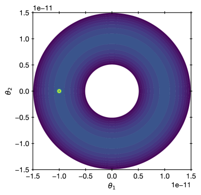
Figure 9: Likelihood contours of the diamond ring toy problem. A Gaussian shell (light green) is placed on a larger Gaussian shell. This is an example of a small spike on a slab. Note the small scales ($10^{-11}$) compared with the prior bounds $[-1,1]$.

The parameter space is two-dimensional, with $x$ and $y$ a priori uniform between $-1$ and $+1$. The likelihood is visualised in Figure 9. The distance $d$ from the ring radius $r$ is compared with the width $w$ using a Gaussian likelihood. The Gaussian shells make MCMC proposals difficult, as they have to slowly wander along the shell. Two Gaussian shells are added, with ratios $1:100$, making this a spike-and-slab problem. The posterior is very narrow compared with the prior range, requiring many NS iterations until the posterior is found.

We run NS with a fixed, relatively low number of live points ($N=100$). First, the number of MCMC steps in a LRPS method is tested. We choose HARM, with the number of steps per NS iteration ranging from 1 to 64. We also add the auto-tune method presented in Section 5.1.3. Figure 10 shows the run. In the top panel, the auto-tuning method rises twice, namely when the two shells are encountered and have to be navigated. Before, the number of steps could be tuned to low values, allowing it to be orders of magnitudes more efficient than using a safe number of steps throughout. The bottom panel of Figure 10 presents the accumulated integral estimate. The final $\log Z$ estimate between the NS runs vary stochastically in their final estimate, on a scale comparable to the uncertainty. The error bars are relatively large because of the small $N$, but are in acceptable ($<2\sigma$) agreement with the analytic value (dashed horizontal line). The accumulated $\log Z$ shows a plateau near iteration $5500$. This is the phase transition when the small “diamond” spike is being discovered on top of the larger ring (slab). If runs had stopped before, based on a fixed computing budget or because the live points appear similar, the additional probability would not have been discovered.

At the same time, the parameter space also becomes difficult to navigate along the thin ring. The small euclidean distances traversed cause the auto-tune method to increase its number of steps (grey curve rises in the top panel). The U test is presented in the middle panel. The curves vary mostly stochastically, not detecting strong deviations even for the shortest MCMC step numbers. These curves look substantially different, depending on what accumulation bandwidth is chosen (here: 1000 iterations), indicating that the insertion order does not see problems with the sampling. This agrees with the mutually consistent $\log Z$ estimates (error bars in bottom panel), which are usually very sensitive to incorrect LRPS sampling.

Taking these results together, one may want to run HARM with at least 4 steps until the likelihood corresponding to iteration 5000, and subsequently with 200 steps.

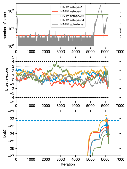
Figure 10: Number of MCMC steps. Five runs on the toy problem are shown using HARM (Hit-and-Run Monte Carlo) method. Top panel: Number of steps per new sample. This is varied in the auto-tuning method. Middle panel: z-score of the U test computed in a rolling window of 1000 iterations. Bottom panel: Integral estimates. Between iteration 5000 and 6000, a phase transition can be observed where initially the integral estimate plateaus and then rapidly increases again. The dashed line is the true value.

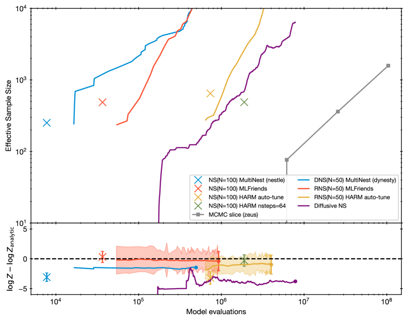
Figure 11: Efficiency comparison of different LRPS methods, some using Dynamic NS or Reactive NS. Top panel: Effective number of samples extracted (upper left is better than lower right). MCMC, after an initial phase of identifying the posterior, scales approximately linearly. MLFriends (orange) and auto-tuning HARM (green) show the steeper increase in samples per computation cost. Bottom panel: Integral estimate, relative to analytic value. The error bar and shaded ares show $1\sigma$ uncertainty estimates, when available.

The efficiency in extracting effective samples of various methods is compared in Figure 11. To avoid giving a strong geometric advantages to region-based methods, low $N$ are deliberately chosen. MultiNest and MLFriends perform similarly within a factor of three (blue, orange cross). As remarked above, HARM auto-tune (yellow cross) is substantially more efficient than HARM with a large, fixed number of steps per iterations (green cross).

With Dynamic Nested Sampling, started with $N=50$, and iteratively adding $50$ live points, dynesty can efficiently extract more and more effective samples (blue curve in Figure 11). The Reactive NS methods developed here are used with an agent that selects points based on posterior weights, and expands their parent nodes. This is applied to MLFriends and HARM auto-tune (red and yellow curves, respectively). Interestingly, the curve for MLFriends rises super-linearly with likelihood cost. MLFriends scales in this problem inversely with the number of live points. This is because the sampling region can be approximated better, leading to smaller rejection rates. Of course, this is only possible because of the low dimension of this problem. MLFriends scales better than MultiNest here, because the ellipsoid clustering is a poor description of the Gaussian shells. There are of course problems where the converse is true, such as L-shaped likelihood contours, where MultiNest substantially outperforms MLFriends. Interestingly, also HARM auto-tune scales steeply with likelihood evaluations. More live points mean the mean distance between them is smaller, therefore the number of steps needed to reach a new point is smaller.

The Diffusive Nested Sampler DNest4 shows approximately a linear scaling (purple curve in Figure 11). The number of likelihood evaluations needed is higher than for the other methods. For comparison, we also include a MCMC method, using the slice sampler zeus (Karamanis and Beutler, 2020). This shows a linear scaling (grey curve) after an initial phase where the posterior needs to be identified. The efficiency of extracting posterior samples in this case is substantially higher in NS methods, because the MCMC auto-correlation is exceptionally poor. The computational cost comparison in this problem is not representative of high-dimensional problems, where the ranking of methods may be different and even reversed.

The bottom panel of Figure 11 compares the integral estimates. Here, the MultiNest estimate is off, as it excludes the true value within its very small error bars. MLFriends and HARM methods agree with the analytic value within $2\sigma$. The dynamic and reactive nested sampling runs retain substantial uncertainties even with many likelihood evaluations. This is because new live points are not added to the initial phase of the run, causing the shrinkage estimates to remain uncertain. DNest4 initially shows convergence to the true value, but this trend is not improving later. DNest4 does not report uncertainties.

The MLFriends (for low-d) and HARM auto-tune (for low and high-d) methods appear promising. They are implemented in the UltraNest Python package, with support for massively parallel computing on clusters.

8 Summary

This review has surveyed the nested sampling literature across many subfields, and compiled proposed ideas and concepts. We have described the problem types nested sampling is suitable for, and laid out the practical difficulties implementations need to solve. To summarise:

1. Nested sampling is a practically useful algorithm for Bayesian model comparison and parameter inference. It globally explores the parameter space. This is important in problems with potentially complex, multi-modal likelihoods. The exploration can largely proceed unsupervised and without problem-specific tuning until a well-defined convergence point. Nested sampling has some limitations to scale to very high dimensional and highly informative problems.

2. This review highlighted the diversity of NS variants have been developed. These include: NS without any MCMC (such as MultiNest and MLFriends), using MCMC within NS, and running NS as a MCMC chain (Diffusive Nested Sampling). A relatively recent development is to integrate HMC more deeply, and adapting geometric random walk algorithms such as hit-and-run and slice sampling.

3. Diagnostics and visualisations of the quality and correctness of runs have improved substantially in the last few years.

9 Future research

Much of the literature is involved with the application of nested sampling to specific problems, evaluating its quality, and also proposing new NS variants and implementations. Beyond this, we see the need for systematic theoretical and practical evaluations in the future:

1. Investigating the theoretical foundations with an extended Sequential Monte Carlo framework seems particularly promising. Given that NS mutates only one particle, it should be investigated what theorems can be transferred to such an extended framework.

2. Systematic numerical comparisons of a wide range of problems across the PMDIT space are needed to judge the capabilities and limitations of NS variants, including the LRPS methods and their tuning parameters.

Appendix A On encoding prior distributions

The unit hypercube transformation, $u\rightarrow\theta$, is a way to encode priors by parametrising them in natural probability units, $u_{i}\in[0,1]$. In factorised priors, the transformation is achieved with inverse cumulative distribution functions, $\theta_{i}=F^{-1}(u_{i})$. It is convenient as constant-energy trajectories are straight, and sampling from geometrical shapes can be achieved without an additional rejection. For this reason, some (but not all) popular NS implementations let users specify priors via unit hypercube transformations, and in many examples demonstrate only factorised priors. This has lead some to believe that NS requires hypercubes and factorised priors. Here we clarify that neither is the case.

Firstly, NS can proceed as long as a LRPS method and a likelihood are defined. If the prior space is not $\mathbb{R}^{d}$, but arbitrary “objects”, a simple example includes Metropolis samplers that perturb the sample following the prior density. Indeed, such generic treatments are possible in DNest4 (Brewer and Foreman-Mackey, 2018). This includes allowing the dimensionality to vary, as demonstrated in Brewer (2014).

Secondly, we demonstrate two real-world cases where dependent priors can be encoded in NS with unit hypercube transformations. Consider a correlated Gaussian prior, defined by mean $\boldsymbol{\mu}$ and covariance $\boldsymbol{\Sigma}$. The transform from a unit interval $u\in[0,1]$ to an uncorrelated, standard normal prior can be encoded through inverse cumulative distribution functions, $z_{i}=F^{-1}(u_{i})$. Secondly, the transform from a standard normal prior to a general Gaussian is performed with an affine transform, $\theta=\boldsymbol{A}z+\mu$, where $\boldsymbol{\Sigma}=\boldsymbol{A}\boldsymbol{A}^{T}$. Therefore, a correlated sample is obtained. This approach is not limited to multi-variate Gaussians. For example, a Student-t would work the same and can receive a degrees of freedom parameter. The generalisation of this approach are copula models (e.g., Nelsen, 2007).

As a general approach, it can be useful to first transform one variable, and then iteratively consider the conditional cumulative distribution of the next given the previous. This iterative conditional approach can also be applied if a non-analytic prior is only available as a multi-dimensional histogram or samples $s$.

Often, procedures from random number generation can be adapted. As an example, consider the problem of encoding fractions into the parametrisation. This occurs for example when trying to fit for the elemental abundance of some physical object, where the relative fractions must sum to one. In some cases, it may be worthwhile to fit for an absolute parameter, such as the total mass of that element, if that is closer to the observable, and obtain fractions from the posterior. However, this requires placing priors on the masses, which may be difficult. Lets therefore assume we want to assume that the fractions each receive uniform priors, but simultaneously must sum to unity. The appropriate distribution for this scenario is the flat Dirichlet distribution with $\alpha=1$. To obtain prior samples using a hypercube transformation, we obtain independent gamma variables $z_{i}\sim\mathrm{Gamma}(\alpha,1)$, i.e., $z_{i}=-\log u_{i}$, and obtain the fraction variables as $\theta_{i}=z_{i}/\sum_{i}z_{i}$. More sophisticated transformations may be chosen to improve LRPS efficiency (Betancourt, 2012).

We comment in passing that state-of-the-art HMC frameworks use similar transformations internally to avoid trajectories exceeding the prior support (Carpenter et al., 2017).

Appendix B Ellipsoidal sampling efficiency for ellipsoidal likelihoods

The computational cost of ellipsoidal nested sampling (Mukherjee, Parkinson and Liddle, 2006) in the case of ellipsoidal likelihood contours is numerically explored, following Allison and Dunkley (2014). Different to their fixed enlargement treatment, here we determine the enlargement needed for rejection sampling: We generate $N$ points from a hypersphere of dimension $d$. In a bootstrapping scheme, we randomly leave points out (Buchner, 2016) and compute from the remainder a sample covariance matrix. This is used to construct an ellipsoid, enlarged by the factor needed to recover all left-out points. This is repeated 50 times, and the largest enlargement factor stored. The ellipsoid volume ratio of the original sphere and the constructed ellipsoid gives the acceptance rate of ellipsoidal rejection sampling.

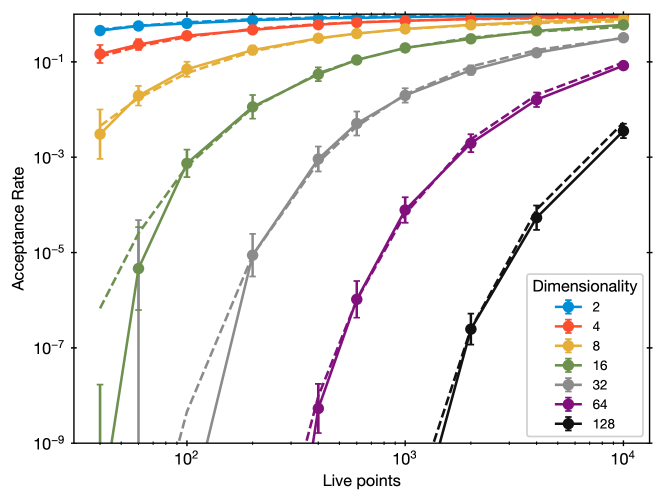
Figure 12: Acceptance rate for ellipsoidal rejection sampling. These measure the inverse excess volume of the constructed ellipsoids to reliably sample the posterior. More live points lead to tighter ellipsoids and higher acceptance rates. Increasing the number of dimensions decreases the acceptance rate. The dashed curve shows the empirical approximation of eq. 3, with the same colours as the data points for each dimensionality.

Figure 12 presents the acceptance rate $\alpha$ as a function of $N$ and $d$. Error bars indicate the standard deviation across 40 independently computed $\alpha$. Figure 12 shows that the acceptance rate increases with the number of live points $N$, but decreases with dimensionality. Figure 12 suggests that acceptance rates of $50\%$ can be maintained when $d$ doubles if $N$ increases five-fold. When $N$ is much smaller than the dimensionality, this method breaks down dramatically. The data points can be empirically described (dashed curves) by the following formula:

$$\alpha=\left(1.07-\log d^{1/3}\right)\times\exp\left\{-\left(\frac{6.83\times d^{1.9}}{N}\right)^{3/4}\right\}$$ (5)

The first term decreases the acceptance rate only mildly with dimensionality, and is therefore neglected in the cost scaling computations. The average cost, i.e., the number of model evaluations needed, is $C_{\mathrm{ell}}=1/\alpha$.

References

- Albert (2020) {barticle}[author] \bauthor\bsnmAlbert, \bfnmJoshua G.\binitsJ. G. (\byear2020). \btitleJAXNS: a high-performance nested sampling package based on JAX. \bjournalarXiv e-prints \bpagesarXiv:2012.15286. \endbibitem
- Allison and Dunkley (2014) {barticle}[author] \bauthor\bsnmAllison, \bfnmR.\binitsR. and \bauthor\bsnmDunkley, \bfnmJ.\binitsJ. (\byear2014). \btitleComparison of sampling techniques for Bayesian parameter estimation. \bjournalMNRAS \bvolume437 \bpages3918-3928. \bdoi10.1093/mnras/stt2190 \endbibitem
- Baldock et al. (2016) {barticle}[author] \bauthor\bsnmBaldock, \bfnmR. J. N.\binitsR. J. N., \bauthor\bsnmPártay, \bfnmL. B.\binitsL. B., \bauthor\bsnmBartók, \bfnmA. P.\binitsA. P., \bauthor\bsnmPayne, \bfnmM. C.\binitsM. C. and \bauthor\bsnmCsányi, \bfnmG.\binitsG. (\byear2016). \btitleDetermining pressure-temperature phase diagrams of materials. \bjournalPhys. Rev. B \bvolume93 \bpages174108. \bdoi10.1103/PhysRevB.93.174108 \endbibitem
- Baldock et al. (2017) {barticle}[author] \bauthor\bsnmBaldock, \bfnmRobert JN\binitsR. J., \bauthor\bsnmBernstein, \bfnmNoam\binitsN., \bauthor\bsnmSalerno, \bfnmK Michael\binitsK. M., \bauthor\bsnmPártay, \bfnmLívia B\binitsL. B. and \bauthor\bsnmCsányi, \bfnmGábor\binitsG. (\byear2017). \btitleConstant-pressure nested sampling with atomistic dynamics. \bjournalPhysical Review E \bvolume96 \bpages043311. \endbibitem
- Barbary (2016) {bmisc}[author] \bauthor\bsnmBarbary, \bfnmKyle\binitsK. (\byear2016). \btitlenestle v0.2.0. \bhowpublishedhttps://github.com/kbarbary/nestle/. \endbibitem
- Beaton and Xiang (2017) {barticle}[author] \bauthor\bsnmBeaton, \bfnmDouglas\binitsD. and \bauthor\bsnmXiang, \bfnmNing\binitsN. (\byear2017). \btitleRoom acoustic modal analysis using Bayesian inference a. \bjournalThe Journal of the Acoustical Society of America \bvolume141 \bpages4480–4493. \endbibitem
- Betancourt (2011) {binproceedings}[author] \bauthor\bsnmBetancourt, \bfnmM.\binitsM. (\byear2011). \btitleNested Sampling with Constrained Hamiltonian Monte Carlo. In \bbooktitleAmerican Institute of Physics Conference Series (\beditor\bfnmA.\binitsA. \bsnmMohammad-Djafari, \beditor\bfnmJ. F.\binitsJ. F. \bsnmBercher and \beditor\bfnmP.\binitsP. \bsnmBessiére, eds.). \bseriesAmerican Institute of Physics Conference Series \bvolume1305 \bpages165-172. \bdoi10.1063/1.3573613 \endbibitem
- Betancourt (2012) {binproceedings}[author] \bauthor\bsnmBetancourt, \bfnmMichael\binitsM. (\byear2012). \btitleCruising the simplex: Hamiltonian Monte Carlo and the Dirichlet distribution. In \bbooktitleBayesian Inference and Maximum Entropy Methods in Science and Engineering: 31st International Workshop on Bayesian Inference and Maximum Entropy Methods in Science and Engineering (\beditor\bfnmPhilip\binitsP. \bsnmGoyal, \beditor\bfnmAdom\binitsA. \bsnmGiffin, \beditor\bfnmKevin H.\binitsK. H. \bsnmKnuth and \beditor\bfnmEdward\binitsE. \bsnmVrscay, eds.). \bseriesAmerican Institute of Physics Conference Series \bvolume1443 \bpages157-164. \bdoi10.1063/1.3703631 \endbibitem
- Betancourt (2017) {barticle}[author] \bauthor\bsnmBetancourt, \bfnmMichael\binitsM. (\byear2017). \btitleA Conceptual Introduction to Hamiltonian Monte Carlo. \bjournalarXiv e-prints \bpagesarXiv:1701.02434. \endbibitem
- Birge, Chang and Polson (2012) {barticle}[author] \bauthor\bsnmBirge, \bfnmJohn R.\binitsJ. R., \bauthor\bsnmChang, \bfnmChanggee\binitsC. and \bauthor\bsnmPolson, \bfnmNicholas G.\binitsN. G. (\byear2012). \btitleSplit Sampling: Expectations, Normalisation and Rare Events. \bjournalarXiv e-prints \bpagesarXiv:1212.0534. \endbibitem
- Brewer (2014) {barticle}[author] \bauthor\bsnmBrewer, \bfnmBrendon J.\binitsB. J. (\byear2014). \btitleInference for Trans-dimensional Bayesian Models with Diffusive Nested Sampling. \bjournalarXiv e-prints \bpagesarXiv:1411.3921. \endbibitem
- Brewer (2017) {barticle}[author] \bauthor\bsnmBrewer, \bfnmB. J.\binitsB. J. (\byear2017). \btitleComputing Entropies With Nested Sampling. \bjournalArXiv e-prints. \endbibitem
- Brewer and Foreman-Mackey (2018) {barticle}[author] \bauthor\bsnmBrewer, \bfnmBrendon J.\binitsB. J. and \bauthor\bsnmForeman-Mackey, \bfnmDaniel\binitsD. (\byear2018). \btitleDNest4: Diffusive Nested Sampling in C++ and Python. \bjournalJournal of Statistical Software, Articles \bvolume86 \bpages1–33. \bdoi10.18637/jss.v086.i07 \endbibitem
- Brewer, Pártay and Csányi (2011) {barticle}[author] \bauthor\bsnmBrewer, \bfnmBrendon J\binitsB. J., \bauthor\bsnmPártay, \bfnmLivia B\binitsL. B. and \bauthor\bsnmCsányi, \bfnmGábor\binitsG. (\byear2011). \btitleDiffusive nested sampling. \bjournalArXiv e-prints \bvolume21 \bpages649–656. \endbibitem
- Buchner (2014) {barticle}[author] \bauthor\bsnmBuchner, \bfnmJohannes\binitsJ. (\byear2014). \btitleA statistical test for Nested Sampling algorithms. \bjournalStatistics and Computing \bpages1-10. \bdoi10.1007/s11222-014-9512-y \endbibitem
- Buchner (2015) {bmisc}[author] \bauthor\bsnmBuchner, \bfnmJohannes\binitsJ. (\byear2015). \btitleRMultiNest. \bhowpublishedhttps://github.com/JohannesBuchner/RMultiNest. \endbibitem
- Buchner (2016) {barticle}[author] \bauthor\bsnmBuchner, \bfnmJohannes\binitsJ. (\byear2016). \btitleA statistical test for Nested Sampling algorithms. \bjournalStatistics and Computing \bvolume26 \bpages383-392. \bdoi10.1007/s11222-014-9512-y \endbibitem
- Buchner (2019) {barticle}[author] \bauthor\bsnmBuchner, \bfnmJohannes\binitsJ. (\byear2019). \btitleCollaborative Nested Sampling: Big Data versus Complex Physical Models. \bjournalPASP \bvolume131 \bpages108005. \bdoi10.1088/1538-3873/aae7fc \endbibitem
- Buchner et al. (2014) {barticle}[author] \bauthor\bsnmBuchner, \bfnmJ.\binitsJ., \bauthor\bsnmGeorgakakis, \bfnmA.\binitsA., \bauthor\bsnmNandra, \bfnmK.\binitsK., \bauthor\bsnmHsu, \bfnmL.\binitsL., \bauthor\bsnmRangel, \bfnmC.\binitsC., \bauthor\bsnmBrightman, \bfnmM.\binitsM., \bauthor\bsnmMerloni, \bfnmA.\binitsA., \bauthor\bsnmSalvato, \bfnmM.\binitsM., \bauthor\bsnmDonley, \bfnmJ.\binitsJ. and \bauthor\bsnmKocevski, \bfnmD.\binitsD. (\byear2014). \btitleX-ray spectral modelling of the AGN obscuring region in the CDFS: Bayesian model selection and catalogue. \bjournalA&A \bvolume564 \bpagesA125. \bdoi10.1051/0004-6361/201322971 \endbibitem
- Burkoff et al. (2012) {barticle}[author] \bauthor\bsnmBurkoff, \bfnmNikolas S\binitsN. S., \bauthor\bsnmVárnai, \bfnmCsilla\binitsC., \bauthor\bsnmWells, \bfnmStephen A\binitsS. A. and \bauthor\bsnmWild, \bfnmDavid L\binitsD. L. (\byear2012). \btitleExploring the energy landscapes of protein folding simulations with Bayesian computation. \bjournalBiophysical journal \bvolume102 \bpages878–886. \endbibitem
- Cameron and Pettitt (2014) {barticle}[author] \bauthor\bsnmCameron, \bfnmEwan\binitsE. and \bauthor\bsnmPettitt, \bfnmAnthony\binitsA. (\byear2014). \btitleRecursive pathways to marginal likelihood estimation with prior-sensitivity analysis. \bjournalStatistical Science \bvolume29 \bpages397–419. \endbibitem
- Carpenter et al. (2017) {barticle}[author] \bauthor\bsnmCarpenter, \bfnmBob\binitsB., \bauthor\bsnmGelman, \bfnmAndrew\binitsA., \bauthor\bsnmHoffman, \bfnmMatthew D\binitsM. D., \bauthor\bsnmLee, \bfnmDaniel\binitsD., \bauthor\bsnmGoodrich, \bfnmBen\binitsB., \bauthor\bsnmBetancourt, \bfnmMichael\binitsM., \bauthor\bsnmBrubaker, \bfnmMarcus\binitsM., \bauthor\bsnmGuo, \bfnmJiqiang\binitsJ., \bauthor\bsnmLi, \bfnmPeter\binitsP. and \bauthor\bsnmRiddell, \bfnmAllen\binitsA. (\byear2017). \btitleStan: A probabilistic programming language. \bjournalJournal of statistical software \bvolume76 \bpages1–32. \endbibitem
- Chopin and Robert (2007a) {barticle}[author] \bauthor\bsnmChopin, \bfnmN\binitsN. and \bauthor\bsnmRobert, \bfnmC\binitsC. (\byear2007a). \btitleComments on Nested Sampling by John Skilling. \bjournalBayesian Statistics \bvolume8 \bpages491–524. \endbibitem
- Chopin and Robert (2007b) {btechreport}[author] \bauthor\bsnmChopin, \bfnmNicolas\binitsN. and \bauthor\bsnmRobert, \bfnmChristian\binitsC. (\byear2007b). \btitleContemplating evidence: properties, extensions of, and alternatives to nested sampling \btypeTechnical Report, \bpublisherTechnical Report 2007-46, CEREMADE, Université Paris Dauphine. \endbibitem
- Chopin and Robert (2008) {barticle}[author] \bauthor\bsnmChopin, \bfnmN.\binitsN. and \bauthor\bsnmRobert, \bfnmC.\binitsC. (\byear2008). \btitleProperties of Nested Sampling. \bjournalArXiv e-prints. \endbibitem
- Chopin and Robert (2010) {barticle}[author] \bauthor\bsnmChopin, \bfnmNicolas\binitsN. and \bauthor\bsnmRobert, \bfnmChristian P.\binitsC. P. (\byear2010). \btitleProperties of nested sampling. \bjournalBiometrika. \bdoi10.1093/biomet/asq021 \endbibitem
- Collins et al. (2013) {barticle}[author] \bauthor\bsnmCollins, \bfnmB.\binitsB., \bauthor\bsnmKousha, \bfnmT.\binitsT., \bauthor\bsnmKulik, \bfnmR.\binitsR., \bauthor\bsnmSzarek, \bfnmT.\binitsT. and \bauthor\bsnmŻyczkowski, \bfnmK.\binitsK. (\byear2013). \btitleThe accessibility of convex bodies and derandomization of the hit and run algorithm. \bjournalArXiv e-prints. \endbibitem
- Corsaro and De Ridder (2014) {barticle}[author] \bauthor\bsnmCorsaro, \bfnmE.\binitsE. and \bauthor\bsnmDe Ridder, \bfnmJ.\binitsJ. (\byear2014). \btitleDIAMONDS: A new Bayesian nested sampling tool. Application to peak bagging of solar-like oscillations. \bjournalA&A \bvolume571 \bpagesA71. \bdoi10.1051/0004-6361/201424181 \endbibitem
- Evans (2007) {barticle}[author] \bauthor\bsnmEvans, \bfnmM\binitsM. (\byear2007). \btitleDiscussion of nested sampling for Bayesian computations by John Skilling. \bjournalBayesian Statistics \bvolume8 \bpages491–524. \endbibitem
- Feroz and Hobson (2008) {barticle}[author] \bauthor\bsnmFeroz, \bfnmF.\binitsF. and \bauthor\bsnmHobson, \bfnmM. P.\binitsM. P. (\byear2008). \btitleMultimodal nested sampling: an efficient and robust alternative to Markov Chain Monte Carlo methods for astronomical data analyses. \bjournalMNRAS \bvolume384 \bpages449-463. \bdoi10.1111/j.1365-2966.2007.12353.x \endbibitem
- Feroz, Hobson and Bridges (2009) {barticle}[author] \bauthor\bsnmFeroz, \bfnmF.\binitsF., \bauthor\bsnmHobson, \bfnmM. P.\binitsM. P. and \bauthor\bsnmBridges, \bfnmM.\binitsM. (\byear2009). \btitleMULTINEST: an efficient and robust Bayesian inference tool for cosmology and particle physics. \bjournalMNRAS \bvolume398 \bpages1601-1614. \bdoi10.1111/j.1365-2966.2009.14548.x \endbibitem
- Feroz et al. (2013) {barticle}[author] \bauthor\bsnmFeroz, \bfnmF.\binitsF., \bauthor\bsnmHobson, \bfnmM. P.\binitsM. P., \bauthor\bsnmCameron, \bfnmE.\binitsE. and \bauthor\bsnmPettitt, \bfnmA. N.\binitsA. N. (\byear2013). \btitleImportance Nested Sampling and the MultiNest Algorithm. \bjournalArXiv e-prints. \endbibitem
- Fowlie, Handley and Su (2020) {barticle}[author] \bauthor\bsnmFowlie, \bfnmAndrew\binitsA., \bauthor\bsnmHandley, \bfnmWill\binitsW. and \bauthor\bsnmSu, \bfnmLiangliang\binitsL. (\byear2020). \btitleNested sampling cross-checks using order statistics. \bjournalarXiv e-prints \bpagesarXiv:2006.03371. \endbibitem
- Fowlie, Handley and Su (2021) {barticle}[author] \bauthor\bsnmFowlie, \bfnmAndrew\binitsA., \bauthor\bsnmHandley, \bfnmWill\binitsW. and \bauthor\bsnmSu, \bfnmLiangliang\binitsL. (\byear2021). \btitleNested sampling with plateaus. \bjournalMNRAS \bvolume503 \bpages1199-1205. \bdoi10.1093/mnras/stab590 \endbibitem
- Gervino, Mana and Palmisano (2016) {barticle}[author] \bauthor\bsnmGervino, \bfnmGianpiero\binitsG., \bauthor\bsnmMana, \bfnmGiovanni\binitsG. and \bauthor\bsnmPalmisano, \bfnmCarlo\binitsC. (\byear2016). \btitleThe ellipsoidal nested sampling and the expression of the model uncertainty in measurements. \bjournalInternational Journal of Modern Physics B \bpages1541002. \endbibitem
- Goggans, Henderson and Cao (2014) {barticle}[author] \bauthor\bsnmGoggans, \bfnmPaul M.\binitsP. M., \bauthor\bsnmHenderson, \bfnmR. Wesley\binitsR. W. and \bauthor\bsnmCao, \bfnmLei\binitsL. (\byear2014). \btitleDesign-as-inference: Probability-based design of intermodal transportation networks. \bjournalAIP Conference Proceedings \bvolume1636 \bpages145-150. \bdoi10.1063/1.4903724 \endbibitem
- Goodman and Weare (2010) {barticle}[author] \bauthor\bsnmGoodman, \bfnmJ.\binitsJ. and \bauthor\bsnmWeare, \bfnmJ.\binitsJ. (\byear2010). \btitleEnsemble samplers with affine invariance. \bjournalCommunications in Applied Mathematics and Computational Science, Vol. 5, No. 1, p. 65-80, 2010 \bvolume5 \bpages65-80. \bdoi10.2140/camcos.2010.5.65 \endbibitem
- Graff et al. (2012) {barticle}[author] \bauthor\bsnmGraff, \bfnmP.\binitsP., \bauthor\bsnmFeroz, \bfnmF.\binitsF., \bauthor\bsnmHobson, \bfnmM. P.\binitsM. P. and \bauthor\bsnmLasenby, \bfnmA.\binitsA. (\byear2012). \btitleBAMBI: blind accelerated multimodal Bayesian inference. \bjournalMNRAS \bvolume421 \bpages169-180. \bdoi10.1111/j.1365-2966.2011.20288.x \endbibitem
- Griffiths and Wales (2019) {barticle}[author] \bauthor\bsnmGriffiths, \bfnmMatthew\binitsM. and \bauthor\bsnmWales, \bfnmDavid J\binitsD. J. (\byear2019). \btitleNested basin-sampling. \bjournalJournal of Chemical Theory and Computation \bvolume15 \bpages6865–6881. \endbibitem
- Guyader, Hengartner and Matzner-Løber (2011) {barticle}[author] \bauthor\bsnmGuyader, \bfnmArnaud\binitsA., \bauthor\bsnmHengartner, \bfnmNicolas\binitsN. and \bauthor\bsnmMatzner-Løber, \bfnmEric\binitsE. (\byear2011). \btitleSimulation and estimation of extreme quantiles and extreme probabilities. \bjournalApplied Mathematics & Optimization \bvolume64 \bpages171–196. \endbibitem
- Habeck (2015) {binproceedings}[author] \bauthor\bsnmHabeck, \bfnmM.\binitsM. (\byear2015). \btitleNested sampling with demons. In \bbooktitleAmerican Institute of Physics Conference Series. \bseriesAmerican Institute of Physics Conference Series \bvolume1641 \bpages121-129. \bdoi10.1063/1.4905971 \endbibitem
- Handley, Hobson and Lasenby (2015a) {barticle}[author] \bauthor\bsnmHandley, \bfnmW. J.\binitsW. J., \bauthor\bsnmHobson, \bfnmM. P.\binitsM. P. and \bauthor\bsnmLasenby, \bfnmA. N.\binitsA. N. (\byear2015a). \btitlePOLYCHORD: next-generation nested sampling. \bjournalMNRAS \bvolume453 \bpages4384-4398. \bdoi10.1093/mnras/stv1911 \endbibitem
- Handley, Hobson and Lasenby (2015b) {barticle}[author] \bauthor\bsnmHandley, \bfnmW. J.\binitsW. J., \bauthor\bsnmHobson, \bfnmM. P.\binitsM. P. and \bauthor\bsnmLasenby, \bfnmA. N.\binitsA. N. (\byear2015b). \btitlePOLYCHORD: nested sampling for cosmology. \bjournalMNRAS \bvolume450 \bpagesL61-L65. \bdoi10.1093/mnrasl/slv047 \endbibitem
- Henderson and Goggans (2014) {binproceedings}[author] \bauthor\bsnmHenderson, \bfnmR Wesley\binitsR. W. and \bauthor\bsnmGoggans, \bfnmPaul M\binitsP. M. (\byear2014). \btitleParallelized nested sampling. In \bbooktitleAIP Conference Proceedings \bvolume1636 \bpages100–105. \bpublisherAIP. \endbibitem
- Henderson, Goggans and Cao (2017) {barticle}[author] \bauthor\bsnmHenderson, \bfnmR. Wesley\binitsR. W., \bauthor\bsnmGoggans, \bfnmPaul M.\binitsP. M. and \bauthor\bsnmCao, \bfnmLei\binitsL. (\byear2017). \btitleCombined-chain nested sampling for efficient Bayesian model comparison. \bjournalDigital Signal Processing \bvolume70 \bpages84 - 93. \bdoihttp://dx.doi.org/10.1016/j.dsp.2017.07.021 \endbibitem
- Higson et al. (2017) {barticle}[author] \bauthor\bsnmHigson, \bfnmE.\binitsE., \bauthor\bsnmHandley, \bfnmW.\binitsW., \bauthor\bsnmHobson, \bfnmM.\binitsM. and \bauthor\bsnmLasenby, \bfnmA.\binitsA. (\byear2017). \btitleDynamic nested sampling: an improved algorithm for parameter estimation and evidence calculation. \bjournalArXiv e-prints. \endbibitem
- Higson et al. (2018) {barticle}[author] \bauthor\bsnmHigson, \bfnmEdward\binitsE., \bauthor\bsnmHandley, \bfnmWill\binitsW., \bauthor\bsnmHobson, \bfnmMike\binitsM. and \bauthor\bsnmLasenby, \bfnmAnthony\binitsA. (\byear2018). \btitleSampling Errors in Nested Sampling Parameter Estimation. \bjournalBayesian Analysis \bvolume13 \bpages873-896. \endbibitem
- Higson et al. (2019) {barticle}[author] \bauthor\bsnmHigson, \bfnmEdward\binitsE., \bauthor\bsnmHandley, \bfnmWill\binitsW., \bauthor\bsnmHobson, \bfnmMichael\binitsM. and \bauthor\bsnmLasenby, \bfnmAnthony\binitsA. (\byear2019). \btitleNESTCHECK: diagnostic tests for nested sampling calculations. \bjournalMNRAS \bvolume483 \bpages2044-2056. \bdoi10.1093/mnras/sty3090 \endbibitem
- Hoffman and Gelman (2014) {barticle}[author] \bauthor\bsnmHoffman, \bfnmMatthew D\binitsM. D. and \bauthor\bsnmGelman, \bfnmAndrew\binitsA. (\byear2014). \btitleThe No-U-turn sampler: adaptively setting path lengths in Hamiltonian Monte Carlo. \bjournalJournal of Machine Learning Research \bvolume15 \bpages1593–1623. \endbibitem
- Huber and Schott (2010) {barticle}[author] \bauthor\bsnmHuber, \bfnmMark\binitsM. and \bauthor\bsnmSchott, \bfnmSarah\binitsS. (\byear2010). \btitleUsing TPA for Bayesian inference. \bjournalBayesian Statistics 9. \endbibitem
- Huijser, Goodman and Brewer (2015) {barticle}[author] \bauthor\bsnmHuijser, \bfnmDavid\binitsD., \bauthor\bsnmGoodman, \bfnmJesse\binitsJ. and \bauthor\bsnmBrewer, \bfnmBrendon J.\binitsB. J. (\byear2015). \btitleProperties of the Affine Invariant Ensemble Sampler in high dimensions. \bjournalarXiv e-prints \bpagesarXiv:1509.02230. \endbibitem
- Jarvis and Patrick (1973) {barticle}[author] \bauthor\bsnmJarvis, \bfnmRaymond Austin\binitsR. A. and \bauthor\bsnmPatrick, \bfnmEdward A\binitsE. A. (\byear1973). \btitleClustering using a similarity measure based on shared near neighbors. \bjournalIEEE Transactions on computers \bvolume100 \bpages1025–1034. \endbibitem
- Javid (2019) {barticle}[author] \bauthor\bsnmJavid, \bfnmKamran\binitsK. (\byear2019). \btitleNested sampling on non-trivial geometries. \bjournalarXiv e-prints \bpagesarXiv:1905.09110. \endbibitem
- Javid et al. (2020) {barticle}[author] \bauthor\bsnmJavid, \bfnmKamran\binitsK., \bauthor\bsnmHandley, \bfnmWill\binitsW., \bauthor\bsnmHobson, \bfnmMike\binitsM. and \bauthor\bsnmLasenby, \bfnmAnthony\binitsA. (\byear2020). \btitleCompromise-free Bayesian neural networks. \bjournalarXiv e-prints \bpagesarXiv:2004.12211. \endbibitem
- Jeffreys (1998) {barticle}[author] \bauthor\bsnmJeffreys, \bfnmH.\binitsH. (\byear1998). \btitleThe Theory of probability. \bjournalInternational series of monographs on physics. \endbibitem
- Karamanis and Beutler (2020) {barticle}[author] \bauthor\bsnmKaramanis, \bfnmMinas\binitsM. and \bauthor\bsnmBeutler, \bfnmFlorian\binitsF. (\byear2020). \btitleEnsemble Slice Sampling. \bjournalarXiv e-prints \bpagesarXiv:2002.06212. \endbibitem
- Kass and Raftery (1995) {barticle}[author] \bauthor\bsnmKass, \bfnmRobert E.\binitsR. E. and \bauthor\bsnmRaftery, \bfnmAdrian E.\binitsA. E. (\byear1995). \btitleBayes Factors. \bjournalJournal of the American Statistical Association \bvolume90 \bpages773-795. \bdoi10.1080/01621459.1995.10476572 \endbibitem
- Keeton (2011) {barticle}[author] \bauthor\bsnmKeeton, \bfnmC. R.\binitsC. R. (\byear2011). \btitleOn statistical uncertainty in nested sampling. \bjournalMNRAS \bvolume414 \bpages1418-1426. \bdoi10.1111/j.1365-2966.2011.18474.x \endbibitem
- Khanarian and Alvarez (2013) {bunpublished}[author] \bauthor\bsnmKhanarian, \bfnmMichael\binitsM. and \bauthor\bsnmAlvarez, \bfnmDavid\binitsD. (\byear2013). \btitleNests and Tootsie Pops: Bayesian Sampling with Monte Carlo. \endbibitem
- Kiatsupaibul, Smith and Zabinsky (2011) {barticle}[author] \bauthor\bsnmKiatsupaibul, \bfnmSeksan\binitsS., \bauthor\bsnmSmith, \bfnmRobert L.\binitsR. L. and \bauthor\bsnmZabinsky, \bfnmZelda B.\binitsZ. B. (\byear2011). \btitleAn Analysis of a Variation of Hit-and-run for Uniform Sampling from General Regions. \bjournalACM Trans. Model. Comput. Simul. \bvolume21 \bpages16:1–16:11. \bdoi10.1145/1921598.1921600 \endbibitem
- Kirkpatrick, Gelatt and Vecchi (1983) {barticle}[author] \bauthor\bsnmKirkpatrick, \bfnmS.\binitsS., \bauthor\bsnmGelatt, \bfnmC. D.\binitsC. D. and \bauthor\bsnmVecchi, \bfnmM. P.\binitsM. P. (\byear1983). \btitleOptimization by Simulated Annealing. \bjournalScience \bvolume220 \bpages671-680. \bdoi10.1126/science.220.4598.671 \endbibitem
- Liu et al. (2016) {barticle}[author] \bauthor\bsnmLiu, \bfnmPeigui\binitsP., \bauthor\bsnmElshall, \bfnmAhmed S\binitsA. S., \bauthor\bsnmYe, \bfnmMing\binitsM., \bauthor\bsnmBeerli, \bfnmPeter\binitsP., \bauthor\bsnmZeng, \bfnmXiankui\binitsX., \bauthor\bsnmLu, \bfnmDan\binitsD. and \bauthor\bsnmTao, \bfnmYuezan\binitsY. (\byear2016). \btitleEvaluating marginal likelihood with thermodynamic integration method and comparison with several other numerical methods. \bjournalWater Resources Research \bvolume52 \bpages734–758. \endbibitem
- Malakar and Knuth (2011) {binproceedings}[author] \bauthor\bsnmMalakar, \bfnmN. K.\binitsN. K. and \bauthor\bsnmKnuth, \bfnmK. H.\binitsK. H. (\byear2011). \btitleEntropy-Based Search Algorithm for Experimental Design. In \bbooktitleAmerican Institute of Physics Conference Series (\beditor\bfnmA.\binitsA. \bsnmMohammad-Djafari, \beditor\bfnmJ. F.\binitsJ. F. \bsnmBercher and \beditor\bfnmP.\binitsP. \bsnmBessiére, eds.). \bseriesAmerican Institute of Physics Conference Series \bvolume1305 \bpages157-164. \bdoi10.1063/1.3573612 \endbibitem
- Mann and Whitney (1947) {barticle}[author] \bauthor\bsnmMann, \bfnmH. B.\binitsH. B. and \bauthor\bsnmWhitney, \bfnmD. R.\binitsD. R. (\byear1947). \btitleOn a Test of Whether one of Two Random Variables is Stochastically Larger than the Other. \bjournalAnn. Math. Statist. \bvolume18 \bpages50–60. \bdoi10.1214/aoms/1177730491 \endbibitem
- Martiniani et al. (2014) {barticle}[author] \bauthor\bsnmMartiniani, \bfnmS.\binitsS., \bauthor\bsnmStevenson, \bfnmJ. D.\binitsJ. D., \bauthor\bsnmWales, \bfnmD. J.\binitsD. J. and \bauthor\bsnmFrenkel, \bfnmD.\binitsD. (\byear2014). \btitleSuperposition Enhanced Nested Sampling. \bjournalPhysical Review X \bvolume4 \bpages031034. \bdoi10.1103/PhysRevX.4.031034 \endbibitem
- Mikelson and Khammash (2020) {barticle}[author] \bauthor\bsnmMikelson, \bfnmJan\binitsJ. and \bauthor\bsnmKhammash, \bfnmMustafa\binitsM. (\byear2020). \btitleLikelihood-free nested sampling for parameter inference of biochemical reaction networks. \bjournalPLoS Computational Biology \bvolume16 \bpagese1008264. \bdoi10.1371/journal.pcbi.1008264 \endbibitem
- Möller et al. (2013) {barticle}[author] \bauthor\bsnmMöller, \bfnmT.\binitsT., \bauthor\bsnmBernst, \bfnmI.\binitsI., \bauthor\bsnmPanoglou, \bfnmD.\binitsD., \bauthor\bsnmMuders, \bfnmD.\binitsD., \bauthor\bsnmOssenkopf, \bfnmV.\binitsV., \bauthor\bsnmRöllig, \bfnmM.\binitsM. and \bauthor\bsnmSchilke, \bfnmP.\binitsP. (\byear2013). \btitleModeling and Analysis Generic Interface for eXternal numerical codes (MAGIX). \bjournalA&A \bvolume549 \bpagesA21. \bdoi10.1051/0004-6361/201220063 \endbibitem
- Moss (2020) {barticle}[author] \bauthor\bsnmMoss, \bfnmAdam\binitsA. (\byear2020). \btitleAccelerated Bayesian inference using deep learning. \bjournalMNRAS \bvolume496 \bpages328-338. \bdoi10.1093/mnras/staa1469 \endbibitem