Leveraging Expert Consistency
to Improve Algorithmic Decision Support

Abstract

Machine learning (ML) is increasingly being used to support high-stakes decisions, a trend owed in part to its promise of superior predictive power relative to human assessment. However, there is frequently a gap between decision objectives and what is captured in the observed outcomes used as labels to train ML models. As a result, machine learning models may fail to capture important dimensions of decision criteria, hampering their utility for decision support. In this work, we explore the use of historical expert decisions as a rich—yet imperfect—source of information that is commonly available in organizational information systems, and show that it can be leveraged to bridge the gap between decision objectives and algorithm objectives. We consider the problem of estimating expert consistency indirectly when each case in the data is assessed by a single expert, and propose influence function-based methodology as a solution to this problem. We then incorporate the estimated expert consistency into a predictive model through a training-time label amalgamation approach. This approach allows ML models to learn from experts when there is inferred expert consistency, and from observed labels otherwise. We also propose alternative ways of leveraging inferred consistency via hybrid and deferral models. In our empirical evaluation, focused on the context of child maltreatment hotline screenings, we show that (1) there are high-risk cases whose risk is considered by the experts but not wholly captured in the target labels used to train a deployed model, and (2) the proposed approach significantly improves precision for these cases.

1 Introduction

Across domains, experts routinely and implicitly make predictions to inform decisions their job requires them to make. Recruiters assess the likelihood of a candidate succeeding at a job if hired, physicians predict the likelihood of neurological recovery of comatose patients when deciding whether to extend their life support, judges predict the likelihood of recidivism when considering bail, and child abuse hotline call workers assess the risk of harm to a child when deciding whether a hotline call should prompt an investigation. Increasingly, machine learning (ML) is being used to aid experts in those predictions. This is largely motivated by research that has shown ML and actuarial models can perform better at making predictions than humans (Meehl, 1954, Dawes et al., 1989, Grove et al., 2000). However, research showing the superior predictive power of machines often makes simplifying assumptions concerning the data used for training such models and their decision targets. In particular, it typically assumes that the observed outcome perfectly captures the decision objective. In practice, the properties of available data frequently limit what can be learned from the observed outcomes alone, undermining deployed performance of predictive algorithms and leading to deceptively optimistic evaluations.

Broadly speaking, predictive algorithms for decision support, which can range from simple logistic regression models to complex deep neural networks, leverage large amounts of data available in organizational information systems to estimate the likelihood of an observed outcome. A record of observed outcomes constitutes the labels available for training. In some cases, human assessments are used as labels in the absence of directly observed outcomes of interest. These are typically obtained through data annotation efforts that query multiple humans per case and assign a label based on consensus or majority votes (Zhang et al., 2016, McKinney et al., 2020). For example, radiological diagnostic tools are trained to predict radiologists’ diagnoses, and hate speech prediction tools are trained to predict human annotations. However, human knowledge is often discarded whenever an observed outcome is available. This practice is arguably driven by two main factors: (1) a belief that observed outcomes provide a more reliable source of information; and (2) the high cost of data annotation processes necessary to obtain multiple expert assessments per case.

However, informing high-stakes decisions using ML models trained to predict an observed outcome may have crucial shortcomings and pose several risks. A primary, albeit often neglected, issue is construct validity (Passi and Barocas, 2019, Mullainathan and Obermeyer, 2017). Decision objectives are typically complex, multi-faceted constructs, and observed outcomes are an imperfect proxy for these. For example, Obermeyer et al., (2019) describe a setting in which predicted healthcare costs are taken as a proxy for healthcare needs when prioritizing patients with complex health conditions for coordinated care management programs. The authors show that the choice of cost as a prediction target can exacerbate racial disparities in healthcare. In the US, the costs incurred by Black patients are often considerably lower than those of white patients with similar healthcare needs. Thus an algorithm trained to predict cost might erroneously prioritize healthier white patients over more ill Black patients.

Deploying decision support tools that optimize for narrowly circumscribed outcomes can also shift the criteria people use for making decisions (Green and Chen, 2021). Such drifts in decision criteria may be undesired and have detrimental consequences in many domains. Consider the deployment of predictive models in the context of child maltreatment hotlines—the focus of the empirical evaluation of our work—where risk assessment algorithms have been deployed to assist call workers in identifying high risk cases. Call workers receiving phone reports of child neglect or abuse are tasked with deciding which cases should be screened-in for further investigation by a social worker who visits the home. The deployment of risk assessment tools aims to inform this decision by providing estimates of risk based on multi-system administrative data related to the children and adults associated to a referral. The question central to the decision is whether the child is at risk. As a proxy for risk, the predictive models estimate the probability of an out-of-home placement of the child, i.e., the removal of the child from the home and placement into foster care. While this is an important indicator of risk, in many cases other types of intervention can be offered to reduce the risk to the child without separating the family. A shift in decision criteria to only prioritize cases where the end result is out-of-home placement could increase risk to children for whom other interventions can be effective, and yield an agency lacking a holistic approach and perceived as adversarial because it primarily investigates cases that will result in family separation.

For this and other reasons, recent work has emphasized the importance of problem formulation in the design of sociotechnical machine learning systems (Passi and Barocas, 2019, Jacobs and Wallach, 2021), but so far the conversation has primarily centered on the importance of selecting an appropriate proxy for the decision objective. There is currently a lack of technical approaches to provide practitioners with a toolkit that enables them to better approximate a construct of interest when no single variable constitutes a sufficiently good proxy. In this work, we propose to use expert consistency as a source of information to enrich the objective optimized for by an algorithm. Often, expert knowledge is sufficient to correctly and consistently assess a subset of cases, while being insufficient for assessing other cases. For instance, physicians may have an easy time diagnosing patients that exhibit certain well-known symptoms, while not having sufficient information to conclusively diagnose other patients. Similarly, healthcare professionals tasked with enrolling patients in special care programs may have an easy time identifying certain types of complex health needs (irrespective of their health spending), while having a hard time prioritizing among the rest of the population. In the child welfare setting, this could manifest as subsets of cases for which certain attributes of the family (e.g., history of substance abuse) warrant a house visit, even if an out-of-home visit is unlikely to be necessary. The premise of the approach proposed in this paper is simple: learn from experts’ decisions whenever they display certainty and consistency, and learn from the observed outcomes otherwise.

In addition to mitigating issues of construct validity, the proposed approach addresses other shortcomings of learning from observed outcomes alone. In particular, it provides a solution for a problem that cannot be addressed without incorporating other sources of information: the violation of the positivity assumption in the selective labels problem. In many domains, outcomes may only be observed when human experts make a certain decision, which is known as the selective labels problem (Lakkaraju et al., 2017). For instance, a diagnostic test result may only be available if a physician chooses to prescribe a test. Similarly, the outcome following a social worker’s home visit may only be observed if a call worker chooses to screen-in a call for investigation. While many statistical approaches have been proposed for addressing this type of sampling bias, these typically rely on the positivity assumption, which states that there is a non-negligible probability of observing an outcome for all instances in the domain of interest. This assumption is violated if experts consistently make the decision that censors the outcome for a subset of cases, which can easily happen when domain expertise allows them to confidently assess such a subset. In such settings, our proposed approach enables learning from such expertise as a pathway to address the violation of the positivity assumption.

Our work builds on a long history of research and practice that uses human consistency as a source of information. Popularized by Cohen’s Kappa Coefficient (Cohen, 1960, Umesh et al., 1989), inter-rater agreement is considered an indicator of reliability (Banerjee et al., 1999, Gwet et al., 2002). Unlike settings of crowd sourcing and data labeling, however, expert decisions stored in organizational information systems often only record decisions of a single expert per case. Moreover, which expert is assigned to each case may be non-random. For instance, which physician sees a patient is likely to depend on location, insurance coverage, and work schedules. Similarly, call workers assigned to weekends or night shifts may attend to very different calls than their colleagues.

Therefore, we first consider the problem of estimating expert consistency indirectly, when each case is assessed by a single expert, and assignment of experts to cases is non-random. The proposed influence function based method proceeds as follows: a predictive model $\hat{f}_{h}$ is trained to predict the historical expert decisions, and influence functions are used to estimate each expert’s influence over a prediction. This yields a notion of robustness of the model’s predictions of expert decisions by identifying whether a prediction is driven by the historical decisions of multiple experts, or by those of a single or very few experts. When a model predicting experts’ decisions shows high certainty, measured in terms of calibrated probability, robustness estimated via influence functions allows us to infer consistency across experts. Once consistency across experts is estimated, the next task is to combine human expertise and observed labels, which we accomplish via a proposed label amalgamation strategy. We also highlight alternative ways of incorporating such information via hybrid and deferral frameworks that make use of inferred expert consistency at prediction time.

A crucial assumption to the proposed methodology is that learning from expert consistency is desirable; in other words, it assumes that consistency is indicative of correctness. This is not always the case, as expert consistency may also be a result of shared erroneous beliefs or shared biases. Moreover, this assumption is not something that can be validated from observed data alone without assuming that experts are optimizing for a narrowly circumscribed, observed outcome. Thus, it is crucial to incorporate domain knowledge when deciding whether learning from expert consistency is desirable and appropriate. To help inform this managerial choice and mitigate the risks of incorporating bias, we propose a diagnostic approach via demographic parity assessment. While the proposed diagnostic does not provide conclusive evidence, it can support the decision of whether it may be desirable to learn from inferred expert consistency in a given domain. The contributions of this work can be summarized as follows:

• Conceptual:

  • We frame the problem of bridging the construct gap: using multiple sources of information to close the gap between the latent construct that corresponds to a desired decision objective and the objective that an ML algorithm, trained using observed outcomes, optimizes for.

  • We propose jointly learning from expert assessments and observed outcomes as a way to address this problem.

• Methodological:

  • We propose an influence function based methodology to indirectly estimate expert/labeler consistency when each case is assessed by a single expert, and which can deal with non-random assignment of experts to cases.

  • We propose a training-time label amalgamation approach to learn from the inferred expert consistency and bridge the construct gap.

  • We propose hybrid and deferral models as alternatives to incorporate inferred expert consistency at prediction time.

• Empirical (child welfare domain):

  • We provide evidence showing that there are cases that are being treated as high risk by child abuse hotline call screening workers whose risk is not reflected by models trained to predict the target label of out-of-home placement, as is the case of existing deployed systems.

  • We show that the proposed methodology successfully incorporates expert consistency to significantly improve precision for cases whose risk is not captured in the observed outcome used to train a deployed model.

2 Related work

Our work relates to different bodies of research, and builds on previous work across various disciplines. In this section, we provide an overview of related work.

2.1 Machine learning for decision support

Efforts to support expert decision making with algorithmic tools date back to the use of simple decision rules and statistical models (Meehl, 1954, Sharda et al., 1988, Dawes et al., 1989, Grove et al., 2000), and have motivated the design of ML algorithms for decades (Horvitz et al., 1988). In recent years, the increased availability of computing power and data, together with advancements in ML research, have led to a widespread adoption of predictive models to assist experts in high-stakes decisions. Application domains are broad and diverse and include lending (Herr and Burt, 2005, Khandani et al., 2010), healthcare (Gulshan et al., 2016, McKinney et al., 2020), hiring (Barocas and Selbst, 2016, Chalfin et al., 2016), criminal justice (Stevenson and Doleac, 2019), and child welfare (Chouldechova et al., 2018).

Challenges of designing and deploying these systems in practice include dealing with potential societal biases encoded in the data available for training (Barocas and Selbst, 2016, Eubanks, 2018), understanding how experts assess and integrate algorithmic recommendations (Tan et al., 2010, Lebovitz et al., 2019, De-Arteaga et al., 2020), accounting for dynamic environments (Meyer et al., 2014, D’Amour et al., 2020, Dai et al., 2021), and assessing the impact of the algorithm with respect to meaningful downstream endpoints (Luca et al., 2016).

The challenge central to our proposed work is the construct gap, which refers to a mismatch between an observed outcome $Y$ and an underlying construct of interest $Y^{c}$. Such a mismatch can arise as a result of different mechanisms. First, when observed outcomes are mediated by a human decision, there may be an omitted payoff bias (Chalfin et al., 2016). If the expert’s decision constitutes a form of intervention, there may be unobserved treatment effects. Without knowing the effect of the intervention, there is a missing component of a known payoff function. In the child welfare context, when a call received at a hotline is screened in and a social worker visits the home, the visit itself may itself constitute an intervention that reduces the risk a child is exposed to. Second, there can be mismeasured outcomes resulting from issues of construct validity (Mullainathan and Obermeyer, 2017, Friedler et al., 2016, Chalfin et al., 2016). Constructs of interest are often complex, multi-faceted, and hard to quantify. Such lack of a gold standard arises in healtchare (Adamson and Welch, 2019), business (Luca et al., 2016), and criminal justice (Fogliato et al., 2021). This may also be a problem in the child welfare context considered in the empirical results of this paper. The call workers’ objective is to screen-in for investigation cases that involve a child at risk. However, not all types of risk lead to out-of-home placement, which is the objective optimized for in current deployment setups (Chouldechova et al., 2018). Solely optimizing for out-of-home placement may fail to screen in cases in which the child is at risk but the case does not warrant an out-of-home placement. Examples of possible relationships between $Y$ and $Y^{c}$ are shown in Figure 1.

Figure 1: Examples of possible relationships between $Y$ and $Y^{c}$ under omitted payoff bias. (Left) $Y$ is a proxy that has perfect precision but imperfect recall of $Y^{c}$. (Right) $Y$ is a proxy that neither has perfect precision nor perfect recall of $Y^{c}$.

2.2 Learning from observational data of human decisions

Human decisions and actions are used as training labels for many different purposes, ranging from inferring consumers’ preferences (Das et al., 2007, Yoganarasimhan, 2020) to imitation learning (Argall et al., 2009, Calinon, 2009). A key difference between the tasks considered by these works and the task we consider is that we do not assume that humans constitute a “gold standard”. Far from being an oracle, expert decisions in high-stakes settings often involve high degrees of uncertainty. Predicting whether a candidate will succeed at a job, whether a patient will have a positive neurological recovery, or whether a child is at risk of maltreatment are all tasks that are very difficult for human experts, and historical decisions are often mistaken. This means that a pragmatic goal may be not to “automate” the expert, but rather to provide a prediction that could improve experts’ decision. Recent efforts to extract knowledge from historical expert decisions have proposed the use of ML to rank experts in the absence of gold standard labels (Geva and Saar-Tsechansky, 2020). While the overall objective of our work is significantly different, we share with Geva and Saar-Tsechansky, (2020) the goal of using ML to learn from observational data containing a single expert decision per case and no ground truth. Given the broad availability of this type of data in organizational information systems and the cost associated to active forms of eliciting experts’ assessments, methodologies that facilitate knowledge extraction from these datasets have the potential to significantly reduce costs while enabling better decision-making.

2.3 Learning from human consistency

Our work draws inspiration from extensive literature that uses inter-rater agreement metrics as an indicator of reliability (Cohen, 1960, Umesh et al., 1989, Banerjee et al., 1999, Gwet et al., 2002). Such metrics have been popular in applied psychology literature for decades, and have been popularized in computer science through the crowdsourcing literature (Snow et al., 2008, Amirkhani and Rahmati, 2014). With the emergence of an online workforce as an inexpensive source of data labeling (Doan et al., 2011), metrics of agreement have been very useful to aggregate and assess the quality of crowd-sourced labels. Unlike in crowdsourcing, in this work we aim to learn from domain experts’ high-stakes decisions. Expert elicitation is not as viable as collecting labels from crowds. Data is often sensitive, qualified labelers are scarce, and collecting multiple assessments for each case frequently requires setting up expensive review panels involving highly-skilled experts (Gulshan et al., 2016, McKinney et al., 2020). As a result, there is a strong incentive to find ways of leveraging the observational data containing historical expert decisions. The proposed approach enables estimation of consistency across experts from historical data even when just one expert has assessed each case. Here, a note must be made regarding consistency. Experts’ consistency has been a subject of study for a long time (Shanteau, 1992, 2015), with results generally indicating that experts tend to exhibit low overall consistency. Our approach does not depend on overall consistency, but on consistency displayed on subsets of data. Our empirical results show that non-negligible subsets of consistently assessed cases do exist in real-world data.

2.4 Design for human-ML collaboration

Acknowledging that human-ML collaboration requires the design of an effective team, research has explored several avenues to advance this goal. A stream of this work has proposed a series of interventions and design choices to improve humans’ ability to be a good team member. In order to avoid algorithm aversion—a detrimental phenomenon in which humans dismiss the algorithm even when it provides potentially useful information—previous work has proposed interventions that allow humans to slightly modify the algorithm (Dietvorst et al., 2018). The flipside of algorithm aversion—automation bias—should also be avoided in order to reduce the risk of humans indiscriminately adhering to the algorithm and failing to add value to the team. With this goal in mind, cognitive forcing functions have been proposed to reduce overreliance (Buçinca et al., 2021). Furthermore, there are certain instances for which the human may be better positioned to add value, such as out-of-distribution samples. This has been studied in work that assesses human-algorithm performance under covariate shift, and finds that humans tend to over-rely on algorithmic tools when making decisions that concern out-of-distribution data, and proposes interventions to mitigate this potential issue (Chiang and Yin, 2021).

Another stream of research that is more closely related to our work has focused on developing algorithms that enable better collaboration. Researchers have proposed ways of doing so by prioritizing features that are more relevant and credible to humans (Wang et al., 2018). Additionally, the literature on learning with rejection (Cortes et al., 2016), learning to defer (Madras et al., 2018) and learning to complement humans (Wilder et al., 2020) has explored ways of splitting labor between an algorithm and its human counterparts by allowing the algorithm to abstain from providing a prediction and/or specializing on instances that are hardest for humans. In learning with rejection, Cortes et al., (2016) propose a confidence-based rejection model: given a target label $Y$, the approach considers a predictive function and a rejection function, where the rejection function determines if the algorithm abstains from providing a prediction. The criteria for rejection is given by the predictive model’s confidence, and rejection incurs on a pre-specified cost. By jointly learning the prediction and rejection functions, such an approach allows training an algorithm that does not provide predictions when uncertain. Because the learning objective is modified to account for this, the algorithm is incentivized to focus on having a good performance in cases for which it has a degree of certainty above a given threshold. Madras et al., (2018) and Wilder et al., (2020) build upon this framework by considering the fact that in a human-ML collaboration setting, the cost may depend on the skills of the human teammate, and an algorithm should ideally defer when the human is more likely to make a correct assessment. Thus, these approaches enable training an algorithm that specializes on instances that are hardest for humans. Common to all three approaches, however, is the assumption that both the human and the algorithm are engaged in the same predictive task, which is well-captured by a target label $Y$. We contribute to the literature on human-ML collaboration by drawing attention to the gap that frequently exists between the decision goals and the observed outcomes. Rather than assessing human’s performance with respect to an observed (but possibly flawed) objective, we estimate expert consistency, and provide a number of ways of incorporating this information into the algorithm. One approach is a deferral model, in which the system defers to the human when it estimates that the instance falls within a high-expert-consistency set, and specializes on the remaining instances.

2.5 Influence functions

Finally, a core piece of related work is the literature on influence functions. The local influence method enables the estimation of the influence of minor perturbations of a model over a certain functional, such as the loss or an individual prediction (Cook, 1986). This fundamental work in the field of robust statistics has been widely applied in the literature of semi-parametric and nonparametric estimation (Bickel et al., 1993), and causal inference (Robins et al., 2000, Kennedy, 2016). In econometrics, influence estimation has recently been used to study how marginal perturbations of the training data may drastically change empirical conclusions derived from the application standard econometrics methods (Broderick et al., 2020). Influence functions have also been used in ML to derive estimators for information theoretic quantities (Kandasamy et al., 2015) and as a way to explain black-box predictions and generate adversarial attacks (Koh and Liang, 2017), where the validity of influence functions to estimate the effect of removing a set of points from the training data has been studied (Koh et al., 2019). To the best of our knowledge, ours is the first work that proposes the use of influence functions to estimate the influence of labelers or experts on model predictions.

3 Estimation of expert consistency

In this section we introduce a methodology to estimate expert consistency using historical data of observed expert decisions. Given an instance, the task is to determine if experts represented in the available data would consistently make the same assessment. If historical data included the assessments of multiple experts per case, consistency could be directly estimated, but this is rarely the case. Thus, there are two crucial challenges that make this a non-trivial task. First, it is often the case in practice that any particular case is assessed by only one expert, and therefore traditional inter-rater agreement metrics cannot be used to directly measure agreement. We propose to address this issue with the use of ML models trained to predict experts’ decisions. Assuming the data is independent and identically distributed (i.i.d.), and that experts are randomly assigned to cases, a high predicted probability of a given decision indirectly conveys consistency across experts. Section 3.1 formally describes this approach.

The second challenge is that cases are seldom assigned to experts randomly. Therefore, we must differentiate between intra-expert consistency i.e. consistency of an expert with themselves, and inter-expert consistency i.e. consistency across experts. For example, more experienced physicians are likely to see more severe cases than junior physicians. Insurance coverage, specialization and geographic location may also impact which communities are served by each physician. Similarly, in the child welfare context, hotline operators tasked with risk assessment may receive different types of calls depending on whether their shifts are at night, weekdays, or weekends. As a result, predictive models of experts decisions may yield high-confidence predictions that are driven by historical decisions of a single expert (or very few experts), who exhibits intra-consistency. Thus, to estimate consistency across experts, we propose to use an influence functions framework, which relaxes the dependency on the i.i.d. assumption. Intuitively, this approach allows us to estimate how a prediction of the experts’ decisions would change—both in terms of its direction and magnitude—if we were to marginally up-weight the importance given to one particular decision-maker. Low sensitivity to such changes signals robustness of the trained predictive model and can be used as an estimate of consistency. Section 3.2 formally introduces this approach.

3.1 Indirect estimation of expert consistency

Let $\hat{f}_{h}$ denote a predictive model of expert assessments, $\hat{f}_{h}=\hat{P}(D=1|X)$, where $\hat{P}$ corresponds to the estimated probability, $D$ and $X$ denote random variables corresponding to human assessments and features, respectively. Let $\mathbf{X}\in\mathbb{R}^{n\times m}$ denote a matrix of training data, where n is the number of instances and m is the number of features. We focus our attention on the subset of cases $\mathcal{A}$ defined as,

$$\mathcal{A}=\{\bm{x}_{i}\in\mathbf{X}:(\hat{f}_{h}(\bm{x}_{i})<\delta)\lor(\hat{f}_{h}(\bm{x}_{i})>1-\delta)\},$$ (1)

where $\bm{x}_{i}\in\mathbf{X}$ denotes instance $i$ in the training data, $d_{i}$ the observed expert decision for that case, and $\delta\in\mathbb{R}^{+}$ a parameter. If the function $\hat{f}_{h}$ is calibrated, this set corresponds to the cases for which a certain decision is predicted with a probability greater or equal to $1-\delta$. When the parameter $\delta$ is chosen to be small, then the set $\mathcal{A}$ contains cases where the expert decision is predicted with high probability, and assuming i.i.d. data and random assignment of experts to cases, this corresponds to high estimated consistency across experts.

Naturally, modeling choices will impact our ability to accurately predict expert decisions. This means that the set $\mathcal{A}$ may not contain all instances for which there is expert consistency. Importantly, however, for those cases for which we do estimate consistency, the validity of findings is robust to model misspecification, as we show in Theorem 1. In other words, using the proposed methodology to identify disagreement would rely on functional form assumptions, but such assumptions are not necessary when the proposed approach is used to identify consistency for subsets of cases, while making no determination regarding other cases, as we propose to do in this work.

Intuitively, if a well-calibrated model predicts that for a given set of instances a certain decision will be made 95% of the times, this means that whatever functional form we chose was a good choice for predicting decisions for that subset of instances, as calibration implies that (in our data) humans indeed make this decision for 95% of instances contained in this set. This can be formally proved by considering the confidence interval of the true probability for the set $\mathcal{A}$. Note that the set $\mathcal{A}$ can be expressed as $\mathcal{A}=\mathcal{A}_{0}\bigcup\mathcal{A}_{1}$, where $\mathcal{A}_{0}$ contains high-probability predictions of $D=0$, and $\mathcal{A}_{1}$ contains high-probability predictions of $D=1$. Formally, this is $\mathcal{A}_{0}=\{\bm{x}_{i}\in\mathbf{X}:\hat{f}_{h}(\bm{x}_{i})<\delta\}$, $\mathcal{A}_{1}=\{\bm{x}_{i}\in\mathbf{X}:\hat{f}_{h}(\bm{x}_{i})>1-\delta\}$. The following result shows that the estimation of the set $\mathcal{A}$ is robust to model misspecification, and that the validity of an estimated high-consistency set does not rely on functional form assumptions.

Theorem 1.

Given an estimated probability $\hat{f}_{h}=\hat{P}(D=1|X)$ and $\mathcal{A}_{1}=\{\bm{x}_{i}\in\mathbf{X}:\hat{f}_{h}(\bm{x}_{i})>1-\delta\}$, the confidence interval at a confidence level $C$ of the true probability, $f_{h}=P(D=1|X)$, for data points in $\mathcal{A}_{1}$ can be estimated as:

$$\mathsf{CI}(P(D=1|X=\bm{x},\bm{x}\in\mathcal{A}_{1})>1-\delta\hskip 0.72229pt;\hskip 0.72229ptC)\sim\left(1-\delta-z^{\ast}\frac{\sigma}{\sqrt{|H_{\mathbf{X}_{\mathcal{S}}}|}},1\right),$$ (2)

where $CI(P;C)\sim(a,b)$ denotes that $(a,b)$ is the confidence interval of P at level C. $\mathbf{X}_{\mathcal{S}}$ is a set drawn from the same distribution as $\mathbf{X}$, $H_{\mathbf{X}_{\mathcal{S}}}=\{d_{i}\hskip 1.4457pt|\hskip 1.4457pt\bm{x}_{i}\in\mathbf{X}_{\mathcal{S}},\hat{f}(\bm{x}_{i})>1-\delta\}$, $\sigma$ is the standard deviation of $H_{\mathbf{X}_{\mathcal{S}}}$, and $z^{\ast}=\Phi^{-1}(1-\frac{\alpha}{2})$ for $\alpha=\frac{1-C}{2}$ and $\Phi$ the standard normal distribution.

Proof.

The confidence interval for the true probability $P$ can be bounded as shown in Equation (3), which follows from the Central Limit Theorem,

$$\mathsf{CI}(P(D=1|x\in\mathcal{A}_{1})>1-\epsilon\hskip 0.72229pt;\hskip 0.72229ptC)\sim\left(\overline{H}_{\mathbf{X}_{\mathcal{S}}}-z^{\ast}\frac{\sigma}{\sqrt{|H_{\mathbf{X}_{\mathcal{S}}}|}},\overline{H}_{\mathbf{X}_{\mathcal{S}}}+z^{\ast}\frac{\sigma}{\sqrt{|H_{\mathbf{X}_{\mathcal{S}}}|}}\right),$$ (3)

where $\overline{H}_{\mathbf{X}_{\mathcal{S}}}$ corresponds to the mean of $H_{\mathbf{X}_{\mathcal{S}}}$.

Note that since $\mathbf{X}$ and $\mathbf{X}_{\mathcal{S}}$ are sampled from the same distribution, and $\hat{f}_{h}$ is a calibrated probability distribution, then $1-\delta\leq\overline{H}_{\mathbf{X}_{\mathcal{S}}}\leq 1$. Hence,

$$\mathsf{CI}(P(D=1|x\in\mathcal{A}_{1})>1-\delta\hskip 0.72229pt;\hskip 0.72229ptC)\sim\left(1-\delta-z^{\ast}\frac{\sigma}{\sqrt{|H_{\mathbf{X}_{\mathcal{S}}}|}},1\right),$$ (4)

∎

For small enough $\delta$ and sufficiently large $|H_{\mathbf{X}_{\mathcal{S}}}|$, this will yield a tight confidence interval. In particular, note that $\lim_{|H_{\mathbf{X}_{\mathcal{S}}}|\to\infty}(z^{\ast}\frac{\sigma}{\sqrt{|H_{\mathbf{X}_{\mathcal{S}}}|}})=0$, in which case the lower bound converges to $1-\delta$. Thus, whenever $\delta$ is chosen such that it constrains $\mathcal{A}$ to high-probability predictions, e.g. $\delta=0.05$, this will be a tight interval. An analogous proof holds for $\mathcal{A}_{0}$.

3.2 Expert consistency estimation under non-random assignments

The expert consistency estimation methodology proposed in Section 3.1 assumes that the assignment of experts to cases is random. While this is plausible in some settings, it is unlikely in others. For example, call workers at a child abuse hotline may not be assigned random shifts, and physicians are often not randomly assigned to patients. In this section, we extend our methodology to settings with non-random assignment.

When assignment of experts-to-cases is non-random, there is a risk that high-probability predictions of human decisions are driven by the decisions of a single expert, which means that the set $\mathcal{A}$ defined in Equation (1) does not differentiate between intra-expert and inter-expert estimated consistency. This can be a problem because intra-expert consistency is not necessarily indicative of wide consensus among experts—it may reflect idiosyncrasies or individual biases. We propose using the local influence method to address this problem. By constraining the high-consistency set $\mathcal{A}$ to a set that is robust to perturbations of weights given to individual experts, we are able to discard from the set $\mathcal{A}$ those instances whose high-probability predictions are sensitive to perturbations to individual expert’s importance.

3.2.1 Influence of a single decision-maker

Recall that $\hat{f}_{h}(\bm{x})$ is a prediction model of expert decisions. Assessment of local influence allows us to estimate the effect over an individual prediction $\hat{f}_{h}(\bm{x})$ of performing a small perturbation of the training data. In particular, we consider perturbations that upweight the importance given to an individual expert. Given a training set $\mathbf{X}^{n\times m}$, and a weight vector $\bm{w}\in\mathbb{R}^{n}$ that represents the weights associated to each training instance, the default training mode is to consider all instances to have equal weights, $\bm{w}=[1,1,...,1]$. We can perturb the data in a direction corresponding to an expert $h$, given by $\bm{w}^{h}\in\mathbb{R}^{n}$. Let $\bm{a}$ be a vector for which $a_{i}\in[\![1,k]\!]$ indicates the expert who assessed the sample $\bm{x}_{i}\in\mathbf{X}$, where $k$ is the number of experts. Given a decision-maker $h$, let $\bm{w}^{h}\in\mathbb{R}^{n}$ be defined as:

$$\begin{array}[]{rcl}\bm{w}^{h}_{i}&=&\left\{\begin{array}[]{rcl}1+\varepsilon&\mbox{for}&a_{i}=h\\ 1&\mbox{for}&a_{i}\neq h\\ \end{array}\right.,\end{array}$$ (5)

A perturbation of the data in the direction $\bm{w}^{h}$ corresponds to increasing the importance of expert $h$ by up-weighting the instances assessed by this expert. The function $\mathcal{I}_{\hat{f}_{h}}(\bm{w}^{h},\bm{x}_{\textrm{test}})$, defined below, estimates the normalized influence over the predicted probability $\hat{f}_{h}(\bm{x}_{\textrm{test}})$ of perturbing the training set $\mathbf{X}$ in the direction $\bm{w}^{h}$. In other words, how will the predicted probability $\hat{f}_{h}$ of the experts’ decision change for the test point $\bm{x}_{test}$ if we up-weight by $\epsilon$ the importance given to expert $h$?

The normalized influence function of expert $h$, $\mathcal{I}_{\hat{f}_{h}}(\bm{w}^{h},\bm{x}_{\textrm{test}})$, can be derived in analogous fashion to the way Koh and Liang, (2017) derive the influence function $\mathcal{I}$ on the loss of perturbing a single data point by $\epsilon$. Following the notion of local influence introduced in Cook, (1986), we can define the influence of perturbing the data by $\bm{w}^{h}$ in terms of $\epsilon$ as specified in Equation (6),

$$\begin{array}[]{lll}\left.\frac{\partial\hat{P}(d_{test}|\bm{x}_{test},\hat{\theta}_{\bm{w}^{h}})}{\partial\epsilon}\right\rvert_{\epsilon=0}\end{array}$$ (6)

Here, the empirical risk minimizer is $\hat{\theta}:=\textrm{argmin}_{\theta\in\Theta}\sum_{i=1}^{n}\mathcal{L}(\bm{x}_{i},d_{i},\theta)$, and the empirical risk minimizer after the training data has been perturbed by $\bm{w}^{h}$ is $\hat{\theta}_{\bm{w}^{h}}:=\textrm{argmin}_{\theta\in\Theta}\sum_{i=1}^{n}w^{h}_{i}\mathcal{L}(\bm{x}_{i},d_{i},\theta)$. $\mathcal{L}(\bm{x}_{i},d_{i},\theta)$ is the loss function, and $\theta$ denote the model parameters, $\theta\in\Theta$, where $\Theta$ is the space of possible parameters. The result below shows how the influence function can be expressed in estimable terms.

Theorem 2.

Assuming a doubly differentiable loss $\mathcal{L}$ and assuming $\Theta$ to be the space of parameters such that the model’s Hessian is defined, the normalized influence $\mathcal{I}_{\hat{f}_{h}}(\bm{w}^{h},\bm{x}_{\textrm{test}})$ of perturbing the training data $\mathbf{X}\in\mathbb{R}^{n\times m}$ in the direction $\bm{w}^{h}\in\mathbb{R}^{n}$ can be expressed as:

$$\mathcal{I}_{\hat{f}_{h}}(\bm{w}^{h},\bm{x}_{\textrm{test}})=-\frac{1}{|\mathcal{E}_{h}|}\nabla_{\theta}P(y_{test}|\bm{x}_{test},\hat{\theta})^{T}[\nabla^{2}_{\theta}\mathcal{R}(\hat{\theta})]^{-1}[\sum_{i\in\mathcal{E}_{h}}\nabla_{\theta}\mathcal{L}(\bm{x}_{i},d_{i},\hat{\theta})].$$ (7)

where $\nabla_{\theta}$ denotes a gradient with respect to $\theta$, $\mathcal{R}(\theta)$ is the empirical risk $\mathcal{R}(\theta):=\sum_{i=1}^{n}\mathcal{L}(\bm{x}_{i},d_{i},\theta)$ and $\mathcal{E}_{h}=\{i|a_{i}=h\}$.

Proof.

The normalized influence extends the local influence over a predicted probability (Cook, 1986) by accounting for the number of points assessed by each expert through the normalization term $\frac{1}{|\mathcal{E}_{h}|}$:

$$\begin{array}[]{lll}\mathcal{I}_{\hat{f}_{h}}(\bm{w}^{h},\bm{x}_{\textrm{test}})&:=\left.\frac{1}{|\mathcal{E}_{h}|}\frac{\partial P(d_{test}|\bm{x}_{test},\hat{\theta}_{\bm{w}^{h}})}{\partial\epsilon}\right\rvert_{\epsilon=0}=\left.\frac{1}{|\mathcal{E}_{h}|}\nabla_{\theta}P(d_{test}|\bm{x}_{test},\hat{\theta}_{\bm{w}^{h}})^{T}\frac{\partial\hat{\theta}_{\bm{w}^{h}}}{\partial\epsilon}\right\rvert_{\epsilon=0}\\[10.0pt] \end{array}$$ (8)

where $\frac{\partial\hat{\theta}_{\bm{w}^{h}}}{\partial\epsilon}$ denotes the derivative of $\hat{\theta}_{\bm{w}^{h}}$ with respect to $\epsilon$.

Recall that $\hat{\theta}_{\bm{w}^{h}}:=\textrm{argmin}_{\theta\in\Theta}\sum_{i=1}^{n}w^{h}_{i}\mathcal{L}(\bm{x}_{i},d_{i},\theta)$ and thus, considering the definition of $\bm{w}^{h}$, it can be expressed as,

$$\hat{\theta}_{\bm{w}^{h}}=\textrm{argmin}_{\theta\in\Theta}\mathcal{R}(\theta)+\sum_{i\in\mathcal{E}_{h}}\epsilon\mathcal{L}(\bm{x}_{i},d_{i},\theta)$$ (9)

From the first order condition we obtain that:

$$0=\nabla_{\theta}\mathcal{R}(\hat{\theta}_{\bm{w}^{h}})+\sum_{i\in\mathcal{E}_{h}}\epsilon\nabla_{\theta}\mathcal{L}(\bm{x}_{i},d_{i},\hat{\theta}_{\bm{w}^{h}})$$ (10)

Note that as $\epsilon\rightarrow 0$ it is the case that $\hat{\theta}_{\bm{w}^{h}}\rightarrow\hat{\theta}$. Therefore, the Taylor expansion centered around $\hat{\theta}$, defining $\Delta{\bm{w}^{h}}=\hat{\theta}_{\bm{w}^{h}}-\hat{\theta}$, yields:

$$\begin{split}0=&\nabla_{\theta}\mathcal{R}(\hat{\theta})+\sum_{i\in\mathcal{E}_{h}}\epsilon\nabla_{\theta}\mathcal{L}(\bm{x}_{i},d_{i},\hat{\theta})\\ +&[\nabla^{2}_{\theta}\mathcal{R}(\hat{\theta})+\sum_{i\in\mathcal{E}_{h}}\epsilon\nabla^{2}_{\theta}\mathcal{L}(\bm{x}_{i},d_{i},\hat{\theta})]\Delta{\bm{w}^{h}}+\textrm{h.o.t.}\end{split}$$ (11)

Solving for $\Delta{\bm{w}^{h}}$ and making use of the fact that $\hat{\theta}$ minimizes $\mathcal{R}(\theta)$ and thus $\nabla_{\theta}\mathcal{R}(\hat{\theta})=0$, we obtain:

$$\Delta{\bm{w}^{h}}\approx-[\nabla^{2}_{\theta}\mathcal{R}(\hat{\theta})+\sum_{i\in\mathcal{E}_{h}}\epsilon\nabla^{2}_{\theta}\mathcal{L}(\bm{x}_{i},d_{i},\hat{\theta})]^{-1}[\sum_{i\in\mathcal{E}_{h}}\epsilon\nabla_{\theta}\mathcal{L}(\bm{x}_{i},d_{i},\hat{\theta})].$$ (12)

Let $A=\nabla^{2}_{\theta}\mathcal{R}(\hat{\theta})$, $B=\sum_{i\in\mathcal{E}_{h}}\nabla^{2}_{\theta}\mathcal{L}(\bm{x}_{i},d_{i},\hat{\theta})$, $C=\sum_{i\in\mathcal{E}_{h}}\nabla_{\theta}\mathcal{L}(\bm{x}_{i},d_{i},\hat{\theta})$. Then,

$$\begin{array}[]{rl}\Delta{\bm{w}^{h}}\approx&-[A+\epsilon B]^{-1}\epsilon C\\ =&-(I+\epsilon A^{-1}B)^{-1}A^{-1}\epsilon C\\ =&-[\sum_{n=0}^{\infty}(-1)^{n}\epsilon^{n}(A^{-1}B)^{n}]A^{-1}\epsilon C\\ =&-(I-\epsilon A^{-1}B)A^{-1}\epsilon C+\textrm{h.o.t.}\\ =&-\epsilon A^{-1}C+\textrm{h.o.t.}\\ \Rightarrow\Delta{\bm{w}^{h}}\approx&-[\nabla^{2}_{\theta}\mathcal{R}(\hat{\theta})]^{-1}[\sum_{i\in\mathcal{E}_{h}}\nabla_{\theta}\mathcal{L}(\bm{x}_{i},d_{i},\hat{\theta})]\epsilon\end{array}$$ (19)

Since $\Delta{\bm{w}^{h}}=\hat{\theta}_{\bm{w}^{h}}-\hat{\theta}$, and $\hat{\theta}$ does not depend on $\epsilon$, we get that

$$\frac{\partial\hat{\theta}_{\bm{w}^{h}}}{\partial\epsilon}=\frac{\partial\Delta{\bm{w}^{h}}}{\partial\epsilon}=-[\nabla^{2}_{\theta}\mathcal{R}(\hat{\theta})]^{-1}[\sum_{i\in\mathcal{E}_{h}}\nabla_{\theta}\mathcal{L}(\bm{x}_{i},d_{i},\hat{\theta})].$$ (20)

Replacing this in Equation (8) yields:

$$\mathcal{I}_{\hat{f}_{h}}(\bm{w}^{h},\bm{x}_{\textrm{test}})=-\frac{1}{|\mathcal{E}_{h}|}\nabla_{\theta}P(y_{test}|\bm{x}_{test},\hat{\theta})^{T}[\nabla^{2}_{\theta}\mathcal{R}(\hat{\theta})]^{-1}[\sum_{i\in\mathcal{E}_{h}}\nabla_{\theta}\mathcal{L}(\bm{x}_{i},d_{i},\hat{\theta})].$$ (21)

∎

Now the influence is fully defined in terms of $\theta$, instead of $\epsilon$, and can be easily calculated. Note that the most computationally intensive component is inverting the Hessian of the empirical risk, which is $O(np^{2}+p^{3})$, but approaches to approximate it efficiently for complex models have been proposed (Koh and Liang, 2017).

Estimating local influence for different machine learning algorithms.

The proposed methodology can be applied to a wide array of ML algorithms. A necessary condition is for the loss function to be differentiable. This means that the methodology can easily be applied when using simple methods such as logistic regression as well as complex methods such as deep neural networks, but cannot be (directly) applied to some methods such as tree-based algorithms, as it would require an approximation of the gradient of the loss. A second condition, which is more data-dependent, is for the Hessian to be invertible. This condition may be violated under certain settings such as strong colinearity across features. In such cases, approaches such as data pre-processing via feature selection or dimensionality reduction, or loss regularization such as the addition of an $L_{1}$ penalty, can address the issue. An invertible Hessian means that the algorithm must be doubly-differentiable, which provides an added benefit of robustness in cases where the covariate space is high-dimensional; relying on models with large (statistical) bias prevents over-fitting.

3.2.2 Estimating consistency

Once the influence of each expert is estimated, we can determine whether a model’s confidence in the prediction of expert decisions is robust to perturbations over the weights given to experts. For a given data point $\bm{x}$, we can analyze the distribution over the influence functions $\mathcal{I}_{\hat{f}_{h}}(\bm{w}^{h},\bm{x})$, $\forall h$. Let $k$ be the number of experts, and $\bm{s}(\bm{x})$ be a vector of absolute influence of each decision maker over $\hat{f}_{h}(\bm{x})$ sorted in decreasing order, such that $\bm{s}(\bm{x})=sort([|\mathcal{I}_{\hat{f}_{h}}(\bm{w}^{h},\bm{x})|\textrm{ for }h\in[\![1,k]\!]])$. The following three metrics are useful to construct a notion of consistency.

Center of mass. The center of mass of influence allows us to measure if influence is spread across experts or if very few of them have a disproportionate influence over the predicted expert decision for data point $\bm{x}$. The center of mass $m_{1}(\bm{x},\hat{f}_{h})=\frac{\sum_{j}j\cdot\bm{s}_{j}(\bm{x})}{\sum_{j}\bm{s}_{j}(\bm{x})}$, where $\bm{s}_{j}(\bm{x})$ is the $j^{th}$ entry of $\bm{s}(\bm{x})$, indicates that the $\lfloor m_{1}\rfloor$ experts with the most influence have as much influence as the rest, where $\lfloor\cdot\rfloor$ is the floor function. A small center of mass indicates one or few experts have a disproportionate influence over the prediction for data point $\bm{x}$.

Aligned influence. The center of mass metric allows us to capture the concentration of influence, but it does not take into account directionality. A positive influence $\mathcal{I}_{\hat{f}_{h}}(\bm{w}^{h},\bm{x})>0$ means that the predicted probability $\hat{f}_{h}$ would increase if the training data is perturbed by $\bm{w}^{h}$. Meanwhile, a negative influence means that the predicted probability would be reduced under the specified perturbation. The second metric, $m_{2}(\bm{x},\hat{f}_{h})$, reflects the extent of opposing influences. $m_{2}(\bm{x},\hat{f}_{h})=\frac{\sum_{i\in C}\bm{s}_{i}(\bm{x})}{\sum_{i}\bm{s}_{i}(\bm{x})}$ indicates the portion of influence going in the direction of the predicted value, with $C=\{j|\mathcal{I}_{\hat{f}_{h}}(\bm{w}_{j},\bm{x})\cdot(\hat{f}_{h}(\bm{x})-0.5)>0\}$, the set of experts going in the predicted direction. If all experts drive the prediction in the same direction then $m_{2}=1$.

Negligible influence. The above metrics assume the presence of non-negligible influence, which means that there are perturbations that could impact a given prediction, and thus we try to ensure that those perturbations are not solely attributable to one or a few experts. However, if no perturbation over expert weights would influence a prediction, this is strong indication of robustness. Thus, let $m_{3}(\bm{x},\hat{f}_{h})=\mbox{max}(s(x))$. Given an arbitrarily small $\gamma_{3}$, if $m_{3}(\bm{x},\hat{f}_{h})<\gamma_{3}$, we can infer consistency as no perturbation would significantly impact the prediction.

The above metrics can be used to constrain the high consistency set $\mathcal{A}$ to instances where the high probability prediction is robust to perturbations on the weight given to experts. Given parameters $\gamma_{1},\gamma_{2},\gamma_{3}\in\mathbb{R}^{+}$, we can define the set $\mathcal{A}$ as,

$$\mathcal{A}=\left\{\bm{x}_{i}\in X:[|\hat{f}_{h}(\bm{x}_{i})-d_{i}|<\delta]\wedge\left[\left([m_{1}(\bm{x}_{i},\hat{f}_{h})>\gamma_{1}]\wedge[m_{2}(\bm{x}_{i},\hat{f}_{h})>\gamma_{2}]\right)\lor[m_{3}(\bm{x}_{i},\hat{f}_{h})<\gamma_{3}]\right]\right\},$$ (22)

The metric $m_{3}(\bm{x},\hat{f}_{h})$ has the advantage of not requiring any type of parameter tuning, as $\gamma_{3}$ is an arbitrarily small parameter that can be used off-the-shelf. This provides a conservative off-the-shelf starting point for consistency estimation, setting $\gamma_{1}=\lfloor k/2\rfloor$, $\gamma_{2}=1$, which are their maximum possible values, respectively. Users can then select other values of $\gamma_{1}$ and $\gamma_{2}$, if they deem more amalgamation to be appropriate. For example, setting $\gamma_{2}=0.9$ indicates that no more than 10% of the influence may be going in a direction counter to the prediction. The choice of parameter values can benefit from domain knowledge regarding the expert-to-cases assignment. If assignment is random, the robustness provided by the local influence method is not necessary, and the parameters $\gamma_{1}$, $\gamma_{2}$ can be set to low values. Meanwhile, if there is reason to believe that some subsets of cases are only assessed by one or a few experts, then higher values may be deemed appropriate.

4 Leveraging estimated expert consistency

Once consistency across experts has been estimated, the inferred expert knowledge can be leveraged towards improved human-ML collaboration. We first propose a label amalgamation approach that incorporates inferred expert consistency in the labels used to train an ML model meant for decision support. The label amalgamation defines a label $Y^{\mathcal{A}}$ that reflects expert consistency when an instance lies in the set $\mathcal{A}$, and defaults to observed outcomes otherwise. We then propose two alternatives: a hybrid model and a learning to defer framework. The hybrid model trains two separate models—one using observed outcomes and another one using human decisions—and chooses which model to use at prediction time guided by whether an instance is estimated to be a part of $\mathcal{A}$. In the learning to defer approach, the model abstains from providing a recommendation when an instance is estimated to be a part of $\mathcal{A}$, and trains the ML model to specialize, and provide a recommendation, in the instances outside of this set.

4.1 Label amalgamation

The proposed label amalgamation approach, formally introduced in this section, provides a way to jointly learn from expert decisions in high-consistency cases, and from observed outcomes elsewhere. Let $\mathcal{A}$ be the inferred high-consistency set defined in Equation (22). We define the amalgamated label $Y^{\mathcal{A}}$ as,

$$\begin{array}[]{rcl}Y^{\mathcal{A}}_{i}&=&\left\{\begin{array}[]{rcl}D_{i}&\mathit{if}&\bm{x}_{i}\in\mathcal{A}\\ Y_{i}&\mathit{if}&\bm{x}_{i}\notin\mathcal{A}\\ \end{array}\right.,\forall i\in[\![1,n]\!]\end{array}$$ (23)

The amalgamation can be done on the entire set $\mathcal{A}$, as indicated above, or asymmetrically, only amalgamating one of two possible decisions. Depending on the context and the conceptual relationship between $Y$ and $Y^{c}$, it may be desirable to do asymmetric amalgamation, meaning only amalgamate decisions $D=0$ or $D=1$. For example, if $Y\subset Y^{c}$, as shown in Figure 1 (Left), one may choose to only amalgamate instances in which it is inferred that experts consistently make the decision $D=1$, which could improve recall for the subset $\{Y^{c}=1\}\cap\{Y=0\}$. Such asymmetric amalgamation can be achieved by considering $\mathcal{A}_{0}=\mathcal{A}\bigcap\{\bm{x}_{i}\in X:\hat{f}_{h}(\bm{x}_{i})<\delta\}$ and $\mathcal{A}_{1}=\mathcal{A}\bigcap\{\bm{x}_{i}\in X:\hat{f}_{h}(\bm{x}_{i})>1-\delta\}$.

The decision of whether and what to amalgamate depends on the context and domain knowledge. The conceptual motivation for choosing to infer and amalgamate experts’ knowledge is not much different from the motivation to assemble expert panels for high-quality data labeling; both hinge on a contextual understanding that justifies the belief that expert assessments will encode knowledge. However, it may be non-trivial to anticipate the effect of amalgamating two sources of labels over the resulting model. Thus, the following theorem shows that in settings where incorporating expert knowledge is desirable, the proposed label amalgamation is a productive way of doing so. In general, assume you have an amalgamation set $\mathcal{A}$ and a label amalgamation process that learns from observed outcomes whenever $\bm{x}_{i}\notin\mathcal{A}$, and amalgamates labels from a secondary source (in our case, human assessments) whenever $\bm{x}_{i}\in\mathcal{A}$. Label amalgamation will, in expectation, improve performance with respect to $Y^{c}$ conditioned on $X$ whenever it is the case that in the set $\mathcal{A}$ the label $Y^{\mathcal{A}}$ is a better approximation to $Y^{c}$ than $Y$ is.

Theorem 3.

Assume you are given $Y,Y^{c},Y^{\mathcal{A}}$, such that $Y^{\mathcal{A}}_{i}=Y_{i}$ if $\bm{x}_{i}\notin\mathcal{A}$. Let $A$ be a binary variable denoting whether $\bm{x}_{i}\in\mathcal{A}$. If $P(Y^{c}=Y^{\mathcal{A}}\big{|}A)\geq P(Y^{c}=Y\big{|}A)$ then $\mathbb{E}(|Y^{c}-Y^{\mathcal{A}}|\big{|}X)\leq\mathbb{E}(|Y^{c}-Y|\big{|}X)$.

Proof.

Proof:

$$\mathbb{E}(|Y^{c}-Y^{\mathcal{A}}|\big{|}X) = \mathbb{E}(|Y^{c}-Y^{\mathcal{A}}|\cdot\mathbbm{1}_{\mathcal{A}}\big{|}X)+\mathbb{E}(|Y^{c}-Y^{\mathcal{A}}|\cdot\mathbbm{1}_{\neg\mathcal{A}}\big{|}X)$$

$$= \mathbb{E}(|Y^{c}-Y^{\mathcal{A}}|\cdot\mathbbm{1}_{\mathcal{A}}\big{|}X)+\mathbb{E}(|Y^{c}-Y|\cdot\mathbbm{1}_{\neg\mathcal{A}}\big{|}X)$$

$$\leq \mathbb{E}(|Y^{c}-Y|\cdot\mathbbm{1}_{\mathcal{A}}\big{|}X)+\mathbb{E}(|Y^{c}-Y|\cdot\mathbbm{1}_{\neg\mathcal{A}}\big{|}X)$$

$$= \mathbb{E}(|Y^{c}-Y|\big{|}X)$$

∎

In the above result, the strict inequality will hold whenever $P(Y^{c}=Y^{\mathcal{A}}\big{|}A)>P(Y^{c}=Y\big{|}A)$ and $\mathcal{A}\neq\emptyset$.

In particular, in this paper we consider the amalgamated label $Y^{\mathcal{A}}=D$ in $\mathcal{A}$. Theorem 3 says that if in the set $\mathcal{A}$ human expertise is probabilistically a better estimate of the construct of interest than the observed label is, then in expectation we will, overall, improve performance with respect to $Y^{c}$ by learning from $Y^{\mathcal{A}}$.

Given an amalgamated label $Y^{\mathcal{A}}$ such as the one defined in Equation (22), a predictive model can be trained to learn from inferred expert consistency and observed outcomes,

$$\hat{f}_{\mathcal{A}}(\bm{x}_{i})=\hat{P}(Y^{\mathcal{A}}|X=\bm{x}_{i}).$$ (24)

Importantly, note that the model family used for estimating consistency, which has some constraints such as being doubly-differentiable, need not be the same as the one used for training the model using amalgamated labels, which lends even more flexibility to the proposed methodology.

4.2 Hybrid and deferral models

As an alternative to label amalgamation, we propose a hybrid model and a deferral model that provide other ways of leveraging inferred expert consistency. Rather than integrating inferred consistency at training time, one can integrate it at prediction time. A first approach to doing this is via a hybrid model, which chooses which model to rely on at prediction time. Instead of training a single model by using an amalgamated label, this approach trains two separate models, $\hat{f}_{h}$ and $\hat{f}_{Y}$, to predict the expert decisions and the observed outcomes, respectively. At prediction time, it determines which of the models to use for inference depending on whether it estimates that a point $\bm{x}_{i}$ lies in the high-consistency set, $\mathcal{A}$. Formally, the prediction of the hybrid model is given by,

$$\begin{array}[]{rcl}\hat{f}_{hyb}(\bm{x}_{i})&=&\left\{\begin{array}[]{rcl}\hat{f}_{h}(\bm{x}_{i})&\mathit{if}&\bm{x}_{i}\in\mathcal{A}\\ \hat{f}_{Y}(\bm{x}_{i})&\mathit{if}&\bm{x}_{i}\notin\mathcal{A}\\ \end{array}\right.\end{array}$$ (25)

Inferred expert consistency may also be leveraged via a learning to defer framework. A model that learns to defer (Cortes et al., 2016, Madras et al., 2018, Wilder et al., 2020) has the option of deferring to the human decision maker by abstaining to make a prediction. Thus, if the original label space consists of two possible outputs $\{0,1\}$, a deferral model has an output space $\hat{y}\in[0,1]\bigcup\{\circleddash\}$. That is, it can either provide a probability estimate of a likely label, or abstain from giving a prediction, which we denote $\circleddash$. This can enable the algorithm to specialize in the portion of cases for which it provides a prediction. Thus, one can train a model $\hat{f}_{Y_{\neg\mathcal{A}}}(\bm{x}_{i})$ that is trained on instances outside of the inferred consistency set, i.e. $\neg\mathcal{A}$. The deferral model, $\hat{f}_{\circleddash}(\bm{x}_{i})$, is then defined as,

$$\begin{array}[]{rcl}\hat{f}_{\circleddash}(\bm{x}_{i})&=&\left\{\begin{array}[]{ccl}\circleddash&\mathit{if}&\bm{x}_{i}\in\mathcal{A}\\ \hat{f}_{Y_{\neg\mathcal{A}}}(\bm{x}_{i})&\mathit{if}&\bm{x}_{i}\notin\mathcal{A}\\ \end{array}\right.\end{array}$$ (26)

Naturally, retraining may also be done in the hybrid framework, where the prediction when $\bm{x}_{i}\notin\mathcal{A}$ may be given by $\hat{f}_{Y_{\neg\mathcal{A}}}(\bm{x}_{i})$, that is,

$$\begin{array}[]{rcl}\hat{f}_{hyb}(\bm{x}_{i})&=&\left\{\begin{array}[]{rcl}\hat{f}_{D}(\bm{x}_{i})&\mathit{if}&\bm{x}_{i}\in\mathcal{A}\\ \hat{f}_{Y_{\neg\mathcal{A}}}(\bm{x}_{i})&\mathit{if}&\bm{x}_{i}\notin\mathcal{A}\\ \end{array}\right.\end{array}$$ (27)

Because the criteria to select which model or team member to query relies on the high consistency set, the empirical performance of these two approaches will be extremely similar if the experts who made historical assessments are the same experts that the model would defer to. Recall that $\hat{f}_{hyb}$ is a calibrated classifier, thus if there is no distribution shift, its predictions for instances in $\mathcal{A}$ will match the human decision in the deferral model with probability $1-\delta$. However, sociotechnical considerations for which model to implement may vary significantly across the two. For instance, if the experts whose assessments are encoded in the data differ from those who will be using the system, e.g. the model may be trained at a top hospital and deployed more widely, using the hybrid model may provide a pathway for scarce expertise to inform practice more widely. However, in other settings abstaining from making a recommendation may reduce the risk of confirmation bias, which could occur if experts perceive the algorithmic recommendation as a source of external validation. Thus, we provide both alternatives and emphasize the importance of considering contextual elements when choosing which one may be more appropriate.

5 Learning in adverse settings

The methodology proposed in this work tackles the gap that exists between observed outcomes and decision objectives. Importantly, the decision support contexts where this challenge arises often present other characteristics that are at odds with common assumptions made by ML algorithms. In this section, we discuss three common challenges that arise when using observational data to train algorithmic decision support tools, and discuss how the proposed methodology behaves under these circumstances. First, we consider the selective labels problem and discuss how the proposed methodology may help address an under-studied problem in this setting: the violation of the positivity assumption. We then discuss the presence of covariates that is unobserved by the algorithm but observed by the human and show that (1) the validity of inferred expert consistency does not hinge on an assumption of no confounders, (2) under the selective labels problem, the proposed label amalgamation does not mitigate nor exacerbate the problem of learning in the presence of confounders. Finally, we discuss the case in which multiple experts share bias, highlighting both the types of shared bias that the proposed method is robust to and the ones that violate its assumptions.

5.1 Learning under selective labels problem

The selective labels problem arises because, when learning from observational data, it is often the case that human decisions $D$ determine whether $Y$ is observed (Lakkaraju et al., 2017). For example, physicians may only prescribe certain tests when they believe that a patient is likely to suffer from certain medical condition. Similarly, in the child welfare context, outcomes from a social workers’ investigation are only available when a call worker has decided to screen in a call for investigation. In such settings, if ML algorithms are trained using the observed outcomes, the resulting models are not estimating the probability $P(Y=1|X)$, but instead estimate $P(Y|X,D=1)$.Figure 2 illustrates this setting in the child welfare context, in conjunction with the construct gap.

Figure 2: Diagram illustrating experts’ decisions and the data generation process of the observed outcomes.

The selective labels problem is a special case of sample selection bias, where training and test data are drawn from different distributions (Zadrozny, 2004, Huang et al., 2007). Statistics and quantitative methods literature on missing data have also considered this problem (Little and Rubin, 2014, Seaman and White, 2013). However, the intimate link between the target objective $Y$, which is a proxy for $Y^{c}$, and the source of selection bias $D$, which is the human approximation to $Y^{c}$, makes this a very special type of selection bias. Often cases, it may result in the violation the positivity assumption, a core assumption of strategies to deal with sample selection bias, such as inverse probability weighting (Seaman and White, 2013). The positivity assumption states that there is a non-negligible probability of observing the outcome for all $x\in X$. When human expert decisions are the source of selection bias, and assuming that the decision that yields an observed outcome is $D=1$, the positivity assumption states that $P(D_{i}=1|\bm{x}_{i})>\epsilon$, $\forall i=1,..,n$. This assumption is easily violated when decisions are made by experts and their expertise allows them to confidently assess a subset of cases. For example, physicians may be able to confidently rule out the need for a certain test for a subset of patients, never prescribing it to them and thus never yielding an observed outcome.

When the positivity assumption is violated, learning under the selective labels problem would typically require strong functional form assumptions that justify extrapolation. However, we note that in such settings the source of selection bias can itself be a source of information, since the violation of the positivity assumption arises as a result of expert consistency. This information can be leveraged using the proposed methodology. If the decision that yields no observed outcome is $D=0$, then the inferred high-consistency set $\mathcal{A}_{0}$ is a subset of the region in which the positivity assumption is violated, and thus enables learning from experts in a region where we previously had no information. As such, the proposed approach constitutes a novel avenue to address the violation of the positivity assumption under the selective labels problem.

Figure 3 contains a toy example of the label amalgamation approach, when the selective labels problem and omitted payoff bias co-occur. In this setting, we assume that there are roughly three clusters of points. The construct we care about but do not directly observe, $Y^{c}$, is shown in Figure 3(a). In this example, experts are good at making decisions in two of those clusters, while being uncertain in one of them, as shown in Figure 3(b). The expert decisions censor the data, meaning that the label $Y$ is only observed for cases where experts predict the label to be (+). Moreover, there is a mismatch between $Y$ and $Y^{c}$, as observed when contrasting Figure 3(a) and 3(c). If linear models $\hat{f}_{h}$ and $\hat{f}_{Y}$ are learned from the data, these would have the form $\hat{f}_{h}=\alpha_{1}X_{1}+\alpha_{2}X_{2}$, and $\hat{f}_{Y}=-\beta_{1}X_{1}$, where $\alpha_{1},\alpha_{2},\beta_{1}\in\mathbb{R}^{+}$. The goal of the label amalgamation is to learn from experts in the settings where they are consistent and from observed data elsewhere. As displayed in Figure 3(d), doing this enables us to recover the true relationship $\hat{f}_{\mathcal{A}}=\zeta_{2}X_{2}$, where $\hat{f}_{\mathcal{A}}$ denotes the model learned via label amalgamation, and $\zeta_{2}\in\mathbb{R}^{+}$.

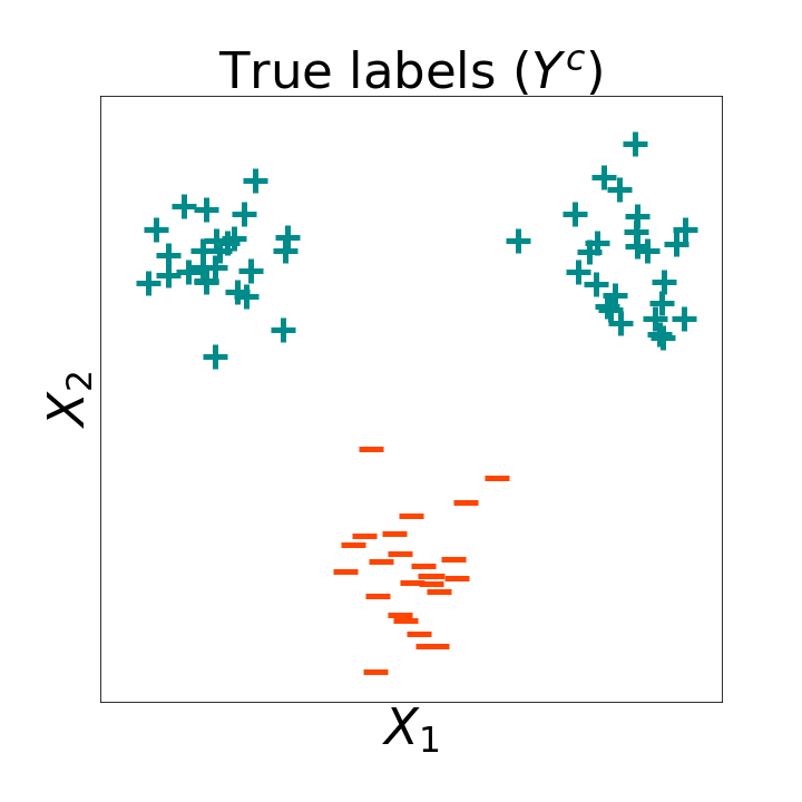
(a)

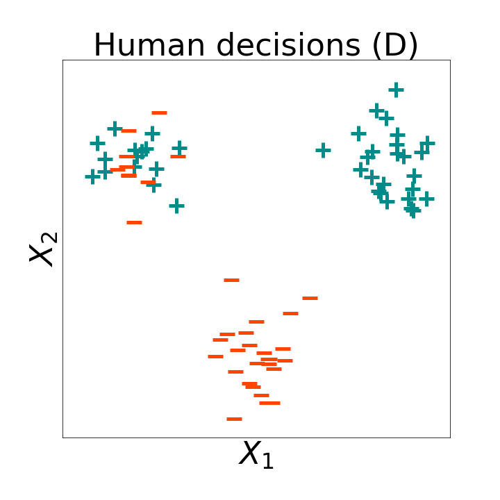
(b)

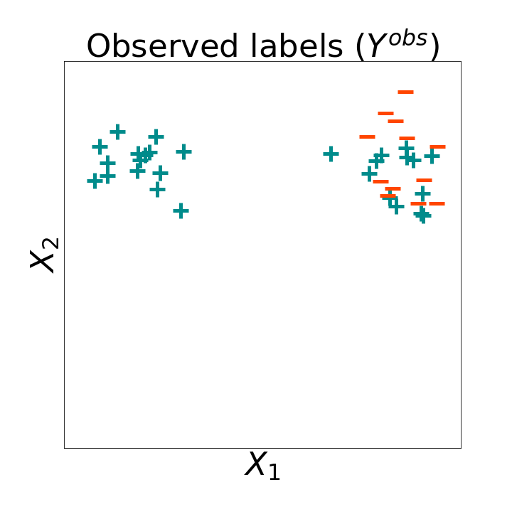
(c)

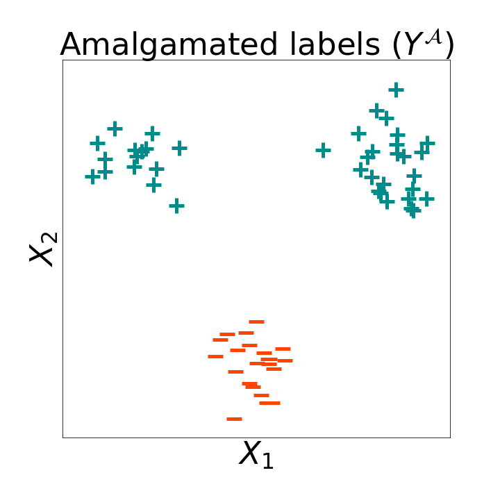
(d)

Figure 3: Toy example illustrating label amalgamation when there is both a construct gap and a selective labels problem. (a) True labels $Y^{c}$. (b) Human expert decisions $D$. (c) Observed outcomes $Y$. (d) Amalgamated labels $Y^{\mathcal{A}}$. Selective labels problem prevents us from seeing the outcome whenever the human expert makes the decision (-), and the construct gap leads to the observed outcome not always corresponding to the true label. Label amalgamation allows us to learn the correct relationship for the true labels.

In relation to previous work that studies learning under the selective labels problem, we note that others have proposed ways to improve validation by leveraging heterogeneity of expert decisions (Kleinberg et al., 2017, Lakkaraju et al., 2017), with a particular focus on the challenges brought about by the presence of unobservables. We complement this work by proposing a way to improve training by leveraging homogeneity.

Finally, note that when the assumptions necessary to apply sampling bias correction techniques are met, the proposed label amalgamation approach can be seamlessly combined with approaches such as inverse weighting to correct for sampling bias while bridging the construct gap. Note that the human decisions themselves do not suffer from sampling bias, so the methodology to infer expert consistency proposed in Section 3 is unaffected by the selective labels problem.

5.2 Learning under unobservables

Experts often have access to certain sources of information that are not available to the algorithm. For example, a physician may integrate patients’ preferences that are verbally communicated to them but not recorded in medical records. Similarly, in the child welfare context, the algorithm does not have access to the information communicated in the call, which is a crucial source of information for call workers. We explicitly note that the proposed approach to estimate expert consistency, introduced in Section 3, can be applied in the presence of unobservables, i.e. it does not depend on an assumption of ignorability. If a decision $D$ partly depends on an unobservable $Z$ for an instance $\bm{x}_{i}\in X$, this means that covariates recorded in $X$ are not sufficient to fully explain the decision for instance $\bm{x}_{i}$ and thus given a small $\delta$, it is the case that $\delta<P(D=1|X=\bm{x}_{i})<1-\delta$. In other words, by virtue of us being able to estimate with high probability the decision $D$ for the subset $\mathcal{A}$, this means that the decision does not depend on unobservables for that subset of cases. As a result, the proposed approaches to leverage inferred expert consistency introduced in Section 4 neither exacerbate nor mitigate the risks of learning under unobservables when compared to $\hat{f}_{Y}$.

5.3 Learning under shared human biases

When learning from expert consistency, a core assumption is that said consistency is indicative of correctness. This is an assumption that cannot be tested, as observational data of human decisions is insufficient to differentiate between correct and erroneous shared beliefs without making further assumptions. In cases where experts consistently make a decision on the basis of something other than expertise, e.g. shared biases or exclusionary policies, the proposed approach would constitute a pathway for teaching those biases to an algorithm. Thus, domain expertise and contextual knowledge is essential when deciding whether the proposed approach is appropriate.

Shared biases that yield deterministic decisions could lead to algorithmic bias under the propose approach. However, the methodology is robust to shared biases that do not yield deterministic decisions. For example, if experts are more likely to make a certain decision for one group than for other, this will not be absorbed by the proposed methodology as long as the decision is not near-deterministic for either group. For example, if the parameter $\delta$ is chosen such that $\delta=0.05$, shared biases may only be learned if there is one subgroup for whom a decision is made 95% of the times. The methodology, by relying on the local influence method, is also robust to biases that yield deterministic decisions by one or a few experts, but not widely shared. Section 6 shows the performance of the method under various scenarios of bias, illustrating both its robustness and its failure modes.

While no diagnostic approach can conclusively determine the presence (or absence) of bias reflected in experts’ consistency, and domain knowledge is crucial to the decision of whether leveraging inferred expert consistency is desirable, demographic parity assessment can be used as a diagnostic approach to determine potential bias. Let $\mathcal{G}$ denote a sensitive group, e.g. a racial minority, and let $\tau$ denote a classification threshold. The demographic parity gap $\textrm{Gap}_{dp}$ for predictive model $\hat{f}~{}:~{}\mathrm{R}^{1\times m}\rightarrow~{}[0,1]$, is given by,

$$\textrm{Gap}_{dp}(\hat{f}(\cdot),\tau,\mathcal{G})=\frac{1}{|\{i\in\mathcal{G}\}|}\sum\limits_{i\in\mathcal{G}}\mathbbm{1}(\hat{f}(\bm{x}_{i})>\tau)-\frac{1}{|\{i\notin\mathcal{G}\}|}\sum\limits_{i\notin\mathcal{G}}\mathbbm{1}(\hat{f}(\bm{x}_{i})>\tau)$$ (28)

Demographic parity is a measure of algorithmic fairness that considers the difference in rates of a given prediction across groups (Chouldechova, 2017). Its main operational advantage lies on the fact that it does not require access to a “ground truth” label. This also constitutes its main disadvantage: differences in rates are not conclusively indicative of disparities in error rates, since base rates may differ across groups.

It can be useful to consider how the demographic parity gap is affected by label amalgamation, let $\tau_{Y}$ and $\tau_{\mathcal{A}}$ denote classification thresholds for $\hat{f}_{Y}$ and $\hat{f}_{\mathcal{A}}$, respectively, which may be different if calibration is different across classifiers and one wants to compare disparities at a fixed selection rate. The shift in demographic parity gap is given by,

$$\Delta\textrm{Gap}_{dp}=\textrm{Gap}_{dp}(\hat{f}_{\mathcal{A}}(\cdot),\tau_{\mathcal{A}},\mathcal{G})-\textrm{Gap}_{dp}(\hat{f}_{Y}(\cdot),\tau_{Y},\mathcal{G})$$ (29)

If the demographic parity gap changes, that is not necessarily indicative of bias. For example, in the context of predicting patients in need for high-cost care management programs, researchers found that the observed outcome that was chosen as a proxy target for a predictive model disadvantaged Black patients (Obermeyer et al., 2019). In such a case, if integrating expert consistency allowed us to better approximated the construct of interest, then the demographic parity gap should change. However, changes that align with societal biases and cannot be explained by domain knowledge may be indicative of a potential risk of bias. For example, in the child welfare domain, we consider whether leveraging inferred expect consistency significantly changes the racial and socioeconomic distribution of screened in cases in a manner that aligns with concerns regarding potential biases in the child welfare system (Eubanks, 2018).

6 Analysis and results

In this section, we first validate the proposed methodology using the publicly available Medical Information Mart for Intensive Care Emergency Department (MIMIC-ED) dataset (Johnson et al., 2021), making use of simulation strategies to assess the method’s performance under different scenarios of human expertise and biases. After providing validation in a controlled setting, we move on to the main empirical findings of our work, which focus on the child welfare context, a high-stakes domain in which algorithmic decision support tools are increasingly being deployed (Chouldechova et al., 2018, Saxena et al., 2020).

6.1 Experimental Setup

In all experiments, we compare performance across five models, including three reference models and two proposed approaches. Given the similarity between empirical performance of the proposed hybrid and deferral models, we choose to only include one of the two to avoid redundancy (see Section 4.2 for detailed discussion). The assessed models are the following:

• $\hat{f}_{Y}$: Model trained to predict an observed outcome, $Y$.

• $\hat{f}_{h}$: Model trained to predict human decisions, $D$.

• $\hat{f}_{Madras}$: Deferral model proposed by Madras et al., (2018).

• $\hat{f}_{\mathcal{A}}$: Proposed model trained on amalgamated labels, as defined in Equation (23).

• $\hat{f}_{hyb}$: Proposed hybrid model, as defined in Equation (27).

We include $\hat{f}_{Madras}$ to show how our method compares to other approaches that leverage and combine human expertise and observed outcomes. Recall that $\hat{f}_{Madras}$ has a different goal from ours, and jointly learns to defer in cases where it assesses that $D$ will have good performance with respect to the observed $Y$, while specializing in the remaining instances.

For all models, we use neural networks with ReLu activation functions. We select the number of hidden layers using cross-validation over the grid $[1,2,3]$, with all layers containing 50 neurons. Models were trained using 1000 epochs with batch size 100, with an Adam optimizer with learning rate 0.001 and a dropout of 0.5. An early stopping criterion was used; if loss increases for 3 iterations on a holdout set defined as 15% of the training split (the holdout portion is not used in training). Additionally, for instances in which we consider a logistic regression alternative (Section 6.3), we note that this can be expressed as a neural network with no hidden layers. When applying the proposed methodology to estimate expert consistency, we ensure the existence of the inverse of the Hessian by adding the smallest L₁ regularization necessary, iteratively exploring values in $[10^{-3},10^{-2},10^{-1},10^{0},10^{1},...]$. To ensure calibration, a Platt scaling was used. We use Monte Carlo cross-validation with 75% train–25% test splits, and report normal confidence bounds at 95% level estimated over 10 iterations. In all splits, we ensure that all experts have representation across all folds, and in the child welfare scenario we adittionally ensure that all cases associated to a same call are in the same fold.

6.2 Decision-making simulations

In the first set of experiments, we study the performance of the model in simulations, and using a publicly available dataset. Consider the tasks of triaging or screening patients for priority care (Caruana et al., 2015, Hong et al., 2018, Raita et al., 2019, Obermeyer et al., 2019). As previously discussed, it has been shown that prioritizing patients for high-cost care management programs using healthcare costs as a proxy for healthcare needs can result in biases due to issues of construct validity (Obermeyer et al., 2019). Similarly, models that aim to support triaging decisions by predicting observed outcomes such as hospitalization or medical complications may fail to identify patients whose needs are not reflected on those outcomes or for whom appropriate prioritization resulted in a positive outcome (Caruana et al., 2015). In this section, we use this motivating example to study the methods’ performance in controlled simulations.

Using the MIMIC-ED dataset (Johnson et al., 2021), we use vital signs measured at admission to the emergency room as covariates $X$, and simulate different scenarios of the potential relationships between observed outcome $Y$, construct of interest $Y^{c}$, and human decisions $D$. In particular, we assume that an algorithmic triaging tool is trained to predict risk of hospitalization (Hong et al., 2018, Raita et al., 2019), but not all patients that require prioritization result in hospitalization. As a proof of concept, we assume that patients who report high levels of pain or who are older than 65 also require prioritization, and humans do take this into consideration (with varying degrees of accuracy and bias). We use tree-based structures to model the relationship between the covariates and the outcomes of interest, and leverage these structures to simulate different settings of human expertise and biases, assuming that there are 20 triage experts who assess cases. Unless otherwise stated, we assume a random experts-to-cases assignment. The full details of the simulation are included in Appendix B.1 and analogous results to all simulations assuming there is a selective labels problem are included in Appendix B.3. In this set of experiments, parameters were fixed to conservative values $(\delta,\gamma_{1},\gamma_{2},\gamma_{3})=(0.05,6,0.95,0.002)$, further sensitivity analyses are performed in Appendix B.2.

6.2.1 Learning from imperfect experts

We first study a set of scenarios that consider different degrees and types of erroneous beliefs. These consider the homogeneity/heterogeneity across experts, i.e. whether they are all equally likely to make a mistake for a given case, and the error frequency. In particular, we explore the following:

• Correct, homogeneous beliefs (CHo): In this setting, decisions are either random or highly accurate. We assume that experts are bad at assessing patients who will be hospitalized but who are younger than 65 year old and who do not present pain, making random decisions in these cases. We also assume that they can predict with very high accuracy the needs of all other patients, even if the patients may not require hospitalization.

• Correct and incorrect, homogeneous beliefs (CIHo): In this setting, incorrect decisions are no longer random. We assume that experts are bad at assessing younger patients who will be hospitalized but who do not present pain—incorrectly screening out 72% of these cases—but they can predict with very high accuracy the needs of all other patients, even if the patients may not require hospitalization.

• Correct and incorrect, heterogeneous beliefs (CIHe): In this setting, we assume that not all experts are equally likely to make a correct decision, and instead they have varying performance when assessing younger patients who will be hospitalized but who do not present pain. For each expert, the probability of error in these cases is $p_{h}$, for $p_{h}\sim\mathcal{U}(a,b)$. We assume they can all predict with very high accuracy the needs of all other patients, even if the patients may not require hospitalization. We consider three variations of this setting:

  • $p_{h}\sim\mathcal{U}(0.3,0.6)$. Some experts have above-random performance when assessing younger patients who will be hospitalized but who do not present pain, and some have worse-than-random performance. Above-random performance is more common.

  • $p_{h}\sim\mathcal{U}(0.5,0.8)$. All experts have worse-than-random performance when assessing younger patients who will be hospitalized but who do not present pain. The worst performing expert still correctly identifies at least 20% of patients among this group who need prioritization.

  • $p_{h}\sim\mathcal{U}(0.7,1.0)$. All experts systematically misdiagnose younger patients who need prioritization when patients do not present pain but will be hospitalized. Some experts may erroneously screen out all patients they assess from this pool.

Table 1 shows results under these different scenarios, reporting area under the receiver operating characteristic (ROC) Curve (AUC) with respect to $Y^{c}$, which is known in the context of simulations. Across all scenarios, label amalgamation yields the best performance, improving significantly when compared to all other alternatives. The benefits of the proposed methodology are especially evident when comparing it with $\hat{f}_{h}$; even in settings where a model trained on expert assessments alone would yield worse than random performance, the proposed methodology is able to extract valuable information contained in experts’ decisions to obtain substantial performance improvements with respect to all alternatives.

Among the two proposed approaches, only label amalgamation consistently outperforms $\hat{f}_{Y}$, indicating that it may be more productive to incorporate inferred consistency at training time. It is worth noting, however, that both approaches perform at least as good as $\hat{f}_{Y}$ across all settings.

Scenarios	$\hat{f}_{Y}$	$\hat{f}_{h}$	$\hat{f}_{Madras}$	$\hat{f}_{\mathcal{A}}$	$\hat{f}_{hyb}$
CH	0.796 (0.004)	0.544 (0.020)	0.767 (0.006)	0.858 (0.008)	0.794 (0.006)
CIHo	0.796 (0.004)	0.432 (0.006)	0.769 (0.003)	0.860 (0.004)	0.798 (0.010)
CIHe (0.7 - 1)	0.796 (0.004)	0.425 (0.003)	0.769 (0.005)	0.860 (0.005)	0.800 (0.008)
CIHe (0.5 - 0.8)	0.796 (0.004)	0.475 (0.018)	0.770 (0.003)	0.858 (0.007)	0.797 (0.005)
CIHe (0.3 - 0.6)	0.796 (0.004)	0.547 (0.011)	0.766 (0.004)	0.860 (0.006)	0.794 (0.005)

Table 1: Methods’ Area under the ROC Curve (AUC) with respect to $Y^{c}$ in different simulations of experts’ decisions, corresponding to different assumptions of human expertise and errors.

6.2.2 Learning from biased experts

We also explore what happens when there are shared human biases that systematically underserve one demographic subgroup. In particular, we assume the presence of a bias that increases the likelihood that women who require prioritization would be erroneously screened out. For the purpose of stress-testing the method, the settings we consider are likely more extreme than what is likely to occur in practice. After considering multiple settings under which the method should in theory be robust, we consider a setting in which the method is bound to fail, in order to provide empirical evidence of the importance of considering whether the method’s assumptions are appropriate when choosing to apply it in practice. The following settings are assessed:

• Deterministic bias, partially shared (DeP): We assume that 50% of experts exhibit a deterministic bias that leads them to screen out all women, regardless of whether they need prioritization.

• Homogeneous bias, fully shared (HoF): We assume that all experts exhibit bias that leads them to screen out 80% of women who should be prioritized.

• Non-random expert-to-patient assignment, near-deterministic bias (nRnD): We assume a non-random assignment under which one expert assesses 95% women, and decides to screen out all of them.

• Deterministic bias, fully shared (method’s assumptions violation) (DeS): Finally, we consider what happens when the method’s assumptions are violated. In this setting, we assume all experts have a deterministic bias that leads them to screen out all women.

Scenarios	$\hat{f}_{Y}$	$\hat{f}_{h}$	$\hat{f}_{Madras}$	$\hat{f}_{\mathcal{A}}$	$\hat{f}_{hyb}$
DeP	0.795 (0.005)	0.669 (0.010)	0.774 (0.006)	0.816 (0.004)	0.790 (0.007)
HoF	0.795 (0.005)	0.612 (0.020)	0.776 (0.003)	0.807 (0.007)	0.790 (0.006)
nRnD	0.795 (0.005)	0.615 (0.008)	0.777 (0.005)	0.801 (0.009)	0.791 (0.007)
DeS (fail mode)	0.795 (0.005)	0.544 (0.003)	0.774 (0.005)	0.602 (0.020)	0.539 (0.004)

Table 2: Methods’ Area under the ROC Curve (AUC) in different simulations of experts’ decisions, corresponding to different assumptions of human’s shared bias.

Scenarios	$\hat{f}_{Y}$	$\hat{f}_{h}$	$\hat{f}_{Madras}$	$\hat{f}_{\mathcal{A}}$	$\hat{f}_{hyb}$
DeP	0.191 (0.004)	0.083 (0.015)	0.181 (0.004)	0.186 (0.004)	0.184 (0.005)
HoF	0.191 (0.004)	0.117 (0.014)	0.184 (0.005)	0.181 (0.004)	0.180 (0.005)
nRnD	0.191 (0.004)	0.122 (0.005)	0.185 (0.004)	0.180 (0.002)	0.178 (0.003)
DeS (fail mode)	0.191 (0.004)	0.078 (0.001)	0.182 (0.007)	0.113 (0.013)	0.078 (0.001)

Table 3: Methods’ True Negative Rate (TNR) for women in different simulations of experts’ decisions, corresponding to different assumptions of human’s shared bias.

Scenarios	$\Delta\textrm{Gap}_{dp}$
DeP	-0.104
HoF	-0.186
nRnD	-0.210
DeS (fail mode)	-0.588

Table 4: $\Delta\textrm{Gap}_{dp}$ as defined in Equation (29), across different simulations of experts’ decisions, corresponding to different assumptions of human’s shared bias.

Table 2 shows results under these different scenarios, reporting AUC with respect to $Y^{c}$. Across all settings in which the method is expected to be robust, label amalgamation yields modest improvements or comparable performance to $\hat{f}_{Y}$. The proposed method should prevent errors, idiosyncrasies and biases (other than those that violate the method’s core assumption) from being absorbed by the model. Given that the bias considered in these simulations results in disproportionate false negative errors for women, its robustness to bias can be better studied through the true negative rate (TNR) for this demographic subgroup, which is reported in Table 3. The classification threshold is set to a 30% screen out rate, which corresponds to the screen-out rate in the real-world data. Across all settings (except failure mode), the TNR of the proposed approaches is comparable to that of $\hat{f}_{Y}$, even when $\hat{f}_{h}$ exhibits substantially worse TNR. Appendix B.2 further explores the nRnD scenario to explore how parameters might impact performance in a biased setting.

Importantly, if the assumptions are violated and expert consistency is a result of bias that yields near-deterministic decisions and is shared by all experts, the proposed approach is detrimental to overall performance, as shown in Table 2. Moreover, the TNR for women, shown in Table 3, allows us to observe that in this setting the proposed approach absorbs the bias of the experts with respect to the disadvantaged subgroup. This result highlights the importance of integrating domain knowledge when deciding whether the proposed approach is suitable.

Given that we have access to an oracle in these simulations, one of the most reliable ways of assessing bias is through error rates. However, because this assessment is not possible in real-world settings, we also consider the demographic parity assessment $\Delta\textrm{Gap}_{dp}$ defined in Equation (29). This statistic, reported in Table 4, shows the change in selection rates across genders when using amalgamation vs. relying on observed outcomes alone. These results illustrate two things that were discussed conceptually in Section 5.3. First, we see that a non-zero value is not necessarily indicative of increased error rates for one group, emphasizing the fact that demographic parity disparities suggest a potential issue and should not be treated as conclusive evidence. Second, the very large value seen in the failure mode indicates that this diagnostic can serve as a red light suggesting the risk of inferred consistency carrying bias. As such, an interpretation of this diagnostic grounded on domain knowledge can support the decision of whether it may be desirable to integrate inferred expert consistency in a given setting.

6.3 Child maltreatment hotline screening decisions

Having studied the effectiveness of the approach in simulation settings, we now turn to real data from a high-stakes domain in which algorithmic decision support tools are increasingly been deployed.

6.3.1 Context

In the United States, over 4 million calls concerning potential child neglect or abuse are received by child maltreatment hotlines every year (U.S. Department of Health and Human Services, 2020). Call workers who receive these calls are tasked with deciding which cases should be screened-in for further investigation. Due to the high volume of calls, not all calls can be investigated, and the county recognizes the burden placed on a family when an investigation concerning potential child neglect or abuse is opened. These reasons constitute an incentive to screen out cases where there is no risk to the child (reduce false positives). However, failing to identify risk can lead to a fatal outcome for a child, which highlights the insurmountable cost of false negatives. This context, and the fact that the information communicated in a call can often be insufficient to establish if a child is at risk, has led many jurisdictions to grant call workers access to different databases, including criminal history and utilization of state public assistance programs. Efforts to increase the availability of historical information about children and adults involved in a call have been accompanied by an interest in the use of ML models for risk prediction (Chouldechova et al., 2018).

Allegheny County, PA, USA, where child maltreatment hotlines record 15,000 calls each year, has already implemented one such system. A predictive model is trained to estimate the probability that an investigation will result in an out-of-home placement of the child using multi-system administrative data as covariates. Prior to the deployment of the model, call workers had access to the information communicated in the referral call, as well as direct access to the multi-system administrative data, including demographics, child welfare involvement, criminal history, and other information related to the children and adults associated to a referral. Since the deployment of the predictive model, this information is complemented with the model’s predictions. Important for the purpose of this paper, the assignment of calls to call workers is non-random, as it depends on the shift of the workers (different types of calls are received on different days of the week and at different times of the day).

Work considering the impacts of predictive algorithms in the child welfare context have considered the risk of further marginalizing historically underserved communities (Eubanks, 2018), the perceptions and concerns of the affected communities (Brown et al., 2019), and the importance of call workers’ discretionary power in the face of algorithmic errors (De-Arteaga et al., 2020). For a review of the literature, we refer the reader to Saxena et al., (2020).

6.3.2 Construct gap

We focus our attention on the construct gap between the algorithm’s objective and the decision objective. The algorithm is trained to predict the probability of out-of-home placement, $Y$. However, the call workers’ goal is to screen in cases where the child may be at risk. Fortunately, not all cases where there is a risk to the child require that the child be placed out of the home, and a number of other interventions and forms of support are available to reduce the risk to the child without requiring a family separation. The county has chosen to prioritize this outcome due to its severity, both because it may help prioritize cases most at risk and because the gravity of an out-of-home placement means that this outcome is less subject to noise and to individuals’ idiosyncrasies.

Recent work, however, has shown that deploying decision support tools that optimize for narrowly circumscribed outcomes may shift the criteria people use for making decisions (Green and Chen, 2021). In the child welfare context, this could pose a serious risk. Choosing to screen in calls based on the likelihood of out-of-home placement could result in an agency that primarily intervenes when a case will result on a family separations. This could in turn increase the risk to children for whom early interventions and other forms of support yield positive outcomes.

The availability of other outcomes of interest that are recorded in the data but never observed by the model, either as covariates or as target labels, provides a unique opportunity to evaluate the proposed approach. The first of these outcomes is “substantiation”, which encodes whether the social worker who visits the home deems the claims communicated in the call to be substantiated. The second outcome is “services”, which records if services are offered to the family as a result of the investigation. These outcomes shed light on other important dimensions that are highly relevant to the construct that the agency cares about: risk to the child.

In our experiments, we study whether improving performance with a narrow focus on out-of-home placement may come at a cost to performance on other dimensions relevant to the decision goal. It is important to empirically study this because an imperfect construct does not necessarily imply that the performance compared to the status quo will drop for cases whose risk is not wholly captured in the observed label. If there is enough colinearity across outcomes, and depending on experts’ performance, an imperfect proxy could still provide improvements along dimensions of the decision goal that are not directly observed by the algorithm. Importantly, while in this specific domain we have access to complementary observed outcomes that enable validation, this is a rare circumstance, which is why we focus on methodologies that may bridge the construct gap without observing these outcomes, and only use them for evaluation purposes.

6.3.3 Data

The data used in our experiments corresponds to $46,544$ referrals (i.e. calls) received by Allegheny County between 2010 and 2014. This subset includes the first call associated to each child in this period of time, during which no risk assessment model was deployed. Over 800 variables are available, including information regarding demographics, behavioral health, and past interactions with county prison and public welfare for all adults and children associated to a referral. A detailed explanation of the Allegheny County Department of Human Services Data Warehouse and its use for predictive modeling can be found on the county’s website (Allegheny County Department of Human Services, 2020).

The observed label, $Y$, records whether out-of-home placement is observed in the 730 days following a call. In addition to this outcome, there are other outcomes of interest that are recorded but never observed by the model, either as covariates or as target labels. $Y_{sub}$ records if the social worker who visits the home deems the claims communicated in the call to be substantiated, and $Y_{serv}$ records if services are offered to the family as a result of the investigation. All these outcomes may only be observed if the call is screened in for investigation, meaning that there is a selective labels problem.

6.3.4 Predictive models and evaluation

We follow the experimental setup described in Section 6.1 with $(\delta,\gamma_{1},\gamma_{2},\gamma_{3})=(0.05,4,0.8,0.002)$ (see sensitivity analysis and rationale for parameters’ choice in Appendix C.2). We evaluate both neural networks and logistic regression. This ensures that we consider both a state-of-the-art model and a model that is frequently used in these settings. In this domain, like in other high-stakes settings that use administrative data, less complex models often exhibit comparable performance and are favored for deployment, given their relative interpretability and lower computational expense.

Unlike the simulations in Section 6.2, where we could assume access to an oracle, in this context the selective labels problem prevents the outcomes from being observed for all cases. This deems AUC an inappropriate approach to evaluate performance. Instead, we evaluate precision curves, showing precision when the classification threshold varies to include the top p% highest scored screened-in cases. While not able to provide an oracle evaluation, these metrics provide a path to assess the different models by comparing them on the basis of their relative prioritization of cases for which we observe an outcome.

6.3.5 Results

Figure 4 shows precision curves of all models with respect to the outcome $Y$ (out-of-home placement) and additional outcomes that are not observed by the models (services and substantiation). Some cut-offs have more practical relevance than others. While the decision support tool does not provide binary recommendations, the screen-in rates have remained constant throughout the years, even after the deployment of the tool (De-Arteaga et al., 2020). The county has resources to screen in approximately 40% of the calls, and many calls are screened in solely on the basis of the information communicated in the call, therefore it is reasonable to assume that cutoffs around 25%-35% have the most practical relevance. Figure 5 shows precision at a 25% cut-off.

Figure 4: Precision on child maltreatment risk assessment for top $p\%$ highest scored screened-in cases by model, using neural networks for all models. Error bars show mean$\pm$95%-CI over 10 runs of $75-25\%$ Monte Carlo cross-validation. ‘Overall prev.’ corresponds to the percentage of the evaluation population observing a given outcome. Results show that (1) there are elements of risk that are not captured by the model trained to predict out-of-home placement label $\hat{f}_{Y}$, but are optimized for by humans, and (2) label amalgamation improves precision for these cases, while having a better performance on out-of-home-placement than a model trained on human decisions alone.

Figure 5: Precision on child maltreatment risk assessment for top $25\%$ highest scored screened-in cases by model.

Consistent with what we observe in simulations, the results show that among the approaches that we propose, amalgamation yields better results than the hybrid model. When comparing $\hat{f}_{Y}$ and $\hat{f}_{h}$, we observe that a model trained on human decisions has substantially higher performance for cases that require services and for those that are substantiated, while $\hat{f}_{Y}$ fails to prioritize these cases. This suggests that there are cases whose risk is considered by experts but not captured in the target labels used to train a deployed model.

However, there is a big gap in the other direction when assessing models with respect to out-of-home placement, where the performance of $\hat{f}_{h}$ lags significantly behind. Meanwhile, $\hat{f}_{\mathcal{A}}$ successfully incorporates expert knowledge, considerably improving precision for cases that are substantiated and to which services are offered, while retaining performance with respect to out-of-home placement.

Assessing a previously proposed model to learn to defer, $\hat{f}_{Madras}$, shows that its performance is comparable to $\hat{f}_{\mathcal{A}}$ for out-of-home placement prediction, but is significantly worse for substantiation and services. This is not a surprise given that this method aims to improve performance with respect to $Y$ and does not consider the construct gap, but the results provide empirical evidence showing that different criteria for combining observed outcomes and expert assessments can achieve significantly different goals.

In some domains, including child welfare, less complex models are favoured for deployment, and thus relying on complex models such as neural networks can hamper the likelihood that a model will be adopted in practice. Furthermore, when relying on structured data such as administrative data, simpler models can often achieve comparable performance. This is the case for the proposed methodology in this domain. Figure 6 shows precision curves when all models rely on logistic regression. Figure 10 in Appendix shows precision at a 25% cut-off. While the complexity of neural networks is of importance for $\hat{f}_{Madras}$, all other models exhibit comparable performance to what was observed with neural networks. This highlights the feasibility of applying the proposed methodology in contexts that favor limited model complexity.

Figure 6: Precision on child maltreatment risk assessment for top $p\%$ highest scored screened-in cases by model. All models are logistic regression. Error bars show mean$\pm$std over 10 runs of $75-25\%$ Monte Carlo cross-validation. Results show that (1) there are elements of risk that are not captured by the model trained to predict out-of-home placement label $\hat{f}_{Y}$, but are optimized for by humans, and (2) label amalgamation improves recall and precision for these cases, while having a better performance on out-of-home-placement than a model trained on human decisions alone.

One concern of integrating inferred expert consistency in this setting would be if widespread stereotypes held by call workers are incorporated into the model. In particular, it would be worrying if racial disparities arise (Eubanks, 2018). Table 5 shows the racial breakdown when using a 25% cut-off. Appendix C.1 shows the analogous result when using logistic regression. This provides preliminary indication that label amalgamation in this setting would not exacerbate nor mitigate racial biases.

In light of recent work showing that relying on automated prediction tools could exacerbate disparities when compared to humans and to human-AI collaboration systems (Cheng et al., 2022, Fogliato et al., 2022), we note that those results also show that humans-in-the-loop mitigate bias with respect to the algorithm (which in this case would be $\hat{f}_{Y}$) because they integrate unobserved covariates (Fogliato et al., 2022), and thus neither $\hat{f}_{h}$ nor the proposed methodology can leverage this positive property of expert assessments. In this regard, it is important to emphasize that the proposed method should only be considered as a decision support tool and not as an autonomous system. Finally, it is also worth noting that racial diparities in screen-in rates are only one of many ethical concerns that may arise, some of which cannot be evaluated through statistical tests alone and instead require a careful analysis of the sociotechnical context in which the system is embedded. As such, this evaluation does not constitute a recommendation that the proposed approach should be deployed in the child welfare context, which is a decision that would require a more holistic assessment.

	% Black screen-in
Model	Entire population	Screened-in population
$\hat{f}_{D}$	$51.93(0.69)$	$51.02(0.63)$
$\hat{f}_{Y}$	$48.79(0.91)$	$52.39(1.09)$
$\hat{f}_{Madras}$	$49.49(2.46)$	$53.83(2.41)$
$\hat{f}_{\mathcal{A}}$	$50.00(0.72)$	$50.88(0.66)$
$\hat{f}_{hyb}$	$49.58(1.18)$	$52.10(1.55)$
Overall population	$40.49(0.43)$	$46.10(0.53)$

Table 5: Percentage (95%-CI) of calls that involve at least one Black children when considering top 25% highest-scoring screened-in cases with the neural network approach. Results are shown when considering the top 25% highest scored cases overall, and the top 25% highest scored screened-in cases. This result provides preliminary indication that the proposed label amalgamation does not introduce racial biases.

7 Discussion

This paper tackles the gap between decision objectives and algorithm objectives by leveraging historical expert decisions stored in organizational information systems. While observed outcomes alone often provide a myopic view of the actual construct of interest, expert decisions hold valuable information that can help us bridge the construct gap. However, extracting information contained in historical expert decisions is not straightforward, as experts may be mistaken, noisy or biased. In particular, current expert knowledge may often be sufficient to correctly and consistently assess subsets of cases, while being insufficient for assessing others. It is therefore desirable, yet non-trivial, to learn from experts for subsets of cases for which they consistently make the same decision. In this work, we propose a methodology to estimate consistency across experts on the basis of their historical decisions that involve a single decision per case. The proposed approach uses influence functions to enable consistency estimation when there is a non-random assignment of experts-to-cases, a common circumstance across application domains. Using the inferred expert consistency as a cornerstone, we then propose a label amalgamation approach to learn from experts in cases where experts exhibit consistency, and learn from observed outcomes elsewhere. We complement this proposed amalgamation with alternatives that make use of inferred consistency at prediction time, via deferral or hybrid models.

Results on simulations show that the proposed methodology is successful across various scenarios of expert decision-making, including multiple variations in which humans share biases. In the context of child maltreatment hotline screenings, a domain in which risk assessment tools have been deployed to help call workers identify cases that should be screened in for investigation, our results indicate that there are elements of risk that are not wholly captured in the target label optimized for in deployed models, but which are optimized for by hotline call workers. This provides empirical evidence for the need to bridge the construct gap in this domain, since narrowly optimizing for out-of-home placement could risk failure in supporting children and families who would benefit from services and other interventions available to them. The proposed approach yields a model that improves precision for these cases, while retaining predictive power with respect to out-of-home-placement.

Limitations.

The underlying assumption of the proposed approach is that experts’ consistency is a valuable source of information. This is a reasonable assumption in many applications, where experts’ decisions are grounded in deep domain knowledge and scientific discoveries. However, learning from expert consistency may not always be desirable. Two prominent risks include the possibility of experts’ decisions reflecting shared societal biases and self-fulfilling prophecies. While the results in Section 6.2 show that the approach is robust to many forms of shared biases, they also provide empirical illustration of what may happen if near-deterministic decisions are a result of bias shared among experts. In addition to shared societal biases, erroneously held beliefs may stem from self-fulfilling prophecies. In the clinical domain, for instance, this corresponds to cases in which a physicians’ belief of a patients’ poor prognosis leads them to withdraw treatment, hence making the initial prediction more likely to come true (Wilkinson, 2009). Because self-fulfilling prophecies can inform future practices, these can be reflected in experts’ consistency. Importantly, however, self-fulfilling prophecies also affect observed outcomes, hence the proposed approach would neither exacerbate nor ameliorate this problem.

Other uses of labelers’ influence estimation.

A fundamental contribution of this work is the use of the local influence method to estimate individual labelers’ influence over predictions. We have used this approach to estimate consistency, and we have proposed ways of leveraging the inferred consistency to overcome limitations of algorithmic decision support tools. We expect there to be many more applications of our proposed labelers’ influence estimation approach. For instance, we anticipate that there could be promising applications to improve crowdsourcing, especially in contexts in which not all labelers are equally well positioned to assess different instances (Davani et al., 2022, Fazelpour and De-Arteaga, 2022). Drawing connections to the use of influence functions to improve robustness to adversarial attacks (Koh and Liang, 2017), it could also be valuable in analyzing whether and how a low performing or adversarial expert or labeler could affect predictions of models trained on human decisions.

Other approaches to estimate and leverage experts’ consistency.

Throughout our work, we have made many methodological choices in choosing how to estimate consistency, as well as how to leverage it. We anticipate that there could be multiple alternative avenues to tackle the same problems. We have given various alternatives for how to leverage expert consistency, but we do not expect these to be the only possibilities. For example, one could explore the integration of inferred consistency and observed outcomes as a means to tackle other challenges in human-AI collaboration, such as estimating and communicating uncertainty (Bhatt et al., 2021). Additionally, one could potentially develop other approaches to infer expert consistency through means other than influence functions. If there are enough instances per expert to train a classifier based on each of them, one could explore boosting approaches to productively integrate these. Similarly, Bayesian approaches are a natural fit to integrate different sources of labels, and could potentially be used both to estimate and leverage consistency.

Other implications for trust and deployment.

Throughout this paper, we have discussed how the proposed approach can help mitigate the construct gap, and we have also discussed its value in the context of selective labels, especially when expert consistency results in a positivity assumption violation. However, there may be other implications and motivations for incorporating inferred expert consistency into algorithmic decision support tools. First, different types of labels and informational sources may encode different biases, and thus jointly learning from them may reduce bias overall. Empirically and theoretically studying this is a valuable direction for future work. Additionally, there may be implications for trust that may affect the human-algorithm relationship and the experts’ willingness to adhere to the algorithmic recommendations. Previous work has discussed the phenomenon of algorithm aversion, and the fact that humans easily loose trust on algorithmic tools after seeing them err (Dietvorst et al., 2015). Not all errors may have the same implications on trust, and there is a risk that algorithmic errors and disagreement in cases where experts are very confident in their own assessment can be more detrimental to the experts’ trust in the algorithm.

Incorporating experts’ knowledge into algorithmic decision support tools may also have important implications when the experts whose knowledge is encoded into the algorithm are not the same as those using the algorithm. In particular, when algorithmic decision support tools are developed at highly specialized institutions and deployed widely, incorporating expert knowledge into the model may be of special relevance and may serve as a pathway to transfer knowledge from top experts to other facilities and organizations. For instance, when developing a decision support tool for healthcare, clinicians at research institutions may have expertise allowing them to easily assess some cases. If an algorithmic tool is trained on observed outcomes alone, it is possible that those clinicians could easily dismiss erroneous algorithmic recommendations when they conflict with their own assessments. However, the same may not be true for other clinicians that may lack such expertise, and whose decisions could benefit from the expertise harvested from lead institutions and encoded into decision support algorithms.

Appendix A Challenges of algorithmic decision support and modeling human decisions

The relationship between $\hat{f}_{h}$ and $\hat{f}_{Y}$ is informative of the potential benefits and risks of using $\hat{f}_{Y}(x)$ as a decision support tool. Figure 7 and Table A present an overview of possible sources of disagreement between these models. Here, we describe the relationship based on the regions shown in Figure 7. For the purpose of this explanation, assume the outcome $Y$ is observed when $D=1$, meaning $\hat{f}_{Y}=\hat{P}(Y|X,D=1)$.

Figure 7: Diagram of possible relationships of $\hat{f}_{h}(\bm{x})$ and $\hat{f}_{Y}(\bm{x})$.

Table 6: Possible biases that may yield relationships between $\hat{f}_{h}(x)$ and $\hat{f}_{Y}(x)$ in given regions of the plot. Questions indicate that this is only a possibility, with the alternative being that humans are not making the correct decisions. Each column corresponds to a selective labels setting.

Region	$\hat{f}_{Y}=\hat{P}(Y|X,D=1)$	$\hat{f}_{y}=\hat{P}(Y|X,D=0)$
A	Agreement region.
B	Positivity assumption violation under selective labels problem.	Construct gap?
C	Unobservables?	Unobservables and construct gap?
D	Construct gap?	Construct gap?
E	Unobservables and omitted payoff bias?	Unobservables?

Region A.

Subsets of cases that lie on the diagonal of Figure 7, denoted as Region A, are those for which $\hat{f}_{h}(\bm{x})\approx\hat{f}_{Y}(\bm{x})$. For these, the observed outcomes validate the human decisions, but learning a model on observed outcomes does not provide any more information than “automating” the human decisions.

Meanwhile, subsets for which $\hat{f}_{h}(\bm{x})\neq\hat{f}_{Y}(\bm{x})$ may indicate that (1) the humans are making poor decisions or (2) that they are making good decisions but unobservables, selective labels, or omitted payoff biases are at play, leading the model trained on observed outcomes to make incorrect predictions. Importantly, without further information, there is no way of differentiating between these cases on the basis of observational data alone. However, the relationship between $\hat{f}_{h}$ and $\hat{f}_{Y}$ does provide information as to which risks may be present or which assumptions would be required in order to trust one model or the other.

Region B.

Whenever $\hat{f}_{h}$ predicts $D=0$ with high probability for a subset of cases, there is a violation of the positivity assumption. As a result, no labels are observed for this area. Thus, predictions made by $\hat{f}_{Y}$ in this area will constitute an extrapolation.

Region C.

A subset may lie in Region C as a result of humans’ poor decision making or due to unobservables. Here, $\hat{f}_{h}$ displays uncertainty while $\hat{f}_{Y}$ yields high-certainty predictions. If humans are making correct decisions based on an unobserved feature $z$, $\hat{f}_{h}$ will not have enough information to accurately predict $D$, which will be reflected in uncertain predictions, while $\hat{f}_{Y}$ will me making predictions conditioned on the value of $z$. This scenario has been discussed extensively in Kleinberg et al., (2017).

Region D.

Meanwhile, it may be the case that $\hat{f}_{h}$ predicts $D=1$ with high probability, but the model $\hat{f}_{Y}$ learned from observed outcomes provides a contrary assessment. This may be a consequence of humans’ making incorrect decisions—for example, humans may systematically overestimate the risk of a subpopulation. However, this may also be a result of a construct gap.

Region E.

Finally, a rather convoluted setting arises in Region E: either humans are mistaken at least in some cases, or there are both unobserved covariates and a construct gap. Here, the human decisions could only be correct if the presence of unobservables leads $\hat{f}_{Y}$ and $\hat{f}_{h}$ to group together cases that in reality are distinct, and additionally a construct gap leads to the observed outcome not corresponding to the human prediction.

Appendix B Simulation experiments

B.1 Simulations of different scenarios

This section describes the simulations presented in Section 6. Using the MIMIC-ED data, we use vital signs measured at admission to the emergency room as covariates $X$. We define $Y_{1}$ as the observed admission to hospital, and $Y_{2}$ as a binary variable indicating if the patient is over 65 years old or if they report a high level of pain. The covariates seen by the algorithm do not include either of these variables (except when explicitly noted in the simulation for a given scenario).

To ensure that we have full control over the relationship between the covariates and outcomes, and to model different scenarios of human knowledge, errors, and biases, we simulate labels $\tilde{Y}_{1}$, $\tilde{Y}_{2}$ and $D$, as well as the assignment $a$, as described below. We assume $Y^{c}=\tilde{Y}_{1}\bigcup\tilde{Y}_{2}$, and the algorithm only optimizes for $\tilde{Y}_{1}$.

Data: Vital signs measured at triage $X$

Result: Simulation of labels $\tilde{Y}_{1}$ and $\tilde{Y}_{2},$ human prioritization $D$, expert assignment $a$

3 $\tilde{Y}_{1}\leftarrow$ Tree($Y_{1}\sim X$, depth = 15);

4 $\tilde{Y}_{2}\leftarrow$ Tree($Y_{2}\sim X$, depth = 15);

5 $D\leftarrow$ Tree($\tilde{Y}_{1}\cup\tilde{Y}_{2}\sim X$, depth = 10);

6 $a\leftarrow$ Random draw in $[\![1,k]\!]$;

7

8$\mathcal{L}\leftarrow$ Individuals in leaves with 70% prevalence of $\tilde{Y}_{1}$ and intersection $\tilde{Y}_{1}\cap\tilde{Y}_{2}$ inferior to 30%;

9

10for $i\in\mathcal{L}$ do

11       $D_{i}\leftarrow\mathcal{B}ernoulli(0.5)$; Random draw of the human decision for instances in $\mathcal{L}$;

12      

13 end for

Experts are bad at assessing patients who will be hospitalized but who are young and do not present pain, making random decision in these cases.

Data generation - Scenario 1 Correct, homogeneous beliefs

Experts are bad at assessing patients who will be hospitalized but who are young and do not present pain, making random decision in these cases.

Data: Vital signs measured at triage $X$

Result: Simulation of labels $\tilde{Y}_{1}$ and $\tilde{Y}_{2},$ human prioritization $D$, expert assignment $a$

3 Obtain $\tilde{Y}_{1}$, $\tilde{Y}_{2}$, $D$, $\mathcal{L}$, $a$ by executing lines 1 to 5 from Scenario 1;

4 $\mathcal{N}\leftarrow$ Randomly draw $75\%$ of instances in $\mathcal{L}$;

5 for $i\in\mathcal{N}$ do

6       $D_{i}\leftarrow\neg\tilde{Y}_{1,i}$;

7      

8 end for

Experts are bad at assessing patients who will be hospitalized but who are young and do not present pain, making the wrong decision in 75% of the cases.

Data generation - Scenario 2 Correct and incorrect, homogeneous beliefs

Experts are bad at assessing patients who will be hospitalized but who are young and do not present pain, making the wrong decision in 75% of the cases.

Data: Vital signs measured at triage $X$ and base error rate $E$

Result: Simulation of labels $\tilde{Y}_{1}$ and $\tilde{Y}_{2},$ human prioritization $D$, expert assignment $a$

3 Obtain $\tilde{Y}_{1}$, $\tilde{Y}_{2}$, $D$, $\mathcal{L}$, $a$ by executing lines 1 to 5 from Scenario 1;

4 Draw homogeneous error rate for each expert $e_{h}\sim\mathcal{U}([E,E+0.3])$;

5

6for $h\in[\![1,k]\!]$ do

7       $\mathcal{N}\leftarrow$ Randomly draw $e_{h}$ of instances in $\mathcal{L}$ assigned to $h$, i.e. $\{i\in\mathcal{L},a_{i}=h\}$;

8       for $i\in\mathcal{N}$ do

9             $D_{i}\leftarrow\neg\tilde{Y}_{1,i}$;

10            

11       end for

12      

13 end for

Experts have different level of errors for patients who will be hospitalized but do not present pain.

Data generation - Scenario 3 Correct and incorrect, heterogeneous beliefs

Experts have different level of errors for patients who will be hospitalized but do not present pain.

For the biased scenarios introduced in Section 6.2.2, the decision depends on the group membership $M$ with $M_{i}=1$ corresponding to patient $i$ being part of the minority group. In this context, the previously described models have for inputs $X$ and $M$ to allow the models to capture potential relation between group and outcome.

Data: Vital signs measured at triage $X$, Minority membership $M$

Result: Simulation of labels $\tilde{Y}_{1}$ and $\tilde{Y}_{2},$ human prioritization $D$, expert assignment $a$

3 Obtain $\tilde{Y}_{1}$, $\tilde{Y}_{2}$, $a$ and $D$ by executing lines 1 to 4 from Scenario 1;

4 $\mathcal{N}\leftarrow\{i,a_{i}<\frac{k}{2}\land M_{i}=1\}$;

5 for $i\in\mathcal{N}$ do

6       $D_{i}\leftarrow 0$;

7      

8 end for

50% of experts exhibit a deterministic bias that leads them to screen out all women.

Data generation - Scenario 4 Deterministic bias, partially shared

50% of experts exhibit a deterministic bias that leads them to screen out all women.

Data: Vital signs measured at triage $X$, Minority membership $M$

Result: Simulation of labels $\tilde{Y}_{1}$ and $\tilde{Y}_{2},$ human prioritization $D$, expert assignment $a$

3 Obtain $\tilde{Y}_{1}$, $\tilde{Y}_{2}$, $a$ and $D$ by executing lines 1 to 4 from Scenario 1;

4 $\mathcal{N}\leftarrow$ Draw $80\%$ of instances in protected group $\{i,M_{i}=1\}$;

5 for $i\in\mathcal{N}$ do

6       $D_{i}\leftarrow 0$;

7      

8 end for

All experts exhibit bias that leads them to screen out 80% of women.

Data generation - Scenario 5 Homogeneous bias, fully shared

All experts exhibit bias that leads them to screen out 80% of women.

Data: Vital signs measured at triage $X$, Minority membership $M$

Result: Simulation of labels $\tilde{Y}_{1}$ and $\tilde{Y}_{2},$ human prioritization $D$, expert assignment $a$

3 Obtain $\tilde{Y}_{1}$, $\tilde{Y}_{2}$, $a$ and $D$ by executing lines 1 to 4 from Scenario 1;

4 $\mathcal{N}\leftarrow$ Draw $95\%$ of instances in protected group $\{i,M_{i}=1\}$;

5 for $i\in\mathcal{N}$ do

6       $a_{i}\leftarrow 0$; Assign to expert $0$;

7       $D_{i}\leftarrow 0$;

8      

9 end for

10

Non-random assignment under which one expert assesses 95% women, and decides to screen out all of them.

Data generation - Scenario 6 Non-random expert-to-patient assignment, near-deterministic bias

Non-random assignment under which one expert assesses 95% women, and decides to screen out all of them.

Data: Vital signs measured at triage $X$, Minority membership $M$

Result: Simulation of labels $\tilde{Y}_{1}$ and $\tilde{Y}_{2},$ human prioritization $D$, expert assignment $a$

3 Obtain $\tilde{Y}_{1}$, $\tilde{Y}_{2}$, $a$ and $D$ by executing lines 1 to 4 from Scenario 1;

4 for $i\in\{i,M_{i}=1\}$ do

5       $D_{i}\leftarrow 0$;

6      

7 end for

All experts have a deterministic bias that leads them to screen out all women.

Data generation - Scenario 7 Deterministic bias, fully shared

All experts have a deterministic bias that leads them to screen out all women.

B.2 Further analysis of nRnD

Among simulation scenarios, the local influence method is most important for the non-random expert-to-patient assignment, near-deterministic bias scenario (nRnD). This is because in this setting high-probability predictions of human decisions may be driven by a single expert. Figure 8 shows the mean influence per expert, estimated across all cases in each subgroup. Expert 0 is the expert that assesses 95% of women’s cases and always screens them out. In this instance, the local influence method shows that one expert is at odds with the rest, and the prediction of low probability of screen-in is driven by a single expert.

We investigate how this bias impacts the proposed metrics of consensus. Figure 9 shows the agreement metrics differentiated by group. While the center of mass shows that the agreeing proportion of experts is smaller for female than for male patients, the aligned influence identifies a set of patients for which only a small fraction of expert goes in the opposite direction than the majority. This led us to study the impact of varying $\gamma_{2}$. Table 7 shows the performance of the method when varying this parameter. In particular, it can be seen that a threshold including predictions led by one expert integrate the bias against the minority group. However, the model presents robust performance on a large range of the parameter.

Thus, the proposed approach enables a robust estimation of the set $\mathcal{A}$, which would not include high probability predictions driven by a single expert.

Figure 8: Mean influence per expert in setting nRnD, estimated across all cases in each subgroup. Expert 0 is the expert that assesses 95% of women’s cases and always screens them out.

(a) Center of mass

(b) Aligned influence

Figure 9: Measure of consensus in nRnD scenario differentiated by group membership.

$\gamma_{2}$	0.1	0.2	0.35	0.65	0.8
AUC	0.596 (0.010)	0.799 (0.006)	0.799 (0.006)	0.800 (0.005)	0.799 (0.006)
TNRw	0.117 (0.005)	0.179 (0.004)	0.179 (0.004)	0.180 (0.003)	0.179 (0.002)

Table 7: Methods’ Area Under the ROC Curve (AUC) and True Negative Rate for women (TNR_w) computed across different $\gamma_{2}$.

B.3 Performance under selective labels problem

Below we present analogous experiments to all simulations presented in Section 6.2, assuming the presence of the selective labels problem. Here, we assume that outcome $Y$ is only observed when a human decides to screen-in a case, as is the case in the real-world example of child maltreatment hotline screenings. We assume that the selective labels problem affects the labels available for training, but still provide evaluation with respect to an oracle, which assesses performance with respect to $Y^{c}$ for all instances in the test set. Results are presented in Tables 8, 9 and 10. First, note that $\hat{f}_{h}$ is unchanged as the human decision is fully observed. However, all other methods present a drop in performance. This decrease is particularly pronounced for $\hat{f}_{Madras}$. The results show the same patterns observed in the absence of the selective labels problem, and the proposed label amalgamation approach yields the best performance for all cases, except its failure mode.

Scenarios	$\hat{f}_{Y}$	$\hat{f}_{h}$	$\hat{f}_{Madras}$	$\hat{f}_{\mathcal{A}}$	$\hat{f}_{hyb}$
CH	0.782 (0.004)	0.544 (0.020)	0.584 (0.004)	0.846 (0.013)	0.783 (0.004)
CIHo	0.780 (0.004)	0.432 (0.006)	0.489 (0.009)	0.843 (0.007)	0.772 (0.005)
CIHe (0.7 - 1)	0.781 (0.003)	0.425 (0.003)	0.469 (0.029)	0.832 (0.012)	0.770 (0.006)
CIHe (0.5 - 0.8)	0.780 (0.003)	0.475 (0.018)	0.532 (0.015)	0.841 (0.012)	0.776 (0.006)
CIHe (0.3 - 0.6)	0.778 (0.003)	0.547 (0.011)	0.604 (0.004)	0.848 (0.012)	0.781 (0.004)

Table 8: Methods’ Area under the ROC Curve (AUC) with respect to $Y^{c}$ in different simulations of experts’ decisions, corresponding to different assumptions of human expertise and errors. We assume the selective labels problem constrains labels available for training.

Scenarios	$\hat{f}_{Y}$	$\hat{f}_{h}$	$\hat{f}_{Madras}$	$\hat{f}_{\mathcal{A}}$	$\hat{f}_{hyb}$
DeP	0.776 (0.005)	0.669 (0.010)	0.643 (0.007)	0.801 (0.004)	0.777 (0.005)
HoF	0.779 (0.004)	0.612 (0.020)	0.559 (0.010)	0.796 (0.011)	0.777 (0.005)
nRnD	0.776 (0.004)	0.615 (0.008)	0.513 (0.009)	0.787 (0.010)	0.777 (0.005)
DeS (fail mode)	0.695 (0.033)	0.544 (0.003)	0.699 (0.017)	0.594 (0.045)	0.537 (0.005)

Table 9: Methods’ Area under the ROC Curve (AUC) in different simulations of experts’ decisions, corresponding to different assumptions of human’s shared bias. We assume the selective labels problem constrains labels available for training.

Scenarios	$\hat{f}_{Y}$	$\hat{f}_{h}$	$\hat{f}_{Madras}$	$\hat{f}_{\mathcal{A}}$	$\hat{f}_{hyb}$
DeP	0.173 (0.004)	0.083 (0.015)	0.066 (0.004)	0.177 (0.004)	0.172 (0.005)
HoF	0.174 (0.004)	0.117 (0.014)	0.034 (0.003)	0.176 (0.005)	0.172 (0.004)
nRnD	0.172 (0.007)	0.122 (0.005)	0.027 (0.004)	0.172 (0.004)	0.167 (0.006)
DeS (fail mode)	0.148 (0.013)	0.078 (0.001)	0.145 (0.008)	0.110 (0.030)	0.078 (0.001)

Table 10: Methods’ True Negative Rate (TNR) for women in different simulations of experts’ decisions, corresponding to different assumptions of human’s shared bias. We assume the selective labels problem constrains labels available for training.

Appendix C Child maltreatment hotline

C.1 Logistic regression results

Figure 10 shows the precision at a fixed 25% percentage screen-in rate for the models based on logistic regression. This echoes the conclusions made when using the neural network variant of the models shown in Figure 5, with a strong advantage for the proposed methodologies. Additionally, note how similar the performances of using logistic regression instead of neural netowkrs are for all models, with the exception of $\hat{f}_{Madras}$, which benefits from a more complex model to estimate the predictions’ uncertainty.

Figure 10: Precision on child maltreatment risk assessment for top $25\%$ highest scored screened-in cases by model.

C.2 Impact of parameters on amalgamation

All the presented models on the child maltreatment dataset used parameters $\delta=0.05$, $\gamma_{1}=4$, $\gamma_{2}=0.8$ and $\gamma_{3}=0.002$. In this section, we provide a sensitivity analysis to these parameters by exploring the impact on the percentage of points amalgamated and on the performance. Figure 11 shows the impact on the number of amalgamated points when independently varying each of the parameters, assuming all other parameters fixed. This shows that the proposed choice of parameters is conservative. In particular, in our experiments $\gamma_{2}=0.8$, which enforces that at least $80\%$ of the influence is aligned with the dominant direction. Relaxing this parameter could significantly impact the number of amalgamated points.

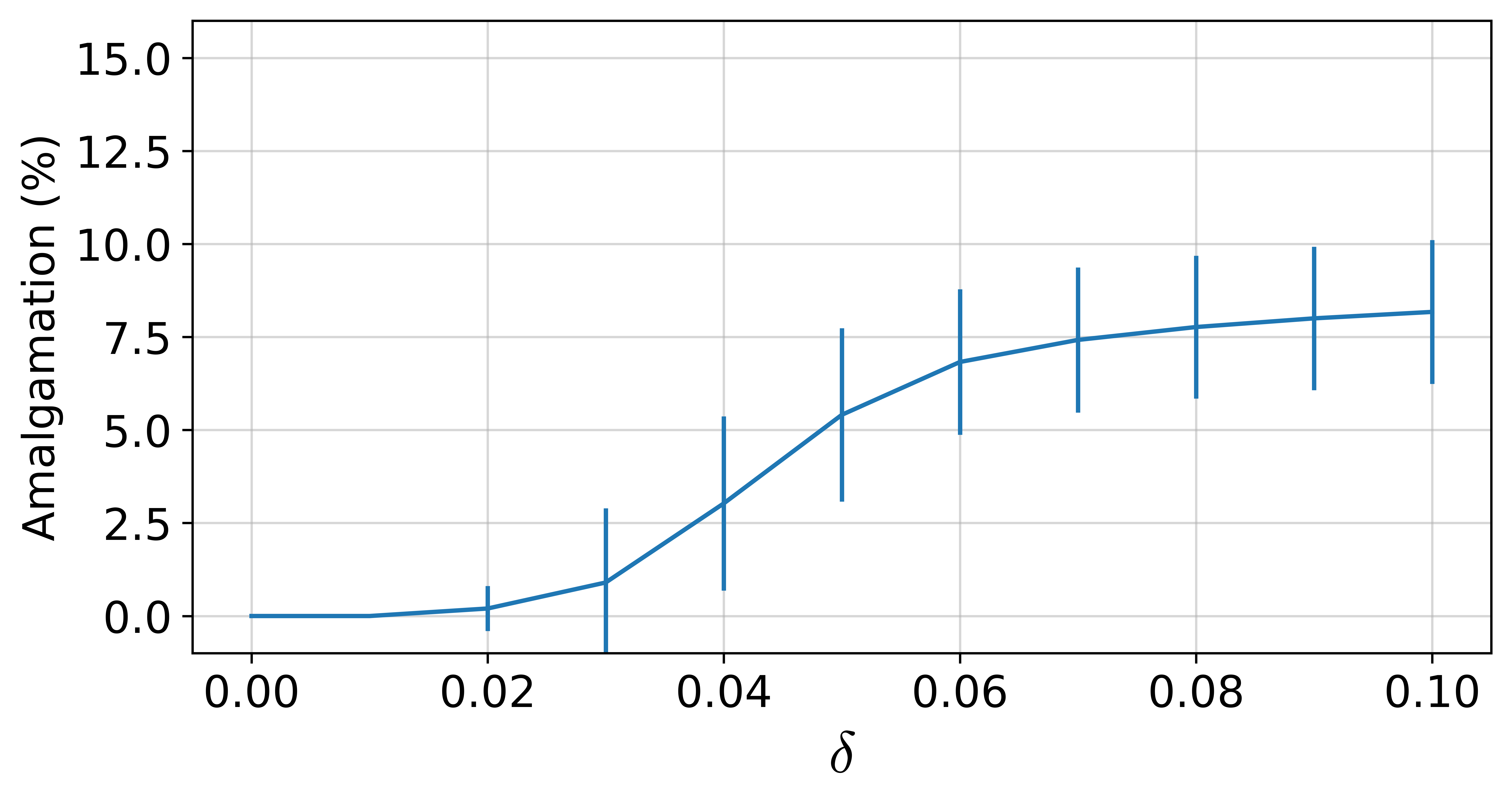
(a) Amalgamation under different $\delta$

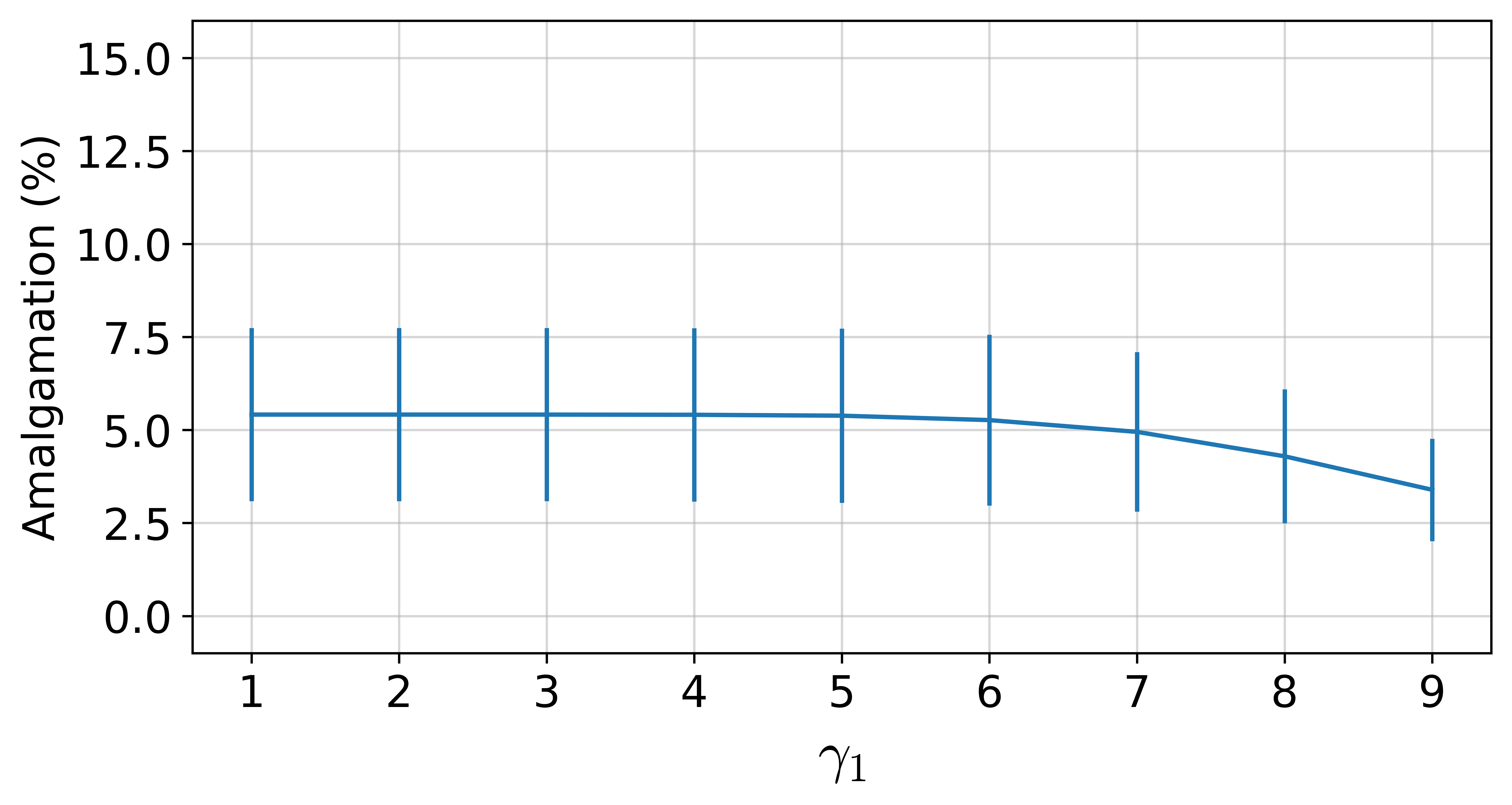
(b) Amalgamation under different $\gamma_{1}$

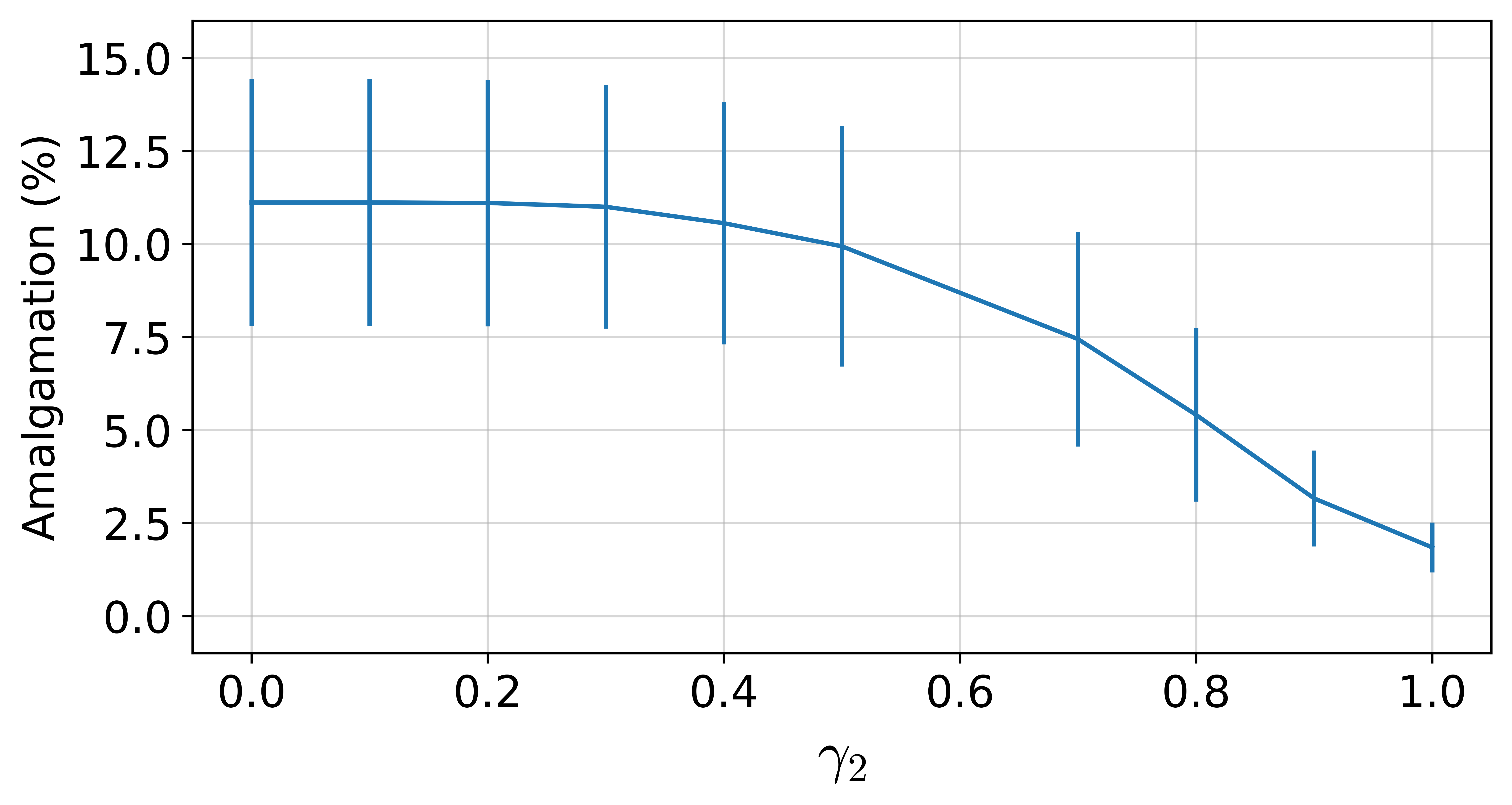
(c) Amalgamation under different $\gamma_{2}$

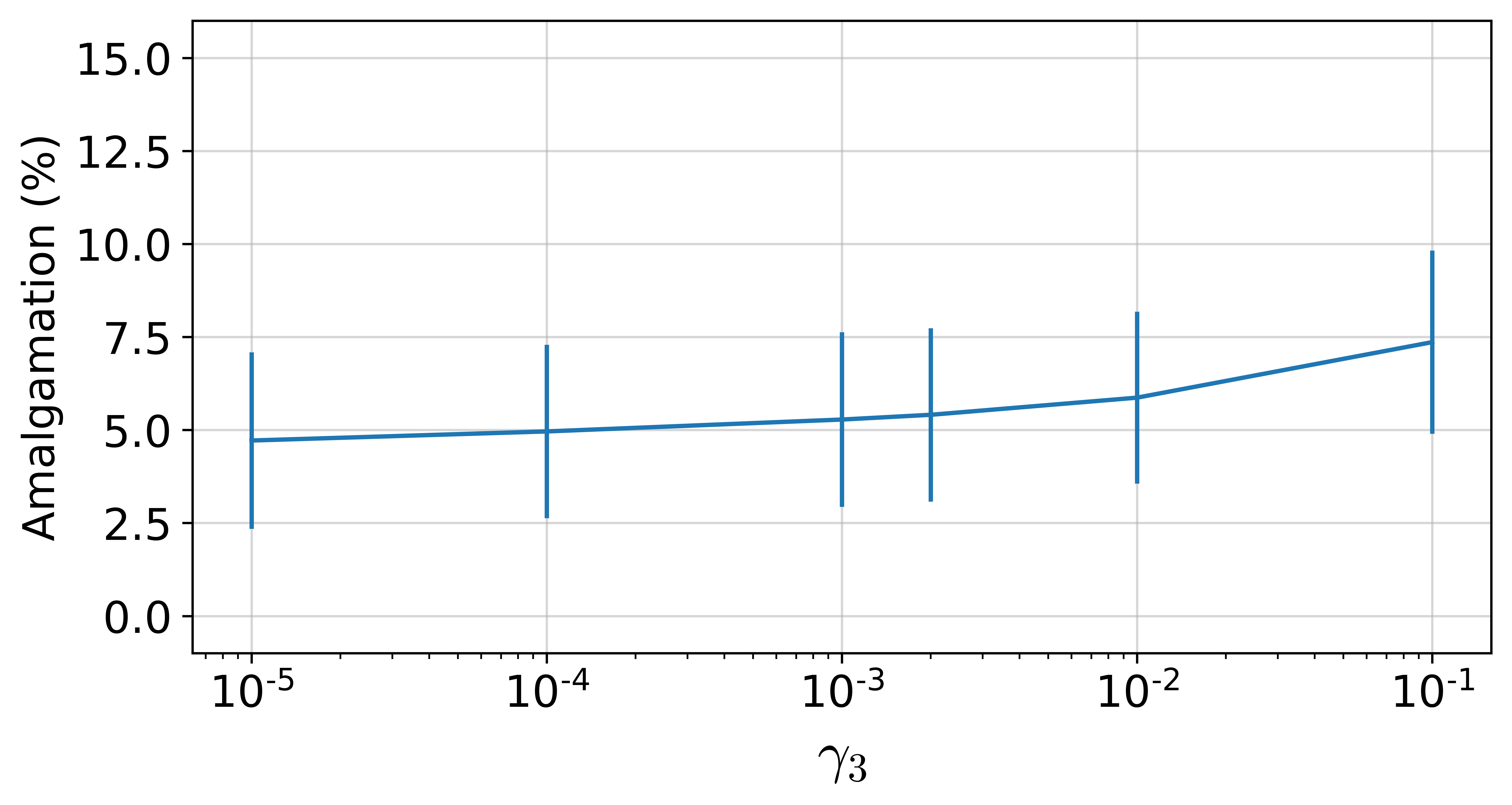
(d) Amalgamation under different $\gamma_{3}$

Figure 11: Impact of parameters on amalgamation.

Naturally, correlations between the metrics constrained by different parameters means that varying one parameter while maintaining others at conservative levels may not have a significant effect. In particular, the construction of the set $\mathcal{A}$ relies on the intersection of the two metrics controlled by $\gamma_{1}$ and $\gamma_{2}$. When $\gamma_{2}$ is set to a conservative threshold, this gives the impression that $\gamma_{1}$ does not impact the amalgamated set. Figures 12(a) and 12(b) show the individual impact of $\gamma_{1}$ and $\gamma_{2}$ when the other parameter does not constraint the set of amalgamated points, i.e. when $gamma_{2}=0$ and $gamma_{1}=0$, respectively. This shows that, while both metrics may constrain the set $\mathcal{A}$, in our experiments the amalgamation set is more influenced by $\gamma_{2}$. This can be explained by the fact that there do not seem to be points for which the influence is dominated by less than four experts.

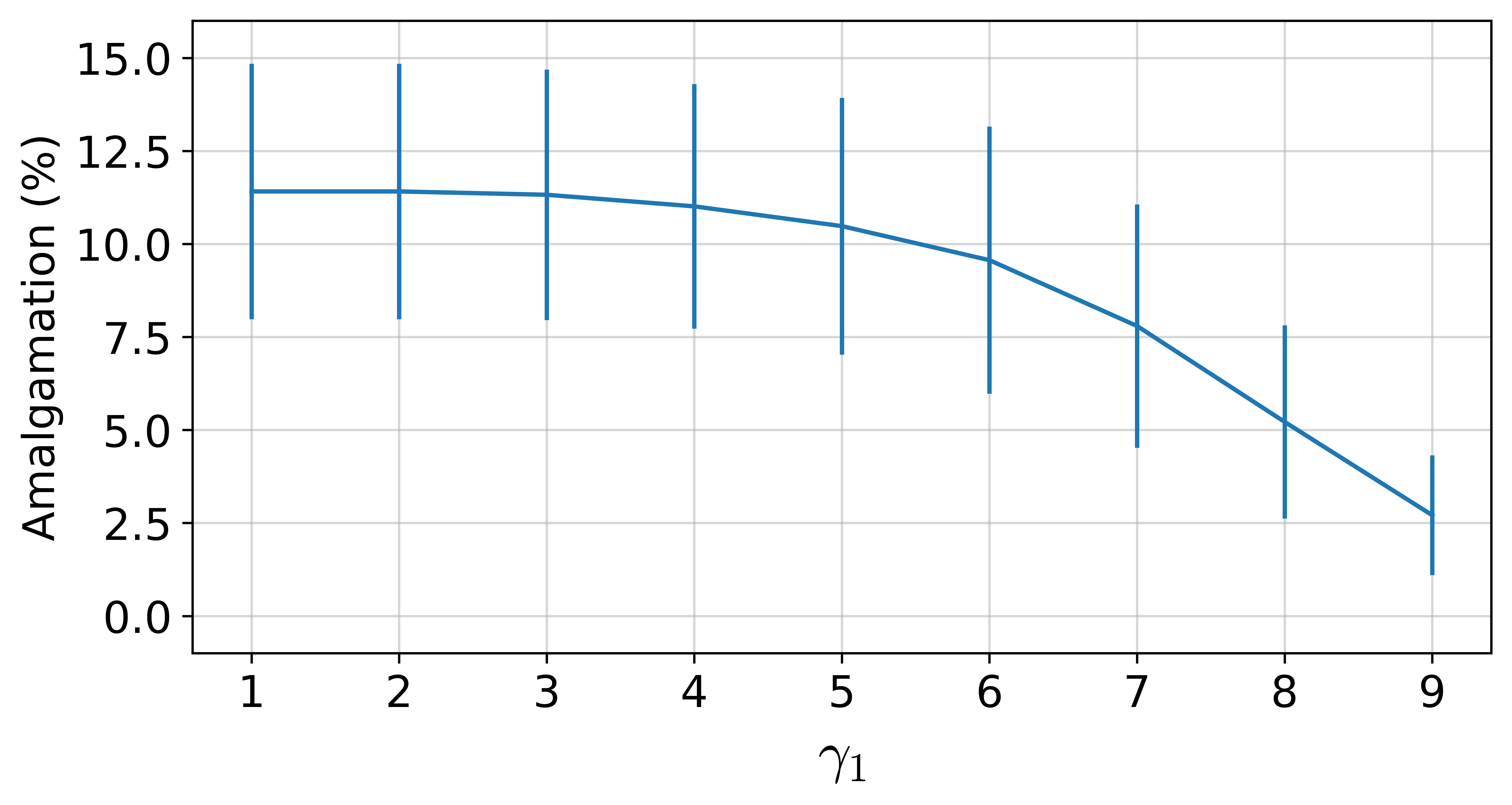
(a) Individual impact of $\gamma_{1}$

(b) Individual impact of $\gamma_{2}$

Figure 12: Individual impact of parameters on amalgamation.

Finally, we show the method’s performance when choosing more extreme sets of parameters, illustrating performance with overly relaxed constraints and overly conservative ones. Figures 13(a) and 13(b) shows the precision evolution for the quadruplets $(\delta,\gamma_{1},\gamma_{2},\gamma_{3})=(0.05,2,0.6,0.002)$ —more relaxed— and $(0.05,6,0.9,0.002)$ —more conservative. This shows how including more of the human expertise results in a model less discriminative for $Y$, but improves the prediction of complementary outcomes. Conversely, relying less on humans lead to better discrimination on $Y$ but hurts performance on the two other outcomes. Across all settings, $\hat{f}_{\mathcal{A}}$ performs significantly better than $\hat{f}_{h}$ with respect to out-of-home placement, and significantly better that $\hat{f}_{Y}$ with respect to services and substantiation.

(a) With relaxed parameters.

(b) With conservative parameters.

Figure 13: Precision on child maltreatment risk assessment for top p% highest scored screened-in cases by neural network model.

References

- Adamson and Welch, (2019) Adamson, A. S. and Welch, H. G. (2019). Machine learning and the cancer-diagnosis problem — no gold standard. New England Journal of Medicine, 381(24):2285–2287. PMID: 31826337.
- Allegheny County Department of Human Services, (2020) Allegheny County Department of Human Services (2020). Allegheny family screening tool. The Allegheny Family Screening Tool.
- Amirkhani and Rahmati, (2014) Amirkhani, H. and Rahmati, M. (2014). Agreement/disagreement based crowd labeling. Applied intelligence, 41(1):212–222.
- Argall et al., (2009) Argall, B. D., Chernova, S., Veloso, M., and Browning, B. (2009). A survey of robot learning from demonstration. Robotics and autonomous systems, 57(5):469–483.
- Banerjee et al., (1999) Banerjee, M., Capozzoli, M., McSweeney, L., and Sinha, D. (1999). Beyond kappa: A review of interrater agreement measures. Canadian journal of statistics, 27(1):3–23.
- Barocas and Selbst, (2016) Barocas, S. and Selbst, A. D. (2016). Big data’s disparate impact. California Law Review, 104:671.
- Bhatt et al., (2021) Bhatt, U., Antorán, J., Zhang, Y., Liao, Q. V., Sattigeri, P., Fogliato, R., Melançon, G., Krishnan, R., Stanley, J., Tickoo, O., et al. (2021). Uncertainty as a form of transparency: Measuring, communicating, and using uncertainty. In Proceedings of the 2021 AAAI/ACM Conference on AI, Ethics, and Society, pages 401–413.
- Bickel et al., (1993) Bickel, P. J., Klaassen, C. A., Bickel, P. J., Ritov, Y., Klaassen, J., Wellner, J. A., and Ritov, Y. (1993). Efficient and adaptive estimation for semiparametric models, volume 4. Johns Hopkins University Press Baltimore.
- Broderick et al., (2020) Broderick, T., Giordano, R., and Meager, R. (2020). An automatic finite-sample robustness metric: When can dropping a little data make a big difference? arXiv preprint arXiv:2011.14999.
- Brown et al., (2019) Brown, A., Chouldechova, A., Putnam-Hornstein, E., Tobin, A., and Vaithianathan, R. (2019). Toward algorithmic accountability in public services: A qualitative study of affected community perspectives on algorithmic decision-making in child welfare services. In Proceedings of the 2019 CHI Conference on Human Factors in Computing Systems, pages 1–12.
- Buçinca et al., (2021) Buçinca, Z., Malaya, M. B., and Gajos, K. Z. (2021). To trust or to think: cognitive forcing functions can reduce overreliance on ai in ai-assisted decision-making. Proceedings of the ACM on Human-Computer Interaction, 5(CSCW1):1–21.
- Calinon, (2009) Calinon, S. (2009). Robot programming by demonstration. EPFL Press.
- Caruana et al., (2015) Caruana, R., Lou, Y., Gehrke, J., Koch, P., Sturm, M., and Elhadad, N. (2015). Intelligible models for healthcare: Predicting pneumonia risk and hospital 30-day readmission. In Proceedings of the 21th ACM SIGKDD international conference on knowledge discovery and data mining, pages 1721–1730.
- Chalfin et al., (2016) Chalfin, A., Danieli, O., Hillis, A., Jelveh, Z., Luca, M., Ludwig, J., and Mullainathan, S. (2016). Productivity and selection of human capital with machine learning. American Economic Review, 106(5):124–27.
- Cheng et al., (2022) Cheng, H.-F., Stapleton, L., Kawakami, A., Sivaraman, V., Cheng, Y., Qing, D., Perer, A., Holstein, K., Wu, Z. S., and Zhu, H. (2022). How child welfare workers reduce racial disparities in algorithmic decisions. In CHI Conference on Human Factors in Computing Systems, pages 1–22.
- Chiang and Yin, (2021) Chiang, C.-W. and Yin, M. (2021). You’d better stop! understanding human reliance on machine learning models under covariate shift. In 13th ACM Web Science Conference 2021, pages 120–129.
- Chouldechova, (2017) Chouldechova, A. (2017). Fair prediction with disparate impact: A study of bias in recidivism prediction instruments. Big Data, Special issue on Social and Technical Trade-Offs.
- Chouldechova et al., (2018) Chouldechova, A., Benavides-Prado, D., Fialko, O., and Vaithianathan, R. (2018). A case study of algorithm-assisted decision making in child maltreatment hotline screening decisions. In Conference on Fairness, Accountability and Transparency, pages 134–148.
- Cohen, (1960) Cohen, J. (1960). A coefficient of agreement for nominal scales. Educational and psychological measurement, 20(1):37–46.
- Cook, (1986) Cook, R. D. (1986). Assessment of local influence. Journal of the Royal Statistical Society: Series B (Methodological), 48(2):133–155.
- Cortes et al., (2016) Cortes, C., DeSalvo, G., and Mohri, M. (2016). Learning with rejection. In International Conference on Algorithmic Learning Theory, pages 67–82. Springer.
- Dai et al., (2021) Dai, J., Fazelpour, S., and Lipton, Z. (2021). Fair machine learning under partial compliance. In Proceedings of the 2021 AAAI/ACM Conference on AI, Ethics, and Society, pages 55–65.
- D’Amour et al., (2020) D’Amour, A., Srinivasan, H., Atwood, J., Baljekar, P., Sculley, D., and Halpern, Y. (2020). Fairness is not static: deeper understanding of long term fairness via simulation studies. In Proceedings of the 2020 Conference on Fairness, Accountability, and Transparency, pages 525–534.
- Das et al., (2007) Das, A. S., Datar, M., Garg, A., and Rajaram, S. (2007). Google news personalization: scalable online collaborative filtering. In Proceedings of the 16th international conference on World Wide Web, pages 271–280.
- Davani et al., (2022) Davani, A. M., Díaz, M., and Prabhakaran, V. (2022). Dealing with disagreements: Looking beyond the majority vote in subjective annotations. Transactions of the Association for Computational Linguistics, 10:92–110.
- Dawes et al., (1989) Dawes, R. M., Faust, D., and Meehl, P. E. (1989). Clinical versus actuarial judgment. Science, 243(4899):1668–1674.
- De-Arteaga et al., (2020) De-Arteaga, M., Fogliato, R., and Chouldechova, A. (2020). A case for humans-in-the-loop: Decisions in the presence of erroneous algorithmic scores. In Proceedings of the 2020 CHI Conference on Human Factors in Computing Systems, pages 1–12.
- Dietvorst et al., (2015) Dietvorst, B. J., Simmons, J. P., and Massey, C. (2015). Algorithm aversion: People erroneously avoid algorithms after seeing them err. Journal of Experimental Psychology: General, 144(1):114.
- Dietvorst et al., (2018) Dietvorst, B. J., Simmons, J. P., and Massey, C. (2018). Overcoming algorithm aversion: People will use imperfect algorithms if they can (even slightly) modify them. Management Science, 64(3):1155–1170.
- Doan et al., (2011) Doan, A., Ramakrishnan, R., and Halevy, A. Y. (2011). Crowdsourcing systems on the world-wide web. Communications of the ACM, 54(4):86–96.
- Eubanks, (2018) Eubanks, V. (2018). Automating inequality: How high-tech tools profile, police, and punish the poor. St. Martin’s Press.
- Fazelpour and De-Arteaga, (2022) Fazelpour, S. and De-Arteaga, M. (2022). Diversity in sociotechnical machine learning systems. Big Data & Society, 9(1):20539517221082027.
- Fogliato et al., (2022) Fogliato, R., De-Arteaga, M., and Chouldechova, A. (2022). A case for humans-in-the-loop: Decisions in the presence of misestimated algorithmic scores. Available at SSRN 4050125.
- Fogliato et al., (2021) Fogliato, R., Xiang, A., Lipton, Z., Nagin, D., and Chouldechova, A. (2021). On the validity of arrest as a proxy for offense: Race and the likelihood of arrest for violent crimes. In Proceedings of the 2021 AAAI/ACM Conference on AI, Ethics, and Society, pages 100–111.
- Friedler et al., (2016) Friedler, S. A., Scheidegger, C., and Venkatasubramanian, S. (2016). On the (im) possibility of fairness. arXiv preprint arXiv:1609.07236.
- Geva and Saar-Tsechansky, (2020) Geva, T. and Saar-Tsechansky, M. (2020). Who is a better decision maker? data-driven expert ranking under unobserved quality. Production and Operations Management.
- Green and Chen, (2021) Green, B. and Chen, Y. (2021). Algorithmic risk assessments can alter human decision-making processes in high-stakes government contexts. Proceedings of the ACM on Human-Computer Interaction, 5(CSCW2):1–33.
- Grove et al., (2000) Grove, W. M., Zald, D. H., Lebow, B. S., Snitz, B. E., and Nelson, C. (2000). Clinical versus mechanical prediction: a meta-analysis. Psychological assessment, 12(1):19.
- Gulshan et al., (2016) Gulshan, V., Peng, L., Coram, M., Stumpe, M. C., Wu, D., Narayanaswamy, A., Venugopalan, S., Widner, K., Madams, T., Cuadros, J., et al. (2016). Development and validation of a deep learning algorithm for detection of diabetic retinopathy in retinal fundus photographs. Jama, 316(22):2402–2410.
- Gwet et al., (2002) Gwet, K. et al. (2002). Inter-rater reliability: dependency on trait prevalence and marginal homogeneity. Statistical Methods for Inter-Rater Reliability Assessment Series, 2(1):9.
- Herr and Burt, (2005) Herr, E. and Burt, L. (2005). Predicting student loan default for the university of texas at austin. Journal of Student Financial Aid, 35(2):27–49.
- Hong et al., (2018) Hong, W. S., Haimovich, A. D., and Taylor, R. A. (2018). Predicting hospital admission at emergency department triage using machine learning. PloS one, 13(7):e0201016.
- Horvitz et al., (1988) Horvitz, E. J., Breese, J. S., and Henrion, M. (1988). Decision theory in expert systems and artificial intelligence. International journal of approximate reasoning, 2(3):247–302.
- Huang et al., (2007) Huang, J., Gretton, A., Borgwardt, K. M., Schölkopf, B., and Smola, A. J. (2007). Correcting sample selection bias by unlabeled data. In Advances in Neural Information Processing Systems, pages 601–608.
- Jacobs and Wallach, (2021) Jacobs, A. Z. and Wallach, H. (2021). Measurement and fairness. In Proceedings of the 2021 ACM conference on fairness, accountability, and transparency, pages 375–385.
- Johnson et al., (2021) Johnson, A., Bulgarelli, L., Pollard, T., Celi, L. A., Mark, R., and Horng, S. (2021). Mimic-iv-ed (version 1.0).
- Kandasamy et al., (2015) Kandasamy, K., Krishnamurthy, A., Poczos, B., Wasserman, L., and Robins, J. M. (2015). Nonparametric von mises estimators for entropies, divergences and mutual informations. In Advances in Neural Information Processing Systems 28, pages 397–405.
- Kennedy, (2016) Kennedy, E. H. (2016). Semiparametric theory and empirical processes in causal inference. In Statistical Causal Inferences and Their Applications in Public Health Research, pages 141–167. Springer.
- Khandani et al., (2010) Khandani, A. E., Kim, A. J., and Lo, A. W. (2010). Consumer credit-risk models via machine-learning algorithms. Journal of Banking & Finance, 34(11):2767–2787.
- Kleinberg et al., (2017) Kleinberg, J., Lakkaraju, H., Leskovec, J., Ludwig, J., and Mullainathan, S. (2017). Human decisions and machine predictions. Technical report, National Bureau of Economic Research.
- Koh and Liang, (2017) Koh, P. W. and Liang, P. (2017). Understanding black-box predictions via influence functions. In Proceedings of the 34th International Conference on Machine Learning-Volume 70, pages 1885–1894. JMLR. org.
- Koh et al., (2019) Koh, P. W. W., Ang, K.-S., Teo, H., and Liang, P. S. (2019). On the accuracy of influence functions for measuring group effects. In Advances in Neural Information Processing Systems, pages 5254–5264.
- Lakkaraju et al., (2017) Lakkaraju, H., Kleinberg, J., Leskovec, J., Ludwig, J., and Mullainathan, S. (2017). The selective labels problem: Evaluating algorithmic predictions in the presence of unobservables. In Proceedings of the 23rd ACM SIGKDD International Conference on Knowledge Discovery and Data Mining, pages 275–284. ACM.
- Lebovitz et al., (2019) Lebovitz, S., Levina, N., and Lifshitz-Assaf, H. (2019). Doubting the diagnosis: How artificial intelligence increases ambiguity during professional decision making. Available at SSRN 3480593.
- Little and Rubin, (2014) Little, R. J. and Rubin, D. B. (2014). Statistical analysis with missing data. John Wiley & Sons.
- Luca et al., (2016) Luca, M., Kleinberg, J., and Mullainathan, S. (2016). Algorithms need managers, too. Harvard business review, 94(1):20.
- Madras et al., (2018) Madras, D., Pitassi, T., and Zemel, R. (2018). Predict responsibly: Improving fairness and accuracy by learning to defer. In Advances in Neural Information Processing Systems 31, pages 6147–6157.
- McKinney et al., (2020) McKinney, S. M., Sieniek, M., Godbole, V., Godwin, J., Antropova, N., Ashrafian, H., Back, T., Chesus, M., Corrado, G. C., Darzi, A., et al. (2020). International evaluation of an ai system for breast cancer screening. Nature, 577(7788):89–94.
- Meehl, (1954) Meehl, P. E. (1954). Clinical versus statistical prediction: A theoretical analysis and a review of the evidence. In In Proceedings of the 1955 Invitational Conference on Testing Problems, pages 136–141. University of Minnesota Press.
- Meyer et al., (2014) Meyer, G., Adomavicius, G., Johnson, P. E., Elidrisi, M., Rush, W. A., Sperl-Hillen, J. M., and O’Connor, P. J. (2014). A machine learning approach to improving dynamic decision making. Information Systems Research, 25(2):239–263.
- Mullainathan and Obermeyer, (2017) Mullainathan, S. and Obermeyer, Z. (2017). Does machine learning automate moral hazard and error? American Economic Review, 107(5):476–80.
- Obermeyer et al., (2019) Obermeyer, Z., Powers, B., Vogeli, C., and Mullainathan, S. (2019). Dissecting racial bias in an algorithm used to manage the health of populations. Science, 366(6464):447–453.
- Passi and Barocas, (2019) Passi, S. and Barocas, S. (2019). Problem formulation and fairness. In Proceedings of the Conference on Fairness, Accountability, and Transparency, pages 39–48.
- Raita et al., (2019) Raita, Y., Goto, T., Faridi, M. K., Brown, D. F., Camargo, C. A., and Hasegawa, K. (2019). Emergency department triage prediction of clinical outcomes using machine learning models. Critical care, 23(1):1–13.
- Robins et al., (2000) Robins, J. M., Hernan, M. A., and Brumback, B. (2000). Marginal structural models and causal inference in epidemiology.
- Saxena et al., (2020) Saxena, D., Badillo-Urquiola, K., Wisniewski, P. J., and Guha, S. (2020). A human-centered review of algorithms used within the us child welfare system. In Proceedings of the 2020 CHI Conference on Human Factors in Computing Systems, pages 1–15.
- Seaman and White, (2013) Seaman, S. R. and White, I. R. (2013). Review of inverse probability weighting for dealing with missing data. Statistical methods in medical research, 22(3):278–295.
- Shanteau, (1992) Shanteau, J. (1992). Competence in experts: The role of task characteristics. Organizational behavior and human decision processes, 53(2):252–266.
- Shanteau, (2015) Shanteau, J. (2015). Why task domains (still) matter for understanding expertise. Journal of Applied Research in Memory and Cognition, 4(3):169–175.
- Sharda et al., (1988) Sharda, R., Barr, S. H., and MCDonnell, J. C. (1988). Decision support system effectiveness: a review and an empirical test. Management Science, 34(2):139–159.
- Snow et al., (2008) Snow, R., O’Connor, B., Jurafsky, D., and Ng, A. Y. (2008). Cheap and fast—but is it good?: evaluating non-expert annotations for natural language tasks. In Proceedings of the conference on empirical methods in natural language processing, pages 254–263. Association for Computational Linguistics.
- Stevenson and Doleac, (2019) Stevenson, M. T. and Doleac, J. L. (2019). Algorithmic risk assessment in the hands of humans. Available at SSRN.
- Tan et al., (2010) Tan, C.-H., Teo, H.-H., and Benbasat, I. (2010). Assessing screening and evaluation decision support systems: A resource-matching approach. Information Systems Research, 21(2):305–326.
- Umesh et al., (1989) Umesh, U. N., Peterson, R. A., and Sauber, M. H. (1989). Interjudge agreement and the maximum value of kappa. Educational and Psychological Measurement, 49(4):835–850.
- U.S. Department of Health and Human Services, (2020) U.S. Department of Health and Human Services (2020). Child maltreatment 2018.
- Wang et al., (2018) Wang, J., Oh, J., Wang, H., and Wiens, J. (2018). Learning credible models. In Proceedings of the 24th ACM SIGKDD International Conference on Knowledge Discovery & Data Mining, pages 2417–2426. ACM.
- Wilder et al., (2020) Wilder, B., Horvitz, E., and Kamar, E. (2020). Learning to complement humans. In Proceedings of the 29th International Joint Conference on Artificial Intelligence, pages 1526–1533.
- Wilkinson, (2009) Wilkinson, D. (2009). The self-fulfilling prophecy in intensive care. Theoretical medicine and bioethics, 30(6):401–410.
- Yoganarasimhan, (2020) Yoganarasimhan, H. (2020). Search personalization using machine learning. Management Science, 66(3):1045–1070.
- Zadrozny, (2004) Zadrozny, B. (2004). Learning and evaluating classifiers under sample selection bias. In Proceedings of the twenty-first international conference on Machine learning, page 114. ACM.
- Zhang et al., (2016) Zhang, J., Wu, X., and Sheng, V. S. (2016). Learning from crowdsourced labeled data: a survey. Artificial Intelligence Review, 46(4):543–576.