Abstract

We review the current status of the research on effective nonlocal NJL-like chiral quark models with separable interactions, focusing on the application of this approach to the description of the properties of hadronic and quark matter under extreme conditions. The analysis includes the predictions for various hadron properties in vacuum, as well as the study of the features of deconfinement and chiral restoration phase transitions for systems at finite temperature and/or density. We also address other related subjects, such as the study of phase transitions for imaginary chemical potentials, the possible existence of inhomogeneous phase regions, the presence of color superconductivity, the effects produced by strong external magnetic fields, and the application to the description of compact stellar objects.

xx 1 5 Strong-interaction matter under extreme conditions from chiral quark models with nonlocal separable interactions D. Gómez Dumm^1,∗, J.P. Carlomagno¹ and N.N. Scoccola ^2,3 Firstname Lastname, Firstname Lastname and Firstname Lastname Correspondence: dumm@fisica.unlp.edu.ar

1 Introduction

The detailed understanding of the behavior of strong-interaction matter under extreme conditions of temperature and/or density has attracted great attention in the past decades. This is not only an issue of fundamental interest but has also important implications on the description of the early evolution of the Universe Schwarz:2003du and on the study of the interior of compact stellar objects Page:2006ud ; Lattimer:2015nhk . It is widely believed that as the temperature $T$ and/or the baryon chemical potential $\mu_{B}$ increase, one finds a transition from a hadronic phase, in which chiral symmetry is broken and quarks are confined, to a phase in which chiral symmetry is partially restored and/or quarks are deconfined. In fact, the problems of how and when these transitions occur have been intensively investigated, both from theoretical and experimental points of view. On the experimental side, the properties of strong-interaction matter are being studied by large research programs at the Relativistic Heavy Ion Collider (RHIC, Brookhaven), as well as at the Large Hadron Collider (LHC) and the Super Proton Synchrotron (SPS) in CERN. Experiments at these facilities allow for the exploration of the properties of hot and dense matter created in collisions of ultra-relativistic heavy ions Braun-Munzinger:2015hba ; Busza:2018rrf . The quark-gluon plasma produced at high energies at RHIC and LHC contains almost equal amounts of matter and antimatter, and serves to probe the region of high temperatures and low chemical potentials in the $\mu_{B}-T$ phase diagram. In addition, the variation of collision energies at RHIC through the beam energy scan (BES) program Bzdak:2019pkr has enabled the systematical exploration of the phase structure of strong-interaction matter at nonzero chemical potential. These studies will be complemented in the next future by experiments at the facilities FAIR in Darmstadt and NICA in Dubna, reaching in this way experimental access to the bulk of the phase diagram. It should be stressed that additional information about the behavior of dense quark matter systems can be provided by the wealth of data on the properties of compact stars, obtained through neutron star and gravitational wave observations from e.g. the Neutron Star Interior Composition Explorer (NICER), gravitational-wave observatories such as LIGO or VIRGO, etc. Baym:2017whm . From the theoretical point of view, addressing this subject requires to deal with quantum chromodynamics (QCD) in nonperturbative regimes. One way to cope with this problem is through lattice QCD (LQCD) calculations Karsch:2001vs ; Ding:2015ona . However, in spite of the significant improvements produced over the years, this ab initio approach is not yet able to provide a full understanding of the QCD phase diagram, owing to the well known “sign problem” Karsch:2001cy that affects LQCD calculations at finite chemical potential. Thus, our present theoretical understanding of the strong-interaction matter phase diagram largely relies on the use of effective models of low energy QCD that show consistency with LQCD results at $\mu_{B}\simeq 0$, and can be extrapolated into regions not accessible by lattice calculation techniques.

One of the most popular approaches to an effective description of QCD interactions is the quark version of the Nambu$-$Jona-Lasinio (NJL) model Nambu:1961tp ; Nambu:1961fr , in which quark fields interact through local four-point vertices that satisfy chiral symmetry constraints. This type of model provides a mechanism for the spontaneous breakdown of chiral symmetry and the formation of a quark condensate, and has been widely used to describe the features of chiral restoration at finite temperature and/or density Vogl:1991qt ; Klevansky:1992qe ; Hatsuda:1994pi . Thermodynamic aspects of confinement, while absent in the original NJL model, can be implemented by a synthesis with Polyakov-loop (PL) dynamics Polyakov:1978vu ; Fukushima:2017csk . The resulting Polyakov-Nambu-Jona-Lasinio (PNJL) model Meisinger:1995ih ; Fukushima:2003fw ; Megias:2004hj ; Ratti:2005jh ; Roessner:2006xn ; Mukherjee:2006hq ; Sasaki:2006ww allows one to study the chiral and deconfinement transitions in a common framework.

As an improvement over local models, chiral quark models that include nonlocal separable interactions have also been considered Schmidt:1994di ; Burden:1996nh ; Bowler:1994ir ; Ripka:1997zb . Since these approaches can be viewed as nonlocal extensions of the NJL model, here we denote them generically as “nonlocal NJL” (nlNJL) models. In fact, nonlocal interactions arise naturally in the context of several successful approaches to low-energy quark dynamics Schafer:1996wv ; Roberts:1994dr , and lead to a momentum dependence in quark propagators that can be made consistent Noguera:2005ej ; Noguera:2008cm with lattice results Parappilly:2005ei ; Furui:2006ks . Moreover, it can be seen that nonlocal extensions of the NJL model do not show some of the known inconveniences that can be found in the local theory. Well-behaved nonlocal form factors can regularize loop integrals in such a way that anomalies are preserved RuizArriola:1998zi and charges are properly quantized. In addition, one can avoid the introduction of various sharp cutoffs to deal with higher order loop integrals Blaschke:1995gr ; Plant:2000ty , improving in this way the predictive power of the models. At the same time, the separable character of the interactions makes possible to keep much of the simplicity of the standard NJL model, in comparison with more rigorous analytical approaches to nonperturbative QCD. Various applications of nlNJL models to the description of hadron properties at zero temperature and density can be found e.g. in Refs. Plant:1997jr ; Broniowski:1999dm ; Praszalowicz:2001wy ; Praszalowicz:2001pi ; Praszalowicz:2003pr ; Dorokhov:2003kf ; Kotko:2008gy ; Kotko:2009ij ; Kotko:2009mb ; Nam:2012vm ; Nam:2017gzm ; GomezDumm:2012qh ; Dumm:2013zoa ; Golli:1998rf ; Broniowski:2001cx ; Rezaeian:2004nf . In addition, this type of model has been applied to the description of the chiral restoration transition at finite temperature and/or density Szczerbinska:1999iz ; Blaschke:2000gd ; General:2000zx ; GomezDumm:2001fz ; GomezDumm:2004sr . The coupling of the quarks to the PL in the framework of nlNJL models gives rise to the so-called nonlocal Polyakov$-$Nambu$-$Jona-Lasinio (nlPNJL) models Blaschke:2007np ; Contrera:2007wu ; Hell:2008cc , in which quarks move in a background color field and interact through covariant nonlocal chirally symmetric couplings. It has been found that, under certain conditions, it is possible to derive the main features of nlPNJL models starting directly from QCD Kondo:2010ts .

The aim of this article is to present an overview of the existing results obtained within nonlocal NJL-like models concerning the description of hadronic and quark matter at both zero and finite temperature and/or density. The paper is organized as follows. In Sec. 2 we introduce a two-flavor nlNJL model and discuss its main theoretical features. We also study the extension of this approach to nonzero temperature and chemical potential, including the coupling of fermions to the Polyakov loop. Then, after introducing some possible model parameterizations, results for the thermodynamics of strong-interaction matter, as well as for the corresponding phase diagram both for real and imaginary quark chemical potentials, are presented and discussed. We finish this section by quoting some results for the thermal dependence of various scalar and pseudoscalar meson properties. In Sec. 3, the inclusion of explicit vector and axial vector interactions in the context of two flavor nlNJL models is considered, analyzing their impact on the corresponding phenomenological predictions. In Sec. 4 we analyze the extension of the above introduced nlPNJL model to $N_{f}=3$ flavors, incorporating a dynamical strange quark. This requires the inclusion of explicit flavor symmetry breaking terms to account for the relatively large $s$-quark mass and also the addition of a flavor mixing term related to the $U(1)_{A}$ anomaly. After describing the main features of this three-flavor nlPNJL model, results for the thermal dependence of various quantities as well as predictions for the phase diagram are given. In Sec. 5 we discuss some further developments and applications of nlPNJL models. These include the description of superconducting phases, the application to the physics of compact stars, the study of the existence of inhomogeneous phases and the analysis of the effects of external strong magnetic fields on hadron properties and phase transitions. Finally, in Sec. 6 we present our conclusions. We also add a brief appendix that includes some conventions and basic formulae.

2 Two-flavor nonlocal NJL models

In this section we review the features of nlNJL models that include just the two lightest quark flavors, $u$ and $d$. We begin by addressing the analysis of model properties in vacuum. Then we consider systems at finite temperature and chemical potential, discussing the predictions for thermodynamic properties and the characteristics of phase transitions.

2.1 Two-flavor nlNJL model at vanishing temperature and chemical potential

2.1.1 Effective action

We start by studying the features of nlNJL models at zero temperature and chemical potential. Let us consider the Euclidean action given by Noguera:2008cm

$$S_{E}\ =\ \int d^{4}x\ \left\{\bar{\psi}(x)\left(-i\hbox to0.0pt{/\hss}\partial+m_{c}\right)\psi(x)-\frac{G_{S}}{2}\Big{[}j_{S}(x)j_{S}(x)+\vec{\jmath}_{P}(x)\cdot\vec{\jmath}_{P}(x)+j_{R}(x)j_{R}(x)\Big{]}\right\}\ ,$$ (1)

where $\psi$ stands for the $u$, $d$ quark field doublet and $m_{c}$ is the current quark mass. Throughout this article we will work in the isospin limit, thus we assume the current mass to be the same for $u$ and $d$ quarks. The nonlocal character of the model arises from the quark-antiquark currents $j_{S}(x)$, $j_{P}(x)$ and $j_{R}(x)$, given by

$$j_{S}(x) = \int d^{4}z\;\mathcal{G}(z)\,\bar{\psi}\left(x+\frac{z}{2}\right)\psi\left(x-\frac{z}{2}\right)\ ,$$

$$\vec{\jmath}_{P}(x) = \int d^{4}z\;\mathcal{G}(z)\,\bar{\psi}\left(x+\frac{z}{2}\right)i\,\gamma_{5}\,\vec{\tau}\,\psi\left(x-\frac{z}{2}\right)\ ,$$

$$j_{R}(x) = \int d^{4}z\ \mathcal{F}(z)\ \bar{\psi}\left(x+\frac{z}{2}\right)\ \frac{i{\overleftrightarrow{\hbox to0.0pt{/\hss}\partial}}}{2\ \varkappa_{p}}\ \psi\left(x-\frac{z}{2}\right)\ ,$$ (2)

where $u(x^{\prime}){\overleftrightarrow{\partial}}v(x)=u(x^{\prime})\partial_{x}v(x)-\partial_{x^{\prime}}u(x^{\prime})v(x)$. The functions $\mathcal{G}(z)$ and $\mathcal{F}(z)$ in Eq. (2) are effective covariant form factors that encode the effects of the underlying low energy QCD interactions. Chiral invariance requires that the quark currents $j_{S}(x)$ and $j_{P\,a}(x)$, $a=1,2,3$, carry the same form factor $\mathcal{G}(z)$, while the $j_{R}(x)j_{R}(x)$ coupling is found to be self-invariant under chiral transformations. The local version of the (quark-level) NJL model is obtained by taking $\mathcal{G}(z)=\delta^{(4)}(z)$ and $\mathcal{F}(z)=0$, together with a proper regularization prescription.

It can be shown that the presence of the nonlocal form factor in the scalar current $j_{S}(x)$ leads to a momentum-dependent quark effective mass, as expected from lattice QCD calculations Parappilly:2005ei . On the other hand, the coupling involving the current $j_{R}(x)$ is related to the quark wave function renormalization (WFR). Whereas in a local theory this coupling would simply lead —at the mean field level— to a redefinition of fermion fields, in the nonlocal scheme it leads to a momentum-dependent WFR of the quark propagator, in consistency with LQCD analyses Parappilly:2005ei . To simplify the notation, the same coupling constant $G_{S}$ has been taken for all interaction terms. Note, however, that the relative strength between the $j_{R}(x)j_{R}(x)$ coupling and the other terms is controlled by the mass parameter $\varkappa_{p}$ in Eq. (2). The form factors ${\cal G}(z)$ and ${\cal F}(z)$ are dimensionless and can be normalized to ${\cal G}(0)={\cal F}(0)=1$ without loss of generality.

It is worth stressing that the currents in Eq. (2) are not to be directly identified with the color octet quark currents entering the QCD Lagrangian. The former are color singlet quantities that contain part of the effective gluon mediated interaction, and are introduced as a convenient way of expressing the interaction terms in a chiral quark model. In addition, it is important to notice that the couplings in Eq. (1) are not intended to be the most general nonlocal current-current interactions compatible with QCD symmetries. In fact, this is just the simplest model that, within the mean field approximation, leads to an effective quark propagator including a momentum-dependent wave function renormalization $Z(p)$ and a momentum-dependent mass $M(p)$. Clearly, other quark-antiquark and/or quark-quark current interactions can be added in order to properly account for the description of vector mesons physics, color superconductivity effects, etc. Some possible extensions of the model will be discussed in the next sections of this article. In addition, it is worth taking into account that in Eqs. (2) we have chosen a particular way of introducing nonlocal form factors in the quark currents. As discussed in Refs. Schmidt:1994di ; Burden:1996nh , this scheme is based on a separable approach to the effective one gluon exchange (OGE) interactions. Alternatively, a scheme based on the features of the instanton liquid model (ILM) has been introduced in Ref. Bowler:1994ir . In that approach a nonlocal form factor is associated to each quark field, in such a way that e.g. the scalar nonlocal current $j_{S}(x)$ reads

$$j_{S}^{\mathrm{ILM}}(x)\ =\ \int d^{4}y\,d^{4}z\ \mathcal{R}(y-x)\,\mathcal{R}(x-z)\ \bar{\psi}\left(y\right)\psi\left(z\right)\ .$$ (3)

Whereas both OGE and ILM-inspired schemes are equivalent at the mean- field level, the treatment of fluctuations is somewhat different. A comparison of both approaches can be found in Ref. GomezDumm:2006vz . In this review we mostly concentrate on the OGE-based scheme, which is the more widely used to study the behavior of quark and hadronic matter at finite temperature and/or density. However, when possible, references to the results obtained within the alternative ILM-based scheme will be included.

In order to deal with meson degrees of freedom, it is convenient to perform a standard bosonization of the theory given by the action in Eq. (1). This can be done by considering the corresponding partition function $\mathcal{Z}=\int{\rm D}\bar{\psi}\,{\rm D}\psi\,\exp(-S_{E})$, and introducing auxiliary fields $\sigma_{1}(x)$, $\sigma_{2}(x)$ and $\pi_{a}(x)$, $a=1,2,3$, which account for scalar and pseudoscalar mesons. Integrating out the quark fields one gets

$$\mathcal{Z}\ =\ \int{\rm D}\sigma_{1}\,{\rm D}\sigma_{2}\ {\rm D}\vec{\pi}\ \exp\!\big{(}\!-S_{E}^{\mathrm{bos}}\big{)}\ ,$$ (4)

where the bosonized action is given by

$$S_{E}^{\mathrm{bos}}\ =\ -\ln\,\det{\cal D}+\frac{1}{2G_{S}}\int\frac{d^{4}q}{(2\pi)^{4}}\ \Big{[}\sigma_{1}(q)\ \sigma_{1}(-q)+\vec{\pi}(q)\cdot\vec{\pi}(-q)+\sigma_{2}(q)\ \sigma_{2}(-q)\Big{]}\ .$$ (5)

Here, the operator ${\cal D}$ reads, in momentum space,

$${\cal D}(p,p^{\prime}) = (\hbox to0.0pt{/\hss}p+m_{c})\,(2\pi)^{4}\,\delta^{(4)}(p-p^{\prime})+g\left(\frac{p+p^{\prime}}{2}\right)\ \Big{[}\sigma_{1}(p-p^{\prime})+i\gamma_{5}\vec{\tau}\cdot\vec{\pi}(p-p^{\prime})\Big{]}$$ (6)

$$-\ f\left(\frac{p+p^{\prime}}{2}\right)\ \frac{\hbox to0.0pt{/\hss}p+{\hbox to0.0pt{/\hss}p}^{\prime}}{2\ \varkappa_{p}}\ \sigma_{2}(p-p^{\prime})\ ,$$

where $g(p)$ and $f(p)$ stand for Fourier transforms of the form factors $\mathcal{G}(z)$ and $\mathcal{F}(z)$, namely

$$g(p)\ =\ \int d^{4}z\ e^{-ip\cdot z}\ \mathcal{G}(z)\ ,\qquad\qquad f(p)\ =\ \int d^{4}z\ e^{-ip\cdot z}\ \mathcal{F}(z)\ .$$ (7)

Note that Lorentz invariance implies that they can only be functions of $p^{2}$.

Now it is assumed that the fields $\sigma_{1}$ and $\sigma_{2}$ have nontrivial translational invariant mean field values $\bar{\sigma}_{1}$ and $\varkappa_{p}\,\bar{\sigma}_{2}$, while the mean field values of the pseudoscalar fields $\pi_{i}$ are taken to be zero. Thus, one can write

$$\sigma_{1}(x)\ =\ \bar{\sigma}_{1}+\delta\sigma_{1}(x)\ ,\qquad\sigma_{2}(x)\ =\ \varkappa_{p}\ \bar{\sigma}_{2}+\delta\sigma_{2}(x)\ ,\qquad\vec{\pi}(x)\ =\ \delta\vec{\pi}(x)\ .$$ (8)

A more general case, in which the bosonic fields are expanded around inhomogeneous ground states, is considered in Sec. 5.3. Replacing in the bosonized effective action, and expanding in powers of the meson fluctuations $\delta\sigma_{1}$, $\delta\sigma_{2}$ and $\delta\vec{\pi}$, one gets

$$S_{E}^{\mathrm{bos}}\ =\ S_{E}^{\mathrm{MFA}}\,+\,S_{E}^{\mathrm{quad}}\,+\ \dots$$ (9)

The mean field action per unit volume reads Noguera:2008cm

$$\frac{S_{E}^{\mathrm{MFA}}}{V^{(4)}}\ =\ -\,2N_{c}\int\frac{d^{4}p}{(2\pi)^{4}}\ \mbox{tr}\,\ln\mathcal{D}_{0}(p)\,+\,\frac{\bar{\sigma}_{1}^{2}}{2G_{S}}\,+\,\frac{\varkappa_{p}^{2}\ \bar{\sigma}_{2}^{2}}{2G_{S}}\ ,$$ (10)

where $N_{c}=3$ is the number of colors, and the trace is taken on Dirac space. The mean field quark propagator $\mathcal{S}_{0}(p)$ is given by

$$\mathcal{S}_{0}(p)\ =\ \mathcal{D}_{0}(p)^{-1}\ =\ \frac{Z(p)}{\hbox to0.0pt{/\hss}p+M(p)}\ ,$$ (11)

with

$$Z(p)\ =\ \left(1-\bar{\sigma}_{2}\ f(p)\right)^{-1}\ ,\qquad\qquad M(p)\ =\ Z(p)\left(m_{c}+\bar{\sigma}_{1}\ g(p)\right)\ .$$ (12)

The quadratic piece in Eq. (9) can be written as

$$S_{E}^{\mathrm{quad}}\ =\ \frac{1}{2}\int\frac{d^{4}q}{(2\pi)^{4}}\left[G_{\sigma}(q^{2})\ \delta\sigma(q)\ \delta\sigma(-q)\,+\,G_{\sigma^{\prime}}(q^{2})\ \delta\sigma^{\prime}(q)\ \delta\sigma^{\prime}(-q)\,+\,G_{\pi}(q^{2})\ \delta\vec{\pi}(q)\cdot\delta\vec{\pi}(-q)\right]\ ,$$ (13)

where $\delta\sigma$ and $\delta\sigma^{\prime}$ are related to $\delta\sigma_{1}$ and $\delta\sigma_{2}$ by

$$\delta\sigma = \cos\theta\ \delta\sigma_{1}-\sin\theta\ \delta\sigma_{2}\ ,$$

$$\delta\sigma^{\prime} = \sin\theta\ \delta\sigma_{1}+\cos\theta\ \delta\sigma_{2}\ ,$$ (14)

the mixing angle $\theta$ being defined in such a way that there is no $\sigma-\sigma^{\prime}$ mixing at the level of the quadratic action. The function $G_{\pi}(q^{2})$ introduced in Eq. (13) is given by Noguera:2008cm

$$G_{\pi}(q^{2})\ =\ \frac{1}{G_{S}}-\,8\,N_{c}\int\frac{d^{4}p}{(2\pi)^{4}}\ g(p)^{2}\,\frac{Z(p^{+})Z(p^{-})}{D(p^{+})D(p^{-})}\,\left[p^{+}\cdot p^{-}+M(p^{+})M(p^{-})\right]\ ,$$ (15)

with $p^{\pm}=p\pm q/2\,$ and $D(p)=p^{2}+M(p)^{2}$. For the $\sigma-\sigma^{\prime}$ system one has

$$G_{\sigma\choose{\sigma^{\prime}}}(q^{2})\ =\ \frac{G_{\sigma_{1}\sigma_{1}}(q^{2})+G_{\sigma_{2}\sigma_{2}}(q^{2})}{2}\mp\sqrt{\left[G_{\sigma_{1}\sigma_{2}}(q^{2})\right]^{2}\!+\!\left[\frac{G_{\sigma_{1}\sigma_{1}}(q^{2})-G_{\sigma_{2}\sigma_{2}}(q^{2})}{2}\right]^{2}}\ \ ,$$ (16)

where

$$G_{\sigma_{1}\sigma_{1}}(q^{2}) = \frac{1}{G_{S}}-\,8\,N_{c}\int\frac{d^{4}p}{(2\pi)^{4}}\ g(p)^{2}\,\frac{Z(p^{+})Z(p^{-})}{D(p^{+})D(p^{-})}\left[p^{+}\cdot p^{-}-M(p^{+})M(p^{-})\right]\ ,$$

$$G_{\sigma_{2}\sigma_{2}}(q^{2}) = \frac{1}{G_{S}}+\,\frac{8\,N_{c}}{\varkappa_{p}^{2}}\ \int\frac{d^{4}p}{(2\pi)^{4}}\ p^{2}\,f(p)^{2}\,\frac{Z(p^{+})Z(p^{-})}{D(p^{+})D(p^{-})}$$

$$\times\,\Big{[}p^{+}\cdot p^{-}-M(p^{+})M(p^{-})+\frac{{p^{+}}^{\,2}\,{p^{-}}^{\,2}-(p^{+}\cdot p^{-})^{2}}{2\,p^{2}}\Big{]}\ ,$$

$$G_{\sigma_{1}\sigma_{2}}(q^{2}) = -\frac{8\,N_{c}}{\varkappa_{p}}\ \int\frac{d^{4}p}{(2\pi)^{4}}\ g(p)\,f(p)\,\frac{Z(p^{+})Z(p^{-})}{D(p^{+})D(p^{-})}\ p\cdot\left[p^{-}M(q^{+})+p^{+}M(q^{-})\right]\ .$$ (17)

2.1.2 Mean field approximation and chiral condensates

The mean field values $\bar{\sigma}_{1}$ and $\bar{\sigma}_{2}$ can be determined by minimizing the mean field action $S_{E}^{\mathrm{MFA}}$. This leads to the coupled “gap equations”

$$\bar{\sigma}_{1}\,-\,8N_{c}\ G_{S}\int\frac{d^{4}p}{(2\pi)^{4}}\ g(p)\ \frac{Z(p)M(p)}{D(p)} = 0\ ,$$ (18)

$$\bar{\sigma}_{2}\,+\,8N_{c}\ G_{S}\int\frac{d^{4}p}{(2\pi)^{4}}\ \frac{p^{2}}{\varkappa_{p}^{2}}\ f(p)\ \frac{Z(p)}{D(p)} = 0\ .$$ (19)

It is worth noticing that the loop integrals in these equations will be convergent, as long as the nonlocal form factors are well behaved in the ultraviolet limit. Thus, there is no need to introduce sharp momentum cutoffs in this kind of model.

The chiral condensates, given by the vacuum expectation values $\langle\bar{u}u\rangle$ and $\langle\bar{d}d\rangle$, can be easily obtained by performing the variation of $\mathcal{Z}^{\mathrm{MFA}}=\exp(-S_{E}^{\mathrm{MFA}})$ with respect to the $u$ and $d$ current quark masses. Up and down quark condensates will be equal, owing to isospin symmetry. The corresponding analytical expressions are finite in the chiral limit, while they turn out to be ultraviolet divergent for nonzero values of current quark masses. Such a divergence can be regularized through the subtraction of the perturbative vacuum contribution. One has in this way

$$\langle\,\bar{q}q\,\rangle\ =\ -\,4N_{c}\int\frac{d^{4}p}{(2\pi)^{4}}\ \left(\frac{Z(p)M(p)}{D(p)}-\frac{m_{c}}{p^{2}+m_{c}^{2}}\right)\ ,\qquad q=u,\ d\ .$$ (20)

2.1.3 Meson properties

Taking into account the quadratic piece of the Euclidean action in Eq. (13), it is seen that the scalar and pseudoscalar meson masses can be obtained by solving the equations

$$G_{M}(-m_{M}^{2})\ =\ 0\ ,$$ (21)

where $M=\sigma$, $\sigma^{\prime}$, $\pi$. The on-shell quark-meson coupling constants $g_{Mq\bar{q}}$ and the associated meson renormalization constants $Z_{M}$ will be given by

$$Z_{M}^{-1}\ =\ g_{Mq\bar{q}}^{-2}\ =\ \frac{dG_{M}(q^{2})}{dq^{2}}\bigg{|}_{q^{2}=-m_{M}^{2}}\ .$$ (22)

Let us consider the pion weak decay constant $f_{\pi}$, which is given by the matrix element of the axial vector quark current between the vacuum and a one-pion state,

$$\langle 0|\bar{\psi}(x)\,\gamma_{\mu}\gamma_{5}\frac{\tau_{a}}{2}\,\psi(x)|\tilde{\pi}_{b}(q)\rangle\ =\ -\,i\,f_{\pi}\,e^{\,iq\cdot x}\,\delta_{ab}\,q_{\mu}\ ,$$ (23)

at the pion pole $q^{2}=-m_{\pi}^{2}$. Here the pion field has been renormalized as $\tilde{\pi}_{a}=Z_{\pi}^{-1/2}\,\delta\pi_{a}\,$. In order to obtain an explicit expression for the above matrix element one has to “gauge” the effective action $S_{E}$ by introducing a set of axial gauge fields $\mathcal{W}_{a\,\mu}(x)$. For a local theory this gauging procedure is usually done by performing the replacement

$$\partial_{\mu}\ \rightarrow\ \partial_{\mu}-\frac{i}{2}\,\gamma_{5}\,\vec{\tau}\cdot{\vec{\mathcal{W}}}_{\mu}(x)\ .$$ (24)

In the present case —owing to the nonlocality of the involved fields— one has to perform additional replacements in the interaction terms Ripka:1997zb ; Broniowski:1999bz , namely

$$\psi(x-z/2)\ \rightarrow \ W_{A}\left(x,x-z/2\right)\ \psi(x-z/2)\ ,$$

$$\psi^{\dagger}(x+z/2)\ \rightarrow \ \psi^{\dagger}(x+z/2)\ W_{A}\left(x+z/2,x\right)\ .$$ (25)

Here $x$ and $z$ are the variables appearing in the definitions of the nonlocal currents given in Eq. (2), and the function $W_{A}(x,y)$ is defined by

$$W_{A}(x,y)\ =\ \mathrm{P}\;\exp\left[-\frac{i}{2}\int_{x}^{y}ds_{\mu}\ \gamma_{5}\ \vec{\tau}\cdot{\vec{\mathcal{W}}}_{\mu}(s)\right]\ ,$$ (26)

where $s$ runs over an arbitrary path connecting $x$ with $y$, and $P$ denotes path ordering.

Once the gauged effective action is built, the matrix elements in Eq. (23) can be obtained by taking the derivative of this action with respect to the renormalized meson fields and the axial gauge fields, evaluated at ${\vec{\mathcal{W}}}_{\mu}=0$, $\vec{\tilde{\pi}}=0$. After a rather lengthy calculation one gets Noguera:2008cm

$$f_{\pi}\ =\ \frac{g_{\pi q\bar{q}}}{m_{\pi}^{2}}\;m_{c}\;F_{0}(-m_{\pi}^{2})\ ,$$ (27)

where

$$F_{0}(q^{2})\ =\ 8\,N_{c}\int\frac{d^{4}p}{(2\pi)^{4}}\ g(p)\;\frac{Z(p^{+})Z(p^{-})}{D(p^{+})D(p^{-})}\ \left[p^{+}\cdot p^{-}+M(p^{+})M(p^{-})\right]\ .$$ (28)

It is important to notice that in this calculation the integration along the above mentioned arbitrary path turns out to be trivial; hence, the result becomes path-independent. To leading order in the chiral expansion, it can be seen Noguera:2005ej ; GomezDumm:2006vz that Eqs. (15), (18), (20), (21), (22) and (27) lead to the quark-level Goldberger-Treiman and Gell-Mann-Oakes-Renner relations

$$f_{\pi}\;g_{\pi q\bar{q}}\ =\ \frac{M(0)}{Z(0)}$$ (29)

and

$$f_{\pi}^{2}\,m_{\pi}^{2}\ =\ -\,m_{c}\,\langle\bar{u}u+\bar{d}d\rangle\ .$$ (30)

It is worth mentioning that, besides the main properties discussed above, many other features of mesons have been studied in the framework of both OGE- and ILM-based nonlocal approaches, see Refs. Plant:1997jr ; Broniowski:1999dm ; Praszalowicz:2001wy ; Praszalowicz:2001pi ; Praszalowicz:2003pr ; Dorokhov:2003kf ; Kotko:2008gy ; Kotko:2009ij ; Kotko:2009mb ; Nam:2012vm ; Nam:2017gzm ; GomezDumm:2012qh ; Dumm:2013zoa . In addition, the possible description of baryons has been considered in Refs. Golli:1998rf ; Broniowski:2001cx ; Rezaeian:2004nf .

2.2 Extension to finite temperature and chemical potential. Inclusion of the Polyakov loop

Having described the main features of the nlNJL approach in vacuum, we turn to discuss how to extend the model in order to study the behavior of strong-interaction matter at nonzero temperature $T$ and/or quark chemical potential $\mu=\mu_{B}/3$. The temperature can be introduced in a standard way by using the imaginary time Matsubara formalism. This is done by performing the integration over Euclidean time appearing in the effective action on a restricted finite interval $0\leq x_{4}\leq 1/T$, and imposing proper boundary conditions on the fields Kapusta:2006pm ; Bellac:2011kqa . Alternatively, the real-time formalism can be applied Loewe:2011qc ; Loewe:2013zaa . On the other hand, the chemical potential can be introduced through the replacement $\partial_{4}\rightarrow\partial_{4}-\mu$ in the effective action. In the case of the nonlocal models under consideration, to obtain the appropriate conserved currents this replacement has to be complemented with a modification of the nonlocal currents in Eq. (2) Carter:1998ji ; GomezDumm:2001fz . In practice, with the conventions used in this article (see Appendix), this implies that the momentum dependence of the form factors $g(p)$ and $f(p)$ has to be modified by changing $p_{4}\to p_{4}+i\mu$.

The nonlocal NJL approach described so far is found to provide a basic understanding for the mechanisms governing both the spontaneous breakdown of chiral symmetry and the dynamical generation of massive quasiparticles from almost massless current quarks, in close contact with QCD. However, it does not account for some important features expected from the underlying QCD interactions. In particular, the model predicts the existence of colored quasiparticles in regions of $T$ and $\mu$ where they should be suppressed by confinement. A quite successful way to deal with this problem, originally proposed in the context of the local NJL model, is to include a coupling of the quark fields to the Polyakov loop (PL) Meisinger:1995ih ; Fukushima:2003fw ; Megias:2004hj ; Ratti:2005jh ; Roessner:2006xn ; Mukherjee:2006hq ; Sasaki:2006ww , which can be taken as an order parameter for the confinement/deconfinement transition. Indeed, in pure gauge QCD the traced Polyakov loop $\Phi$ can be associated with the spontaneous breaking of the global Z₃ center symmetry of color SU(3). The value $\Phi=0$ corresponds to the symmetric, confined phase, while one has $\Phi=1$ in the limit where quark asymptotic freedom has been achieved Pisarski:2000eq . Although the traced PL strictly serves as an order parameter for the confinement-deconfinement phase transition only in pure gauge QCD, it is still useful as an indicator for a rapid crossover transition even in the presence of quarks. The incorporation of the couplings between dynamical quarks and the PL promotes the nlNJL model to the nlPNJL model Blaschke:2007np ; Contrera:2007wu ; Hell:2008cc .

In the nlPNJL approach the quarks are assumed to move in a constant background field $\phi=\textsl{g}\,G^{a}_{4}\lambda_{a}/2$, where $\lambda_{a}$ ($a=1,\dots,8$) are the Gell-Mann matrices and $G^{a}_{\mu}$ denotes the SU(3) color gauge fields. Then the traced Polyakov loop is given by $\Phi=\frac{1}{3}{\rm Tr}\,\exp(i\phi/T)$. It is usual to work in the so-called Polyakov gauge, in which the matrix $\phi$ is given a diagonal representation $\phi={\rm diag}(\phi_{r},\phi_{g},\phi_{b})=\phi_{3}\lambda_{3}+\phi_{8}\lambda_{8}$ (here, $r$, $g$ and $b$ refer to red, green and blue colors). This leaves only two independent variables, $\phi_{3}$ and $\phi_{8}$, in terms of which one has

$$\Phi\ =\ \frac{1}{3}\left[\,2\,\exp\left(\frac{i}{\sqrt{3}}\frac{\phi_{8}}{T}\right)\cos\left(\frac{\phi_{3}}{T}\right)+\,\exp\left(-\frac{2i}{\sqrt{3}}\frac{\phi_{8}}{T}\right)\right]\ .$$ (31)

The effective gauge field self-interactions can be incorporated by introducing a mean field Polyakov loop potential $U(\Phi,\Phi^{\ast},T)$. We consider for this potential two alternative functional forms that are commonly used in the literature. The first one, based on a Ginzburg-Landau ansatz, is a polynomial function given by Pisarski:2000eq ; Ratti:2005jh

$${\cal{U}}_{\rm poly}(\Phi,\Phi^{\ast},T)\ =\ T^{4}\left[-\,\frac{b_{2}(T)}{2}\,\Phi^{\ast}\Phi\,-\,\frac{b_{3}}{6}\,\Big{(}\Phi^{3}+{\Phi^{\ast\,}}^{3}\Big{)}+\,\frac{b_{4}}{4}\,\big{(}\Phi^{\ast}\Phi\big{)}^{2}\right]\ ,$$ (32)

where

$$b_{2}(T)\ =\ a_{0}+a_{1}\left(\dfrac{T_{0}}{T}\right)+a_{2}\left(\dfrac{T_{0}}{T}\right)^{2}+a_{3}\left(\dfrac{T_{0}}{T}\right)^{3}\ .$$ (33)

The parameters in these expressions can be fitted to pure gauge lattice QCD data so as to properly reproduce the corresponding equation of state and PL potential. This yields Ratti:2005jh

$$a_{0}=6.75\ ,\qquad a_{1}=-1.95\ ,\qquad a_{2}=2.625\ ,$$

$$a_{3}=-7.44\ ,\qquad b_{3}=0.75\ ,\qquad b_{4}=7.5\ .$$ (34)

A second usual form is based on the logarithmic expression of the Haar measure associated with the SU(3) color group path integral. The potential reads in this case Roessner:2006xn

$${\cal{U}}_{\rm log}(\Phi,\Phi^{*},T)\ =\ T^{4}\,\left\{-\,\frac{1}{2}\,a(T)\,\Phi^{*}\Phi\;+\;b(T)\,\ln\left[1-6\,\Phi^{\ast}\Phi\,+4\,\Big{(}\Phi^{3}+{\Phi^{\ast\,}}^{3}\Big{)}-3\,\big{(}\Phi^{\ast}\Phi\big{)}^{2}\right]\right\}\ ,$$ (35)

where the coefficients $a(T)$ and $b(T)$ are parameterized as

$$a(T)\ =\ a_{0}+a_{1}\left(\dfrac{T_{0}}{T}\right)+a_{2}\left(\dfrac{T_{0}}{T}\right)^{2}\ ,\qquad b(T)\ =\ b_{3}\left(\dfrac{T_{0}}{T}\right)^{3}\ .$$ (36)

Once again the values of the constants can be fitted to pure gauge lattice QCD results. This leads to Roessner:2006xn

$$a_{0}=3.51\ ,\qquad a_{1}=-2.47\ ,\qquad a_{2}=15.2\ ,\qquad b_{3}=-1.75\ .$$ (37)

The dimensionful parameter $T_{0}$ in Eqs. (33) and (36) corresponds in principle to the deconfinement transition temperature in the pure Yang-Mills theory, $T_{0}=270$ MeV. However, it has been argued Schaefer:2007pw ; Schaefer:2009ui that in the presence of light dynamical quarks this temperature scale has to be modified. Effects of this change are discussed below.

The coupling between the quarks and the background gauge field $\phi$ is implemented through a standard gauge covariant derivative. In the nlPNJL model this has to be supplemented by the modification of the nonlocal currents, as discussed in Sec. 2.1.3 in relation to weak gauge field interactions. Thus, at the mean field level, the quark contribution to the grand canonical thermodynamic potential including the coupling to the PL can be obtained from the mean field Euclidean action in Eq. (10) by making the replacements

$$p^{2} \rightarrow (\rho_{n,\vec{p}}^{c})^{2}=\vec{p}^{\,2}+\left[(2n+1)\pi T+i\mu-\phi_{c}\right]^{2}$$ (38)

and

$$N_{c}\int\frac{d^{4}p}{(2\pi)^{4}}\;F(p) \rightarrow T\sum_{n=-\infty}^{\infty}\ \sum_{c=r,g,b}\ \int\frac{d^{3}p}{(2\pi)^{3}}\;F(\rho^{c}_{n,\vec{p}})\ ,$$ (39)

where $n$ labels the Matsubara frequencies (see Appendix).

Before quoting the explicit form of the mean field thermodynamic potential, let us discuss some restrictions concerning $\phi_{8}$. In the case of vanishing chemical potential the mean field traced Polyakov loop is expected to be a real quantity, owing to the charge conjugation properties of the QCD lagrangian. Since $\phi_{3}$ and $\phi_{8}$ are real valued, this condition implies $\phi_{8}=0$. In principle, this does not need to be valid for a finite chemical potential; hence, in that case the Polyakov loop could lead formally to a complex-valued action. Now, even for a complex Euclidean action, one can search for the configuration with the largest weight in the path integral, which can be referred to as the mean field configuration Roessner:2006xn . One way to establish such a lowest order approximation is to use the real part of the thermodynamic potential to obtain the mean field “gap equations”. Demanding the thermal expectation values $\langle\Phi\rangle$ and $\langle\Phi^{\ast}\rangle$ to be real quantities Dumitru:2005ng ; Roessner:2006xn , this means $\Phi=\Phi^{\ast}$ for the mean field configurations. Thus, assuming $\phi_{3}$ and $\phi_{8}$ to be real valued, one has once again $\phi_{8}=0$ and the mean field thermodynamic potential $\Omega^{\rm MFA}$ becomes a real quantity even for nonzero $\mu$. In general, this assumption will be considered in the analyses discussed in this work. However, it is worth noticing that the inclusion of beyond mean field corrections for Im$\,\Omega$ induced by the temporal gauge fields could cause in general a splitting between $\langle\Phi\rangle$ and $\langle\Phi^{\ast}\rangle$ Ratti:2006wg ; Roessner:2006xn ; Ratti:2007jf . On the other hand, by taking $\Phi={\Phi^{\ast}}$ within the mean field approximation one avoids the sign problem (which is also found, at finite density, in the local PNJL model Fukushima:2006uv ; Nishimura:2014kla ). Alternatively, other approaches, such as e.g. the Lefschetz thimble method Tanizaki:2015pua would need to be implemented so as to correctly perform the path integrals, even at the mean field level. Finally, it is important to notice that for the theoretically interesting case of an imaginary chemical potential, to be discussed in Sec. 2.6, the restriction to a real-valued $\Phi$ does not hold, and both $\phi_{3}$ and $\phi_{8}$ are allowed to be nonzero.

Taking into account the above discussion, the mean field thermodynamic potential for the nlPNJL model is found to be given by Pagura:2011rt ; Pagura:2013rza

$$\Omega^{\rm MFA}\ =\ -4\,T\,\sum_{n,\,c}\,\int\frac{d^{3}p}{(2\pi)^{3}}\,\ln\left[\frac{(\rho_{n,\vec{p}}^{c})^{2}+M(\rho_{n,\vec{p}}^{c})^{2}}{Z(\rho_{n,\vec{p}}^{c})^{2}}\right]+\frac{\bar{\sigma}_{1}^{2}+\varkappa_{p}^{2}\,\bar{\sigma}_{2}^{2}}{2\,G_{S}}\,+\,\mathcal{U}(\Phi,\Phi^{\ast},T)\ .$$ (40)

This expression turns out to be divergent and has to be regularized. Following the prescription in Ref. GomezDumm:2004sr , a finite thermodynamic potential $\Omega^{\rm MFA}_{\rm reg}$ can be defined as

$$\Omega^{\rm MFA}_{\rm reg}\ =\ \Omega^{\rm MFA}-\Omega^{\rm free}_{q}\,+\,\Omega^{\rm free}_{q,{\rm reg}}\,+\,\Omega_{0}\ ,$$ (41)

where $\Omega^{\rm free}_{q}$ is obtained from the quark contribution to $\Omega^{\rm MFA}$ by setting $\bar{\sigma}_{1}=\bar{\sigma}_{2}=0$, and $\Omega^{\rm free}_{q,{\rm reg}}$ is the regularized expression for the quark thermodynamical potential in the absence of fermion interactions,

$$\Omega^{\rm free}_{q,{\rm reg}}\ =\ -4\,T\int\frac{d^{3}p}{(2\pi)^{3}}\sum_{c=r,g,b}\ \sum_{s=\pm 1}\textrm{Re}\ln\left[1+\exp\left(-\frac{\epsilon_{p}+s\ (\mu+i\phi_{c})}{T}\right)\right]\ ,$$ (42)

where $\epsilon_{p}=\sqrt{\vec{p}^{\phantom{i}2}+m^{2}}$. Note that the r.h.s. of Eq. (41) also includes a constant $\Omega_{0}$, which is fixed by the condition that $\Omega^{\rm MFA}_{\rm reg}$ vanishes for $T=\mu=0$.

In general, the mean field values $\bar{\sigma}_{1}$ and $\bar{\sigma}_{2}$, as well as the values of $\phi_{3}$ and $\phi_{8}$, can be obtained from a set of four coupled “gap equations” that follow from the minimization of the regularized thermodynamic potential, namely

$$\frac{\partial\Omega^{\rm MFA}_{\rm reg}}{\partial\bar{\sigma}_{1}}\ =\ 0\ ,\quad\frac{\partial\Omega^{\rm MFA}_{\rm reg}}{\partial\bar{\sigma}_{2}}\ =\ 0\ ,\quad\frac{\partial\Omega^{\rm MFA}_{\rm reg}}{\partial\phi_{3}}\ =\ 0\ ,\quad\frac{\partial\Omega^{\rm MFA}_{\rm reg}}{\partial\phi_{8}}\ =\ 0\ .$$ (43)

We recall that, in the framework of the nlPNJL model studied here, either for vanishing or real $\mu$ one has $\phi_{8}=0$. Thus, the last of Eqs. (43) will be only required in the case of a nonzero imaginary chemical potential (see Sec. 2.6).

Once the mean field values have been determined, the behavior of other relevant quantities as functions of the temperature and chemical potential can be obtained. In particular, here we concentrate on the chiral quark condensate $\langle\bar{q}q\rangle$, which is given by

$$\langle\bar{q}q\rangle\ =\ \frac{\partial\Omega^{\rm MFA}_{\rm reg}}{\partial m_{c}}\ ,$$ (44)

and the chiral susceptibility $\chi_{\rm ch}$, defined as

$$\chi_{\rm ch}\ =\ \frac{\partial\,\langle\bar{q}q\rangle}{\partial m_{c}}\ .$$ (45)

To characterize the deconfinement transition, it is usual to introduce the associated PL susceptibility $\chi_{\Phi}$, defined by

$$\chi_{\Phi}\ =\ \frac{d\Phi}{dT}\ .$$ (46)

However, as seen below, there are regions of the $\mu-T$ phase diagram where this quantity may not be adequate to determine the occurrence of the transition. Alternatively, it can be assumed that the deconfinement region is characterized by a value of $\Phi$ lying in some intermediate range, e.g. between $0.3$ and $0.5$ Contrera:2010kz .

2.3 Form factors, parametrizations and numerical results for $T=\mu=0$

To fully specify the nonlocal NJL model under consideration one has to fix the model parameters as well as the form factors $g(p)$ and $f(p)$ that characterize the nonlocal interactions. Several forms for these functions have been considered in the literature. For definiteness, here we will concentrate mostly on three particular functional forms, which lead to the parameterizations that we call PA, PB and PC, defined as follows.

• In parametrization PA we consider the simple case in which one takes

  $$g(p)\ =\ \exp(-p^{2}/\Lambda_{0}^{2})\ ,\qquad\qquad f(p)\ =\ 0\ ,$$ (47)

  i.e. $Z(p)=1$. In general, the exponential form of $g(p)$ ensures a fast convergence of loop integrals, and has been often used in the literature. On the other hand, the results obtained with this parametrization can be related to those of early studies in which the quark propagator WFR was ignored (see e.g. Refs. Bowler:1994ir ; GomezDumm:2001fz ; GomezDumm:2006vz ; Golli:1998rf ; GomezDumm:2004sr ).

• In the second parametrization, PB, it is assumed that both $g(p)$ and $f(p)$ are given by Gaussian functions, namely

  $$g(p)\ =\ \exp(-p^{2}/\Lambda_{0}^{2})\ ,\qquad\qquad f(p)\ =\ \exp(-p^{2}/\Lambda_{1}^{2})\ .$$ (48)

  Note that the range (in momentum space) of the nonlocality in each channel is determined by the parameters $\Lambda_{0}$ and $\Lambda_{1}$, respectively. From Eqs. (12) one has

  $$M(p) = Z(p)\,\left[m_{c}+\bar{\sigma}_{1}\ \exp(-p^{2}/\Lambda_{0}^{2})\right]\ ,$$

  $$Z(p) = \left[1-\bar{\sigma}_{2}\ \exp(-p^{2}/\Lambda_{1}^{2})\right]^{-1}\ .$$ (49)

• Finally, the third parametrization, PC, has been taken from Refs. (Noguera:2005ej, ; Noguera:2008cm, ). In this case the functions $M(p)$ and $Z(p)$ are written as

  $$M(p) = m_{c}+\alpha_{m}\,f_{m}(p)\ ,$$

  $$Z(p) = 1+\alpha_{z}\,f_{z}(p)\ ,$$ (50)

  where $\alpha_{m}=M(0)-m_{c}$, $\alpha_{z}=Z(0)-1$. The form of $f_{m}(p)$ and $f_{z}(p)$ is proposed taking into account the results from lattice QCD calculations in the Landau gauge. One has

  $$f_{m}(p)=\left[1+\left(p^{2}/\Lambda_{0}^{2}\right)^{3/2}\right]^{-1}\ ,\qquad\qquad f_{z}(p)=\left[1+\left(p^{2}/\Lambda_{1}^{2}\right)\right]^{-5/2}\ .$$ (51)

  The analytical expression for $f_{m}(p)$ has been originally proposed in Ref. (Bowman2003, ), while that of $f_{z}(p)$ has been chosen so as to reproduce lattice results, ensuring at the same time the convergence of quark loop integrals. Some alternative parametrization of this type, suggested from vector meson dominance in the pion form factor, can be found in Ref. (RuizArriola:2003bs, ). In terms of the functions $f_{m}(p)$, $f_{z}(p)$ and the constants $m_{c}$, $\alpha_{m}$ and $\alpha_{z}$, the form factors $g(q)$ and $f(q)$ are given by [see Eqs. (12)]

  $$g(p)\ =\ \frac{1+\alpha_{z}}{1+\alpha_{z}f_{z}(p)}\ \frac{\alpha_{m}f_{m}(p)-m_{c}\,\alpha_{z}f_{z}(p)}{\alpha_{m}-m_{c}\,\alpha_{z}}\ ,\qquad\qquad f(p)\ =\ \frac{1+\alpha_{z}}{1+\alpha_{z}f_{z}(p)}\ f_{z}(p)\ ,$$ (52)

  while for the mean field values $\bar{\sigma}_{1}$ and $\bar{\sigma}_{2}$ one has

  $$\bar{\sigma}_{1}\ =\ \frac{\alpha_{m}-m_{c}\alpha_{z}}{1+\alpha_{z}}\ ,\qquad\qquad\bar{\sigma}_{2}\ =\ \frac{\alpha_{z}}{1+\alpha_{z}}\ .$$ (53)

The numerical values of the model parameters corresponding to the above parametrizations are quoted in Table 1. In all three cases they lead to the empirical values of the pion mass and decay constant, $f_{\pi}=92.4$ MeV and $m_{\pi}=139$ MeV. In addition, for parametrizations PA and PB the input value $\langle\bar{q}q\rangle=-(240\ {\rm MeV})^{3}$ is taken. In the case of PB, which includes a wave function renormalization $Z(p)$, it is also required that the parameters lead to $Z(0)=0.7$, as suggested by lattice calculations (Parappilly:2005ei, ; Furui:2006ks, ). Finally, for parametrization PC the condition $Z(0)=0.7$ is also imposed, and the effective cutoff scales $\Lambda_{0}$ and $\Lambda_{1}$ are taken in such a way that the functions $f_{m}(p)$ and $Z(p)$ reproduce reasonably well the lattice QCD data given in Ref. (Parappilly:2005ei, ).

		PA	PB	PC
$m_{c}$	MeV	5.78	5.70	2.37
$G_{s}\Lambda_{0}^{2}$		20.65	32.03	20.82
$\varkappa_{P}$	GeV	-	4.18	6.03
$\Lambda_{0}$	MeV	752	814	850
$\Lambda_{1}$	MeV	-	1034	1400

Table 1: Model parameters for the alternative parameterizations.

In Fig. 1 we show the quark mass functions $f_{m}(p)$ and the quark WFR functions $Z(p)$ for the three above scenarios, including for comparison lattice QCD results quoted in Ref. (Parappilly:2005ei, ). The main reason for taking $f_{m}(p)$, defined by the first of Eqs. (50), instead of $M(p)$ is that lattice calculations obtained by the groups in Ref. (Parappilly:2005ei, ) and Ref. Furui:2006ks —which use different inputs— lead to quite similar results for $f_{m}(p)$, in spite of showing substantial differences in the functions $M(p)$. On the other hand, the quark WFR is much less sensitive to the choice of lattice input parameters; in fact, the two mentioned groups provide similar results for the behavior of $Z(p)$. From the figure it is seen that in the case of PA and PB the functions $f_{m}(p)$, which are based on exponential forms, decrease faster with the momentum than lattice data. However, as seen below, many observables are not significantly affected by the parametrization, and the choice of Gaussian form factors can be taken as a reasonable approximation.

Figure 1: (Color online) Values of $f_{m}(p)$ (left panel) and $Z(p)$ (right panel) for parametrizations PA, PB and PC, and lattice QCD results from Ref. (Parappilly:2005ei, ).

In Table 2 we quote the numerical results obtained for several quantities in the framework of the considered nlNJL model. By construction, parameterizations PA and PB lead to a quark condensate lying within the phenomenologically accepted range $(200\ {\rm MeV})^{3}\lesssim-\langle\bar{q}q\rangle\lesssim(260\ {\rm MeV})^{3}$ (Dosch:1997wb, ; Giusti:1998wy, ), while for PC the absolute value of the condensate is found to be somewhat larger. On the other hand, the current quark mass $m_{c}$ in parametrization PC is quite smaller than in the case of PA and PB. In this regard, it is worth noticing that both the chiral condensate and the current quark masses are scale dependent objects. In particular, the above mentioned phenomenological range for the condensate corresponds to a renormalization scale $\mu_{R}\simeq 1$ GeV. In parametrization PC some parameters have been determined so as to obtain a good approximation to LQCD results for the quark propagator, which also depend on the renormalization point. In fact, lattice values in Ref. (Parappilly:2005ei, ) have been obtained taking a renormalization scale $\mu_{R}=3$ GeV. One might wonder whether the fact that this renormalization point differs from the one usually used to quote the values of the condensates can account for the fact that the PC prediction falls outside the empirical range. This issue is discussed in Ref. Noguera:2008cm , taking into account that the current quark mass and the condensate are linked by the Gell-Mann-Oakes-Renner relation given by Eq. (30). It is found that a rescaling of the quark condensate in parametrization PC down to $\mu_{R}=1$ GeV would lead to $-\langle\bar{q}q\rangle^{1/3}\,\sim\,280$ MeV, close to the upper limit of the phenomenologically allowed range.

		PA	PB	PC
$\bar{\sigma}_{1}$	MeV	424	529	442
$\bar{\sigma}_{2}$		-	$-0.43$	$-0.43$
$-\langle\bar{q}q\rangle^{1/3}$	MeV	$240^{\ast}$	$240^{\ast}$	326
$g_{\pi q\bar{q}}$		4.62	5.74	4.74
$g_{\sigma q\bar{q}}^{(0)}$		5.08	5.97	4.60
$g_{\sigma q\bar{q}}^{(1)}$		-	$-0.77$	$-0.26$
$m_{\pi}$	MeV	$139^{*}$	$139^{*}$	$139^{*}$
$m_{\sigma}$	MeV	683	622	552
$f_{\pi}$	MeV	$92.4^{*}$	$92.4^{*}$	$92.4^{*}$
$\Gamma_{\sigma\pi\pi}$	MeV	347	263	182

Table 2: Numerical results for various phenomenological quantities. Input values are marked with an asterisk.

It is seen from Table 2 that the mass and decay width of the sigma meson show some dependence on the parametrization, although this dependence is less significant than in the case of the local NJL model (Nakayama:1991ue, ). In general, it can be said that the predictions for $m_{\sigma}$ and $\Gamma_{\sigma\pi\pi}$ are compatible with empirical data, taking into account the large experimental errors. Present estimations from the Particle Data Group lead to values of the $\sigma$ meson mass in the range from 400 to 550 MeV, and to a total width $\Gamma_{\sigma}$ between 400 and 700 MeV Zyla:2020zbs . In the case of the $\sigma^{\prime}$ state, the mass is not given in Table 2 since the corresponding two-point function shows no real poles at a low energy scale in which the effective model could be trustable.

We conclude this subsection by mentioning that an alternative functional form for $g(p)$ has been used in Refs. Hell:2008cc ; Hell:2011ic ; Hell:2009by . The basic difference with the functions in PA and PB is that in those articles the exponential form is used only up to certain matching scale $\Gamma\simeq 0.8$ GeV. Beyond this scale the exponential is replaced by a function of the form $\sim\alpha_{s}(p^{2})/p^{2}$ [$\alpha_{s}(p^{2})$ being the QCD running coupling constant], which is based on the large momentum behavior predicted by QCD. This type of form factor does not exclude that some quantities like e.g. the quark condensates can be weakly divergent, and the introduction of a cutoff at very high momenta ($\sim 20$ GeV) is still required. In any case, the results obtained using this alternative scheme are not significantly different from those arising from the parameterizations given above. One important issue addressed in Ref. Hell:2009by is the validity of the assumption that nonlocal form factors are separable. To get an idea of the uncertainty introduced by this approximation, the solution of the Schwinger-Dyson (gap) equation resulting from a nonseparable interaction $g(q-p)$ is compared with the one associated with the separable form $g(q)g(p)$. For simplicity, Gaussian functions are used for the momentum distributions $g(p)$ both in the full Schwinger-Dyson expression and in the case of the separable ansatz. The numerical analysis shows that the corresponding results turn out to be coincident up to a 95$\%$ level (see Fig. 1 and Sec. II-E1 of Ref. Hell:2009by for details). Another relevant point discussed in Ref. Hell:2009by is that since the integrals in momentum space needed for the calculation of the different relevant quantities include $n$ powers of the momentum $p$ ($n=2$ and $n=3$ for integrals in three and four dimensions, respectively), the details of the low-momentum behavior of form factors in the integrands do not affect dramatically the numerical results.

2.4 Results for finite temperature and vanishing chemical potential

In this subsection we analyze, in the context of the above presented nlPNJL approach, the characteristics of the deconfinement and chiral restoration transitions at finite temperature and vanishing chemical potential. We consider the parametrizations PA, PB and PC defined in the previous section, as well as the polynomial and logarithmic Polyakov loop potentials introduced in Sec. 2.2, taking the reference temperature $T_{0}$ as a parameter. The corresponding numerical results are obtained by solving numerically Eqs. (43), with $\phi_{8}=0$.

In Fig. 2 we show the results for the normalized quark condensates and the traced Polyakov loop (upper panels), as well as the corresponding susceptibilities (lower panels), for the lattice inspired parametrization PC Pagura:2013rza . Left and right panels correspond to the polynomial PL potential in Eq. (32) and the logarithmic PL potential in Eq. (35), respectively. Regarding the parameter $T_{0}$, three characteristic values have been considered. As stated in Sec. 2.2, the proposed PL potentials are such that $T_{0}$ turns out to be the deconfinement transition temperature obtained from LQCD in the pure gauge theory, viz. $T_{0}=270$ MeV. However, as discussed in Refs. Schaefer:2007pw ; Schaefer:2009ui , this value should be modified when the color gauge fields are coupled to dynamical fermions. In the case of two and three active flavors, it is found that $T_{0}$ gets shifted to 208 MeV and 180 MeV, respectively Schaefer:2007pw ; Schaefer:2009ui . In Fig. 2 we show the results corresponding to these two values, and for comparison the case $T_{0}=270$ MeV is also included. From the figure it is clearly seen that both the chiral restoration and deconfinement transitions proceed at smooth crossovers. In addition, it is found that both transitions occur at approximately the same critical temperature, as indicated by the peaks of the corresponding susceptibilities. The curves for the susceptibilities also show that the transitions turn out to be smoother in the case of the polynomial PL potential.

Figure 2: (Color online) Order parameters (upper panels) and susceptibilities (lower panels) at $\mu=0$ for values of $T_{0}$ corresponding to $0$, $2$ and $3$ dynamical quarks. Left (right) panels show the results obtained using the polynomial (logarithmic) PL potential. All results correspond to parametrization PC. Note that in the case of the polynomial potential the susceptibilities are multiplied by a factor 2.

In the case of the logarithmic PL potential, it can be noticed that as long as $T_{0}$ decreases the chiral susceptibility tends to become asymmetric around the peak, being somewhat broader on the high temperature side. While this could be considered as an indication of some shift in the chiral restoration critical temperature, even for $T_{0}=180$ MeV the splitting between the main peak and the potential second broad peak is less than 10 MeV. For the polynomial PL potential it is seen that the peaks of the susceptibilities are somewhat separated, though this splitting is not larger than a few MeV for the considered $T_{0}$ range. It is important to point out that this strong entanglement between chiral restoration and deconfinement transitions, which also holds for parametrizations PA and PB, occurs in a natural way within nonlocal models, and is in agreement with lattice QCD results. On the contrary, this feature is usually not observed in local PNJL models, where both transitions appear to be typically separated by about 20 MeV, or even more (see e.g. Refs. Fu:2007xc ; Costa:2008dp ). In those models the splitting can be reduced e.g. by including an eight-quark coupling Sakai:2009dv or by considering an “entangled scalar interaction”, in which the effective four-quark coupling constant is a function of $\Phi$ Sakai:2010rp ; Sasaki:2011wu . It is also worth noticing that while nlPNJL models predict in general steeper transitions than the local PNJL model, this feature should not be understood as a consequence of the nonlocality. In fact, the enhancement of the steepness arises from the feedback between chiral restoration and deconfinement transitions. This is supported by the results found in the above mentioned “entangled” PNJL scheme: if one includes a $\Phi$-dependent coupling that leads e.g. to a common critical temperature of about $175$ MeV, it is found that the transitions become steeper, resembling those obtained within nonlocal PNJL models.

Figure 3: Critical temperatures as functions of $T_{0}$ for parametrizations PA (upper panels), PB (central panels) and PC (lower panels), considering polynomial (left) and logarithmic (right) PL potentials. Solid lines correspond to first order chiral transitions, while dashed (dotted) lines correspond to chiral (deconfinement) crossover-like transitions. Dash-dotted lines stand for the cases in which both crossover-like transitions coincide.

On the other hand, although for the cases considered above the critical temperatures of deconfinement and chiral restoration transitions are basically coincident, the character of the transitions may be different from one another. This is shown in Fig. 3, where we quote the behavior of the critical temperatures as functions of $T_{0}$ Pagura:2013rza . In the case of the polynomial PL potential (left panels) the transitions are always crossover-like. The critical temperatures for chiral restoration, $T_{\rm ch}$ (dashed lines), are slightly different from those of deconfinement, $T_{\Phi}$ (dotted lines). The splitting is in all cases lower than 10 MeV and decreases as $T_{0}$ grows. For the logarithmic PL potential it is found that both transitions occur at the same temperature, and can be either crossover-like (dash-dotted lines) or first order (full lines). For parametrizations PA and PB they become of first order for values of $T_{0}$ below $\sim 235$ MeV and 190 MeV, respectively, while —as already mentioned— for the lattice-inspired parameterization PC they proceed as smooth crossovers for all considered values of $T_{0}$. It should be stressed that for $T_{0}=208$ MeV (corresponding to the $N_{f}=2$ models addressed throughout this section) the resulting critical temperatures are in good agreement with the values obtained from $N_{f}=2$ lattice QCD calculations, namely $T_{\rm ch}^{\rm LQCD}=173\pm 8$ MeV Karsch:2003jg . Indeed, for the polynomial potential the chiral restoration transition is found to occur at $T_{\rm ch}=178$, 178 and 180 MeV for PA, PB and PC, respectively, while for the logarithmic potential the corresponding critical temperatures are $T_{\rm ch}=173$, 171 and $173$ MeV. Regarding lattice QCD results, there has been some debate concerning the nature of both transitions for the case of two light flavors. While most studies Karsch:1994hm ; Bernard:1996iz ; Iwasaki:1996ya ; Aoki:1998wg ; AliKhan:2000wou favor a second order transition in the chiral limit, there are also some results which indicate that it could be of first order DElia:2005nmv ; Bonati:2009yg . The analysis of nlPNJL models discussed here appears to favor the second order scenario.

Another relevant feature of the chiral restoration and deconfinement transitions is their dependence on the strength of the explicit symmetry breaking induced by the finite quark masses. The study of this property provides a further test of the reliability of effective models, since the results can be compared with available lattice QCD calculations. It fact, for vanishing chemical potential, it has been shown that several chiral effective models Berges:1997eu ; Dumitru:2003cf ; Braun:2005fj are not able to reproduce the behavior of critical temperatures found in lattice QCD when one varies the parameters that explicitly break chiral symmetry, viz. the current quark masses, or the pion mass in the case of meson models.

Figure 4: (Color online) Pion properties at $T=0$ as functions of the pion mass in local and nonlocal NJL-like models. Left and right panels correspond to the ratio $m_{\pi}^{2}/m_{c}$ and the pion decay constant $f_{\pi}$, respectively. Lattice results are taken from Ref. Noaki:2008iy , while the local NJL model parametrization is that given in Refs. Roessner:2006xn ; Kahara:2009sq .

This issue has been investigated in the framework of two-flavor nlPNJL models in Ref. Pagura:2012ku . As a first step, the behavior of the pion mass and the pion decay constant at vanishing temperature were compared with those obtained in the local NJL model and in lattice QCD. Results are shown in Fig. 4. As usual in LQCD literature, the relevant quantities are plotted as functions of $m_{\pi}$ instead of $m_{c}$. The main reason for this is that $m_{\pi}$ is an observable, i.e., a renormalization scale-independent quantity, whereas $m_{c}$ is scale dependent. Hence, the value of $m_{c}$ is subject to possible ambiguities related to the choice of the renormalization point, as mentioned in Sec. 2.3. The left panel of Fig. 4 shows the behavior of the ratio $m_{\pi}^{2}/m_{c}$ as a function of $m_{\pi}/m_{\pi}^{\rm phys}$, with $m_{\pi}^{\rm phys}=139$ MeV. In order to account for the above mentioned renormalization point ambiguities, the corresponding quark masses have been normalized so as to yield the lattice value $m_{u,d}^{\rm\overline{MS}}\simeq 4.45$ MeV at the physical point Noaki:2008iy . From the figure one observes that both NJL and nlNJL models reproduce qualitatively the results from lattice QCD, showing a particularly good agreement in the case of the nlNJL model for parametrization PC. However, the situation is different in the case of $f_{\pi}$ (right panel of Fig. 4): while the predictions from nonlocal models follow a steady increase with $m_{\pi}$, in agreement with lattice results, the local NJL model in general fails to reproduce this behavior. Moreover, it can be seen that the discrepancy cannot be cured even if one allows the coupling $G_{S}$ to depend on the current quark mass Kahara:2009sq (the curves in Fig. 4 correspond to constant values of $G_{S}$, both for local and nonlocal models). In this way, these results can be considered as a further indication in favor of the inclusion of nonlocal interactions as a step towards a more realistic description of low momenta QCD dynamics.

The above results also indicate that within nonlocal NJL models the change in the amount of the explicit symmetry breaking can be accounted for by varying only the current quark mass, i.e., other model parameters do not appear to change significantly with $m_{c}$. Having this in mind, the features of deconfinement and chiral restoration transitions have been studied in nlPNJL models for different values of $m_{c}$, keeping the coupling constants and cutoff scales unchanged. The results for the critical temperatures $T_{\rm ch}$ and $T_{\Phi}$ as functions of $m_{\pi}$ are displayed in Fig. 5, where, for comparison, we also quote typical curves obtained in the framework of the local PNJL model (here we have considered the parameterization in Ref. Roessner:2006xn ). Left and right panels correspond to polynomial and logarithmic PL potentials, respectively. Concerning the value of $T_{0}$, the results in the upper panels correspond to the pure gauge value $T_{0}=270$ MeV, while the curves in the lower panels are obtained considering the coupling of color gauge fields to $N_{f}=2$ active quark flavors, plus some dependence on the current quark mass, as proposed in Ref. Schaefer:2007pw . In fact, this dependence is found to be rather mild, and one gets in practice $T_{0}\simeq 208$ MeV for the whole range covered by the graphs in the figure.

Figure 5: (Color online) Critical temperatures as functions of the pion mass for PNJL and nlPNJL models. Left: results for a polynomial PL potential. Dashed and dotted lines correspond to chiral restoration and deconfinement transition temperatures $T_{\rm ch}$ and $T_{\Phi}$, respectively. Right: results for a logarithmic PL potential. Solid and dash-dotted lines correspond to first order and crossover-like transitions, respectively, in which $T_{\rm ch}=T_{\Phi}$. In all four panels, green, blue and red lines correspond to nlPNJL model parametrizations PA, PB and PC, respectively, while black short-dashed (short-dotted) lines correspond to PNJL results for $T_{\rm ch}$ ($T_{\Phi}$).

Before discussing the results obtained for nlPNJL models, let us comment those corresponding to the local PNJL model. From Fig. 5 it is seen that already at the physical value $m_{\pi}=m_{\pi}^{\rm phys}$ the model predicts a noticeable splitting between $T_{\rm ch}$ (short-dashed lines) and $T_{\Phi}$ (short-dotted lines). In addition, the growth of $T_{\rm ch}$ with $m_{\pi}$ is found to be more pronounced than that of $T_{\Phi}$, which implies that the splitting between both critical temperatures becomes larger if $m_{\pi}$ is increased. This is not supported by existing lattice results Karsch:2000kv ; Bornyakov:2009qh , which indicate that both transitions occur at approximately the same temperature up to values of $m_{\pi}$ even larger than those considered here. Comparing left and right panels, it is seen that the splitting is larger for the PNJL model that includes a logarithmic Polyakov-loop potential.

We turn now to the curves obtained within nonlocal PNJL models Pagura:2012ku . By looking at the graphs in Fig. 5, it is observed that all parameterizations lead to qualitatively similar results. Moreover, contrary to the situation in the local PNJL model, in nlPNJL models both the chiral restoration and deconfinement transitions occur at basically the same temperature for all considered values of $m_{\pi}$. Comparing the results for the two alternative PL potentials it is seen that the main qualitative difference is given by the fact that in the case of the logarithmic potential (right panels of Fig. 5) the character of the transition changes from crossover-like to first order when the pion mass exceeds a critical value. Crossover and first order transition regions are indicated by dashed-dotted and solid lines, respectively.

Let us analyze in more detail the pion mass dependence of the critical temperatures. For $T_{0}=270$ MeV, it is seen that the results from nlPNJL models can be quite accurately adjusted through linear functions

$$T_{c}(m_{\pi})\ =\ A\ m_{\pi}+B\ ,$$ (54)

where $T_{c}$ denotes either $T_{\rm ch}$ or $T_{\Phi}$. This is in agreement with the findings of LQCD calculations in Refs. Karsch:2000kv ; Bornyakov:2009qh . The slope parameter $A$ can be fitted for all considered nlPNJL model parameterizations and Polyakov loop potentials in Fig. 5, leading to values in the range $0.06-0.07$ Pagura:2012ku . For comparison, most lattice calculations find $A\lesssim 0.05$ Karsch:2007dt ; Karsch:2000kv ; Bornyakov:2005dt ; Cheng:2006qk , while according to the analyses in Refs. Ejiri:2009ac ; Bornyakov:2009qh the value could be somewhat above this bound. Thus, the slope parameter predicted by nlPNJL models appears to be compatible with lattice estimates. This can be contrasted with the results obtained within other effective chiral models, where one finds a strong increase of the chiral restoration temperature with $m_{\pi}$ Berges:1997eu ; Dumitru:2003cf ; Braun:2005fj . For example, within the chiral quark model studied in Ref. Braun:2005fj one has $A=0.243$. Finally, let us consider the results in the lower panels of Fig. 5, which correspond to $T_{0}\simeq 208$ MeV. As shown in the figure, the lowering of $T_{0}$ leads to an overall decrease of the transition temperatures, which keep the rising linear dependence on $m_{\pi}$. However, the slope parameter is found to be reduced by about $15-20$%. In addition, it is found that in all cases the transition becomes steeper, which leads to lower values of the pion mass threshold at which it starts to be of first order. For example, for parametrization PC it is found that the transition becomes of first order already at $m_{\pi}\simeq 500$ MeV (i.e., somewhat above the range shown in Fig. 5) in the case of the polynomial PL potential, and about one half of this value for the logarithmic one. Lattice QCD results also predict the onset of a first order phase transition for $m_{\pi}$ larger than some critical value, which is found to be of the order of a few GeV Saito:2011fs . In any case, the estimation of this critical mass is rather uncertain in nlPNJL models, depending crucially on the form of the PL potential.

Figure 6: (Color online) Normalized pressure $p/T^{4}$ ( top), normalized entropy $s/s_{SB}$ (center) and trace anomaly $(e-3p)/T^{4}$ ( bottom) as functions of the temperature, for nlPNJL model parametrizations PA, PB and PC. Left (right) panels correspond to the polynomial (logarithmic) PL potential. In all cases $T_{0}=208$ MeV has been used.

We conclude this subsection by quoting nlPNJL model results for some selected thermodynamical quantities, viz. the normalized pressure $p/T^{4}$, the normalized entropy $s/s_{SB}$ and the trace anomaly $(e-3p)/T^{4}$. These can be obtained from the regularized thermodynamic potential through the relations

$$p\ =\ -\,\Omega^{\rm MFA}_{\rm reg}\ ,\qquad s\ =\ \frac{\partial p}{\partial T}\ ,\qquad e\ =\ -\,p\,+\,T\,s\ .$$ (55)

The massless Stefan-Boltzmann limit for the entropy for $N_{f}=2$ and $N_{c}=3$ is given by $s_{SB}=74\pi^{2}T^{3}/45$. The numerical results obtained for the parametrizations introduced in Sec. 2.3 are shown in Fig. 6, where left and right panels correspond to the polynomial and logarithmic PL potentials, respectively. Most of these quantities have been also calculated within the Polyakov-quark-meson model Schaefer:2007pw , showing a thermal behavior similar to the one observed in Fig. 6 for parametrization PC. It is worth noticing that the curves for PB show some oscillation at about $T\sim 250$ MeV, which is not observed for the other parametrizations. This is particularly clear for the case of the normalized entropy. In fact, as mentioned in Refs. Benic:2012ec ; Marquez:2014kla , in the absence of the couplings between the quarks and the PL, thermodynamic instabilities might appear in the context of nonlocal models for some particular form factors. Although the couplings to the PL largely reduce the impact of these instabilities on thermodynamic quantities, it is observed that in the case of PB they still lead to sizeable effects. A detailed analysis Benic:2013eqa shows that the oscillatory behavior is due to the pole structure of the WFR function $Z(p)$ that arises from the exponential shape of the form factor $f(p)$. From this point of view it can be concluded that the power-like behavior for $f(p)$ used in parametrization PC appears to be a more convenient choice (the instabilities are also not found in the case of parametrization PA, for which $Z(p)=1$). Another point analyzed in Ref. Benic:2013eqa in connection with the couplings leading to quark WFR concerns the effect of medium-induced Lorentz symmetry breaking. As a general conclusion, it is found that this effect does not modify significantly the phase transition features and the behavior of thermodynamic functions.

A final aspect to be commented regards the steepness of the curves in the transition region. As stated above, it is seen that for the case of the polynomial potential the transition is somewhat smoother than for the logarithmic one. However, it is worth mentioning that the observed behavior may be softened after the inclusion of mesonic corrections to the Euclidean action, since when the temperature is increased light meson degrees of freedom should get excited before quarks excitations arise. For nlPNJL models this has been analyzed in Refs. Blaschke:2007np ; Hell:2008cc ; Radzhabov:2010dd . In any case, the critical temperatures should not be modified by the incorporation of meson fluctuations.

2.5 Results for finite temperature and (real) chemical potential

In this subsection we analyze the main features of the phase diagram in the $\mu-T$ plane in the context of the above discussed nlPNJL models. For now we consider the chemical potential to be a real quantity, as it should be for a physical system. However, let us recall that, as mentioned in Sec. 1, the region of nonzero real $\mu$ is not fully accessible from first principle lattice QCD calculations. On the contrary, for a purely imaginary chemical potential these calculations become feasible, providing a further test of the predictive capacity of effective models for low energy QCD. We come back to this issue in Sec. 2.6. In addition, we stress that here scalar field VEVs and quark condensates are assumed to be translational invariant quantities. The possible existence of inhomogeneous phase regions is studied in Sec. 5.3.

Let us start by analyzing the behavior of deconfinement and chiral restoration order parameters as functions of the temperature for various chemical potentials. The results obtained in nlPNJL models are illustrated in Fig. 7, where we display the normalized chiral condensate $\langle\bar{q}q\rangle/\langle\bar{q}q\rangle_{T=0}$ and the traced Polyakov loop $\Phi$ (upper panels), as well as their associated susceptibilities (lower panels), for parametrization PC. Left (right) panels correspond to polynomial (logarithmic) PL potentials, with $T_{0}=208$ MeV. The representative values $\mu=150$ and 240 MeV, which lead to different types of transitions, have been chosen.

Figure 7: (Color online) Order parameters and susceptibilities as functions of the temperature for two representative values of the quark chemical potential. Left (right) panels show the results for polynomial (logarithmic) PL potentials, with $T_{0}=208$. All curves correspond to parametrization PC.

It is seen from Fig. 7 that for $\mu=150$ MeV there is a critical temperature at which the chiral condensate decreases quite fast, signalling the restoration of chiral symmetry. At about the same temperature $\Phi$ starts to grow, indicating the beginning of the deconfinement transition. Both transitions are found to be crossover-like for this chemical potential. By looking at the susceptibilities, it is seen that for the logarithmic PL potential both peaks coincide, while in the case of the polynomial potential there is a small difference between the critical temperatures associated to both transitions. Such a behavior is very similar to the one found at $\mu=0$. By increasing the chemical potential, one arrives at a certain value $\mu_{\rm CEP}$ for which the chiral condensate starts to be discontinuous, i.e., the chiral restoration transition becomes of first order. The point in the $\mu-T$ phase diagram at which this happens is known as “critical end point” (CEP). As shown in Ref. Contrera:2010kz , for nlPNJL models the transition is of second order at this point. The behavior of the order parameters for $\mu>\mu_{\rm CEP}$ is illustrated in Fig. 7 considering the case $\mu=240$ MeV. It is seen that the first order character of the chiral restoration transition also induces a discontinuity in the order parameter for deconfinement. One observes, however, that whereas the PL susceptibility presents a divergent behavior at this point, the order parameter $\Phi$ still remains being quite close to zero. Therefore, as mentioned in Sec. 2.2, in this region of the phase diagram it is convenient to introduce an alternative definition for the deconfinement critical temperature $T_{\Phi}$. One reasonable way of determining this temperature is by requiring that $\Phi$ reaches a value in the range between $0.3$ and $0.5$, which could be assumed to be large enough so as to denote deconfinement Contrera:2010kz . Note that the transition is smooth, and occurs at higher temperatures than the chiral restoration one. This implies the existence of a phase in which quarks remain confined ($\Phi\lesssim 0.3$) even though chiral symmetry is already restored. The latter is usually referred to as a “quarkyonic” phase McLerran:2007qj ; McLerran:2008ua ; Abuki:2008nm .

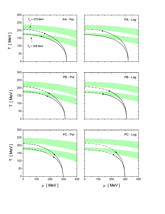
Figure 8: (Color online) Phase diagrams for parametrizations PA ( top), PB (center) and PC ( bottom), considering polynomial (left) and logarithmic (right) PL potentials, with both $T_{0}=270$ and 208 MeV. Solid lines correspond to first order chiral transitions, while dashed (dotted) lines correspond to chiral (deconfinement) crossover-like transitions. Dash-dotted lines stand for the cases in which both crossover-like transitions coincide. The green bands indicate the regions in which $0.3\leq\Phi\leq 0.5$.

The phase diagrams corresponding to the three nonlocal NJL model parameterizations introduced in Sec. 2.3 are displayed in Fig. 8. Upper, central and lower panels show the results for PA, PB and PC, respectively, while left (right) panels correspond to the polynomial (logarithmic) potentials. In each panel, both the diagrams associated to $T_{0}=270$ MeV and $T_{0}=208$ MeV are shown. Solid and dashed lines indicate the critical temperatures for first order and crossover-like chiral restoration transitions, dotted lines correspond to the peaks of the PL susceptibility, and the green bands indicate the regions in which $0.3\leq\Phi\leq 0.5$. It is observed that, as in the $\mu=0$ case, the deconfinement and chiral restoration transitions occur at basically the same critical temperature in the whole range of values of $\mu$ for which the chiral transition is crossover-like. In fact, for the logarithmic potential both transitions overlap, which is indicated by the dash-dotted lines in the right panels of Fig. 8. For the polynomial potential, the splitting between the critical temperatures $T_{\rm ch}$ and $T_{\Phi}$ does not exceed the values obtained for $\mu=0$, namely $|T_{\rm ch}-T_{\Phi}|\lesssim 6$ MeV. In principle, the dotted lines (peaks of the PL susceptibility) could also be extended to $\mu>\mu_{\rm CEP}$; at $\mu=\mu_{\rm CEP}$ they are found to suffer a discontinuity, after which they fall within the green bands. These lines are not shown in Fig. 8 since, as stated, in that region we find it preferable to define the deconfinement transition temperatures through the bands where $\Phi$ lies in the range from 0.3 to 0.5.

Concerning the character of the transitions, it is seen that the case of PA and a logarithmic PL potential, with $T_{0}=208$ MeV, is the only one for which the transition is always of first order. For all other parametrizations and PL potentials, there is a CEP at which the chiral transition changes its character from crossover to first order as $\mu$ grows. Once the transition becomes of first order (i.e. for $\mu>\mu_{\rm CEP}$) the critical temperatures for chiral restoration start to decrease quite fast as $\mu$ increases, reaching the $T=0$ axis at a certain value value $\mu_{c}(0)$. Beyond that critical chemical potential, the system lies in a phase where chiral symmetry is approximately restored for all values of $T$. However, as mentioned above, for temperatures below the green bands quarks are still confined and in these regions the system is in the quarkyonic phase. Similar phase transition features have been found within other effective approaches for low energy QCD, as e.g. the quark-meson and Polyakov-quark-meson models, both at the mean field level Schaefer:2007pw and after the inclusion of meson fluctuations Herbst:2010rf ; Herbst:2013ail ; Pawlowski:2014zaa . For those models it is seen that the inclusion of beyond mean field corrections can affect significantly the location of the CEP in the $\mu-T$ plane.

The position of the most relevant points in the phase diagrams are quoted in Table 3. Given a value of $T_{0}$, the main difference between parametrizations PA, PB and PC resides in the location of the CEP. In general, parametrization PA —which does not account for WFR effects— leads to lower values of $\mu_{\rm CEP}$. Comparing the results of PB and PC we observe that the latter leads to somewhat lower values of $T_{\rm CEP}$ and higher values of $\mu_{\rm CEP}$. The position of the critical end point is also quite sensitive to the amount of explicit breakdown of chiral symmetry (i.e., the size of current quark masses). This is illustrated in Fig. 9, where we plot the values of $T_{\rm CEP}$ (left panel) and $\mu_{\rm CEP}$ (right panel) as functions of the ratio $m_{\pi}/m_{\pi}^{\rm phys}$. The results correspond to the logarithmic PL potential, with $T_{0}=208$ MeV. As discussed in Sec. 2.4, the values of $m_{\pi}$ are obtained by varying the value of the current quark mass $m_{c}$ while keeping fixed other model parameters. Note that for a pion mass $m_{\pi}\sim 1.75\,m_{\pi}^{\rm phys}$ a second CEP appears at low chemical potentials. This is due to the fact that the phase transition at $\mu=0$ becomes of first order, and consequently a crossover line connects the two CEPs. As $m_{\pi}$ increases this crossover line gets shortened, until at $m_{\pi}/m_{\pi}^{\rm phys}\sim 2$ the two CEPs meet. Beyond that value the whole transition line becomes of first order. Although it is likely that the predicted values for these critical pion masses are too low, it would be interesting to verify if this behavior of the CEP position as a function of the amount of explicit symmetry breaking is supported by other model calculations.

	$T_{0}=208$
	PA			PB			PC
	Pol	Log		Pol	Log		Pol	Log
$T_{\chi}(0)$	178	174		178	171		181	173
$T_{\Phi}(0)$	175	174		174	171		175	173
$\mu_{\rm CEP}$	135	$-$		180	135		227	213
$T_{\rm CEP}$	162	$-$		147	162		125	141
$\mu_{c}(0)$	322	322		312	312		298	298
	$T_{0}=270$
	PA			PB			PC
	Pol	Log		Pol	Log		Pol	Log
$T_{\chi}(0)$	210	210		210	210		214	215
$T_{\Phi}(0)$	206	210		206	210		210	215
$\mu_{\rm CEP}$	160	132		193	182		232	235
$T_{\rm CEP}$	181	198		165	182		142	154
$\mu_{c}(0)$	322	322		312	312		298	298

Table 3: Positions of some characteristic points in the $\mu-T$ phase diagram for various nlPNJL model parametrizations. All values are given in MeV.

Figure 9: (Color online) CEP temperature and chemical potential as functions of the pion mass. The results correspond to the logarithmic PL potential, with $T_{0}=208$ MeV.

2.6 Extension to imaginary chemical potential

In this section we address the extension of previous analyses to the case of imaginary chemical potential. As mentioned above, this deserves significant theoretical interest, since for imaginary $\mu$ lattice QCD calculations do not suffer from the sign problem Alford:1998sd ; D'Elia:2002gd ; deForcrand:2002hgr ; Wu:2006su , and the corresponding results can be compared with the predictions arising from effective models. It is seen that lattice data, as well as analyses based on the exact renormalization group equations Braun:2009gm , suggest a close relation between the deconfinement and chiral restoration transitions for imaginary chemical potentials. In addition, the behavior of physical quantities in the region of imaginary chemical potential is expected to have implications on the QCD phase diagram at finite real values of $\mu$ Karbstein:2006er ; Bonati:2015bha ; Bellwied:2015rza ; Borsanyi:2020fev .

As shown by Roberge and Weiss (RW) Roberge:1986mm , the QCD thermodynamic potential in the presence of an imaginary chemical potential $\mu=i\theta T$ is invariant under the so-called extended $Z_{3}$ symmetry transformations, which are given by a combination of a $Z_{3}$ transformation of the quark and gauge fields and a shift $\theta\rightarrow\theta+2k\pi/3$. The RW symmetry is a remnant of the $Z_{3}$ symmetry that exists in the pure gauge theory. In QCD with dynamical quarks, if the temperature is larger than a certain value $T_{RW}$ it can be seen that three $Z_{3}$ vacua appear. They can be classified according to the corresponding Polyakov loop phases, viz. $\varphi$, $\varphi+2\pi/3$ and $\varphi+4\pi/3$. It should be stressed that, as mentioned in Sec. 2.2, for imaginary chemical potential the restriction of having $\Phi\,\in\,\mathbb{R}$ in order to get a real thermodynamic potential is lost. Thus, both $\phi_{3}$ and $\phi_{8}$ can be nonvanishing. For $T>T_{RW}$ there is a first order phase transition at $\theta=\pi/3$ mod $2\pi/3$ —known as the “Roberge-Weiss transition”— in which the vacuum jumps to one of its $Z_{3}$ images. The point at the end of the RW transition line in the $(T,\theta)$ plane, i.e. $(T,\theta)=(T_{RW},\pi/3)$, is known as the “RW end point”. The order of the RW transition at the RW end point has been subject of considerable interest in the last years in the framework of lattice QCD D'Elia:2007ke ; D'Elia:2009qz ; deForcrand:2010he ; Bonati:2010gi ; Bonati:2018fvg ; Goswami:2018qhc , due to the implications it might have on the QCD phase diagram at finite real chemical potential. According to $N_{f}=2$ LQCD calculations, it appears that the RW end point is first order for realistically small values of the current quark mass.

It is not difficult to show that the RW symmetry is also present in nlPNJL models Pagura:2011rt ; Kashiwa:2011td . This can be done as follows. The last two terms of the thermodynamic potential in the r.h.s. of Eq. (40) are clearly invariant under the transformations

$$\Phi(\theta)\ \rightarrow\ \Phi(\theta)\exp(-i\,2\,k\,\pi/3)\ ,\qquad\qquad\theta\ \rightarrow\ \theta+2\,k\,\pi/3\ .$$ (56)

To check the invariance of the first term, notice that the first of the transformations in Eq. (56) can be obtained through

$$\phi_{3}(\theta)\ \rightarrow\ \phi_{3}(\theta)\ ,\qquad\qquad\phi_{8}(\theta)\ \rightarrow\ \phi_{8}(\theta)-2\,k\,\pi\,T/\sqrt{3}\ .$$ (57)

Taking into account Eqs. (56) and (57), from the definition of $(\rho_{n,\vec{p}}^{c})^{2}$ in Eq. (40) it is easy to see that any sum of the form $\sum_{c=r,g,b}F[(\rho_{n,\vec{p}}^{c})^{2}]$, where $F$ is an arbitrary function, is invariant under the extended $Z_{3}$ symmetry transformations. The invariance of the terms introduced through the regularization of the thermodynamic potential can be shown in a similar way. As a further evidence of the $Z_{3}$ invariance of the model, it is interesting to study the behavior of the order parameters as functions of $T$ and $\theta$. For this analysis it is useful to introduce an “extended traced Polyakov loop” $\Psi$, defined by $\Psi=\exp(i\theta)\Phi$. The latter is invariant by construction under the transformations in Eq. (56), and its phase $\psi$ can be taken as order parameter of the RW transition Sakai:2008um .

In what follows we discuss some of the results obtained using the nlPNJL model parametrizations introduced in Sec. 2.3 Pagura:2011rt ; Pagura:2013rza . Similar results arising from some alternative parametrization have been quoted in Ref. Kashiwa:2011td , while results from the Polyakov-quark-meson model, including meson fluctuations, can be found in Ref. Morita:2011jva . First, let us keep $T$ constant and verify the periodicity of thermodynamic quantities as functions of $\theta$. For definiteness we concentrate for now in the case of the logarithmic potential. In Fig. 10 we display, from above to below, the modulus of the extended PL, the phase $\psi$, the mean field value of the $\sigma_{1}$ field, the chiral condensate and the thermodynamic potential, as functions of $\theta/(\pi/3)$ for various values of $T$. The curves correspond to parametrization PB, for $T_{0}=208$ MeV. Qualitatively similar results are obtained for PC with $T_{0}=208$ MeV, as well as for all three parametrizations PA, PB and PC with $T_{0}=270$ MeV. In the case of PA with $T_{0}=208$ MeV, although the same periodicity is observed, all curves turn out to be discontinuous for temperatures in the transition region. For $T>T_{RW}$ one finds the above mentioned RW first order phase transition at $\theta=\pi/3$, which is signalled by a discontinuity in the phase $\psi$ of the extended Polyakov loop.

Figure 10: (Color online) Results for some relevant quantities as functions of $\theta/(\pi/3)$, for fixed values of the temperature. The observed periodicity is due to the fact that the nlPNJL model is invariant under the extended $Z_{3}$ symmetry transformations. The results correspond to PB and a logarithmic PL potential, with $T_{0}=208$ MeV.

On the other hand, by looking at the behavior of the order parameters and susceptibilities as functions of the temperature one can find signals of both deconfinement and chiral symmetry restoration transitions. This is clearly seen in Fig. 11, where we show the curves for the normalized quark condensate, the traced PL and the corresponding susceptibilities $\chi_{\rm ch}$ and $\chi_{\Phi}$ as functions of $T$, taking $\theta$ fixed at the representative values $\theta=\pi/6$ and $\pi/3$. The results correspond once again to parametrization PB with $T_{0}=208$ MeV. For $\theta=\pi/6$, both the deconfinement and chiral restoration transitions are found to be crossover-like. Moreover, it can be seen that the susceptibilities associated to both order parameters show peaks at a common temperature. This can be interpreted as a signal indicating an entanglement between the transitions. However, notice that $\chi_{\rm ch}$ shows at a larger temperature an additional, broader peak. For $\theta=\pi/3$, one observes at $T\simeq 190$ MeV a jump in $\Phi$ that can be understood as a first order deconfinement phase transition. However, in the case of the chiral condensate the corresponding gap is relatively small and, moreover, beyond this discontinuity one still finds the broad peak in $\chi_{\rm ch}$. Consequently, we find it reasonable to identify the chiral restoration temperature through the maximum of this broad peak. We conclude that for $\theta=\pi/3$ only the deconfinement transition is of first order, while the chiral restoration still proceeds as a crossover. For PC with $T=208$ MeV and for all three parametrizations with $T_{0}=270$ MeV the situation is very similar, whereas for PA with $T_{0}=208$ MeV the transition is of first order for any value of $\theta$ in the considered range of temperatures.

Figure 11: (Color online) Order parameters for the deconfinement and chiral restoration transitions (upper panel) and associated susceptibilities (lower panel) as functions of $T$, for $\theta=\pi/6$ and $\theta=\pi/3$. The results correspond to parametrization PB, with $T_{0}=208$ MeV.

In Fig. 12 we quote the critical temperatures as functions of $\theta$ (normalized to $\pi/3$) for parametrizations PA, PB and PC Pagura:2011rt . The results correspond to the logarithmic PL potential, with $T_{0}=208$ MeV. For comparison, values obtained from LQCD calculations taken from Ref. Wu:2006su are also shown. They have an error of about $10\%$ due the uncertainty in the determination of $T_{\rm ch}(\theta=0)$. From the figure it is seen that the predictions of the nlPNJL model for the deconfinement critical temperatures are compatible with LQCD data. Moreover, the values of $T_{RW}$ obtained within the model are found to be 191, 188 and 191 MeV for PA, PB and PC, respectively, in good agreement with the value $T_{RW}=185(9)$ MeV arising from $N_{f}=2$ LQCD calculations Wu:2006su (for $N_{f}=2+1$, LQCD results seem to favor a slightly larger value Bonati:2016pwz ).

It is also seen that there is a splitting between chiral restoration and deconfinement critical temperatures, which gets larger when $\theta$ increases. As already mentioned, there is a critical value $\theta_{\rm CEP}\sim 0.7\times\pi/3$ above which the deconfinement transition is of first order for all three parametrizations. Therefore, it is found that in all cases the transition lines are of first order when they reach the RW end point. This implies that the RW end point is a triple point, and the RW transition is also of first order there. This can be clearly seen in Fig. 13, which shows the behavior of the phase $\psi$ as a function of $T$, for $\theta=\pi/3$.

Figure 12: Critical temperatures as functions of $\theta$ for parametrizations PA, PB and PC. First order transitions are indicated with solid lines, while dotted and dashed lines correspond to deconfinement and chiral restoration transitions, respectively, in the regions where they are crossover-like. Vertical solid lines indicate the first order RW transition. The fat dots correspond to lattice QCD results

Figure 13: Phase of the extended PL loop $\Psi=\exp(i\theta)\Phi$ as a function of $T$ for $\theta=\pi/3$. The results correspond to parametrization PC and the logarithmic PL potential, with $T_{0}=208$ MeV.

Up to now we have discussed the results obtained considering a logarithmic PL potential. For the polynomial potential, the main novel qualitative feature is that there is no first order deconfinement transition. As a consequence, for this PL potential the RW transition at the end point is of second order for all considered parametrizations. This appears to be in contradiction with LQCD results reported in Refs. D'Elia:2007ke ; D'Elia:2009qz ; deForcrand:2010he ; Bonati:2010gi , which indicate that such a transition is of first order for a physical pion mass. Concerning the predictions for $T_{RW}/T_{\rm ch}(\theta=0)$, they are somewhat larger than those found for the logarithmic PL potential. On the other hand, the ratios $T_{\rm ch}(\theta=\pi/3)/T_{\rm ch}(\theta=0)$ for $T_{0}=208$ MeV ($T_{0}=270$ MeV) are similar (larger) to those obtained using the logarithmic potential.

2.7 Meson properties at finite temperature

To conclude this section, in this last subsection we concentrate on the thermal behavior of some $\sigma$ and $\pi$ meson properties. In the context of nlPNJL models, the relevant theoretical expressions can be obtained from those given in Sec. 2.1 using the Matsubara formalism, as described in Sec. 2.2. In this way, the finite temperature extension of the quadratic term in the Euclidean action [see Eq. (13)] reads

$$S_{E}^{\mathrm{quad}}\ =\ \frac{1}{2}\sum_{M=\sigma,\sigma^{\prime},\pi}\ \int_{q,m}G_{M}(\vec{q}^{\,2},\nu_{m}^{2})\;\delta M(q_{m})\,\delta M(-q_{m})\ ,$$ (58)

where $q_{m}=(\vec{q},\nu_{m})$, with $\nu_{m}=2\pi mT$. Here the notation

$$\int_{q,m}\ \equiv\ T\sum_{m=-\infty}^{\infty}\int\frac{d^{3}q}{(2\pi)^{3}}$$ (59)

has been used. For charged and neutral pions one has

$$G_{\pi}(\vec{q}^{\,2},\nu_{m}^{2}) = \frac{1}{G_{S}}-8\sum_{c}\int_{p,n}g\Big{(}p_{nc}+\frac{q_{m}}{2}\Big{)}^{2}\ \frac{Z(p_{nc}+q_{m})Z(p_{nc})}{D(p_{nc}+q_{m})D(p_{nc})}$$ (60)

$$\times\left[p_{nc}^{2}+p_{nc}\cdot q_{m}+M(p_{nc}+q_{m})M(p_{nc})\right]\ ,$$

where $p_{nc}=(\vec{p},(2n+1)\pi T-\phi_{c})$ and $D(p)=p^{2}+M(p)^{2}$. In the case of the $\sigma$ and $\sigma^{\prime}$ mesons, the $G_{M}$ functions are given by

$$G_{{\sigma\choose{\sigma^{\prime}}}}(\vec{q}^{\,2},\nu_{m}^{2}) = \frac{G_{\sigma_{1}\sigma_{1}}(\vec{q}^{\,2},\nu_{m}^{2})+G_{\sigma_{2}\sigma_{2}}(\vec{q}^{\,2},\nu_{m}^{2})}{2}$$ (61)

$$\mp\,\sqrt{\left[G_{\sigma_{1}\sigma_{2}}(\vec{q}^{\,2},\nu_{m}^{2})\right]^{2}+\left[\frac{G_{\sigma_{1}\sigma_{1}}(\vec{q}^{\,2},\nu_{m}^{2})-G_{\sigma_{2}\sigma_{2}}(\vec{q}^{\,2},\nu_{m}^{2})}{2}\right]^{2}}\ ,$$

where

$$G_{\sigma_{1}\sigma_{1}}(\vec{q}^{\,2},\nu_{m}^{2}) = \frac{1}{G_{S}}-8\sum_{c}\int_{p,n}\,g\left(p_{nc}+\frac{q_{m}}{2}\right)^{2}\frac{Z(p_{nc}+q_{m})Z(p_{nc})}{D(p_{nc}+q_{m})D(p_{nc})}$$

$$\times\left[p_{nc}^{2}+p_{nc}\cdot q_{m}-M(p_{nc}+q_{m})M(p_{nc})\right],$$

$$G_{\sigma_{2}\sigma_{2}}(\vec{q}^{\,2},\nu_{m}^{2}) = \frac{1}{G_{S}}+\frac{8}{\varkappa_{p}^{2}}\sum_{c}\int_{p,n}\,\left(p_{nc}+\frac{q_{m}}{2}\right)^{2}\,f\left(p_{nc}+\frac{q_{m}}{2}\right)^{2}\frac{Z(p_{nc}+q_{m})Z(p_{nc})}{D(p_{nc}+q_{m})D(p_{nc})}$$

$$\times\left[p_{nc}^{2}+p_{nc}\cdot q_{m}-M(p_{nc}+q_{m})M(p_{nc})+\frac{p^{2}_{nc}(p_{nc}+q_{m})^{2}-(p^{2}_{nc}+p_{nc}\cdot q_{m})^{2}}{2(p_{nc}+q_{m}/2)^{2}}\right]\ ,$$

$$G_{\sigma_{1}\sigma_{2}}(\vec{q}^{\,2},\nu_{m}^{2}) = -\frac{8}{\varkappa_{p}^{2}}\sum_{c}\int_{p,n}\,g\left(p_{nc}+\frac{q_{m}}{2}\right)f\left(p_{nc}+\frac{q_{m}}{2}\right)\frac{Z(p_{nc}+q_{m})Z(p_{nc})}{D(p_{nc}+q_{m})D(p_{nc})}$$ (62)

$$\times\left(p_{nc}+\frac{q_{m}}{2}\right)\cdot\left[p_{nc}\,M(p_{nc}+q_{m})+(p_{nc}+q_{m})M(p_{nc})\right]\ .$$

As in the $T=0$ case discussed in Sec. 2.1, the meson masses can be found by looking for the poles of the corresponding propagators. In the present case they are given by the solutions of the equations

$$G_{M}(-m_{M}^{2},0)\ =\ 0\ .$$ (63)

The masses obtained in this way correspond to the spatial screening masses associated with Matsubara zero modes. They determine a behavior $\sim\exp(-m_{M}\,r)$ in configuration space, i.e., the reciprocals $m_{M}^{-1}$ describe the persistence lengths of zero modes in equilibrium with the thermal bath. In fact, these masses are the quantities that are usually studied in LQCD calculations Karsch:2003jg . It should be noted that one has a screening mass for each Matsubara mode.

Another relevant physical quantity to be studied is the pion decay constant $f_{\pi}$. Its finite temperature behavior provides another way to characterize the chiral restoration transition. To obtain the corresponding expression at finite temperature we replace $F_{0}$ in Eq. (27) by

$$F_{0}(\vec{q}^{\,2},\nu_{m}^{2}) = 8\sum_{c}\int_{p,n}{g\left(p_{nc}+\frac{q_{m}}{2}\right)}\frac{Z(p_{nc}+q_{m})Z(p_{nc})}{D(p_{nc}+q_{m})D(p_{nc})}$$ (64)

$$\times\ \left[p_{nc}^{2}+p_{nc}\cdot q_{m}+M(p_{nc}+q_{m})M(p_{nc})\right]\ ,$$

to be evaluated at $(\vec{q}^{\,2},\nu_{m}^{2})=(-m_{\pi}^{2},0)$.

Figure 14: (Color online) Masses of $\sigma$ and $\pi$ mesons as functions of $T/T_{\rm ch}$ for polynomial (left) and logarithmic (right) PL potentials, with $T_{0}=208$ MeV. In each panel the results for parametrizations PA, PB and PC are shown.

Let us analyze the numerical results obtained for the above meson properties in the context of nlPNJL models. We start by discussing the behavior of $\sigma$ and $\pi$ meson masses. As mentioned in Sec. 2.3, at $T=0$ one gets $m_{\sigma}=683$, 622 and 554 MeV for parametrizations PA, PB and PC, respectively, while the value $m_{\pi}(T=0)=139$ MeV has been taken in all cases as one of the inputs for the determination of the model parameters. In Fig. 14 we show the behavior of $\sigma$ and $\pi$ masses as functions of $T/T_{\rm ch}$, for polynomial (left) and logarithmic (right) PL potentials, taking $T_{0}=208$ MeV. In each panel the curves corresponding to PA, PB and PC are displayed. Starting from $T=0$, it is seen that if the temperature is increased the masses remain almost constant up approximately the chiral restoration critical temperature. Close to that temperature the $\sigma$ mass shows a sudden drop and the $\pi$ mass starts to increase, and both curves meet at $T\gtrsim T_{\rm ch}$. Then the masses of both chiral partners grow together towards their asymptotic value $2\pi T$, associated with an uncorrelated $q\bar{q}$ pair Florkowski:1993br ; Eletsky:1988an . By analyzing the curves in more detail it can be seen that for the largest temperature considered in the graph such a limit has not been reached yet. This is due to the fact that for $T/T_{\rm ch}\sim 1.4$ the contribution of the PL parameter $\phi_{3}$ to the quark screening masses still is nonnegligible. In fact, after the restoration of chiral symmetry the curves in the figure grow according to $m_{M}=2(\pi T-\phi_{3})$, behaving as straight lines with approximately the same slope. Finally, it should be noted that in the right panel (corresponding to the logarithmic potential) there is a discontinuity in the masses for parametrization PA. This is associated with the fact that the chiral restoration transition is of first order in that case. Except for this particularity, the thermal behavior of the $\sigma$ and $\pi$ masses is qualitatively similar in all considered cases. Results for $T_{0}=270$ MeV, which also include medium induced Lorentz braking effects, can be found in Ref. Benic:2013eqa . They turn out to be very similar to those shown in Fig. 14.

Finally, in Fig. 15 we show the temperature dependence of the pion decay constant $f_{\pi}$, for the three parametrizations under consideration. Left and right panels correspond to polynomial and logarithmic PL potentials, respectively. It is found that, again, the only case that presents a distinct behavior is that of PA with the logarithmic PL potential, where the curves show a discontinuity at the transition temperature.

Figure 15: (Color online) Pion decay constant $f_{\pi}$ as a function of $T/T_{\rm ch}$ for polynomial (left) and logarithmic (right) PL potentials, with $T_{0}=208$ MeV. In each panel the results for parametrizations PA, PB and PC are shown.

3 Two-flavor nonlocal NJL model including vector and axial vector quark currents

In this section we study an extension of the previously considered nlNJL models in which vector and axial vector quark current-current interactions are included. This allows for a description of vector and axial vector meson phenomenology. The cases of both zero and finite temperature and/or quark chemical potential are discussed.

3.1 Formalism at vanishing temperature and chemical potential

3.1.1 Effective action and mean field equations

As stated, in what follows we analyze a two-flavor nlNJL chiral quark model that includes nonlocal vector and axial vector quark-antiquark currents. This type of model has been studied e.g. in Refs. Villafane:2016ukb ; Contrera:2012wj ; Contrera:2016rqj ; Carlomagno:2019yvi . We consider an effective Euclidean action given by Villafane:2016ukb

$$S_{E} = \int d^{4}x\ \left\{\bar{\psi}(x)(-\,i\not{\partial}+m_{c})\psi(x)-\frac{G_{S}}{2}\Big{[}j_{S}(x)j_{S}(x)+\vec{\jmath}_{P}(x)\cdot\vec{\jmath}_{P}(x)+j_{R}(x)j_{R}(x)\Big{]}\right.$$ (65)

$$\left.-\,\frac{G_{V}}{2}\Big{[}\vec{\jmath}_{V\mu}(x)\cdot\vec{\jmath}_{V\mu}(x)+\vec{\jmath}_{A\,\mu}(x)\cdot\vec{\jmath}_{A\,\mu}(x)\Big{]}-\frac{G_{0}}{2}\;j^{\,0}_{V\mu}(x)\,j^{\,0}_{V\mu}(x)-\frac{G_{5}}{2}\;j^{\,0}_{A\,\mu}(x)\,j^{\,0}_{A\,\mu}(x)\right\}\ .$$

As in Sec. 2 we work in the isospin limit; thus, we assume the current mass to be the same for $u$ and $d$ quarks. The model includes the four-fermion couplings studied in Sec. 2.1.1 [see Eqs. (1) and (2)], plus additional vector and axial vector pieces. The new quark-antiquark currents read

$$\vec{\jmath}_{V\mu}(x) = \int d^{4}z\;{\cal H}(z)\,\bar{\psi}\left(x+\frac{z}{2}\right)\vec{\tau}\gamma_{\mu}\psi\left(x-\frac{z}{2}\right)\ ,$$

$$\vec{\jmath}_{A\,\mu}(x) = \int d^{4}z\;{\cal H}(z)\,\bar{\psi}\left(x+\frac{z}{2}\right)\vec{\tau}\gamma_{\mu}\gamma_{5}\psi\left(x-\frac{z}{2}\right)\ ,$$

$$j^{\,0}_{V\mu}(x) = \int d^{4}z\;{\cal H}_{0}(z)\,\bar{\psi}\left(x+\frac{z}{2}\right)\gamma_{\mu}\psi\left(x-\frac{z}{2}\right)\ ,$$

$$j^{\,0}_{A\,\mu}(x) = \int d^{4}z\;{\cal H}_{5}(z)\,\bar{\psi}\left(x+\frac{z}{2}\right)\gamma_{\mu}\gamma_{5}\psi\left(x-\frac{z}{2}\right)\ ,$$ (66)

where the functions ${\cal H}(z)$, ${\cal H}_{0}(z)$ and ${\cal H}_{5}(z)$ are covariant nonlocal form factors. Notice that, in order to guarantee chiral invariance, the couplings involving the currents $\vec{\jmath}_{V\mu}$ and $\vec{\jmath}_{A\,\mu}$ have to carry the same form factor ${\cal H}(z)$.

As discussed in Sec. 2.1.1, for the study of meson phenomenology it is convenient to perform a bosonization of the fermionic theory. In the present case, this is done by introducing the auxiliary bosonic fields $\sigma_{1}(x)$, $\sigma_{2}(x)$ and $\pi_{a}(x)$ previously considered in Sec. 2, as well as new fields $v^{0}_{\mu}(x)$, $v^{a}_{\mu}(x)$ (vector) and $a^{0}_{\mu}(x)$, $a^{a}_{\mu}(x)$ (axial vector), where indices $a$ run from 1 to 3. After integrating out the fermion fields the partition function can be written as

$$\mathcal{Z} = \int{\rm D}\sigma_{1}\,{\rm D}\sigma_{2}\,{\rm D}\,\vec{\pi}\,{\rm D}\,v^{0}_{\mu}\,{\rm D}\,a^{0}_{\mu}\,{\rm D}\,\vec{v}_{\mu}\,{\rm D}\,\vec{a}_{\mu}\;\exp\big{(}\!-S_{E}^{\rm bos}\big{)}\ ,$$ (67)

where $S_{E}^{\rm bos}$ stands for the Euclidean bosonized action. In momentum space, the latter is given by

$$S^{\rm bos}_{E} = -\ln\,\det{\cal D}+\int\dfrac{d^{4}q}{(2\pi)^{4}}\left\{\dfrac{1}{2G_{S}}\left[\sigma_{1}(q)\sigma_{1}(-q)+\vec{\pi}(q)\cdot\vec{\pi}(-q)+\sigma_{2}(q)\sigma_{2}(-q)\right]\right.$$ (68)

$$+\left.\dfrac{1}{2G_{V}}\left[\vec{v}_{\mu}(q)\cdot\vec{v}_{\mu}(-q)+\vec{a}_{\mu}(q)\cdot\vec{a}_{\mu}(-q)\right]+\dfrac{1}{2G_{0}}\;v^{0}_{\mu}(q)v^{0}_{\mu}(-q)+\dfrac{1}{2G_{5}}\;a^{0}_{\mu}(q)a^{0}_{\mu}(-q)\right\}\ ,$$

where the operator ${\cal D}(p,p^{\prime})$ reads

$${\cal D}(p,p^{\prime}) = (2\pi)^{4}\delta^{(4)}(p-p^{\prime})(\hbox to0.0pt{/\hss}p+m_{c})+g(\bar{p})\,\bigg{[}\sigma_{1}(p-p^{\prime})+i\gamma_{5}\vec{\tau}\cdot\vec{\pi}(p-p^{\prime})\bigg{]}$$ (69)

$$-\ f(\bar{p})\,\dfrac{\hbox to0.0pt{/\hss}\bar{p}}{\varkappa_{p}}\,\sigma_{2}(p-p^{\prime})\ +\ h(\bar{p})\,\gamma_{\mu}\bigg{[}\vec{\tau}\cdot\vec{v}_{\mu}(p-p^{\prime})+\gamma_{5}\,\vec{\tau}\cdot\vec{a}_{\mu}(p-p^{\prime})\bigg{]}$$

$$+\ h_{0}(\bar{p})\,\gamma_{\mu}\;v^{0}_{\mu}(p-p^{\prime})+\ h_{5}(\bar{p})\,\gamma_{\mu}\gamma_{5}\;a^{0}_{\mu}(p-p^{\prime})\ ,$$

with $\bar{p}\equiv(p+p^{\prime})/2$. The functions $f(p)$, $g(p)$, $h(p)$, $h_{0}(p)$, and $h_{5}(p)$ stand for the Fourier transforms of the form factors entering the nonlocal currents. Without loss of generality, the coupling constants can be chosen in such a way that the form factors are normalized to $f(0)=g(0)=h(0)=h_{0}(0)=h_{5}(0)=1$. Next, the bosonic fields can be expanded around their vacuum expectation values, $\phi(x)=\bar{\phi}+\delta\phi(x)$. As done in Sec. 2.1.1, on the basis of charge, parity and Lorentz symmetries, it is assumed that in vacuum only $\sigma_{1}(x)$ and $\sigma_{2}(x)$ have nontrivial translational invariant mean field values. These are denoted by $\bar{\sigma}_{1}$ and $\varkappa_{p}\,\bar{\sigma}_{2}$, respectively, while vacuum expectation values of the remaining bosonic fields are taken to be zero. Notice that, as discussed below, at nonvanishing chemical potential Lorentz symmetry is broken, and the mean field expectation value of $v_{4}^{0}(x)$ can also be nonzero. Following similar steps as those described in Sec. 2.1.1, the bosonized effective action in Eq. (68) can be expanded in powers of meson fluctuations as

$$S_{E}^{\rm bos}\ =\ S_{E}^{\rm MFA}\;+\;S_{E}^{\rm quad}\;+\;\dots\$$ (70)

It turns out that the mean field piece $S_{E}^{\rm MFA}$ is the same as the one given in Eq. (10). Therefore, the corresponding gap equations coincide with Eqs. (18) and (19). As found in Sec. 2.1.1, the mean field quark propagator is given by

$$\mathcal{S}_{0}(p)\ =\mathcal{D}_{0}(p)^{-1}\ =\ \frac{Z(p)}{\hbox to0.0pt{/\hss}p+M(p)}\ ,$$ (71)

with

$$Z(p)=\left(1-\bar{\sigma}_{2}\ f(p)\right)^{-1}\ ,\qquad\qquad M(p)=Z(p)\left(m_{c}+\bar{\sigma}_{1}\ g(p)\right)\ .$$ (72)

3.1.2 Meson masses and decay constants

In this subsection we discuss the analytical expressions to be used for the calculation of basic meson phenomenological quantities, such as masses and decay constants. It is important to notice that pion observables, already calculated within the nonlocal NJL approach in Sec. 2.1.3, need to be revisited owing to the mixing between pion and axial vector fields.

As discussed in Sec. 2.1.3, the meson masses can be obtained from the piece of the Euclidean action that is quadratic in the bosonic fields, $S_{E}^{\rm quad}$. In the present case one has

$$S_{E}^{\rm quad} = \dfrac{1}{2}\int\frac{d^{4}q}{(2\pi)^{4}}\ \Big{\{}G_{\sigma}(q^{2})\,\delta\sigma(q)\,\delta\sigma(-q)+G_{\sigma^{\prime}}(q^{2})\,\delta\sigma^{\prime}(q)\,\delta\sigma^{\prime}(-q)$$ (73)

$$+\;G_{\pi}(q^{2})\,\delta\vec{\pi}(q)\cdot\delta\vec{\pi}(-q)-i\,G_{\pi a}(q^{2})\Big{[}q_{\mu}\,\delta\vec{a}_{\mu}(-q)\cdot\delta\vec{\pi}(q)-q_{\mu}\,\delta\vec{a}_{\mu}(q)\cdot\delta\vec{\pi}(-q)\Big{]}$$

$$+\;G_{0\,\mu\nu}(q^{2})\,\delta v^{0}_{\mu}(q)\,\delta v^{0}_{\nu}(-q)+G_{5\,\mu\nu}(q^{2})\,\delta a^{0}_{\mu}(q)\,\delta a^{0}_{\nu}(-q)$$

$$+\;G_{v\,\mu\nu}(q^{2})\,\delta\vec{v}_{\mu}(q)\cdot\delta\vec{v}_{\nu}(-q)+G_{a\,\mu\nu}(q^{2})\,\delta\vec{a}_{\mu}(q)\cdot\delta\vec{a}_{\nu}(-q)\Big{\}}\ ,$$

where the functions $G_{M}(q^{2})$, $M=\sigma,\sigma^{\prime},\pi,\dots$ include one-loop integrals arising from the fermionic determinant in the bosonized action. The analysis of the scalar meson sector is similar to the one discussed in Sec. 2.1.1, i.e., the mass eigenstates $\delta\sigma$ and $\delta\sigma^{\prime}$ are defined as linear combinations of $\delta\sigma_{1}$ and $\delta\sigma_{2}$ as in Eq. (14). Moreover, the expressions for $G_{\sigma}(q^{2})$ and $G_{\sigma^{\prime}}(q^{2})$ are the same as those given by Eqs. (16-17). To analyze the vector meson sector one has to take into account the tensors $G_{v\,\mu\nu}$, $G_{a\,\mu\nu}$, $G_{0\,\mu\nu}$ and $G_{5\,\mu\nu}$. From the expansion of the fermionic determinant one gets Villafane:2016ukb

$$G_{v\,\mu\nu}(q^{2}) = G_{\rho}(q^{2})\left(\delta_{\mu\nu}-\dfrac{q_{\mu}q_{\nu}}{q^{2}}\right)+L_{+}(q^{2})\dfrac{q_{\mu}q_{\nu}}{q^{2}}\ ,$$

$$G_{a\,\mu\nu}(q^{2}) = G_{{\rm a}_{1}}(q^{2})\left(\delta_{\mu\nu}-\dfrac{q_{\mu}q_{\nu}}{q^{2}}\right)+L_{-}(q^{2})\dfrac{q_{\mu}q_{\nu}}{q^{2}}\ ,$$ (74)

where

$$G_{\rho\choose{\rm a}_{1}}(q^{2}) = \dfrac{1}{G_{V}}-8N_{c}\int\dfrac{d^{4}p}{(2\pi)^{4}}\,h(p)^{2}\,\dfrac{Z(p^{+})Z(p^{-})}{D(p^{+})D(p^{-})}\,\left[\dfrac{p^{2}}{3}+\dfrac{2(p\cdot q)^{2}}{3q^{2}}-\dfrac{q^{2}}{4}\pm M(p^{-})M(p^{+})\right],$$ (75)

$$L_{\pm}(q^{2}) = \dfrac{1}{G_{V}}-8N_{c}\int\dfrac{d^{4}p}{(2\pi)^{4}}\,h(p)^{2}\,\dfrac{Z(p^{+})Z(p^{-})}{D(p^{+})D(p^{-})}\,\left[p^{2}-\dfrac{2(p\cdot q)^{2}}{q^{2}}+\dfrac{q^{2}}{4}\pm M(p^{-})M(p^{+})\right],$$ (76)

with $p^{\pm}=p\pm q/2$. The functions $G_{\rho,{\rm a}_{1}}(q^{2})$ and $L_{\pm}(q^{2})$ correspond to the transverse and longitudinal projections of the vector and axial vector fields, describing meson states with spin 1 and 0, respectively. Thus, the masses of the physical $\rho^{0}$ and $\rho^{\pm}$ vector mesons (which are degenerate in the isospin limit) can be obtained by solving the equation

$$G_{\rho}(-m_{\rho}^{2})\ =\ 0\ .$$ (77)

In addition, in order to obtain the physical states, the vector meson fields have to be normalized through

$$\delta v^{a}_{\mu}(q)\ =\ Z_{\rho}^{1/2}\;{\tilde{v}}^{a}_{\mu}(q)\ ,$$ (78)

where

$$Z_{\rho}^{-1}\ =\ g_{\rho q\bar{q}}^{-2}\ =\ \frac{dG_{\rho}(q^{2})}{dq^{2}}\bigg{|}_{q^{2}=-m_{\rho}^{2}}\ .$$ (79)

Here, $g_{\rho q\bar{q}}$ can be viewed as an effective $\rho$ meson-quark effective coupling constant. Regarding the isospin zero channels, it is easy to see that the expressions for $G_{0\,\mu\nu}(q^{2})$ can be obtained from those for $G_{v\,\mu\nu}(q^{2})$, just replacing $G_{V}\to G_{0}$ and $h(p)\to h_{0}(p)$. The $I=0$, $J^{P}=1^{-}$ state can be naturally associated with the $\omega$ vector meson, denoting by $G_{\omega}(q^{2})$ the form factor corresponding to the transverse part of $G_{0\,\mu\nu}(q^{2})$. Thus, the $\omega$ mass and wave function renormalization can be obtained as in Eqs. (78) and (79). Similar relations apply to the $I=0$ axial vector sector, where $G_{5\,\mu\nu}(q^{2})$ can be obtained from $G_{a\,\mu\nu}(q^{2})$ by replacing $G_{V}\to G_{5}$ and $h(p)\to h_{5}(p)$. The lightest physical state associated to this sector ($I=0$, $J^{P}=1^{+}$) is the $f_{1}$ axial vector meson. Hence, we denote by $G_{f_{1}}(q^{2})$ the form factor corresponding to the transverse part of $G_{5\,\mu\nu}(q^{2})$.

In the case of the pseudoscalar sector, it is seen from Eq. (73) that there is a mixing between the pion fields and the longitudinal part of the axial vector fields Ebert:1985kz ; Bernard:1993rz . The mixing term includes a loop function $G_{\pi a}(p^{2})$, while the term quadratic in $\delta\pi$ is proportional to $G_{\pi}(p^{2})$. These functions are given by

$$G_{\pi}(q^{2}) = \dfrac{1}{G_{S}}\,-\,8N_{c}\int\dfrac{d^{4}p}{(2\pi)^{4}}\;g(p)^{2}\,\dfrac{Z(p^{+})Z(p^{-})}{D(p^{+})D(p^{-})}\,\left[p^{+}\cdot p^{-}\,+\,M(p^{+})\,M(p^{-})\right]\ ,$$

$$G_{\pi a}(q^{2}) = \dfrac{8N_{C}}{q^{2}}\,\int\dfrac{d^{4}p}{(2\pi)^{4}}\,g(p)\,h(p)\,\dfrac{Z(p^{+})Z(p^{-})}{D(p^{+})D(p^{-})}\,\left[p^{+}\,M(p^{-})-p^{-}\,M(p^{+})\right]\cdot p\ ,$$ (80)

where once again we have used the definitions $p^{\pm}=p\pm q/2$. The physical states $\vec{\tilde{a}}_{\mu}$ and $\vec{\tilde{\pi}}$ can be now obtained through the relations Ebert:1985kz ; Bernard:1993rz

$$\delta\pi^{b}(q) = Z^{1/2}_{\pi}\;{\tilde{\pi}}^{b}(q)\ ,$$

$$\delta a^{b}_{\mu}(q) = Z^{1/2}_{a}\;{\tilde{a}}^{b}_{\mu}(q)\,+\,i\,\lambda(q^{2})\,q_{\mu}\,Z^{1/2}_{\pi}\;{\tilde{\pi}}^{b}(q)\ ,$$ (81)

where the mixing function $\lambda(q^{2})$, defined in such a way that the cross terms in the quadratic expansion vanish, is given by

$$\lambda(q^{2})\ =\ \dfrac{G_{\pi a}(q^{2})}{L_{-}(q^{2})}\ .$$ (82)

Thus, the pion mass can be calculated from $G_{\tilde{\pi}}(-m_{\pi}^{2})=0$, where

$$G_{\tilde{\pi}}(q^{2})\ =\ G_{\pi}(q^{2})-\,q^{2}\,\lambda(q^{2})\,G_{\pi a}(q^{2})\ ,$$ (83)

while the pion WFR is obtained from

$$Z_{\pi}^{-1}\ =\ g_{\pi q\bar{q}}^{-2}\ =\ \frac{dG_{\tilde{\pi}}(q^{2})}{dq^{2}}\bigg{|}_{q^{2}=-m_{\pi}^{2}}\ .$$ (84)

In the case of the ${\rm a}_{1}$ axial vector mesons ($I=1$ triplet), since the transverse parts of the $a_{\mu}^{b}$ fields do not mix with the pions, the corresponding mass and WFR can be calculated using relations analogous to those quoted for the vector meson sector, namely Eqs. (78) and (79), with $G_{{\rm a}_{1}}(p^{2})$ given by Eq. (75).

On the other hand, the pion weak decay constant $f_{\pi}$ can be determined following similar steps as those described in Sec. 2.1.3, now taking into account the existence of $\pi-a$ mixing. One gets in this way Villafane:2016ukb

$$f_{\pi}=\dfrac{g_{\pi q\bar{q}}}{m_{\pi}^{2}}\,m_{c}\left[F_{0}(q^{2})+\lambda(q^{2})\,F_{1}(q^{2})\right]\bigg{|}_{q^{2}=-m_{\pi}^{2}}\ ,$$ (85)

where

$$F_{0}(q^{2}) = 8N_{c}\,\int\dfrac{d^{4}p}{(2\pi)^{4}}\,g(p)\,\dfrac{Z(p^{+})Z(p^{-})}{D(p^{+})D(p^{-})}\left[p^{+}\cdot p^{-}+M(p^{+})\,M(p^{-})\right]\ ,$$

$$F_{1}(q^{2}) = 8N_{c}\,\int\dfrac{d^{4}p}{(2\pi)^{4}}\,h(p)\,\dfrac{Z(p^{+})Z(p^{-})}{D(p^{+})D(p^{-})}\;q\cdot\left[p^{+}\,M(p^{-})-p^{-}\,M(q^{+})\right]\ .$$ (86)

It is important to notice that the result for $f_{\pi}$ does not depend on the path chosen for the transport function in Eq. (26). In the absence of axial-vector meson fields, the mixing term in Eq. (85) vanishes and this expression reduces to the one given in Eq. (27).

Concerning the vector and axial vector meson sector, after some lengthy calculations one can obtain analytical expressions for other physical quantities, such as the vector and axial vector decay constants $f_{v}$ and $f_{\rm a}$ and the decay widths for the processes $\rho\to\pi\pi$ and ${\rm a}_{1}\to\rho\pi$. The corresponding results can be found in Refs. Villafane:2016ukb ; Carlomagno:2019yvi .

3.2 Extension to finite T and $\mu$ in the mean field approximation

We extend now the analysis of this model to a system at finite temperature and chemical potential. Following the prescriptions described in Sec. 2.2, the grand canonical thermodynamic potential in the mean field approximation is found to be given by Kashiwa:2011td ; Contrera:2012wj ; Contrera:2016rqj ; Carlomagno:2019yvi

$$\Omega^{\rm MFA}_{\rm reg}\ =\ \Omega^{\rm MFA}\,-\,\Omega^{\rm free}_{q}\,+\,\Omega^{\rm free}_{q,\rm reg}\,+\,\Omega_{0}\ ,$$ (87)

where

$$\Omega^{\rm MFA}\,-\,\Omega^{\rm free}_{q}\ = \ -\,4T\sum_{c=r,g,b}\ \sum_{n=-\infty}^{\infty}\int\frac{d^{3}\vec{p}}{(2\pi)^{3}}\ \ln\left[\frac{(\tilde{\rho}_{n,\vec{p}}^{c})^{2}+M(\rho_{n,\vec{p}}^{c})^{2}}{Z(\rho_{n,\vec{p}}^{c})^{2}\ [(\rho_{n,\vec{p}}^{c})^{2}+m_{c}^{2}]}\right]$$ (88)

$$\ +\,\frac{\bar{\sigma}_{1}^{2}+\varkappa_{p}^{2}\;\bar{\sigma}_{2}^{2}}{2\,G_{S}}\,-\,\frac{\bar{\omega}^{2}}{2\,G_{0}}\,+\,\mathcal{U}(\Phi,\Phi^{\ast},T)\ .$$

Here, $\bar{\omega}$ stands for the mean field value of the isoscalar field $v_{4}^{0}(x)$ (which vanishes for $\mu=0$), while the function $\mathcal{U}(\Phi,\Phi^{\ast},T)$ is an effective Polyakov loop potential that accounts for color gauge field self-interactions (see Sec. 2.2). The expression for $\Omega^{\rm free}_{q,\rm reg}$ in Eq. (87) has been given in Eq. (42), and $\Omega_{0}$ is a constant that fixes $\Omega^{\rm MFA}_{\rm reg}=0$ for $T=\mu=0$.

Notice that in Eq. (88) we have also introduced the generalized momenta $\rho_{n,\vec{p}}^{c}$ and $\tilde{\rho}_{n,\vec{p}}^{c}$. The former has been defined in the same way as in Sec. 2.2, namely

$$\Big{(}{\rho_{n,\vec{p}}^{c}}\Big{)}^{2}\ =\ {\vec{p}}\ \!^{2}+\Big{[}(2n+1)\pi T+i\mu-\phi_{c}\Big{]}^{2}\ .$$ (89)

A similar definition applies to $\tilde{\rho}_{n,\vec{p}}^{c}\,$, in which $\mu$ is replaced by a shifted chemical potential $\tilde{\mu}$ given by Contrera:2012wj

$$\tilde{\mu}\ =\ \mu-g({\rho}_{n,\vec{p}}^{c})\ Z({\rho}_{n,\vec{p}}^{c})\ \bar{\omega}\ .$$ (90)

This shift arises from the presence of the nonvanishing mean field value $\bar{\omega}$, associated to the $\omega$ vector meson.

As discussed in Sec. 2.2, the mean field values of the meson fields and the traced Polyakov loop $\Phi$ can be calculated by minimizing the regularized thermodynamic potential. In the present case, Eqs. (43) have to be supplemented by the condition

$$\frac{\partial\Omega^{\rm MFA}_{\rm reg}}{\partial\bar{\omega}}\ =\ 0\ .$$ (91)

On the other hand, the quark condensates and the susceptibilities $\chi_{\rm ch}$ and $\chi_{\Phi}$, associated with chiral restoration and deconfinement transitions, can be obtained as indicated in Sec. 2.2, see Eqs. (44-46).

3.3 Model parametrization and numerical results for zero $T$ and $\mu$

As stated in Sec. 2.3, to obtain numerical predictions for physical quantities it is necessary to specify the model parameters and nonlocal form factors. For definiteness and simplicity, we take $h(p)=h_{0}(p)=g(p)$. In fact, this can be justified from the assumption of a similar effective form for the quark currents carrying angular momenta $J=0$ and $J=1$, together with an approximate degeneracy between the vector-isovector and vector-isoscalar couplings. The axial vector-isoscalar sector can be studied separately, since it decouples from the rest of the Lagrangian. Following Ref. Villafane:2016ukb we consider $h_{5}(p)=g(p)$ just to get an estimation for the constant $G_{5}$ from phenomenology.

For the form factors $g(p)$ and $f(p)$ we consider here an exponential momentum dependence as the one given by Eq. (48), which corresponds to parametrization PB of the model studied in Sec. 2. Namely, we take

$$g(p)={\rm exp}(-p^{2}/\Lambda_{0}^{2})\ ,\qquad\qquad f(p)={\rm exp}(-p^{2}/\Lambda_{1}^{2})\ .$$ (92)

As stated, the exponential functions ensure a fast ultraviolet convergence of quark loop integrals. In any case, from the analysis in the previous section it is seen that most numerical results are qualitatively similar for different form factor functions, such as those in parametrizations PB and PC. As mentioned in Sec. 2.3, the form factors introduce two additional parameters $\Lambda_{0}$ and $\Lambda_{1}$, which act as effective momentum cutoff scales. The other six free parameters entering the action in Eq. (66) are the current quark mass $m_{c}$, the coupling constants $G_{S}$, $G_{V}$, $G_{0}$ and $G_{5}$, and the parameter $\varkappa_{p}$ in the term that includes the derivative current $j_{R}(x)$.

(a)

(b)

Figure 16: (Color online) Fit to lattice data from Ref. Parappilly:2005ei for the functions $M(p)$ and $Z(p)$. Values up to $p=3$ GeV have been considered.

As discussed in the previous section, to get a close resemblance to QCD features one can require the model to reproduce the results obtained from lattice QCD calculations for the functions $M(p)$ and $Z(p)$ that characterize the effective quark propagators. Since these functions are determined by the shape of the form factors in Eq. (92), from a fit to LQCD data it is possible to obtain a set of values for $Z(0)$ and the parameters $\Lambda_{0}$ and $\Lambda_{1}$. The analysis in Ref. Carlomagno:2019yvi , taking LQCD results from Ref. Parappilly:2005ei , leads to $Z(0)=0.75$, $\Lambda_{0}=1092$ MeV and $\Lambda_{1}=1173$ MeV. The corresponding curves for the functions $M(p)$ and $Z(p)$, together with LQCD data, are shown in Fig. 16. It can be seen that the fit is somewhat inaccurate for low momenta (where errors from LQCD calculations are larger). However, as mentioned at the end of Sec. 2.2, since volume integrals in momentum space include in general $n$ powers of momentum $p$ ($n=2$ and $n=3$ for integrals in three and four dimensions, respectively), these differences in the low-momentum behavior of the form factors are not expected to have a significant effect on the numerical results.

Given the form factor functions, it is possible to determine the remaining model parameters from some set of input phenomenological quantities. Following Ref. Carlomagno:2019yvi , we consider the case in which one takes as inputs the $\pi$ and $\rho$ meson masses and the pion weak decay constant $f_{\pi}$, together with the already mentioned value $Z(0)=0.75$. This lead to the model parameter values quoted in Table 4. Regarding the coupling constant $G_{0}$, corresponding to the isoscalar vector sector, as in Refs. Contrera:2012wj ; Carlomagno:2019yvi we leave this parameter free, using the ratio $\eta=G_{0}/G_{V}$ to tune the model. In fact, the qualitative effect of this ratio gets increased in the case of a finite chemical potential, where the mean field value $\bar{\omega}$ is in general nonzero and the isoscalar vector term can contribute significantly to the mean field thermodynamic potential. Finally, the coupling constant $G_{5}$ can be in principle determined from the $f_{1}$ meson mass. However, the observed value of this mass is well above 1 GeV, which makes the determination quite uncertain. This is discussed in Ref. Villafane:2016ukb , where $G_{5}\sim G_{V}$ is obtained.

		Value
$m_{c}$	MeV	2.26
$G_{S}\Lambda_{0}^{2}$		27.78
$G_{V}\Lambda_{0}^{2}$		23.91
$G_{5}$		$\sim G_{V}\ \;$
$\varkappa_{p}$	GeV	4.265
$\Lambda_{0}$	MeV	1092
$\Lambda_{1}$	MeV	1173

Table 4: Model parameter values.

Once the model parametrization has been established, numerical predictions for different quantities can be obtained. The results for the mean field values of scalar fields, quark condensates and quark-meson effective couplings are summarized in Table 5. In addition, in Table 6 we quote some numerical predictions for meson properties, together with the corresponding experimental estimates. In general, it is seen that the values obtained for meson masses, mixing angles and decay constants are in reasonable agreement with phenomenological expectations. As in the case of the parametrization PC considered in Sec. 2, one finds relatively low values for $m_{c}$, and a somewhat large value for the light quark condensate. On the other hand, one gets $-\langle\bar{q}q\rangle m_{c}\simeq 8.1\times 10^{-5}$ GeV⁴, which is consistent with the scale-independent result obtained from the Gell-Mann-Oakes-Renner relation in Eq. (30), viz. $-\langle\bar{q}q\rangle m_{c}=f_{\pi}^{2}m_{\pi}^{2}/2\simeq 8.3\times 10^{-5}$ GeV⁴.

		Model
$\bar{\sigma}_{1}$	MeV	648
$\bar{\sigma}_{2}$		$-0.331\$
$-\langle\bar{q}q\rangle^{1/3}$	MeV	330
$g_{\pi q\bar{q}}$		7.07
$g_{\rho q\bar{q}}$		4.16
$g_{{\rm a_{1}}q\bar{q}}$		3.74

Table 5: Numerical results for various phenomenological quantities.

		Model	Phenomenology
$m_{\pi}$	MeV	139∗	139
$m_{\sigma}$	MeV	794	400$-$550
$m_{\rho}$	MeV	775∗	775
$m_{\rm a_{1}}$	MeV	1204	$1230\pm 40$
$f_{\pi}$	MeV	92.4∗	92.4
$f_{v}$		0.173	0.200
$\Gamma_{\rho\to\pi\pi}$	MeV	121	149
$\Gamma_{{\rm a}_{1}\to\rho\pi}$	MeV	185	150$-$360

Table 6: Numerical results for various meson properties. Quantities marked with an asterisk have been taken as inputs.

It is worth pointing out that effective theories based on quark current-current interactions usually present a threshold above which the constituent quarks can be simultaneously on shell. This threshold, which depends on the model parametrization and regularization prescriptions, is typically of the order of $1$ GeV. One noticeable feature of the parametrization in Table 4 is that it leads to a threshold of about $1.25$ GeV, which turns out to be above the value obtained for the $\rm a_{1}$ meson mass. This prevents the unphysical situation of a possible decay of the $\rm a_{1}$ meson into two on-shell quarks.

3.4 Phase transitions in the $\mu-T$ plane

Through the study of the behavior of the order parameters $\langle\bar{q}q\rangle$ and $\Phi$ it is possible to determine the regions of the phase diagram in which the chiral symmetry is either broken or approximately restored, as well as those in which the system lies either in confined or deconfined states. In this subsection we identify these regions in the $\mu-T$ plane, together with the features of the existing phase transitions. The numerical results correspond to the parametrization in Sec. 3.3, considering the polynomial Polyakov loop potential in Eq. (32) and $T_{0}=208$ MeV.

In general, the situation is found to be similar to the one observed in the case of the model with no vector and axial vector quark current interactions analyzed in Sec. 2.5. The results for the phase diagram are sketched in Fig. 17, where the values $\eta=0$ and $\eta=0.5$ have been considered Carlomagno:2019yvi . At vanishing chemical potential, it is seen that the system undergoes crossover-like chiral restoration and deconfinement transitions. The corresponding critical temperatures are close to each other, viz. $T_{\rm ch}(0)=202$ MeV and $T_{\Phi}(0)=194$ MeV. They are found to be somewhat larger than those obtained for the model in Sec. 2, due to the different parametrizations considered. Now, taking a fixed temperature and increasing the chemical potential, it is seen that for $T\lesssim T_{\rm ch}(0)$ both crossover-like transitions occur at some approximately common critical value $\mu=\mu_{c}(T)$. This is shown in Fig. 17, where chiral restoration and deconfinement curves are indicated with dashed and dotted lines, respectively. Both crossover lines end at a critical end point (CEP) of coordinates $(\mu_{\rm CEP},T_{\rm CEP})$. For $T<T_{\rm CEP}$, it is seen that at a critical chemical potential the quark condensate shows a discontinuity, signaling a first order phase transition (solid lines in Fig. 17). This gap in $\langle\bar{q}q\rangle$ induces also a jump in the traced Polyakov loop $\Phi$. However, this should not necessarily be interpreted as a first order deconfinement transition. In fact, for low temperatures it is seen that the values of $\Phi$ are relatively low at both sides of the discontinuity, indicating that the system is still in a confined phase even if chiral symmetry has been approximately restored (we recall that $\Phi=0$ and $\Phi=1$ indicate maximum confinement and deconfinement, respectively). As discussed in Sec. 2.5, one can alternatively define the deconfinement transition region as the one in which $\Phi$ takes a value in the range between $0.3$ and $0.5$. For the model under consideration, this is shown by the green shaded bands in Fig. 17. As mentioned in Sec. 2.5, the region in which $\Phi$ is below this range and chiral symmetry is already approximately restored is usually referred to as a quarkyonic phase McLerran:2007qj ; McLerran:2008ua ; Abuki:2008nm .

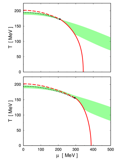
Figure 17: (Color online) $\mu-T$ phase diagrams for the parametrization given in Sec. 3.3, taking $\eta=0$ (upper panel) and $\eta=0.5$ (lower panel). The results correspond to a polynomial PL potential, with $T_{0}=208$ MeV. First order chiral restoration transitions are indicated by solid lines, while dashed and dotted lines correspond to chiral restoration and deconfinement crossover-like transitions, respectively. The green bands indicate the regions in which $0.3\leq\Phi\leq 0.5$.

The effect of the value of the parameter $\eta$ on the phase diagram can be observed by comparing the upper and lower panels of Fig. 17. As stated, this parameter measures the relative strength of the $J=1$ isoscalar couplings in comparison with their isovector counterparts. As expected, it is seen that the effect of the isoscalar piece increases with the chemical potential. In particular, when $\eta$ is enhanced the CEP moves towards lower temperatures and higher chemical potentials, and the critical value $\mu_{c}(T=0)$ gets larger. The results for various critical temperatures and chemical potentials, considering $\eta=0$, 0.3 and 0.5 are summarized in Table 7. Qualitative similar results for the phase diagram have been found in Ref. Contrera:2012wj for a logarithmic PL potential. In addition, a more complete analysis of the existence and position of the CEP within nonlocal models that include the couplings between isoscalar $J=1$ quark currents can be found in Ref. Contrera:2016rqj . Regarding the case of imaginary chemical potential, it has been argued Kashiwa:2011td that the isoscalar vector interactions can have some effect on the location of the RW end point and the pattern of transition lines in its neighborhood.

	$\eta=0$	$\eta=0.3$	$\eta=0.5$
$T_{\rm ch}(0)$	202	202	202
$T_{\Phi}(0)$	194	194	194
$T_{\rm CEP}$	173	166	156
$\mu_{\rm CEP}$	209	252	295
$\mu_{c}(0)$	343	366	388

Table 7: Critical temperatures and chemical potentials for various values of $\eta$. Values are given in MeV

3.5 Thermal behavior of meson properties

The thermal evolution of meson masses and decay constants in the context of the nlPNJL models studied in this section can be obtained by following similar steps as those outlined in Sec. 2.7. In Fig. 18 we show the numerical results obtained in Ref. Carlomagno:2019yvi for the masses of $J=0$ chiral partners $\sigma$ and $\pi$, as well as $J=1$ mesons $\rho$ and a₁. It is seen that $\pi$ and $\rho$ meson masses (solid lines) remain approximately constant up to the critical temperature $T_{\rm ch}$, while $\sigma$ and a₁ meson masses (dashed lines) start to drop somewhat below $T_{\rm ch}$. As expected from chiral restoration, right above the critical temperature chiral partner masses become degenerate. When the temperature is further increased, the masses rise continuously, showing that they are basically dominated by thermal energy.

Finally, the thermal behavior of $f_{\pi}$ and $f_{v}$ decay form factors is shown in Fig. 19. It is seen that both quantities remain constant up to approximately the chiral restoration critical temperature, and then they show a sudden drop. For large temperatures both $f_{\pi}$ and $f_{v}$ tend to zero, at different rates.

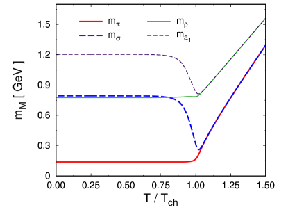
Figure 18: Meson masses as functions of the temperature.

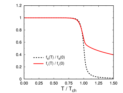
Figure 19: Normalized $f_{\pi}$ and $f_{v}$ decay form factors as functions of the temperature.

4 Three-flavor nonlocal NJL models

In this Section we review the extension of nonlocal NJL models to three dynamical quark flavors. This has been firstly addressed in Ref. Scarpettini:2003fj for the case of vanishing temperature and chemical potential, and then extended to finite temperature —including the coupling to the Polyakov loop— in Ref. Contrera:2007wu . In those works, the scheme based on the instanton liquid model has been considered (see the discussion in Sec. 2.1.1). In the case of the nlNJL approach inspired on one gluon exchange interactions, three-flavor models have been firstly analyzed in Refs. Hell:2009by ; Contrera:2009hk .

4.1 Three-flavor nlNJL model at vanishing temperature and chemical potential

4.1.1 Effective action

Let us consider a three-flavor extension of the model studied in Sec. 2, which includes quark WFR interactions. The corresponding Euclidean effective action, proposed in Ref. Carlomagno:2013ona , reads

$$S_{E} = \int d^{4}x\ \left\{\bar{\psi}(x)(-i\not{\partial}+\hat{m})\psi(x)-\frac{G_{S}}{2}\left[j^{a}_{S}(x)j^{a}_{S}(x)+j^{a}_{P}(x)j^{a}_{P}(x)+j_{R}(x)j_{R}(x)\right]\right.$$ (93)

$$\left.-\frac{H}{4}A_{abc}\left[j^{a}_{S}(x)j^{b}_{S}(x)j^{c}_{S}(x)-3j^{a}_{S}(x)j^{b}_{P}(x)j^{c}_{P}(x)\right]\right\}\ ,$$

where $\psi$ is the $u$, $d$, $s$ quark triplet and $\hat{m}={\rm diag}(m_{u},m_{d},m_{s})$ is the current quark mass matrix. As in the two-flavor case, we consider the isospin symmetry limit, assuming $m_{u}=m_{d}$. The nonlocal quark-antiquark currents are now given by

$$j^{a}_{S}(x) = \int d^{4}z\;\mathcal{G}(z)\,\bar{\psi}\left(x+\frac{z}{2}\right)\lambda_{a}\,\psi\left(x-\frac{z}{2}\right)\ ,$$

$$j^{a}_{P}(x) = \int d^{4}z\;\mathcal{G}(z)\,\bar{\psi}\left(x+\frac{z}{2}\right)i\,\lambda_{a}\gamma_{5}\,\psi\left(x-\frac{z}{2}\right)\ ,$$

$$j_{R}(x) = \int d^{4}z\;\mathcal{F}(z)\,\bar{\psi}\left(x+\frac{z}{2}\right)\frac{i\overleftrightarrow{\not{\partial}}}{2\varkappa_{p}}\,\psi\left(x-\frac{z}{2}\right)\ ,$$ (94)

where $\mathcal{G}(z)$ and $\mathcal{F}(z)$ are covariant form factors, as described in Sec. 2.3, and $\lambda_{a}$, $a=0,\dots,8$, are the standard eight Gell-Mann matrices, plus $\lambda_{0}=\sqrt{2/3}\;\mathbf{1}_{3\times 3}$. As in the two-flavor case, the couplings involving scalar and pseudoscalar currents have to carry the same form factor to guarantee chiral invariance, while the coupling $j_{R}(x)j_{R}(x)$, responsible for quark WFR, is self-invariant under chiral SU(3) transformations. The relative weight of this self-invariant term is controlled by the parameter $\varkappa_{p}$. In addition, the model accounts for flavor mixing through a ’t Hooft-like term, in which the constants $A_{abc}$ are defined by

$$A_{abc}\ =\ \frac{1}{3!}\epsilon_{ijk}\epsilon_{mnl}(\lambda_{a})_{im}(\lambda_{b})_{jn}(\lambda_{c})_{kl}\ .$$ (95)

The role of this six-fermion coupling, which is obtained from a determinant in flavor space, is to break the U(1)_A symmetry, not observed in nature.

As stated in the previous sections, in order to deal with meson degrees of freedom it is convenient to perform a bosonization of the fermionic theory. In the present case this can be done by introducing scalar fields $\sigma_{a}(x)$ and $\zeta(x)$ and pseudoscalar fields $\pi_{a}(x)$, together with auxiliary fields $S_{a}(x)$, $P_{a}(x)$ and $R(x)$, with $a=0,\dots,8$. After integrating out the fermion fields one obtains a partition function of the form

$$\mathcal{Z} = \int{\rm D}\sigma_{a}\,{\rm D}\pi_{a}\,{\rm D}\zeta\ \ {\rm det}\,{\cal D}\ \int{\rm D}S_{a}\,{\rm D}P_{a}\,{\rm D}R\ \exp\Bigg{[}\int d^{4}x\ \bigg{(}\sigma_{a}S_{a}\,+\,\pi_{a}P_{a}\,+\,\zeta R$$ (96)

$$\quad+\;\frac{G_{S}}{2}(S_{a}S_{a}+P_{a}P_{a}+R^{2})\;+\;\frac{H}{4}A_{abc}(S_{a}S_{b}S_{c}-3S_{a}P_{b}P_{c})\bigg{)}\Bigg{]}\ .$$

Here, the operator ${\cal D}$ —in momentum space— is given by

$$\!\!\!\!{\cal D}(p,p^{\prime}) = (2\pi)^{4}\delta^{(4)}(p-p^{\prime})(\not{p}+\hat{m})$$ (97)

$$+\,g\left(\frac{p+p^{\prime}}{2}\right)\Big{[}\sigma_{a}(p-p^{\prime})+i\,\gamma_{5}\pi_{a}(p-p^{\prime})\Big{]}\lambda_{a}\,-\,f\left(\frac{p+p^{\prime}}{2}\right)\frac{\not{p}+\not{p}^{\prime}}{2\varkappa_{p}}\zeta(p-p^{\prime})\ ,$$

where, as in the two-flavor case, $g(p)$ and $f(p)$ denote the Fourier transforms of the form factors $\mathcal{G}(z)$ and $\mathcal{F}(z)$.

4.1.2 Mean field approximation and chiral quark-antiquark condensates

We consider the mean field approximation (MFA), in which scalar and pseudoscalar fields are expanded around homogeneous vacuum expectation values, viz.

$$\sigma_{a}(x) = \bar{\sigma}_{a}+\delta\sigma_{a}(x)\ ,$$

$$\pi_{a}(x) = \delta\pi_{a}(x)\ ,$$

$$\zeta(x) = \bar{\zeta}+\delta\zeta(x)\ .$$ (98)

As usual, it is assumed that pseudoscalar mean field values vanish, owing to parity conservation. Moreover, in the scalar field sector only $\bar{\sigma}_{0}$, $\bar{\sigma}_{8}$ and $\bar{\zeta}$ are taken to be different from zero, due to charge and isospin symmetries.

Following the stationary phase approximation, the path integral over the auxiliary fields can be replaced by the corresponding integrand, evaluated at the values $\tilde{S}_{a}$, $\tilde{P}_{a}$, and $\tilde{R}$ that minimize the argument of the exponential in Eq. (96) Scarpettini:2003fj . In this way, the Euclidean action per unit volume reduces to

$$\frac{S_{E}^{\rm MFA}}{V^{(4)}}\ =\ -\,\int\frac{d^{4}p}{(2\pi)^{4}}\;{\rm Tr}\,\ln{\cal D}_{0}(p)-\bar{\sigma}_{a}\bar{S}_{a}-\bar{\zeta}\bar{R}-\frac{G_{S}}{2}(\bar{S}_{a}\bar{S}_{a}+\bar{R}^{2})-\frac{H}{4}A_{abc}\bar{S}_{a}\bar{S}_{b}\bar{S}_{c}\ ,$$ (99)

where $\bar{S}_{a}$, $\bar{P}_{a}$ and $\bar{R}$ stand for the values of $\tilde{S}_{a}$, $\tilde{P}_{a}$ and $\tilde{R}$ within the MFA. In the first term on the right hand side one has

$${\cal D}_{0}(p)\ =\ \left[1-\frac{\bar{\zeta}}{\varkappa_{p}}f(p)\right]\not{p}\,+\,\hat{m}\,+\,g(p)\Big{(}\bar{\sigma}_{0}\lambda_{0}+\bar{\sigma}_{8}\lambda_{8}\Big{)}\ ,$$ (100)

and the trace is taken over color, flavor and Dirac indices.

For the neutral fields ($a=0,3,8$) it is convenient to change to a flavor basis, $\phi_{a}\to\phi_{i}$, where $i=u,d,s$, or equivalently $i=1,2,3$. In this basis, by minimizing the mean field action in Eq. (99) one obtains the gap equations

$$\bar{\sigma}_{u}+G_{S}\bar{S}_{u}+\frac{H}{2}\bar{S}_{d}\bar{S}_{s} = 0\ ,$$

$$\bar{\sigma}_{d}+G_{S}\bar{S}_{d}+\frac{H}{2}\bar{S}_{s}\bar{S}_{u} = 0\ ,$$

$$\bar{\sigma}_{s}+G_{S}\bar{S}_{s}+\frac{H}{2}\bar{S}_{u}\bar{S}_{d} = 0\ ,$$ (101)

plus an extra equation arising from the $j_{R}(x)$ current-current interaction, namely

$$\bar{\zeta}\,+\,G_{S}\,\bar{R}\ =\ 0\ .$$ (102)

The mean field values $\bar{S}_{i}$ and $\bar{R}$ are given by

$$\bar{S}_{i} = -8N_{c}\int\frac{d^{4}p}{(2\pi)^{4}}\ g(p)\;\frac{Z(p)\,M_{i}(p)}{D_{i}(p)}\ ,$$

$$\bar{R} = \frac{4N_{c}}{\varkappa_{p}}\sum_{i=1}^{3}\int\frac{d^{4}p}{(2\pi)^{4}}\ p^{2}\,f(p)\;\frac{Z(p)}{D_{i}(p)}\ ,$$ (103)

where we have defined $D_{i}(p)=p^{2}+M_{i}(p)^{2}$. As in the two-flavor case [see Eq. (12)], the functions $M_{i}(p)$ and $Z(p)$ correspond to the momentum-dependent effective masses and WFR of quark propagators. They are related to the nonlocal form factors through

$$M_{i}(p) = Z(p)\,\Big{[}m_{i}\,+\,\bar{\sigma}_{i}\;g(p)\Big{]}\ ,$$

$$Z(p) = \left[1\,-\,\frac{\bar{\zeta}}{\varkappa_{p}}\,f(p)\right]^{-1}\ .$$ (104)

Thus, for a given set of model parameters and form factors, from Eqs. (101-104) one can numerically obtain the mean field values $\bar{\sigma}_{i}$ and $\bar{\zeta}$. As expected from isospin symmetry, one has $\bar{S}_{u}=\bar{S}_{d}$ and $\bar{\sigma}_{u}=\bar{\sigma}_{d}$.

4.1.3 Meson masses and decay constants

As in the two-flavor case (see Sec. 2.1), to analyze the properties of meson fields it is necessary to go beyond the MFA, considering quadratic fluctuations in the Euclidean action,

$$S_{E}^{\rm quad} = \dfrac{1}{2}\int\frac{d^{4}q}{(2\pi)^{4}}\sum_{M}\ r_{M}\ G_{M}(q^{2})\ \phi_{M}(q)\,\bar{\phi}_{M}(-q)\ .$$ (105)

Here, the meson fluctuations $\delta\sigma_{a}$ and $\delta\pi_{a}$ in Eq. (98) have been translated to a charge basis $\phi_{M}$, $M$ being the scalar and pseudoscalar mesons in the lowest mass nonets, plus the $\zeta$ field. The coefficient $r_{M}$ is 1 for charge eigenstates $M={\rm a}_{0}^{0}$, $\sigma$, $f_{0}$, $\zeta$, $\pi^{0}$, $\eta$ and $\eta^{\prime}$, and 2 for $M={\rm a}_{0}^{+}$, $K_{0}^{\ast+}$, $K_{0}^{\ast 0}$, $\pi^{+}$, $K^{+}$ and $K^{0}$. Analogously to Eq. (22), meson masses are given by the equations

$$G_{M}(-m_{M}^{2})\ =\ 0\ .$$ (106)

In addition, physical states have to be normalized through

$$\tilde{\phi}_{M}(q)=Z_{M}^{-1/2}\ \phi_{M}(q)\ ,$$ (107)

where the meson renormalization constants $Z_{M}$ and the associated on-shell quark-meson coupling constants $g_{Mq\bar{q}}$ are given by

$$Z_{M}^{-1}=g_{Mq\bar{q}}^{-2}\ =\ \frac{dG_{M}(q^{2})}{dq^{2}}\bigg{|}_{q^{2}=-m_{M}^{2}}\ .$$ (108)

The functions $G_{M}(q^{2})$ can be written in terms of the coupling constants $G_{S}$ and $H$, the mean field values $\bar{S}_{u,s}$ and quark loop functions that prove to be ultraviolet convergent owing to the asymptotic behavior of the nonlocal form factors. For the pseudoscalar meson sector, the $\pi$ and $K$ mesons decouple, while the $I=0$ states get mixed. In the case of the scalar fields, the ${\rm a}_{0}$ and $K_{0}^{\ast}$ mesons decouple, while the $\zeta$, $\sigma_{0}$ and $\sigma_{8}$ states get mixed by a $3\times 3$ matrix [see Eq. (115) below].

The explicit expressions for the functions $G_{M}(q^{2})$ in the context of nlNJL models with quark WFR have been quoted in Ref. Carlomagno:2013ona . For the $I\neq 0$ states $\pi$, ${\rm a}_{0}$, $K$ and $K_{0}^{\ast}$ one has

$$G_{\binom{\pi}{{\rm a}_{0}}}(q^{2}) = (G_{S}\pm\frac{H}{2}\bar{S}_{s})^{-1}+4\,C_{uu}^{\mp}(q^{2})\ ,$$

$$G_{\binom{K}{K_{0}^{\ast}}}(q^{2}) = (G_{S}\pm\frac{H}{2}\bar{S}_{u})^{-1}+4\,C_{us}^{\mp}(q^{2})\ ,$$ (109)

where the functions $C_{ij}^{\mp}(q^{2})$, with $i,j=u$ or $s$ are defined as

$$C_{ij}^{\mp}(q^{2}) = -\,2\,N_{c}\int\frac{d^{4}p}{(2\pi)^{4}}\ g(p)^{2}\;\frac{Z(p^{+})}{D_{i}(p^{+})}\ \frac{Z(p^{-})}{D_{j}(p^{-})}\ [p^{+}\cdot p^{-}\pm M_{i}(p^{+})M_{j}(p^{-})]\ ,$$ (110)

with $p^{\pm}=p\pm q/2$. At the $I=0$ pseudoscalar sector one has a mixing between the $\eta_{0}$ and $\eta_{8}$ fields. The masses of the physical states $\eta$ and $\eta^{\prime}$ can be obtained from the functions

$$G_{\binom{\eta}{\eta^{\prime}}}(q^{2})\ =\ \frac{G_{88}^{-}(q^{2})+G_{00}^{-}(q^{2})}{2}\mp\sqrt{[G_{80}^{-}(q^{2})]^{2}+\left(\frac{G_{88}^{-}(q^{2})-G_{00}^{-}(q^{2})}{2}\right)^{2}}\ ,$$ (111)

where we have used the definitions

$$G_{00}^{\mp}(q^{2}) = \frac{4}{3}\left[2C_{uu}^{\mp}(q^{2})+C_{ss}^{\mp}(q^{2})+\frac{6G_{S}\mp H\bar{S}_{s}\pm 4H\bar{S}_{u}}{8G_{S}^{2}-4H^{2}\bar{S}_{u}^{2}\mp 4HG_{S}\bar{S}_{s}}\right]\ ,$$

$$G_{88}^{\mp}(q^{2}) = \frac{4}{3}\left[2C_{ss}^{\mp}(q^{2})+C_{uu}^{\mp}(q^{2})+\frac{6G_{s}\mp 2H\bar{S}_{s}\mp 4H\bar{S}_{u}}{8G_{S}^{2}-4H^{2}\bar{S}_{u}^{2}\mp 4HG_{S}\bar{S}_{s}}\right]\ ,$$

$$G_{80}^{\mp}(q^{2}) = \frac{4}{3}\sqrt{2}\left[C_{uu}^{\mp}(q^{2})-C_{ss}^{\mp}(q^{2})\pm\frac{H(\bar{S}_{s}-\bar{S}_{u})}{8G_{S}^{2}-4H^{2}\bar{S}_{u}^{2}\mp 4HG_{S}\bar{S}_{s}}\right]\ .$$ (112)

The states $\eta$ and $\eta^{\prime}$ are defined as

$$\eta = \eta_{8}\cos\theta_{\eta}-\eta_{0}\sin\theta_{\eta}\ ,$$

$$\eta^{\prime} = \eta_{8}\sin\theta_{\eta}^{\prime}+\eta_{0}\cos\theta_{\eta}^{\prime}\ ,$$ (113)

where the mixing angles $\theta_{\eta}$, $\theta_{\eta^{\prime}}$ are given by

$$\tan 2\,\theta_{\eta,\eta^{\prime}}=\frac{-2G_{80}^{-}(q^{2})}{G_{88}^{-}(q^{2})-G_{00}^{-}(q^{2})}\bigg{|}_{q^{2}=-m^{2}_{\eta,\eta^{\prime}}}\ .$$ (114)

Finally, for the $I=0$ scalar sector, the quadratic terms involving the fields $\zeta$, $\sigma_{0}$ and $\sigma_{8}$ are mixed by the $3\times 3$ matrix

$$\left(\begin{array}[]{ccc}4\,C^{\zeta}(q^{2})+G_{S}^{-1}&\sqrt{\frac{8}{3}}[2\,C_{u}^{+\zeta}(q^{2})+C_{s}^{+\zeta}(q^{2})]&\frac{4}{\sqrt{3}}[C_{u}^{+\zeta}(q^{2})-C_{s}^{+\zeta}(q^{2})]\\ \sqrt{\frac{8}{3}}[2\,C_{u}^{+\zeta}(q^{2})+C_{s}^{+\zeta}(q^{2})]&G_{00}^{+}(q^{2})&G_{80}^{+}(q^{2})\\ \frac{4}{\sqrt{3}}[C_{u}^{+\zeta}(q^{2})-C_{s}^{+\zeta}(q^{2})]&G_{80}^{+}(q^{2})&G_{88}^{+}(q^{2})\end{array}\right)\ ,$$ (115)

where

$$C^{\zeta}(q^{2}) = \dfrac{N_{c}}{\varkappa_{p}^{2}}\,\sum_{i=1}^{3}\int\!\!\frac{d^{4}p}{(2\pi)^{4}}\ p^{2}f(p)^{2}\;\frac{Z(p^{+})}{D_{i}(p^{+})}\ \frac{Z(p^{-})}{D_{i}(p^{-})}$$

$$\times\left[p^{+}\cdot p^{-}+\dfrac{p^{+2}p^{-2}-(p^{+}\cdot p^{-})^{2}}{2p^{2}}-M_{i}(p^{+})M_{i}(p^{-})\right]\ ,$$

$$C_{i}^{+\zeta}(q^{2}) = -\dfrac{2\,N_{c}}{\varkappa_{p}}\,\int\frac{d^{4}p}{(2\pi)^{4}}\ g(p)\,f(p)\,\frac{Z(p^{+})}{D_{i}(p^{+})}\ \frac{Z(p^{-})}{D_{i}(p^{-})}\ p\cdot\left[p^{-}\,M_{i}(p^{+})+p^{+}M_{i}(p^{-})\right]\ ,$$ (116)

with $i=u,s$. The functions $G_{\sigma}(q^{2})$, $G_{f_{0}}(q^{2})$ and $G_{\zeta}(q^{2})$ are given by the eigenvalues of this matrix. From the first two one can determine the masses of the $\sigma$ and $f_{0}$ physical states, while the function $G_{\zeta}(q^{2})$ turns out to be positive definite for real, positive values of $-q^{2}$. The corresponding mixing angles can be obtained in a similar way as for the $\eta$ meson sector, now defining SO(3) rotation matrices.

The weak decay constants of pseudoscalar mesons can be calculated following similar steps as those sketched in Sec. 2.1.3. Details of this procedure for the three-flavor case can be found in Refs. Scarpettini:2003fj ; Hell:2009by ; Carlomagno:2013ona . The weak decay constants for $\pi$ and $K$ mesons in the isospin limit are given by

$$f_{\pi} = \frac{g_{\pi q\bar{q}}}{m_{\pi}^{2}}\;F_{uu}(-m_{\pi}^{2})\ ,$$

$$f_{K} = \frac{g_{Kq\bar{q}}}{m_{K}^{2}}\;F_{us}(-m_{K}^{2})\ ,$$ (117)

where

$$F_{ij}(q^{2}) = 2N_{c}\int\frac{d^{4}p}{(2\pi)^{4}}\;\left[g(p^{+})+g(p^{-})-2g(p)\right]\,Z(p)\left[\frac{M_{i}(p)}{D_{i}(p)}\,+\,\frac{M_{j}(p)}{D_{j}(p)}\right]$$ (118)

$$-\,2N_{c}\int\frac{d^{4}p}{(2\pi)^{4}}\;(\bar{\sigma}_{i}+\bar{\sigma}_{j})\,\left[g(p^{+})+g(p^{-})-2g(p)\right]\,g(p)$$

$$\qquad\qquad\times\,\frac{Z(p^{+})}{D_{i}(p^{+})}\;\frac{Z(p^{-})}{D_{j}(p^{-})}\;\left[p^{+}\cdot p^{-}+M_{i}(p^{+})M_{j}(p^{-})\right]$$

$$+\,4N_{c}\int\frac{d^{4}p}{(2\pi)^{4}}\;g(p)\;\frac{\left[M_{i}(p^{+})p^{-}-M_{j}(p^{-})p^{+}\right]\cdot\left[Z(p^{-})p^{+}-Z(p^{+})p^{-}\right]}{D_{i}(p^{+})\,D_{j}(p^{-})}\ \ ,$$

with $p^{\pm}=p\pm q/2$. It is worth pointing out that the functions $F_{ij}$ do not depend on the arbitrary path chosen in the transport functions.

For the $\eta-\eta^{\prime}$ sector, one has

$$f_{\eta}^{a} = \frac{Z_{\eta}^{1/2}}{m_{\eta}^{2}}\left[f_{a8}(q^{2})\cos\theta_{\eta}-f_{a0}(q^{2})\sin\theta_{\eta}\right]\bigg{|}_{q^{2}=-m_{\eta}^{2}}\ ,$$

$$f_{\eta^{\prime}}^{a} = \frac{Z_{\eta^{\prime}}^{1/2}}{m_{\eta^{\prime}}^{2}}\left[f_{a8}(q^{2})\sin\theta_{\eta^{\prime}}+f_{a0}(q^{2})\cos\theta_{\eta^{\prime}}\right]\bigg{|}_{q^{2}=-m_{\eta^{\prime}}^{2}}\ ,$$ (119)

where $a=0,8$. The functions $f_{ab}(q^{2})$ are related to $F_{ij}(q^{2})$ through

$$f_{00}(q^{2}) = \frac{1}{3}\left[2F_{uu}(q^{2})+F_{ss}(q^{2})\right]\ ,$$

$$f_{88}(q^{2}) = \frac{1}{3}\left[F_{uu}(q^{2})+2F_{ss}(q^{2})\right]\ ,$$

$$f_{08}(q^{2}) = \frac{\sqrt{2}}{3}\left[F_{uu}(q^{2})-F_{ss}(q^{2})\right]\ .$$ (120)

In order to compare with phenomenological determinations, it is convenient to consider an alternative parametrization in terms of two decay constants $f_{0}$, $f_{8}$ and two mixing angles $\theta_{0}$, $\theta_{8}$ Leutwyler:1997yr ; Feldmann:1999uf . Both parametrizations are related by

$$\left(\begin{array}[]{cc}f_{\eta}^{8}&f_{\eta}^{0}\\ f_{\eta^{\prime}}^{8}&f_{\eta^{\prime}}^{0}\end{array}\right)\ =\ \left(\begin{array}[]{cc}f_{8}\cos\theta_{8}&-f_{0}\sin\theta_{0}\\ f_{8}\sin\theta_{8}&f_{0}\cos\theta_{0}\end{array}\right)\ .$$ (121)

4.2 Extension to finite temperature and chemical potential. Coupling with the Polyakov loop

In this subsection we analyze the predictions of three-flavor nonlocal models for a system at finite temperature $T$ and/or quark chemical potential $\mu$. The formalism presented in Sec. 4.1 can be extended to nonzero $T$ and $\mu$ following the prescriptions described in Sec. 2.2 for the two-flavor case. This includes the couplings between the quarks and the Polyakov loop and the effective potential $\mathcal{U}(\Phi,\Phi^{\ast},T)$ that accounts for color gauge self-interactions. The grand canonical thermodynamic potential per unit volume within the MFA is given by Contrera:2007wu ; Hell:2009by ; Carlomagno:2013ona

$$\Omega^{\rm MFA}_{\rm reg}\ =\ \Omega^{\rm MFA}\,-\,\Omega^{\rm free}_{q}\,+\,\Omega^{\rm free}_{q,{\rm reg}}\,+\,\Omega_{0}\ ,$$ (122)

where

$$\Omega^{\rm MFA}-\Omega^{\rm free}_{q} = -\,2\,\sum_{c,f}\ T\sum_{n=-\infty}^{\infty}\int\dfrac{d^{3}p}{(2\pi)^{3}}\ln\left[\dfrac{(\rho_{n,\vec{p}}^{c})^{2}+M_{f}(\rho_{n,\vec{p}}^{c})^{2}}{Z(\rho_{n,\vec{p}}^{c})^{2}\,[(\rho_{n,\vec{p}}^{c})^{2}+m^{2}_{f}]}\right]$$

$$-\left(\bar{\zeta}\,\bar{R}+\dfrac{G_{S}}{2}\,\bar{R}^{2}+\dfrac{H}{4}\,\bar{S}_{u}\,\bar{S}_{d}\,\bar{S}_{s}\right)-\dfrac{1}{2}\,\sum_{f}\left(\bar{\sigma}_{f}\bar{S}_{f}+\dfrac{G_{S}}{2}\,\bar{S}_{f}^{2}\right)$$

$$+\,\ \mathcal{U}(\Phi,\Phi^{\ast},T)\ ,$$

$$\Omega^{\rm free}_{q,{\rm reg}} = -2\,T\sum_{c,f}\sum_{s=\pm 1}\int\dfrac{d^{3}p}{(2\pi)^{3}}\;{\rm Re}\,\ln\left[1+\exp\left(-\frac{\epsilon_{fp}+s\,(\mu\,+i\,\phi_{c})}{T}\right)\right]\ .$$ (123)

Here we have used the definition in Eq. (38), viz. $(\rho_{n,\vec{p}}^{c})^{2}=\vec{p}^{\,2}+[(2n+1)\pi T+i\mu-\phi_{c}]^{2}$, while the free quark energies are given by $\epsilon_{fp}=\sqrt{\vec{p}^{\;2}+m_{f}^{2}}$. The sums over color and flavor indices run over $c=r,g,b$ and $f=u,d,s$, respectively. As discussed in Sec. 2.3, the color background fields $\phi_{c}$ can be written in terms of a single field $\phi_{3}$ (the other independent field, $\phi_{8}$, is taken to be zero since in this section we deal with real values of the chemical potential). We recall that $\Omega_{0}$ is a constant that fixes to zero the thermodynamic potential at $T=\mu=0$. From the minimization of $\Omega^{\rm MFA}_{\rm reg}$ it is possible to obtain a set of coupled gap equations that determine the mean field values of the scalar fields, as well as the traced Polyakov loop, at a given temperature $T$ and chemical potential $\mu$.

To characterize the chiral and deconfinement phase transitions it is necessary to define the corresponding order parameters. As stated, the chiral quark condensates $\langle\bar{q}q\rangle$ are appropriate order parameters for the restoration of the chiral symmetry. Their expressions can be obtained by varying the regularized thermodynamic potential with respect to the current quark masses. In general, the corresponding quark loop integrals are divergent, and can be regularized by subtracting the free quark contributions as in Eq. (20). For the three-flavor case it is usual to define a subtracted chiral condensate normalized to its value at $T=0$ according to

$$\langle\bar{q}q\rangle_{\rm sub}\ =\ \dfrac{\langle\bar{u}u\rangle\,-\,\frac{m_{u}}{m_{s}}\,\langle\bar{s}s\rangle}{\langle\bar{u}u\rangle_{0}\,-\,\frac{m_{u}}{m_{s}}\,\langle\bar{s}s\rangle_{0}}\ .$$ (124)

In addition, from the thermodynamic potential we can also calculate various thermodynamic quantities such as the pressure, the entropy and the energy density, which are given by

$$p\ =\ -\Omega^{\rm MFA}_{\rm reg}\ ,\qquad\qquad s\ =\ -\,\dfrac{\partial\Omega^{\rm MFA}_{\rm reg}}{\partial T}\ ,\qquad\qquad\varepsilon\ =\ \Omega^{\rm MFA}_{\rm reg}+T\;s\ .$$ (125)

4.3 Form factors, parametrizations and numerical results for $T=\mu=0$

The three-flavor action in Eq. (93) includes five free parameters, namely the current quark masses $m_{u}$ and $m_{s}$, and the coupling constants $G_{S}$, $H$ and $\varkappa_{p}$. In addition, one has to specify the nonlocal form factors $g(p)$ and $f(p)$. As in the case of two-flavor models, we take into account two types of functions for these form factors. The first parametrization, PI, considers the often used exponential forms, which guarantee a fast ultraviolet convergence of the loop integrals. For the second one, PII, we consider a momentum dependence based on lattice QCD results for quark propagators Carlomagno:2013ona . The corresponding explicit expressions are given by Eqs. (48) and (50-52) in Sec. 2.3, where the parametrizations are denoted as PB and PC, respectively.

Taking into account the nonlocal form factors, one has to add to the above mentioned free parameters the effective momentum cutoff scales $\Lambda_{0}$ and $\Lambda_{1}$. Then, to determine the full parameter sets, one can require that the model be able to reproduce the empirical values of some physical quantities. Following Refs. Carlomagno:2013ona ; Carlomagno:2018tyk these are taken to be the masses of the pseudoscalar mesons $\pi$, $K$ and $\eta^{\prime}$, and the pion weak decay constant $f_{\pi}$. In the case of PI Carlomagno:2013ona , the additional three input values are the current quark mass $m_{u}$, the value of the quark wave function renormalization $Z(p)$ at $p=0$ and the chiral quark condensate $\langle\bar{q}q\rangle$, $q=u,d$, which is fixed to $\langle\bar{q}q\rangle=(-240\ {\rm MeV})^{3}$. For the lattice-inspired parametrization PII, input values for $\Lambda_{0}$, $\Lambda_{1}$ and $\alpha_{z}$ [or, equivalently, $Z(0)$] are obtained through a fit to LQCD results quoted in Ref. Parappilly:2005ei for the functions $Z(p)$ and $f_{m}(p)$ given in Eqs. (50) and (51). This fit leads to $\Lambda_{0}=861$ MeV, $\Lambda_{1}=1728$ MeV and $\alpha_{z}=-0.249$ Carlomagno:2018tyk . The numerical values for the model parameters, for both PI and PII, are quoted in Table 8. The curves corresponding to the functions $f_{m}(p)$ and $Z(p)$ for both parametrizations, together with $N_{f}=2+1$ LQCD results from Ref. Parappilly:2005ei , are shown in Fig. 20.

		PI	PII
$m_{u}$	MeV	$5.7$	$2.4$
$m_{s}$	MeV	$136$	$61.5$
$G_{S}\Lambda_{0}^{2}$		$23.64$	$14.03$
$H\Lambda_{0}^{5}$		$-526$	$-159$
$\varkappa_{p}$	GeV	$4.36$	$10.76$
$\Lambda_{0}$	MeV	$814$	$861$
$\Lambda_{1}$	MeV	$1032$	$1728$

Table 8: Values of model parameters for PI Carlomagno:2013ona and PII Carlomagno:2018tyk .

(a)

(b)

Figure 20: (Color online) Quark propagator functions $f_{m}(p)$ (left) and $Z(p)$ (right). Dashed and solid lines correspond to parametrizations PI, Eq. (49), and PII, Eq. (50), respectively. Lattice results from Ref. Parappilly:2005ei are indicated by the black dots.

After fixing the model parametrization, it is possible to calculate the mean field values of the scalar fields, as well as to obtain predictions for various physical quantities. In Table 9 we quote the numerical results for the mean field values $\bar{\sigma}_{u}$, $\bar{\sigma}_{s}$ and $\bar{\zeta}$, together with the $u$- and $s$-quark condensates. In the same way as in the two-flavor case (see Tables 1 and 2), for PII one obtains relatively low values for the current quark masses and large values for the quark condensates Noguera:2008cm ; Hell:2011ic ; Carlomagno:2013ona . As discussed in Sec. 2.3, this can be understood by noticing that PII is based on a fit to LQCD results that correspond to a renormalization scale of 3 GeV. In any case, for both PI and PII one gets a phenomenologically adequate quark mass ratio $m_{u}/m_{s}\sim 1/25$. Moreover, the product $-\langle\bar{u}u\rangle m_{u}$ is found to be about $8\times 10^{-5}$ GeV⁴, in agreement with the scale-independent result obtained from the Gell-Mann-Oakes-Renner relation, Eq. (30), namely $-\langle\bar{u}u\rangle m_{u}=f_{\pi}^{2}m_{\pi}^{2}/2\simeq 8.3\times 10^{-5}$ GeV⁴.

		PI	PII
$\bar{\sigma}_{u}$	MeV	$529$	$400$
$\bar{\sigma}_{s}$	MeV	$702$	$630$
$\bar{\zeta}/\varkappa_{p}$		$-0.429$	$-0.332$
$-\langle\bar{u}u\rangle^{1/3}$	MeV	$240$	$325$
$-\langle\bar{s}s\rangle^{1/3}$	MeV	$198$	$358$

Table 9: Numerical results for mean field values of scalar fields and chiral quark condensates.

Finally, in Table 10 we summarize the numerical results obtained for meson masses, decay constants and mixing angles Carlomagno:2013ona ; Carlomagno:2018tyk . For comparison, we also include the corresponding phenomenological estimates. Notice that quantities chosen as inputs are marked with an asterisk. In the case of the $I=0$ scalar particles, the masses have been obtained by determining the zeroes of the functions $G_{M}(p^{2})$ arising from the diagonalization of the $3\times 3$ matrix in Eq. (115). As stated, from the corresponding numerical calculations it is seen that one of these functions is positive definite for the whole momentum range described by the model. Therefore, the corresponding eigenstate cannot be associated to a light physical meson. The remaining two states can be identified with the $\sigma$ (or $f_{0}(500)$) and $f_{0}(980)$ scalar mesons quoted by the Particle Data Group Zyla:2020zbs . Analogously, the masses of $K_{0}^{\ast}$ charged and neutral states can be identified with the $K_{0}^{\ast}(1430)$ mesons Zyla:2020zbs . By comparing with the phenomenological values, it is seen that in general the predictions of the model for both PI and PII are in a reasonable agreement with phenomenological expectations. Some numerical results for three-flavor nlNJL schemes that consider other form factor functions and/or parameter sets can be found in Refs. Scarpettini:2003fj ; Hell:2009by ; Hell:2011ic .

		PI	PII	Empirical
$m_{\pi}$	MeV	$139$ ∗	$139$ ∗	$139$
$m_{\sigma}$	MeV	$599$	$518$	400 - 550
$m_{K}$	MeV	$495$ ∗	$495$ ∗	$495$
$m_{K_{0}^{\ast}}$	MeV	$1300$	$1159$	$1425$
$m_{\eta}$	MeV	$527$	$511$	$547$
$m_{{\rm a}_{0}}$	MeV	$936$	$968$	$980$
$m_{\eta^{\prime}}$	MeV	$958$ ∗	$958$ ∗	$958$
$m_{{\rm f}_{0}}$	MeV	$1300$	$1280$	$990$
$f_{\pi}$	MeV	$92.4$ ∗	$92.4$ ∗	$92.4$
$f_{K}/f_{\pi}$		$1.17$	$1.18$	$1.22$
$f_{\eta}^{0}/f_{\pi}$		$0.17$	$0.27$	$(0.11$ - $0.51)$
$f_{\eta}^{8}/f_{\pi}$		$1.12$	$1.05$	$(1.17$ - $1.22)$
$f_{\eta^{\prime}}^{0}/f_{\pi}$		$1.09$	$2.12$	$(0.98$ - $1.16)$
$f_{\eta^{\prime}}^{8}/f_{\pi}$		$-0.48$	$-0.63$	$-(0.42$ - $0.46)$
$\theta_{0}$	deg	$-8.6$	$-7$	$-(10$ - 12)
$\theta_{8}$	deg	$-23$	$-31$	$-(25$ - 29)

Table 10: Numerical results for various phenomenological quantities. Input values are marked with an asterisk.

4.4 Results for finite temperature and vanishing chemical potential

In the framework of the three-flavor nlPNJL models introduced above, we present here some results for physical quantities at finite temperature and $\mu=0$. We consider the parametrizations PI and PII defined in the previous subsection, and the Polyakov loop potentials introduced in Sec. 2.2. Fig. 21 illustrates the behavior of the order parameters for deconfinement and SU(2) chiral symmetry restoration transitions, namely the traced Polyakov loop $\Phi$ and the subtracted chiral condensate $\langle\bar{q}q\rangle_{\rm sub}$, as well as the associated susceptibilities, as functions of the temperature. The curves correspond to parametrization PII Carlomagno:2018tyk . In the upper panel, we show the results for $\langle\bar{q}q\rangle_{\rm sub}$ (solid lines) and the traced Polyakov loop $\Phi$ (dashed lines). Thin and thick lines correspond to logarithmic and polynomial PL potentials, respectively, with $T_{0}=200$ MeV. For comparison we also include LQCD data quoted in Refs. Borsanyi:2010bp ; Bazavov:2010sb . As expected, it is found that when the temperature is increased the system undergoes both chiral restoration and deconfinement transitions, which proceed as smooth crossovers. As discussed in Sec. 2.4 for the case of two-flavor nlPNJL models, the curves for the order parameters get steeper for lower values of $T_{0}$. Indeed, for the three-flavor model, the transitions are found to be of first order for $T_{0}<185$ MeV. In the central and lower panels of Fig. 21 we display the curves for the PL and chiral susceptibilities, defined by $\chi_{\Phi}=d\Phi/dT$ and $\chi_{q}=d\langle\bar{q}q\rangle/dT$ ($q=u,s$), as functions of the temperature [for clarity, the graphs show the subtracted susceptibilities $\bar{\chi}_{q}\equiv\chi_{q}(T)-\chi_{q}(0)$]. As usual, the deconfinement and chiral restoration critical temperatures are defined by the peaks of $\chi_{\Phi}$ and $\chi_{u}$, respectively. In addition, in the curves for $\chi_{s}$ it is possible to identify a second, broad peak that allows one to define an approximate critical temperature for the restoration of the full SU(3) chiral symmetry.

Figure 21: (Color online) Order parameters and susceptibilities as functions of the temperature, for parametrization PII. Triangles, circles and squares stand for lattice QCD results from Refs. Borsanyi:2010bp ; Bazavov:2010sb .

It is seen that both the SU(2) chiral restoration and deconfinement transitions occur essentially at the same critical temperatures, in agreement with lattice QCD findings. From the curves in Fig. 21 one gets $T_{\rm ch}\simeq 165$ MeV (see Table 12), while LQCD analyses lead to a transition temperature of about 160 MeV for $N_{f}=2+1$ Bazavov:2018mes ; Borsanyi:2020fev . As in the two-flavor case (see Table 3), the above results, which correspond to the lattice QCD-inspired parameterization PII, are qualitatively similar to those obtained for parametrization PI, based on Gaussian form factors. To compare the predictions from both parameterizations it is useful to consider other thermodynamical quantities, as e.g. the interaction energy and the entropy. In Fig. 22 we show the numerical results for the normalized interaction energy $(\varepsilon-3p)/T^{4}$ (left) and the normalized entropy density $s/s_{SB}$ (right), where $s_{SB}=(32+21N_{f})\pi^{2}T^{3}/45$ is the entropy density in the free-particle Stefan-Boltzmann limit. Dashed and solid lines correspond to parameterizations PI and PII, respectively, for the logarithmic PL potential given by Eq. (35). We have included for comparison three sets of lattice data, taken from Refs. Bazavov:2010sb ; Bazavov:2009zn ; Borsanyi:2010cj . As in the case of two-flavor models (see Fig. 6), it can be seen that for both the interaction energy and the entropy the curves for PI show a pronounced dip at about $T\sim 300$ MeV, which is not observed in the case of PII. In order to trace the source of this effect we have also considered a third parameterization, PIII Contrera:2009hk ; Hell:2009by , in which the form factor $g(p)$ has a Gaussian shape as in PI, but the coupling driven by the currents $j_{R}(x)$ is not included [i.e. there is no quark WFR, $f(p)=0$, $Z(p)=1$]. This parametrization is equivalent to PA in Sec. 2.3. The results from PIII are shown by the dashed-dotted curves in Fig. 22, which do not show the mentioned dip. This indicates that, as in the two-flavor case, the effect can be attributed to the exponential behavior of the form factor $f(p)$ that leads to the quark WFR in PI. Moreover, our results can be compared with those obtained from the parameterization considered in Ref. Hell:2011ic , where the form factors are introduced so as to fit lattice results for the quark propagator (as in PII), but $f(p)$ is assumed to have a Gaussian shape. The curves for the interaction energy and the entropy for this model (indicated in Fig. 22 as PHKW, dotted lines) are similar to those obtained for the parameterization PI. Thus, taking into account lattice data, it could be stated that the choice of a power-like behavior for $f(p)$ as that proposed in Eq. (52) turns out to be more adequate than the exponential one.

Figure 22: (Color online) Normalized interaction energy (left) and entropy density (right) as functions of the temperature, for different model parameterizations. Curves correspond to nlPNJL models with logarithmic PL potentials and $T_{0}=200$ MeV. Squares, circles and triangles stand for lattice data from Ref. Bazavov:2010sb , Ref. Bazavov:2009zn and Ref. Borsanyi:2010cj , respectively. PHKW denotes the parametrization used in Ref. Hell:2011ic .

As for the general comparison with lattice QCD results, from the plots in Fig. 21 it is seen that the transition predicted by nlPNJL models is somewhat too sharp. In particular, there is an appreciable difference with lattice data in the case of the curves for the traced Polyakov loop $\Phi$ (dashed lines in the upper panel of Fig. 21). This is a general feature of Polyakov NJL-like models, both local and nonlocal, and also extends to quark-meson models. In fact, as discussed in Refs. Braun:2007bx ; Marhauser:2008fz ; Herbst:2013ufa , the strict comparison between the curves for the traced PL and lattice data has to be taken with some care, owing to the difference between the definitions of $\Phi$ in the continuum and on the lattice. One should expect a coincidence in the crossover temperatures, which in general appears to be satisfied in nlPNJL models for the potentials considered here. On the other hand, for PII the behavior of the normalized interaction energy and the entropy density (left and right panels in Fig. 22, respectively) are found to be in reasonable agreement with LQCD results. The dependence of these quantities on the PL potential is shown in Fig. 23, where the curves for PII considering both logarithmic and polynomial PL potentials are displayed, together with lattice data from Refs. Bazavov:2010sb ; Bazavov:2009zn ; Borsanyi:2010cj . It is worth mentioning that similar results for the mentioned thermodynamic quantities and order parameters have been obtained in Refs. Schaefer:2009ui ; Haas:2013qwp ; Herbst:2013ufa within the Polyakov-quark-meson model.

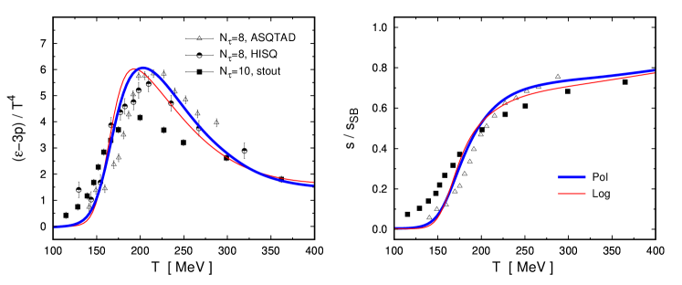
Figure 23: (Color online) Normalized interaction energy (left) and entropy density (right) as functions of the temperature for both the logarithmic and the polynomial PL potentials. Squares, circles and triangles stand for lattice data from Refs. Bazavov:2010sb ; Bazavov:2009zn ; Borsanyi:2010cj .

From the left panel of Fig. 23 it is seen that both LQCD data and nlPNJL model numerical results for the interaction energy do not tend to zero even for large temperatures. This can be interpreted as a remnant of the strong interaction in the deconfined region, signaling that the quark-gluon plasma should not be understood as a free gas of quarks and gluons. Concerning the steepness of the transitions, it is worth to mention that the behavior may be softened after the inclusion of mesonic corrections to the Euclidean action, since —as mentioned in Sec. 2.4— when the temperature is increased light meson degrees of freedom should get excited before quarks excitations emerge Blaschke:2007np ; Hell:2008cc ; Hell:2009by ; Radzhabov:2010dd . The incorporation of meson fluctuations should not modify the critical transition temperatures, which for the parametrizations considered here turn out to be in good agreement with lattice estimations.

To conclude this subsection we briefly mention some results given in Ref. Pagura:2016rit concerning the magnetic susceptibility of the QCD vacuum within nonlocal NJL models. A relevant quantity to be analyzed is the vacuum expectation value of the tensor polarization operator $\langle\bar{\psi}\,\sigma_{\mu\nu}\,\psi\rangle=\ {Q_{q}}F_{\mu\nu}\,\tau_{q}$, where $\sigma_{\mu\nu}=i[\gamma_{\mu},\gamma_{\nu}]/2$ is the relativistic spin operator, $F_{\mu\nu}$ is the electromagnetic field strength tensor, $Q_{q}$ is the quark electric charge and $\tau_{q}$ is the so-called tensor coefficient. After a somewhat long but straightforward calculation, at $T=\mu=0$ the tensor coefficient within the three-flavor nlPNJL model is found to be given by Pagura:2016rit

$$\tau_{q}\ =\ 4\,N_{c}\int\frac{d^{4}p}{(2\pi)^{4}}\ Z(p)\ \frac{M_{q}(p)-p^{2}M_{q}^{\prime}(p)}{\left[p^{2}+M_{q}(p)^{2}\right]^{2}}\ ,$$ (126)

where $q=u,d,s$ and $M_{q}^{\prime}\equiv dM_{q}(p)/dp^{2}$. In addition, one can study the magnetic susceptibilities $\chi_{q}^{\scriptsize\mbox{(cond)}}$ associated to the quark condensates. These are given by the relation $\tau_{q}=\chi^{\scriptsize\mbox{(cond)}}_{q}\langle\bar{q}q\rangle$, for $q=u,d,s$. In Table 11 we quote the values obtained for the above quantities, for parametrization PI. The results show a diamagnetic behavior for the QCD vacuum, i.e. $\chi^{\scriptsize\mbox{(cond)}}_{q}<0$. The prediction for the $u$-tensor coefficient is in good agreement with the value obtained from lattice QCD, whereas the quark magnetic susceptibilities turn out to be of the order of the corresponding LQCD estimates. On the other hand, the prediction for the $s$-tensor coefficient is significantly lower than the LQCD value. However, it can be seen Pagura:2016rit that the nlPNJL result for $\tau_{s}$ is strongly dependent on the chosen parametrization, hence the comparison of numerical values should be taken with some care in this case.

		PI	LQCD
$\tau_{u}$	MeV	38.2	40
$\tau_{s}$	MeV	9.7	53
$\chi_{u}^{\scriptsize\mbox{(cond)}}\ \$	GeV-2	$-2.77$	$-(2.05\pm 0.09)$
$\chi_{s}^{\scriptsize\mbox{(cond)}}\ \$	GeV-2	$-1.25$	$-(3.40\pm 1.40)$

Table 11: Tensor coefficients and magnetic susceptibilities for parametrization PI, compared to LQCD results from Ref. Bali:2012jv .

Following the procedure described in Sec. 2.2, the expression in Eq. (126) can be extended to finite temperature. The thermal dependence of the $u$-tensor coefficient for parametrization PI and the polynomial PL potential is shown in Fig. 24. Results for other parametrizations and PL potentials are found to be qualitative similar. A detailed comparison, which also includes the results obtained in Ref. Nam:2013wja using a ILM-inspired nonlocal model, can be found in Ref. Pagura:2016rit .

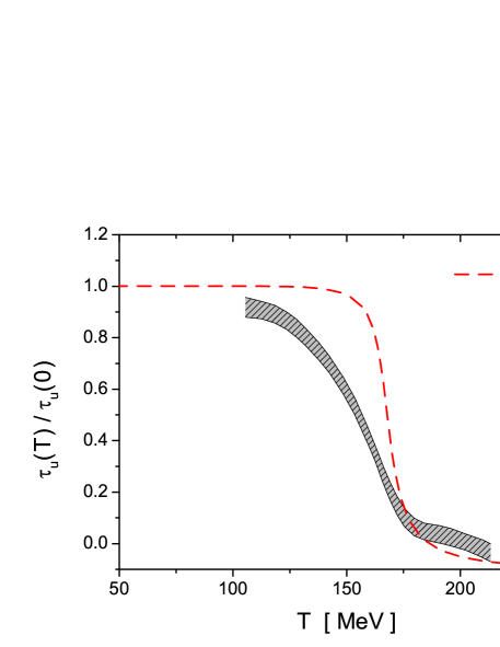
Figure 24: (Color online) Normalized $u$-quark tensor coefficient as a function of the temperature for parametrization PI, considering the polynomial PL potential. Results from LQCD Bali:2012jv are indicated by dashed gray band.

If the temperature is increased from $T=0$, it is seen that the tensor coefficient remains approximately constant up to the chiral restoration temperature $T_{\rm ch}\simeq 165$ MeV, where one finds a sudden drop. For comparison we also show the LQCD estimates from Ref. Bali:2012jv (gray dashed band). Once again, the transition predicted by the nlPNJL model seems to be somewhat too sharp, although —as in the case of thermodynamical quantities— this behavior may be softened after the inclusion of mesonic corrections to the Euclidean action.

4.5 Results at nonzero temperature and chemical potential

In this subsection we discuss the features of the phase transitions in the $\mu-T$ plane in the context of the three-flavor nlPNJL model introduced in Secs. 4.1-4.3. The phase diagram can be sketched by analyzing the numerical results obtained for the relevant order parameters. As stated, for the deconfinement and chiral symmetry restoration transitions we take as order parameters the traced Polyakov loop $\Phi$ and the subtracted chiral condensate $\langle\bar{q}q\rangle_{\rm sub}$ [defined in Eq. (124)], respectively. The associated critical temperatures $T_{\rm ch}$ and $T_{\Phi}$ are defined by the position of the peaks in the chiral susceptibilities in the region where the transition occurs as a smooth crossover. On the other hand, for relatively low temperatures the chiral restoration occurs as a first order phase transition at a given critical chemical potential $\mu_{c}(T)$. As in the case of the two-flavor model, even if this leads to a discontinuity in the order parameter $\Phi$, the latter remains close to zero after the transition, and it can be assumed that the system is still in a confined phase. Thus, we consider the prescription proposed in Sec. 2.5, defining a deconfinement transition region in which the PL lies within the range $0.3\leq\Phi\leq 0.5$.

Figure 25: (Color online) Subtracted chiral condensate (solid lines) and traced Polyakov loop (dashed lines) as functions of the temperature. Thin and thick lines correspond to the logarithmic and polynomial PL potentials, respectively.

For all parametrizations and PL potentials under consideration, one finds that for $T=0$ the chiral restoration occurs through a first order phase transition at a critical chemical potential $\mu_{c}(0)\sim 300$ MeV. If the temperature is increased, the critical chemical potential gets reduced, and the chiral transition continues to be of first order up to a certain critical end point (CEP) of coordinates $(\mu_{\rm CEP},T_{\rm CEP})$ (see Table 12). For $T>T_{\rm CEP}$, or $\mu<\mu_{\rm CEP}$, the chiral restoration phase transition proceeds as a smooth crossover. In particular, as already discussed in the previous subsection, at $\mu=0$ the system undergoes chiral restoration and deconfinement crossover-like transitions at an approximately common critical temperature $T_{\rm ch}\sim 165$ MeV (see Fig. 21), in reasonable agreement with LQCD. However, for larger values of the chemical potential (particularly for $\mu>\mu_{\rm CEP}$) these transitions might occur at different temperatures. This generic behavior is illustrated in Fig. 25, where we quote the order parameters for the deconfinement transition and the chiral symmetry restoration as functions of the temperature, considering two representative values of the chemical potential. The results in the figure correspond to parametrization PII. For $\mu=100$ MeV (upper panel) the curves are qualitatively similar to those obtained for $\mu=0$, see Fig. 21, while for $\mu=250$ MeV (larger than $\mu_{\rm CEP}$), there is a jump on $\langle\bar{q}q\rangle_{\rm sub}$ at $T\simeq 100$ MeV that signals a first order chiral restoration transition (lower panel). As discussed above, the values of $\Phi$ at the discontinuity indicate that right after the transition the system still remains in a confined phase. In fact, the deconfinement occurs at larger temperatures where $\Phi$ gets closer to one, say $T\gtrsim 150$ MeV for the chosen value of $\mu$. As already commented in Sec. 2.5, the phase in which quarks remain confined (signaled by $\Phi\lesssim 0.3$) even though chiral symmetry has been restored is usually referred to as a quarkyonic phase McLerran:2007qj ; McLerran:2008ua ; Abuki:2008nm .

The phase diagrams for three-flavor nlPNJL model parametrizations PI and PII and both logarithmic and polynomial PL potentials, taking $T_{0}=200$ MeV, are shown in Fig. 26. Solid (dashed) lines indicate first order (crossover) phase transitions for the chiral symmetry restoration, while the deconfinement transition region (defined by $0.3\leq\Phi\leq 0.5$) is denoted by the color shaded areas. The fat dots denote the position of the critical endpoints. Numerical results for CEP coordinates, critical temperatures and chemical potentials are summarized in Table 12 (values are given in MeV). As in the two-flavor case, the location of the CEP is found to be quite sensitive to the model parametrization and to the form of the PL potential. The dependence of CEP coordinates on the axial anomaly has also been studied Hell:2009by . Although nonnegligible, it is found to be less strong than that in the local PNJL model. Qualitatively similar predictions for the structure of phase diagram can be found in Ref. Rennecke:2016tkm and Ref. Schaefer:2011ex in the context of quark-meson and Polyakov-quark-meson models, respectively.

Figure 26: (Color online) Phase diagrams corresponding to parametrizations PI (upper panels) and PII (lower panels), for polynomial (left) and logarithmic (right) PL potentials. Dashed and solid lines correspond to crossover and first order chiral restoration transitions, respectively, while critical end points are indicated by the fat dots. The color shaded areas denote the deconfinement transition regions, defined by the condition $0.3\leq\Phi\leq 0.5$.

	PI			PII
	Pol	Log		Pol	Log
$T_{\rm ch}(0)$	168	164		169	163
$T_{\Phi}(0)$	166	164		167	163
$\mu_{\rm CEP}$	169	120		234	214
$T_{\rm CEP}$	145	157		112	130
$\mu_{c}(0)$	311	311		293	293

Table 12: Numerical results for some critical temperatures and chemical potentials. All values are given in MeV.

4.6 Meson properties at finite temperature

The thermal evolution of meson masses, decay constants and mixing angles in the context of three-flavor nlPNJL models has been studied in Ref. Carlomagno:2018tyk . The corresponding analytical expressions can be obtained from those given in Sec. 4.1.3 for $T=0$, following the steps sketched in Secs. 2.2 and 2.6.

The behavior is found to be qualitatively similar for all parametrizations and PL potentials under consideration Carlomagno:2018tyk , and also analogous to the one obtained within other effective theories, as the quark-meson model Rennecke:2016tkm . We quote here the results corresponding to parametrization PII, which —as shown in Sec. 4.4— provides the best agreement with lattice QCD results for thermodynamical quantities. For definiteness we consider the polynomial PL potential, Eq. (32), with $T_{0}=200$ MeV. The plots for meson masses as functions of the temperatures are displayed in Fig. 27. As shown in the upper panel, the masses of the $\pi$ and $\eta$ pseudoscalar mesons (solid lines) remain approximately constant up to the critical temperature $T_{\rm ch}$, while those of their scalar meson counterparts $\sigma$ and ${\rm a}_{0}$ (dashed lines) start dropping at somewhat lower temperatures. As expected, right above $T_{\rm ch}$ the masses of chiral partners become degenerate, while at higher temperatures they are dominated by thermal energy. In the case of the $\eta^{\prime}$ meson and its chiral partner f₀, and similarly for $K$ and $K_{0}^{\ast}$ (lower panel of Fig. 27), the degeneracy is achieved at temperatures larger than $T_{\rm ch}$. This is due to the large current mass of the strange quark, which is expected to shift the restoration of the full SU(3) chiral symmetry to higher temperatures.

Finally, in Fig. 28 we show the numerical results obtained for the thermal behavior of the pseudoscalar meson decay constants $f_{\pi}$ and $f_{K}$. The curve for $f_{\pi}$ shows a sudden drop at $T\simeq T_{\rm ch}$, similar to the one observed in two-flavor nlPNJL models (see Fig. 15). In the case of $f_{K}$ the fall is more moderate, owing to the large explicit chiral symmetry breakdown caused by the strange quark current mass.

Figure 27: (Color online) Scalar (dashed lines) and pseudoscalar (solid lines) meson masses as functions of the temperature. The results correspond to PII and a polynomial PL potential.

Figure 28: (Color online) Pion (thin line) and kaon (thick line) decay constants as functions of the temperature. The results correspond to PII and a polynomial PL potential.

5 Further developments and applications

5.1 Two-flavor superconducting quark matter and $\mu-T$ phase diagram under compact star conditions

As mentioned in the Introduction, the analysis of the phase diagram for strong-interaction matter has important applications in astrophysics. In particular, as we discuss in the next subsection, the region of low temperatures and moderate baryon chemical potentials is very interesting for the description of compact star cores Page:2006ud ; Lattimer:2015nhk . Thus, in the framework of nonlocal chiral quark models, it is worth to analyze the features of the phase diagram under compact star conditions, i.e., under the requirements of color and electric charge neutrality together with $\beta$ equilibrium Iida:2000ha ; AR02 .

An important issue to be addressed in this context is the presence of color superconducting quark matter ARW98 . In fact, a great variety of possible diquark pairing patterns has been explored in the literature, and estimations of the order of magnitude of the corresponding pairing gaps have been obtained Alford:2007xm ; Casalbuoni:2003wh . A detailed discussion on this subject within the local NJL model can be found e.g. in Ref. Buballa:2003qv . For phenomenological applications in compact stars, one relevant problem is the determination of the number of active flavors. It turns out that at low temperatures one obtains a sequential melting pattern of the light and strange quark chiral condensates, which is rather insensitive to the details of the four-momentum dependence of the interaction, but crucially dependent on a selfconsistent determination of the strange quark mass. Results obtained at the mean field level within the three-flavor local NJL model Ru05 ; Bla05 ; Abuki:2005ms indicate that under compact star conditions a two-flavor color superconducting (2SC) phase is favored over the three-flavor color-flavor-locking (CFL) one. Even if the third quark flavor occurs at not too high densities to be realized in compact star interiors, star configurations with CFL quark cores are found to be hydrodynamically unstable Baldo:2002ju . Studies of neutral 2SC quark matter consider also the presence of a so-called gapless phase SH03 ; Aguilera:2004ag , which is found to occur at intermediate temperatures and chemical potentials.

Color neutrality arises basically from the interactions between matter and color gauge fields. In NJL-like effective quark models —which do not include explicit gauge field dynamics— the effect of these interactions is taken into account just through current-current quark couplings. Anyway, it is possible to account for gauge interactions leading to color neutrality through the introduction of effective chemical potentials $\mu_{fc}$ for each quark of flavor $f$ and color $c$. In addition, the conditions of charge neutrality and $\beta$ equilibrium require the inclusion of electrons, as well as chemical potentials associated with quark electric charges.

If the system is in chemical equilibrium, it can be seen that quark chemical potentials are in general not independent BuSh05 . Indeed, taking into account the gauge symmetry of the theory, it is shown that only one color chemical potential is needed in order to ensure color charge neutrality. For a two-flavor quark model, all $\mu_{fc}$ can be written in terms of only three independent quantities: the baryonic chemical potential $\mu_{B}$, a quark electric chemical potential $\mu_{Q_{q}}$ and a color chemical potential $\mu_{8}$. Defining as usual $\mu=\mu_{B}/3$, the corresponding relations read GomezDumm:2005hy

$$\mu_{ur}\ =\ \mu_{ug} = \mu+\frac{2}{3}\mu_{Q_{q}}+\frac{1}{3}\mu_{8}\ ,$$

$$\mu_{dr}\ =\ \mu_{dg} = \mu-\frac{1}{3}\mu_{Q_{q}}+\frac{1}{3}\mu_{8}\ ,$$

$$\mu_{ub} = \mu+\frac{2}{3}\mu_{Q_{q}}-\frac{2}{3}\mu_{8}\ ,$$

$$\mu_{db} = \mu-\frac{1}{3}\mu_{Q_{q}}-\frac{2}{3}\mu_{8}\ .$$ (127)

Notice that red and green quarks remain indistinguishable, owing to the existence of a residual SU(2) color symmetry.

One also has to take into account the presence of electrons and the condition of $\beta$ equilibrium. The electrons can be easily included as a gas of free Dirac particles, contributing to the full grand canonical thermodynamic potential with a new term

$$\Omega_{e}\ =\ -\frac{1}{12\pi^{2}}\left(\mu_{e}^{4}+2\pi^{2}T^{2}\mu_{e}^{2}+\frac{7\pi^{4}}{15}T^{4}\right)\ ,$$ (128)

where $\mu_{e}$ is the electron chemical potential. Here the electron mass has been neglected for simplicity. Finally, the condition of $\beta$ equilibrium arises from the $\beta$ decay reaction $d\rightarrow u+e+\bar{\nu}_{e}$. Thus, assuming that antineutrinos escape from the stellar core, quark and electron chemical potentials appear to be related by

$$\mu_{dc}-\mu_{uc}\ =\ -\mu_{Q_{q}}\ =\ \mu_{e}\ .$$ (129)

Under this condition, all effective fermion chemical potentials can be written in terms of $\mu$, $\mu_{8}$ and $\mu_{e}$.

Now the conditions of electric and color charge neutrality can be imposed by requiring that the electric charge density $\rho_{Q_{\rm tot}}$ and the diagonal color charge densities $\rho_{3}$ and $\rho_{8}$ vanish simultaneously AR02 . The condition $\rho_{3}=0$ is trivially satisfied, while for the charge densities $\rho_{Q_{\rm tot}}$ and $\rho_{8}$ one has

$$\rho_{Q_{\rm tot}} = \rho_{Q_{q}}-\rho_{e}\ =\ \sum_{c=r,g,b}\left(\frac{2}{3}\ \rho_{uc}-\frac{1}{3}\ \rho_{dc}\right)-\rho_{e}\ =\ 0\ ,$$

$$\rho_{8} = \frac{1}{\sqrt{3}}\sum_{f=u,d}\left(\rho_{fr}+\rho_{fg}-2\rho_{fb}\right)\ =\ 0\ ,$$ (130)

where the quark and electron densities $\rho_{fc}$ and $\rho_{e}$ can be obtained from the derivation of the full grand canonical potential with respect to $\mu_{fc}$ and $\mu_{e}$, respectively.

In the framework of nonlocal NJL-like models, color superconductivity can be accounted for through the inclusion of an interaction that involves nonlocal quark-quark currents. In the context of the two-flavor model analyzed in Sec. 2, this interaction reads GomezDumm:2005hy

$${\cal L}_{qq}\ =\ -\;\frac{G_{D}}{2}\sum_{A=2,5,7}\,\left[j^{A}_{D}(x)\right]^{\dagger}j^{A}_{D}(x)\ ,$$ (131)

where

$$j^{A}_{D}(x)\ =\ \int d^{4}z\ {\cal I}(z)\,\bar{\psi}_{C}(x+\frac{z}{2})\ i\,\gamma_{5}\,\tau_{2}\,\lambda_{A}\ \psi(x-\frac{z}{2})\ .$$ (132)

Here one has $\psi_{C}(x)=\gamma_{2}\gamma_{4}\,\bar{\psi}^{T}(x)$, while $\lambda_{A}$, with $A=2,5,7$, are Gell-Mann matrices acting on color space.

The effective coupling in Eq. (131) might arise via Fierz rearrangement from some underlying more fundamental interactions, and is understood to be used —at the mean field level— in the Hartree approximation. In general, taking into account the interactions between quark-antiquark currents in Eq. (1), the ratio of coupling constants $G_{D}/G_{S}$ would be determined by these microscopic couplings. For example, one-gluon exchange interactions, as well as instanton model interactions, lead to $G_{D}/G_{S}=0.75$. Since the precise derivation of the effective couplings from QCD is not known, there is a significant theoretical uncertainty in this ratio. We consider here values of $G_{D}/G_{S}$ within a phenomenologically reasonable range between 0.5 and 1, taking for the quark-quark current in Eq. (132) the same nonlocal form factor as for the quark-antiquark current, i.e. ${\cal I}(z)={\cal G}(z)$.

To carry out the bosonization of the fermionic theory, in addition to the bosonic fields $\sigma$ and $\pi_{a}$ ($a=1,2,3$) considered in Sec. 2.1.1 one has to introduce diquark fields $\Delta_{A}$, with mean field values $\bar{\Delta}_{A}$. Owing to color SU(3) symmetry, without loss of generality it is possible to take $\bar{\Delta}_{5}=\bar{\Delta}_{7}=0$, $\bar{\Delta}_{2}=\bar{\Delta}$, which leaves a residual symmetry under a color SU(2) subgroup. The mean field thermodynamic potential per unit volume can be obtained by making use of the Nambu-Gorkov formalism, as detailed e.g. in Refs. Duhau:2004pq ; GomezDumm:2005hy , and a new “gap equation” arises by requiring the minimization of this effective thermodynamic potential with respect to $\bar{\Delta}$. In this way, under color neutrality conditions, for each value of $T$ and $\mu$ one should find the values of $\bar{\sigma}$, $\mu_{e}$, $\mu_{8}$ and $\bar{\Delta}$ that solve the corresponding gap equations, supplemented by Eqs. (129) and (130).

In what follows we discuss the numerical results obtained in Ref. GomezDumm:2005hy for a two-flavor nlNJL model. The parametrization used in that work is similar to PA (see Sec. 2.3), i.e. it involves a Gaussian form factor and does not include the derivative currents in Eq. (1). Moreover, for simplicity the analysis in Ref. GomezDumm:2005hy does not take into account the coupling between quarks and the Polyakov loop. In principle, these simplifications should not imply qualitative changes in the phase diagram. Even if the inclusion of the couplings involving the Polyakov loop would increase the transition temperatures at low chemical potentials, the phase diagram structure should not be significantly modified in the low temperature region, which is the most interesting one for compact star applications.

In Fig. 29 we quote the numerical results for the behavior of the mean field values $\bar{\sigma}$ and $\bar{\Delta}$, as well as the effective chemical potentials $\mu_{e}$ and $\mu_{8}$, as functions of $\mu$. The plots correspond to a ratio $G_{D}/G_{S}=0.75$. Solid, dashed and dotted lines correspond to $T=0$, 40 and 100 MeV respectively. For $T=0$, at low chemical potentials the system lies in a chiral symmetry broken phase (CSB), where the quarks acquire large dynamical masses. By increasing the chemical potential one reaches a first order phase transition, in which the chiral symmetry is approximately restored, and a certain fraction of the quark matter undergoes a transition to the 2SC phase, coexisting with the remaining normal quark matter (NQM) phase. The jump of $\mu_{8}$ at the transition is related to that of $\bar{\Delta}$, which governs the amount of breakdown of the color symmetry arising from quark pairing. Moreover, it is seen that the chemical potential $\mu_{e}$ (which for $T=0$ vanishes in the CSB region) also shows a discontinuity across the transition.

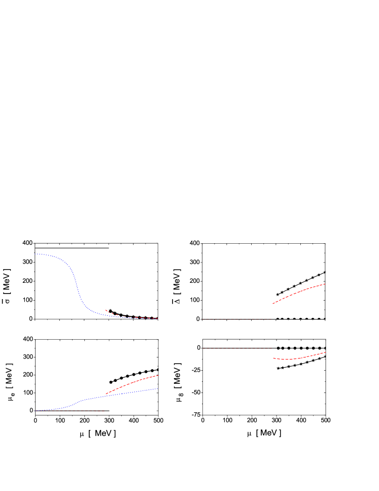
Figure 29: (Color online) Behavior of $\bar{\sigma}$, $\bar{\Delta}$, $\mu_{e}$ and $\mu_{8}$ as functions of the chemical potential, for three different values of the temperature. Solid lines correspond to $T=0$, dashed lines to $T=40$ MeV and dotted lines to $T=100$ MeV. In the case of $T=0$, lines marked with stars and dots correspond to 2SC and NQM phases respectively. The nlNJL model parameters used here are $m_{c}=5.12$ MeV, $\Lambda=827$ MeV and $G_{S}\Lambda_{0}^{2}=18.78$ GomezDumm:2005hy .

The new 2SC-NQM mixed phase is a way in which the constraint of electric neutrality is globally fulfilled: the coexisting phases have opposite electric charges which neutralize eac other, at a common equilibrium pressure. In its simplest realization, this mixed phase is treated within an approximation in which Coulomb and surface energies are neglected Glendenning:1992vb . For color superconducting quark matter this realization of charge neutrality has been considered e.g. in Refs. Neumann:2002jm and Aguilera:2004ag within the NJL model and an instantaneous nonlocal quark model, respectively. On the other hand, notice that color neutrality has been imposed as a local constraint Shovkovy:2003ce ; Reddy:2005 . This is based on the fact that the color Debye screening length is expected to be short and comparable to the inter-particle distance in the regime of interest. As a consequence, the color chemical potential $\mu_{8}$ turns out to be different in the two components of the mixed phase.

When the temperature is increased up to $\sim 20$ MeV, the transition to a mixed phase is no longer favored and the system goes into a pure 2SC phase. As can be seen from the dashed curves in Fig. 29, for $T=40$ MeV this still shows up as a first order phase transition. For even larger temperatures, it is seen that the 2SC phase is no longer present, and the system undergoes a transition from the CSB phase to a normal quark matter (NQM) phase, in which the chiral symmetry is approximately restored and there is no color superconductivity. For $T=100$ MeV this transition occurs as a smooth crossover, as shown by the dotted lines in Fig. 29. The full phase diagram for $G_{D}/G_{S}=0.75$ is displayed in the central panel of Fig. 30. If one moves along the first order transition line from $T=0$ towards higher temperatures, at $T\simeq 50$ MeV a triple point (3P) is reached. At this point the CSB and 2SC phases coexist with a third NQM phase. Finally, if $T$ is still increased, one reaches a critical end point (CEP) where the first order transition from the CSB to the NQM phase becomes a smooth crossover. For comparison, in Fig. 30 the phase diagrams for $G_{D}/G_{S}=0.5$ and $G_{D}/G_{S}=1$ are also shown.

Figure 30: Phase diagrams for $G_{D}/G_{S}=0.5$, 0.75 and 1. Solid and dashed lines indicate first and second order phase transition curves respectively, dotted lines correspond to crossover-like transitions, and dash-dotted lines delimit the gapless 2SC band. Different phases are denoted as NQM (normal quark matter phase), CSB (chiral symmetry broken phase) and 2SC (two-flavor superconducting phase), while the region marked as “Mixed” corresponds to a NQM-2SC mixed phase. CEP and 3P denote the critical end points and triple points, respectively.

Another feature to be discussed is the presence of the so-called gapless 2SC (g2SC) phases. As it is shown in Fig. 30, g2SC phases are favored in a narrow band close to the 2SC$-$NQM phase border. In this region, in addition to the two gapless modes corresponding to the unpaired blue quarks, the presence of flavor asymmetric chemical potentials $\mu_{dc}-\mu_{uc}\neq 0$ gives rise to another two gapless fermionic quasiparticles SH03 . Although the corresponding dispersion relations cannot be derived analytically owing to the nonlocality of the interactions, the border of the g2SC region can be found numerically. This is done by determining whether for some value of the quark momentum $|\vec{p}|$ the imaginary part of some of the poles of the Euclidean quark propagator vanish in the complex $p_{4}$ plane. Although for the cases shown in the figure the g2SC region is given by a narrow band, it appears to be considerable enlarged depending on the model parametrization GomezDumm:2005hy .

The above phase diagrams can be compared with those obtained for isospin symmetric quark matter. In general, it is seen that the 2SC region becomes reduced when one imposes color and electric charge neutrality conditions. This is what one would expect, since the condition of electric charge neutrality leads in general to unequal $u$ and $d$ quark densities, disfavoring the $u$-$d$ pairing. In any case, the effect is found to be relatively small, and the positions of triple points and critical end points, as well as the shapes of critical lines, remain approximately unchanged GomezDumm:2005hy . Qualitatively similar results for isospin symmetric quark matter have been obtained in the context of a chiral two-flavor quark-meson-diquark model in Ref. Braun:2018svj .

5.2 Astrophysical applications

After having analyzed the thermodynamic features of quark matter, it is natural to investigate if such a state can exist in the cores of cold compact stars, where particles appear to be compressed up to densities several times larger than that of nuclear matter ($n_{0}\sim 0.16$ fm^-3). Unfortunately, a consistent relativistic approach to the quark-hadron phase transition, in which hadrons are treated as bound states of quarks, has not been developed up to now. In this situation, hadronic models, as e.g. the Walecka model or the relativistic Dirac-Brueckner-Hartree-Fock (DBHF) approach, have been proposed for the description of the hadronic phase, and quark models have been considered in order to account for the quark matter phase. In particular, several works have employed nonlocal NJL-like schemes to provide an effective theoretical description of quark matter states inside compact stellar cores.

From the observational side, early measurements of the pulsar J0751+1807 and other neutron stars (NS) in X-ray binaries have indicated the existence of large mass compact stars. This has been confirmed by the further observation of the binary pulsars PSR J1614-2230, PSR J0348+0423, PSR J2215+5135 and PSR J0740+6620, with masses of the order of $2\,M_{\odot}$ Demorest:2010bx ; Antoniadis:2013pzd ; Fonseca:2016tux ; Arzoumanian:2017puf ; Linares:2018ppq ; Cromartie:2019kug . The evidence of compact objects of such a large mass can be used as a test for the viability of hadronic and/or quark matter equations of state (EoS) arising from theoretical models Klahn:2006ir . Given the EoS of a neutron star (i.e., the functional relation between pressure and energy density), the corresponding mass vs. radius relation can be obtained through the Tolman-Oppenheimer-Volkoff (TOV) equations of hydrodynamic stability for self-gravitating matter. In general, it is found that a rather stiff EoS is required in order to satisfy observational constraints for large mass neutron stars.

In the context of covariant nonlocal NJL models (instantaneous nlNJL models have been also analyzed, see Ref. Grigorian:2003vi ), the study of a possible quark matter phase in the core of compacts stars has been firstly addressed in Ref. Blaschke:2007ri , considering a two-phase description of the NS interior. In this “hybrid star” scheme, the nuclear matter phase is treated within the relativistic DBHF approach vanDalen:2004pn and the transition to quark matter is obtained through a Maxwell construction. The two-flavor nlNJL model considered in Ref. Blaschke:2007ri includes a diquark coupling of the form proposed in Eq. (131), as well as a current-current vector coupling in the $I=0$ channel, as that in Eq. (66). The presence of a nonvanishing diquark condensate reduces the critical low-temperature transition density (allowing for a quark matter phase in the NS core), whereas the nonzero mean field $\bar{\omega}$ arising from the vector coupling has the effect of stiffening the EoS. This leads to an increase of the maximum accessible NS masses up to a magnitude of about $2M_{\odot}$. The model parameters are similar to those considered in Sec. 5.1 for the study of phase diagrams under compact star conditions, while the proposed additional interaction in the vector channel is relatively weak, and does not affect the qualitative features of the phase transitions Blaschke:2007ri . The numerical results for this model are found to be in agreement with observational constraints for a given range of the model parameters. Moreover, the corresponding isospin symmetric equations of state are shown to be consistent with flow data analyses from heavy ion collisions.

In Refs. Orsaria:2012je ; Orsaria:2013hna the existence of quark matter in the core of NSs has been studied using three-flavor nonlocal NJL models, as those described in Sec. 4. Once again, some repulsive current-current interaction in the $I(J^{P})=0(1^{-})$ channel is included, so as to increase the critical $T=0$ chemical potential and stiffen the quark matter EoS. In turn, the description of the confined, hadronic phase, is carried out by considering the parametrizations GM1 Glendenning:1991es and NL3 Lalazissis:1996rd , within the relativistic mean field theory. The phase regions are determined by assuming a smooth Gibbs transition, in which the condition of pressure equilibrium is imposed together with the requirement of global electric charge neutrality and baryon number conservation Glendenning:1992vb in the mixed quark-hadronic phase. The volume fraction of quark matter is given by a parameter $\chi$, which ranges continuously from 0 to 1 along the transition. Form the corresponding numerical analysis, it is found that the results are compatible with the existence of extended regions of mixed quark-hadron matter in neutron stars with masses of about $2M_{\odot}$ and radii in the canonical range of 12 to 13 km. This holds also for local versions of NJL-like models. Furthermore, it is seen that pure quark matter can exist in stellar cores for certain parametrizations of the effective quark and hadronic interactions. These works have been complemented by the study of the thermal evolution of NSs, obtained from balance and transport equations under the assumption of spherical symmetry deCarvalho:2015lpa . It is found that high-mass NSs may contain a fraction of 35 to 40% of deconfined quark-hybrid matter in their cores, while for stars with canonical masses of around $1.4\,M_{\odot}$ (for which cooling curves show a good agreement with experimental data) a pure hadronic composition is predicted. In this same theoretical context, the possible existence of a crystalline quark-hadron mixed phase and its effects on neutrino emissivity have been studied in Refs. Spinella:2015ksa ; Spinella:2018bdq . Moreover, in Ref. Mellinger:2017dve the existence of quark matter in the cores of rotating NSs has been also considered. On the other hand, in Ref. Ranea-Sandoval:2015ldr it is claimed that if the surface tension at the boundary separating neutral hadronic and neutral quark matter phases is larger than a critical value of about 10 to 40 MeV/fm² Alford:2001zr ; Endo:2011em ; Lugones:2013ema , the mixed phase turns out to be disfavored and there should be a sharp interface between both regions (Maxwell construction). If this is the case, the analysis of Ref. Ranea-Sandoval:2015ldr concludes that large mass hybrid stars would not be allowed within the three-flavor nlNJL approach for quark matter. Similar results are found for the three-flavor local NJL model.

Turning back to astrophysical observations, in the past few years important new constraints for the description of compact stars have come out from the direct detection of gravitational waves emitted from the binary NS merger GW170817 TheLIGOScientific:2017qsa . In particular, the analysis of GW170817 data leads to an upper limit for the tidal deformability —which measures the NS deformation due to the gravitational field of its companion object— and this translates into an upper limit for the NS radius. For a NS mass of 1.4 $M_{\odot}$, it is found that the radius cannot exceed a limit of approximately 13.6 km Raithel:2018ncd . Moreover, it is argued that GW170817 data also imply a general upper limit of about $2.3M_{\odot}$ for the mass of a cold spherical NS Shibata:2019ctb . These constraints have been taken into account for the analysis of EoS arising from hybrid star models that include nlNJL approaches for quark matter Alvarez-Castillo:2018pve ; Ranea-Sandoval:2019miz ; Orsaria:2019ftf ; Malfatti:2019tpg ; Shahrbaf:2019vtf ; Shahrbaf:2020uau ; Malfatti:2020onm .

In Refs. Ranea-Sandoval:2019miz ; Malfatti:2019tpg these new constraints are considered in the context of the above described three-flavor nonlocal NJL models, at both zero and finite temperature. In the finite temperature region, the treatment of quark matter includes the coupling between the quarks and the Polyakov loop, as described in Sec. 2.2. In addition, new parametrizations called DD2 and GM1L are used for the description of the purely hadronic phase. They are based on the standard relativistic mean field approach, taking into account medium effects through the inclusion of explicit density dependent meson-baryon couplings Typel:2009sy ; Ranea-Sandoval:2019miz . The hadron-quark transition is treated according to a Maxwell construction in which there is a sharp interface and no mixed phase regions. For the case of cold neutron stars, it is found that the presence of a quark matter core is allowed for a coupling constant ratio $G_{0}/G_{S}$ lying in a range from $\sim 0.33$ to 0.38 in order to satisfy observational constraints. This is illustrated in Fig. 31, where we show the curves for NS mass vs. radius obtained in Ref. Malfatti:2019tpg after solving the TOV equations, for both GM1L and DD2 hadronic parametrizations. The shaded bands indicate the mass region to be reached in order to fulfill the constraints from the the measurements of PSR J1614-2230 and PSR J0348+0423 masses, while the brown horizontal line indicates the bounds for the radius of a NS star of $M=1.4\,M_{\odot}$ arising from the analysis of GW170817 data. The vertical bars on the curves denote the onset of the transition from hadronic to quark matter. On the other hand, from the study of the evolution of proto-neutron stars to neutron stars it is found that in these models the existence of hybrid stars is allowed only for temperatures not higher than 15 to 30 MeV. Even in the case in which the model parameters are compatible with a quark matter core at $T=0$, this deconfined phase region would disappear for hot neutron or proto-neutron stars. In a more recent work Malfatti:2020onm the analysis has been extended (at $T=0$) to a three-flavor nlNJL model that includes also a 2SC+s superconducting phase. Depending on the stability criteria for the hadron-quark interface, once again it is found that the existence of neutron stars with a superconducting quark matter core can be compatible with observational data. The study of hybrid star constraints has been also carried out in the context of the quark-meson model for quark matter, considering the DD2 parametrization for the hadronic phase Otto:2019zjy .

Figure 31: (Color online) Gravitational mass as a function of the stellar radius for two parametrizations of the hadronic phase. The shaded bands indicate the constraints given by the observed PSR J1614-2230 and PSR J0348+0423 masses, while the horizontal line shows the bounds for a $1.4\,M_{\odot}$ NS radius arising from the analysis of GW170817 data. The vertical bars on the curves denote the onset of the transition from hadronic to quark matter.

Finally, it is worth mentioning that recent works Shahrbaf:2019vtf ; Shahrbaf:2020uau have addressed, in the context of nonlocal NJL-like models, the so-called “hyperon puzzle”. In principle, the core of a NS should include hyperonic degrees of freedom, which soften the EoS in such a way that NS masses larger than $\sim 1.5\,M_{\odot}$ could become unreachable. A possible solution of this puzzle can arise from hybrid NS models, provided that quark deconfinement occurs at low enough densities so as to prevent the existence of hypernuclear matter in the stellar core. In Refs. Shahrbaf:2019vtf ; Shahrbaf:2020uau it is seen that such a scenario can be obtained within two-flavor nlNJL models that include color superconductivity and vector current-current couplings, which lead to a stiff EoS Alvarez-Castillo:2018pve . The hadron-quark phase transition is obtained by a Maxwell construction, considering either fixed or density-dependent couplings. The numerical analysis shows that only in the case of density-dependent couplings an intermediate hypernuclear phase can be found in the cores of hybrid stars. In addition, it is seen that in both situations the onset of deconfinement occurs for compact stars of about 1 to $1.14\,M_{\odot}$. The observational radius and mass constraints are found to be satisfied, circumventing the hyperon puzzle. There are also alternative ways of dealing with this problem, e.g. by considering the effects of three-body forces that involve hyperons, such as nucleon-nucleon-$\Lambda$ interactions. Analyses in this sense have been carried out in Refs. Lonardoni:2014bwa ; Logoteta:2019utx .

5.3 Inhomogenous phases

In the past few years, it has been claimed that the phase diagram of strong-interaction matter at low temperatures and high densities could include spatially nonuniform phases (for a review see e.g. Ref. Buballa:2014tba ). Within the framework of the local two-flavor NJL model in the mean field approximation, it has been shown that the critical end point of the first order chiral restoration transition exactly coincides with the so-called Lifshitz point (LP), where two homogeneous phases and one inhomogeneous phase meet Nickel:2009ke ; Nickel:2009wj . This result has been obtained in the chiral limit, where the critical end point becomes a tricritical point (TCP). If vector-like interactions are added, it is seen that the LP remains at the same temperature, while the TCP moves to a lower $T$, in such a way that it gets covered by the inhomogeneous phase and disappears from the phase diagram Carignano:2010ac . In addition, this issue has been studied in the context of a quark-meson model with vacuum fluctuations Carignano:2014jla , where it is found that the LP might coincide or not with the TCP depending on the model parametrization. In fact, both in the framework of the NJL model and quark-meson models, it is found that the TCP tends to becomes covered by the inhomogeneous phase and does not show up in the phase diagram. The analysis of inhomogeneous phase regions in the context of the Polyakov-NJL model Braun:2015fva and the three-flavor NJL model Carignano:2019ivp , as well as the effects of finite current quark masses Buballa:2018hux , have also been addressed. Moreover, indications of the existence of an inhomogeneous phase have been found in a recent Functional Renormalization Group study of the QCD phase diagram Fu:2019hdw .

In this subsection we discuss the possible presence of inhomogeneous phases in the context of nlNJL models. We consider in particular the analyses in Refs. Carlomagno:2014hoa ; Carlomagno:2015nsa , which correspond to a model similar to the one introduced in Sec. 2.1. Given the complexity of the problem, the derivative currents $j_{R}(x)$ have not been included and the chiral limit $m_{c}=0$ has been taken.

As discussed in Sec. 2.1.1, it is convenient to bosonize the fermionic theory, introducing scalar and pseudoscalar fields that can be expanded around the mean field values $\bar{\sigma}(\vec{x})$ and $\bar{\pi}_{i}(\vec{x})$. These mean field values are now allowed to be inhomogeneous, hence the explicit dependence on spatial coordinates. The resulting mean field Euclidean action reads

$$S^{\rm MFA}_{E}\ =\ -\,\ln\det\ {\cal D}_{0}\;+\;\frac{1}{2G_{S}}\int d^{3}x\;\phi^{a}(\vec{x})\,\phi^{a}(\vec{x})\ ,$$ (133)

where we have defined a chiral four-vector $\phi^{a}=(\bar{\sigma}(\vec{x}),\vec{\bar{\pi}}(\vec{x}))$. In this expression the operator ${\cal D}_{0}$ is given by

$${\cal D}_{0}(x,y)\;=\;\delta^{(4)}(x-y)\;(-i\hbox to0.0pt{/\hss}\partial_{y})\;+\;{\cal G}(x-y)\;\Gamma^{a}\,\phi^{a}\left((\vec{x}+\vec{y})/2\right)\ ,$$ (134)

where $\Gamma^{a}=(1,\vec{\tau})$. The extension to finite temperature $T$ and quark chemical potential $\mu$ can be performed by following the usual Matsubara procedure (see e.g. Sec. 2.2).

The relative locations of the TCP and LP in the $\mu-T$ plane can be studied in general through the so-called Ginzburg-Landau (GL) approach, which does not require to specify the explicit form of the inhomogeneity Nickel:2009ke ; Abuki:2011pf . Following the analysis proposed in Ref. Nickel:2009ke , the mean field thermodynamic potential can be expanded around the symmetric ground state in powers of the order parameters and their spatial gradients. Up to sixth order in this double expansion, the GL functional has the general form Iwata:2012bs

$$\Omega(T,\mu,\phi^{a}(\vec{x})) = \frac{\alpha_{2}}{2}\ \phi^{2}+\frac{\alpha_{4}}{4}(\phi^{2})^{2}+\frac{\alpha_{4b}}{4}(\nabla\phi)^{2}+$$ (135)

$$\frac{\alpha_{6}}{6}(\phi^{2})^{3}+\frac{\alpha_{6b}}{6}(\phi,\nabla\phi)^{2}+\frac{\alpha_{6c}}{6}\left[\phi^{2}(\nabla\phi)^{2}-(\phi,\nabla\phi)^{2}\right]+\frac{\alpha_{6d}}{6}\ (\triangle\phi)^{2}\ ,$$

where $\phi^{2}=(\phi,\phi)=\phi^{a}\phi^{a}=\bar{\sigma}^{2}+\vec{\bar{\pi}}\ \!^{2}$, $(\phi,\nabla_{\!i}\;\phi)=\phi^{a}\nabla_{\!i}\;\phi^{a}=\bar{\sigma}\nabla_{\!i}\;\sigma+\vec{\bar{\pi}}\cdot\nabla_{\!i}\;\vec{\bar{\pi}}$, etc. By looking at this functional, it is seen that for $\alpha_{4b}>0$ the system is in the usual homogeneous phase. Now if in addition one has $\alpha_{4}>0$, the system undergoes a first order chiral restoration transition when $\alpha_{2}=0$ ($\phi^{2}=0$ for $\alpha_{2}>0$, $\phi^{2}\neq 0$ for $\alpha_{2}<0$), which defines a first order transition line in the $\mu-T$ plane. This line ends at the tricritical point, where also $\alpha_{4}=0$ is satisfied. Thus, the position of the TCP can be determined by solving the set of equations

$$\alpha_{2}=0\ ,\qquad\alpha_{4}=0\ .$$ (136)

On the other hand, for $\alpha_{4b}<0$ inhomogeneous solutions are favored. Hence, the Lifshitz point (i.e., the point where the onset of the inhomogeneous phase meets the chiral transition line) is obtained from Buballa:2014tba

$$\alpha_{2}=0\ ,\qquad\alpha_{4b}=0\ .$$ (137)

This general discussion can also be applied to the NJL model, where it can be shown that the coefficients of the quartic terms are equal to each other, i.e. $\alpha_{4}^{\rm NJL}=\alpha_{4b}^{\rm NJL}$ Nickel:2009ke ; Iwata:2012bs ; Carlomagno:2014hoa . Therefore, Eqs. (136) and (137) are simultaneously satisfied, and, as stated above, the TCP and LP are predicted to coincide. This is in general not true in the context of nlNJL models, where the relation becomes modified owing to the presence of the nonlocal form factor Carlomagno:2014hoa . In fact, a numerical analysis carried out in Ref. Carlomagno:2014hoa shows that for various phenomenologically acceptable parametrizations the TCP is located at a higher temperature and a lower chemical potential in comparison with the LP. As a consequence, it is seen that nlNJL models favor a scenario in which the TCP is not covered by the inhomogeneous phase.

Let us investigate, in the framework of nlNJL models, the possible shape of the inhomogeneous phase regions. In principle, a full analysis would require to consider general spatial-dependent condensates, looking for the configurations that minimize the mean field thermodynamic potential at each value of the temperature and chemical potential. Since for an arbitrary 3-dimensional configuration this turns out to be a very difficult task, even in the case of local models it is customary to consider one-dimensional modulations, expecting that the qualitative features of the inhomogeneous phases will not be significantly affected by the specific form of the spatial dependence carried by the condensates Buballa:2014tba . It is worth noticing that, as stated in Ref. Nickel:2009wj , the theoretical problem of finding inhomogeneous phases with a lower dimensional modulation can be reduced to a problem in a lower dimensional theory. Thus, the results from analytically solvable 1+1 dimensional chiral models Schon:2000qy ; Schon:2000he ; Thies:2006ti ; Basar:2009fg ; Bringoltz:2009ym can be used to study the crystalline phase structure in 3+1 dimensions. Here, due to the additional difficulties introduced by the presence of nonlocal quark currents, we consider a simple one-dimensional configuration, namely the so-called dual chiral density wave (DCDW) Nakano:2004cd , in which the chiral condensate rotates along the chiral circle, carrying a constant three-momentum $\vec{Q}$. The spatial dependence of the quark condensates is given in this case by

$$\langle\bar{q}(\vec{x})q(\vec{x})\rangle\ \propto\ \cos(\vec{Q}\cdot\vec{x})\ ,\qquad\qquad\langle\bar{q}(\vec{x})i\gamma_{5}q(\vec{x})\rangle\ \propto\ \sin(\vec{Q}\cdot\vec{x})\ ,$$ (138)

for both $q=u$ and $d$ quark flavors. This behavior of the chiral condensates can be obtained by considering an adequate ansatz for the mean field configuration of the chiral four-vector in momentum space Muller:2013tya .

The values of $\phi$ and $Q\equiv|\vec{Q}|$ can be obtained, as usual, by minimization of the mean field thermodynamic potential $\Omega^{\rm MFA}$. A region in which the absolute minimum is reached for a nonzero $Q$ will correspond to an inhomogeneous phase. As expected, if chiral symmetry is not dynamically broken ($\phi=0$) the regularized thermodynamic potential reduces to the free quark piece $\Omega^{\rm free}_{q}$, which does not depend on $Q$.

Numerical results for the corresponding phase diagrams within nlNJL models have been quoted in Ref. Carlomagno:2015nsa , considering a Gaussian form factor $g(p)=\exp(-p^{2}/\Lambda_{0}^{2})$. Although this analysis does not include the couplings between the quarks and the Polyakov loop, the qualitative features of the phase diagram should not be significantly affected, since one is mostly interested in the low temperature region. In Fig. 32 we quote the results for two parametrizations, which correspond to a pion decay constant $f_{\pi}^{\rm ch}=86$ MeV (we recall that the chiral limit is taken) and quark condensate values $(-\langle\bar{q}q\rangle^{\rm ch})^{1/3}=240$ and 270 MeV, respectively, at zero $T$ and $\mu$. The various regions of the phase diagram, as well as the corresponding transition curves and critical points, are shown in the left panels of Fig. 32. Solid and dashed lines correspond to first and second order transitions, respectively.

Figure 32: (Color online) Left: $\mu-T$ phase diagrams. Solid (dashed) lines indicate first (second) order phase transitions. The dotted line is the lower spinodal corresponding to the homogeneous chiral restoration transition, while the dashed-dotted line is a boundary of a region in which there exists a local inhomogeneous minimum of the thermodynamic potential. TCP, LP and 3P stand for tricritical, Lifshitz and triple points. Right: values of $\phi$ and $Q$ as functions of the chemical potential, for $T=0$.

Let us analyze in detail the phase diagram in the upper left panel, which corresponds to $\langle\bar{q}q\rangle^{\rm ch}=-(240$ MeV$)^{3}$. For low chemical potentials, at temperatures below $\sim 120$ MeV the system lies in an homogeneous chiral symmetry broken (CSB) phase (notice that the corresponding critical temperature should be higher if couplings with the Polyakov loop are included). Taking a fixed temperature of e.g. 100 MeV, by increasing the chemical potential one finds at some critical value $\mu_{c}$($T=100$ MeV) a second order phase transition to an homogeneous normal quark matter (NQM) phase in which chiral symmetry is restored. If the temperature is lowered, the second order transition curve $\mu_{c}(T)$ ends at a tricritical point, beyond which it becomes a first order transition line. Now, by following this line, at a temperature $T_{3P}\simeq 20$ MeV one arrives at a triple point. For $T<T_{3P}$, at a critical chemical potential the system undergoes a first order transition from the CSB phase into an inhomogeneous (IH) phase, in which $Q\neq 0$ and the chiral symmetry is found to be only approximately restored. On the other hand, if one starts with a system in the IH phase and increases the temperature at constant chemical potential, at some critical value of $T$ one arrives at a second order phase transition into the NQM phase. As shown in the figure, the corresponding second order transition line continues beyond the triple point with a dash-dotted line inside the CSB area. The latter is the boundary of a region in which the thermodynamic potential has a local minimum that corresponds to an (unstable) IH phase. Finally, the dotted line in the phase diagram shows the lower spinodal corresponding to the homogeneous chiral restoration transition.

The previously described first order transition from the CSB to the IH phase is illustrated in Fig. 33 Carlomagno:2015nsa . Upper and lower panels show contour plots of the mean field thermodynamic potential at zero temperature for $\mu=260$ and $\mu=280$ MeV, respectively, which correspond to both sides of the transition point $\mu_{c}(0)=274$ MeV. The plots show the transition from an absolute minimum at $\phi\simeq 340$ MeV, $Q=0$, to another one in which $\phi$ reduces to about 50 MeV, while the chiral condensates get spatial dependences as those given by Eq. (138), with $Q\simeq 450$ MeV. These features are also shown in the upper right panel of Fig. 32, where the curves for $\phi$ and $Q$ at $T=0$ as functions of the chemical potential are quoted. Notice that on the CSB side (upper panel of Fig. 33) there also exists a local minimum at $(\phi,Q)\sim(50$ MeV,$\,400$ MeV).

Figure 33: Contour plots of the thermodynamic potential $\Omega^{\rm MFA}$ at zero temperature, close to the first order transition between CSB and IH phases Carlomagno:2015nsa . The plots correspond to a condensate $\langle\bar{q}q\rangle^{\rm ch}=-(240$ MeV$)^{3}$, for chemical potentials $\mu=260$ MeV (up) and $\mu=280$ MeV (down).

If the dimensionless product $G_{S}\Lambda_{0}^{2}$ is decreased, the absolute value of the condensate $|\langle\bar{q}q\rangle^{\rm ch}|$ gets increased, and the onset of the inhomogeneous phase is pushed up to larger values of the chemical potential, leaving a region of homogeneous NQM phase even at $T=0$ Carlomagno:2015nsa . This is shown in the lower left panel of Fig. 32, where we quote the phase diagram for a parameterization leading to $\langle\bar{q}q\rangle^{\rm ch}=-(270$ MeV$)^{3}$ at zero $T$ and $\mu$. In this case, it is seen that the onset of the IH phase (this region is sometimes called a “continent”) occurs at a chemical potential $\mu_{c}(0)$ of the order of 500 MeV. The discontinuity of $Q$ at this transition for $T=0$ becomes increased, as it is shown in the lower right panel of Fig. 32.

It is worth pointing out that for the considered nlNJL models the would-be Lifshitz point appears to be hidden inside the CSB phase region Carlomagno:2015nsa . Instead, a triple point can be found if the CSB and inhomogeneous phases meet. It is also worth mentioning that the second order phase transition curves, as well as both the TCP and would-be LP, can be calculated for these models through a quite precise semianalytical approach GomezDumm:2004sr ; Carlomagno:2014hoa . In addition, it is interesting to notice that, according to the analyses in Refs. Carignano:2011gr ; Carignano:2014jla ; Buballa:2014tba , for both the NJL and quark-meson models some parameterizations lead to phase diagrams that include IH “continents” which extend to arbitrarily high chemical potentials. In fact, it is a matter of discussion whether the emergence of these continents is just a regularization artifact. In nonlocal models the ultraviolet convergence of loop integrals follows from the behavior of form factors, which effectively embrace the underlying QCD interactions (indeed, as discussed in previous sections, the form factors can be fitted from lattice QCD calculations for the effective quark propagators Noguera:2008cm ; Carlomagno:2013ona ; Carlomagno:2019yvi ). The fact that various quark models including different regularization procedures lead to similar qualitative features of the phase diagram seems to indicate that these features are rather robust. However, it is necessary to mention that in the described works the effects of color superconductivity have not been considered. As discussed in Sec. 5.1, the latter are expected to be important at intermediate and large chemical potentials and could have a significant impact on the phase diagram.

5.4 Effects of external strong magnetic fields on phase transitions and meson properties

The study of the behavior of strongly interacting matter under intense external magnetic fields is another subject that has gained significant interest in the past years. Once again, the theoretical analysis requires in general to deal with quantum chromodynamics in nonperturbative regimes, therefore most studies are based either in the predictions of effective models or in the results obtained from lattice QCD calculations. In fact, in view of the theoretical difficulty, most works concentrate on the situations in which one has a uniform and static external magnetic field. Recent reviews on this subject can be found e.g. in Refs. Andersen:2014xxa ; Miransky:2015ava . In this subsection we discuss, in the framework of nonlocal NJL-like models, the features of QCD phase transitions under an intense homogeneous external magnetic field $\vec{B}$ Pagura:2016pwr ; GomezDumm:2017iex . In addition, we show some results on the behavior of $\pi^{0}$ and $\sigma$ meson properties, both at zero and finite temperature GomezDumm:2017jij ; Dumm:2020muy .

At zero temperature, the results of low-energy effective models of QCD as well as LQCD calculations indicate that the size of light quark-antiquark condensates should get increased with the magnetic field. Thus, the external field appears to favor the breakdown of chiral symmetry, which is usually known as “magnetic catalysis”. On the contrary, close to the chiral restoration temperature, LQCD calculations carried out with realistic quark masses Bali:2011qj ; Bali:2012zg show that the condensates behave as nonmonotonic functions of $B$, and this leads to a decrease in the transition temperature when the magnetic field is increased. This effect is known as “inverse magnetic catalysis” (IMC). In addition, LQCD calculations predict an entanglement between the chiral restoration and deconfinement critical temperatures Bali:2011qj . The observation of IMC has become a challenge for effective models. Indeed, most naive effective approaches to low energy QCD predict that the chiral transition temperature should grow with $B$, i.e., they do not find IMC. Interestingly, the corresponding studies carried out in the context of nlNJL models show that the latter are able to describe, at the mean field level, not only the IMC effect but also the entanglement between chiral restoration and deconfinement transition temperatures. Moreover, it is found that the behavior of the mass and decay constant of the $\pi^{0}$ meson as functions of the external magnetic field are also in agreement with LQCD results GomezDumm:2017jij .

Here we concentrate on the two-flavor nlPNJL model introduced in Sec. 2, considering a parametrization of the type of PA, in which quark-antiquark derivative currents are not included. In fact, the general picture is expected to be similar for parametrizations in which such a coupling is also taken into account. To account for the interaction with the magnetic field one can proceed as described in previous sections for the case of axial vector gauge fields. As usual, a coupling between the fermions and the external electromagnetic gauge field $\mathcal{A}_{\mu}$ is obtained by introducing a covariant derivative in the kinetic term in Eq. (1), i.e. by changing

$$\partial_{\mu}\ \rightarrow\ D_{\mu}\equiv\partial_{\mu}-i\,\hat{Q}\mathcal{A}_{\mu}(x)\ ,$$ (139)

where $\hat{Q}=\mbox{diag}(Q_{u},Q_{d})$, with $Q_{u}=2e/3$, $Q_{d}=-e/3$, is the electromagnetic quark charge operator. In addition, as discussed in Sec. 2.1.3, gauge symmetry requires a further change in the nonlocal currents $j_{S}(x)$ and $\vec{\jmath}_{P}(x)$ in Eq. (1), namely

$$\psi(x-z/2)\ \rightarrow\ W_{\rm em}\left(x,x-z/2\right)\;\psi(x-z/2)\ ,$$ (140)

and the corresponding change for $\bar{\psi}(x+z/2)$ Noguera:2008cm . The function $W_{\rm em}({x,y})$ is given by

$$W_{\rm em}(x,y)\ =\ \mathrm{P}\;\exp\left[-\,i\int_{x}^{y}ds_{\mu}\,\hat{Q}\,\mathcal{A}_{\mu}(s)\right]\ ,$$ (141)

where $s$ runs over a path connecting $x$ with $y$. As it is usually done, we take it to be a straight line. As stated, we consider the case of a constant and homogenous magnetic field, which, without loss of generality, can be taken to be orientated along the 3-axis. For definiteness the analysis can be carried out using the Landau gauge, in which one has $\mathcal{A}_{\mu}=B\,x_{1}\,\delta_{\mu 2}$.

As discussed in previous sections, it is convenient to carry out a bosonization of the fermionic theory, introducing scalar and pseudoscalar meson fields and integrating out the fermions. Next, within the mean field approximation, we assume that the scalar field $\sigma$ has a nontrivial translational invariant mean field value $\bar{\sigma}$, while the mean field values of pseudoscalar fields $\vec{\pi}$ are zero. It should be stressed at this point that the assumption stating that $\bar{\sigma}$ is independent of $x$ does not imply that the resulting quark propagator will be translational invariant. In fact, as discussed below, one can show that this invariance is broken by the appearance of the so-called Schwinger phase. Our assumption just states that the deviations from translational invariance driven by the magnetic field are not affected by the dynamics of the theory. In this way, the mean field bosonized action can be written as

$$S^{\rm MFA}_{E}\ =\ -\ln\det\,\mathcal{D}_{0}+V^{(4)}\frac{\bar{\sigma}^{2}}{2G_{S}}\ ,$$ (142)

where

$$\mathcal{D}_{0}(x,x^{\prime})\ =\ {\rm diag}(\mathcal{D}_{0}^{u}(x,x^{\prime})\ ,\ \mathcal{D}_{0}^{d}(x,x^{\prime}))\ ,$$ (143)

with

$$\mathcal{D}_{0}^{f}(x,x^{\prime}) = \ \delta^{(4)}(x-x^{\prime})\left(-i\hbox to0.0pt{/\hss}\partial-Q_{f}B\,x_{1}\gamma_{2}+m_{c}\right)$$ (144)

$$+\;\bar{\sigma}\,{\cal G}(x-x^{\prime})\,\exp\left[i\,\frac{Q_{f}B}{2}(x_{1}+x^{\prime}_{1})\,(x_{2}-x^{\prime}_{2})\right]\,.$$

Here, the function ${\cal G}(z)$ is the nonlocal form factor in the quark currents defined in Eq. (1). Notice that, contrary to the $B=0$ case, in the presence of the magnetic field the charged particles cannot be in states of definite momentum; hence, it is not adequate to transform the action to momentum space. Instead, to deal with the operators $\mathcal{D}_{0}^{f}$ it is convenient to introduce Ritus transforms $\mathcal{D}_{0}^{f}(\bar{p},\bar{p}\,^{\prime})$, defined by

$$\mathcal{D}_{0}^{f}(\bar{p},\bar{p}\,^{\prime})\ =\ \int d^{4}x\ d^{4}x^{\prime}\ \bar{\mathbb{E}}_{\bar{p}}(x)\ \mathcal{D}_{0}^{f}(x,x^{\prime})\ \mathbb{E}_{\bar{p}\,^{\prime}}(x^{\prime})\ ,$$ (145)

where $\mathbb{E}_{\bar{p}}(x)$ and $\bar{\mathbb{E}}_{\bar{p}}(x)$ are Ritus functions Ritus:1978cj . Here $\bar{p}=(k,p_{2},p_{3},p_{4})$, $k$ being an integer quantum number that labels the so-called Landau energy levels. Using the properties of Ritus functions, after some calculation it can be shown that the operators $\mathcal{D}_{0}^{f}$ are diagonal in this basis. One obtains Pagura:2016pwr ; GomezDumm:2017iex

$$\mathcal{D}_{0}^{f}(\bar{p},\bar{p}\,^{\prime})\ =\ (2\pi)^{4}\,\delta_{kk^{\prime}}\,\delta(p_{2}-p_{2}^{\;\prime})\,\delta(p_{3}-p_{3}^{\;\prime})\,\delta(p_{4}-p_{4}^{\;\prime})\ \mathcal{D}^{f}_{k,p_{\parallel}}\ ,$$ (146)

where

$$\mathcal{D}^{f}_{k,p_{\parallel}}\ =\ P_{k,{s_{f}}}\,\Big{(}\!-\!s_{f}\sqrt{2k|Q_{f}B|}\;\gamma_{2}+p_{\parallel}\cdot\gamma_{\parallel}\Big{)}+\sum_{\lambda=\pm}M^{\lambda,f}_{k,p_{\parallel}}\,\Delta^{\lambda}\ ,$$ (147)

with

$$M^{\lambda,f}_{k,p_{\parallel}}\ =\ \frac{4\pi}{|Q_{f}B|}\,(-1)^{k_{\lambda}}\int\frac{d^{2}p_{\perp}}{(2\pi)^{2}}\ \left[m_{c}+\bar{\sigma}\ g(p)\right]\,\exp(-p_{\perp}^{2}/|Q_{f}B|)\,L_{k_{\lambda}}(2p_{\perp}^{2}/|Q_{f}B|)\ .$$ (148)

In these equations the definitions $s_{f}={{\rm sgn}}(Q_{f}B)$, $p_{\parallel}=(p_{3},p_{4})$, $p_{\perp}=(p_{1},p_{2})$, $\gamma_{\parallel}=(\gamma_{3},\gamma_{4})$, $\Delta^{+}=\mbox{diag}(1,0,1,0)$, $\Delta^{-}=\mbox{diag}(0,1,0,1)$, $P_{k,\pm 1}=(1-\delta_{k0})\,{I}+\delta_{k0}\,\Delta^{\pm}$ and $k_{\pm}=k-1/2\pm s_{f}/2\,$ have been used. The function $g(p)$ stands for the Fourier transform of ${\cal G}(x)$, while $L_{m}(x)$ are Laguerre polynomials, with the usual convention $L_{-1}(x)=0$.

Using the fact that $\mathcal{D}_{0}^{f}$ is diagonal in Ritus space, the corresponding contribution to the mean field action can be readily calculated. One obtains

$$\frac{S^{\rm MFA}_{E}}{V^{(4)}}\ =\ -N_{c}\sum_{f=u,d}\frac{|Q_{f}B|}{2\pi}\int\frac{d^{2}p_{\parallel}}{(2\pi)^{2}}\bigg{[}\ln\left(p_{\parallel}^{2}+{M^{\,\lambda_{\!f},f}_{0,p_{\parallel}}\,}^{2}\,\right)+\sum_{k=1}^{\infty}\ \ln\Delta^{f}_{k,p_{\parallel}}\bigg{]}+\frac{\bar{\sigma}^{2}}{2G}\ ,$$ (149)

where $\lambda_{f}=+\,(-)$ for $s_{f}=+1\,(-1)$, and $\Delta^{f}_{k,p_{\parallel}}$ is defined by

$$\Delta^{f}_{k,p_{\parallel}}\ =\ \left(2k|Q_{f}B|+p_{\parallel}^{2}+M^{+,f}_{k,p_{\parallel}}\,M^{-,f}_{k,p_{\parallel}}\right)^{2}+p_{\parallel}^{2}\left(M^{+,f}_{k,p_{\parallel}}-M^{-,f}_{k,p_{\parallel}}\right)^{2}\ .$$ (150)

By regarding at these equations [compare with Eq. (10)] it is seen that the functions $M^{\pm,f}_{k,p_{\parallel}}$ play the role of constituent quark masses in the presence of the external magnetic field.

As done in Sec. 2.2, the analysis can be extended to a system at finite temperature using the Matsubara formalism, and a coupling of fermions to the Polyakov loop can be included to account for confinement effects. In what follows we present the results corresponding to the polynomial PL potential quoted in Eq. (32) Ratti:2005jh . The full expression of the corresponding mean field thermodynamic potential can be found in Ref. GomezDumm:2017iex . As in the $B=0$ case, this quantity is divergent and can be regularized using the prescription in which one subtracts a free contribution and adds it in a regularized form. In fact, this “free” contribution corresponds to the mean field potential obtained in absence of the effective four-quark coupling (i.e. setting $\bar{\sigma}=0$), but keeping the interaction with the magnetic field and the PL.

By minimizing the regularized mean field thermodynamic potential one can obtain the values of $\bar{\sigma}$ and the traced Polyakov loop $\Phi$ as functions of the temperature $T$ and the magnetic field. Then, the magnetic field dependent quark condensates $\langle\bar{q}q\rangle$, $q=u,d$, can be calculated, as usual, by taking the derivatives with respect to the corresponding current quark masses. To make contact with LQCD results given in Ref. Bali:2012zg it is convenient to define the quantities

$$\Sigma^{q}_{B,T}\ =\ -\frac{2\,m_{c}}{S^{4}}\,\Big{[}\langle\bar{q}q\rangle_{B,T}-\langle\bar{q}q\rangle_{0,0}\Big{]}\,+\,1\ ,$$ (151)

where $S=(135\times 86)^{1/2}$ MeV. We also introduce the definitions $\Delta\Sigma^{q}_{B,T}=\Sigma^{q}_{B,T}-\Sigma^{q}_{0,T}$, $\bar{\Sigma}_{B,T}=(\Sigma^{u}_{B,T}+\Sigma^{d}_{B,T})/2$ and $\Delta\bar{\Sigma}_{B,T}=(\Delta\Sigma^{u}_{B,T}+\Delta\Sigma^{d}_{B,T})/2\,$, which correspond to a subtracted normalized flavor condensate, a normalized flavor average condensate and a subtracted normalized flavor average condensate, respectively.

In what follows we quote the numerical results obtained for the case of a Gaussian form factor, i.e. for some parametrizations similar to PA (see Sec. 2.3). For comparison we consider parameter sets leading to quark-antiquark condensates $(-\langle\bar{q}q\rangle_{0,0})^{1/3}=240$, 230 and 220 MeV. The corresponding model parameters can be found e.g. in Ref. GomezDumm:2017iex .

The behavior of quark condensates at zero temperature within this nlNJL framework has been calculated in Ref. Pagura:2016pwr . The results are shown in Fig. 34, where we include the predictions for $\Delta\bar{\Sigma}_{B,0}$ and $\Sigma^{u}_{B,0}-\Sigma^{d}_{B,0}$ as functions of $eB$ together with the corresponding LQCD data given in Ref. Bali:2012zg . Solid, dashed and dotted curves correspond to $(-\langle\bar{q}q\rangle_{0,0})^{1/3}=240$, 230 and 220 MeV, respectively. The growth of the condensates clearly show the effect known as “magnetic catalysis”. It can be seen that the predictions for $\Delta\bar{\Sigma}_{B,0}$ are very similar for all parameter sets, while for the difference $\Sigma^{u}_{B,0}-\Sigma^{d}_{B,0}$ there is some dependence on the parametrization. In both cases the predictions show a good agreement with LQCD results.

Figure 34: (Color online) Normalized quark condensates as functions of the magnetic field at $T=0$. Solid (blue), dashed (black) and dotted (red) curves correspond to parameterizations leading to $(-\langle\bar{q}q\rangle_{0,0})^{1/3}=240$, 230 and 220 MeV, respectively. Full square symbols indicate LQCD results given in Ref. Bali:2012zg .

Let us now look at the results for a system at finite temperature, which have been obtained in Ref. GomezDumm:2017iex . In the left panel of Fig. 35 we show the behavior of the averaged chiral condensate $\bar{\Sigma}_{B,T}$ and the traced Polyakov loop $\Phi$ as functions of the temperature, for three representative values of the external magnetic field, namely $eB=0$, 0.6 and 1 GeV². The curves correspond to a quark condensate $(-\langle\bar{q}q\rangle_{0,0})^{1/3}=230$ MeV. Given a value of $B$, it is seen from the figure that chiral restoration and deconfinement transitions proceed as smooth crossovers occurring at approximately the same critical temperature $T_{c}(B)$ (chiral restoration and deconfinement critical temperatures are defined here from the peaks in the derivatives $-d\bar{\Sigma}_{B,T}/dT$ and $d\Phi/dT$, respectively). For $B=0$, $T_{c}(0)$ is found to be approximately equal to 180 MeV, with a variation not larger than a few percent within the above considered parametrization range. This temperature compares well with the value $T_{c}(0)=173\pm 8$ MeV obtained from $N_{f}=2$ LQCD calculations Karsch:2003jg . It is worth recalling that in absence of the interaction with the Polyakov loop the value of $T_{c}(0)$ is found to drop down to about 130 MeV Pagura:2016pwr .

(a)

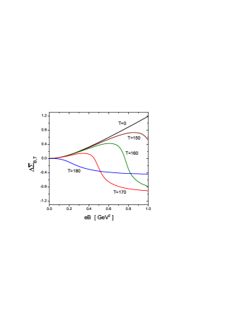
(b)

Figure 35: (Color online) Left: normalized flavor average condensate and traced Polyakov loop as functions of the temperature, for three representative values of $eB$. Right: subtracted normalized flavor average condensate as a function of $eB$ for various representative temperatures.

It is interesting to discuss the effect of the magnetic field on the phase transition features. On one hand, from the left panel of Fig. 35 it is seen that the splitting between the chiral restoration and deconfinement critical temperatures remains very small even for nonzero $B$. On the other hand, the curves for the normalized flavor average condensate clearly show the inverse magnetic catalysis effect. Indeed, contrary to what happens e.g. in the local NJL model Andersen:2014xxa ; Miransky:2015ava or in the quark-meson model Fraga:2013ova , within the nlNJL approach the chiral restoration critical temperature becomes lower as the external magnetic field is increased. This is related with the fact that the condensates do not show in general a monotonic increase with $B$ for a fixed value of the temperature. The situation is illustrated in the right panel of Fig. 35, where we show the behavior of the averaged difference $\Delta\bar{\Sigma}_{B,T}$ as a function of $eB$, for $T=0$ and for values of the temperature in the critical region. While the value of $\Delta\bar{\Sigma}_{B,T=0}$ shows a monotonic growth with the external magnetic field, it is seen that when the temperatures get closer to critical values $T_{c}(B)$ the curves show a maximum and then start to decrease for increasing $B$. This is a typical behavior associated to IMC and nicely agrees with the results obtained from lattice QCD, see e.g. Fig. 2 of Ref. Bali:2012zg .

In Fig. 36 we show the results given in Ref. GomezDumm:2017iex for the normalized chiral restoration critical temperature, $T_{c}(B)/T_{c}(0)$, as a function of $eB$. The curves correspond to the above mentioned nlNJL model parametrizations. For comparison, LQCD results quoted in Ref. Bali:2012zg are indicated by the gray band. From the figure it is clearly seen that the IMC effect is sizeable, and fully compatible with LQCD results for phenomenologically adequate values of the chiral condensate. It is also worth mentioning that some effective approaches to low energy QCD are able to obtain IMC by assuming some explicit dependence of the effective coupling parameters on $B$ and/or $T$ Ayala:2014iba ; Farias:2014eca , or by considering the effect of anomalous magnetic moments in the quark energy dispersion relations Fayazbakhsh:2014mca . In turn, it is seen that within nlNJL models one gets IMC in a fully natural way. This can be understood by noticing that for a given Landau level the associated nonlocal form factor carries a dependence on the external magnetic field, which arises from the convolution in Eq. (148).

Figure 36: (Color online) Normalized critical temperatures as functions of $eB$. For comparison, LQCD results of Ref. Bali:2012zg are indicated by the gray band.

In what follows we quote some results concerning the properties of the $\pi^{0}$ meson in the presence of the external magnetic field. At zero temperature, the theoretical expression for the $\pi^{0}$ mass can be obtained by expanding the corresponding bosonic action in powers of the fluctuations $\delta\pi_{3}=\delta\pi^{0}$. In momentum space the corresponding quadratic piece of the bosonized action can be written as

$$S^{\rm quad}_{E}\Big{|}_{(\delta\pi^{0})^{2}} = \frac{1}{2}\int\frac{d^{4}q}{(2\pi)^{4}}\ G_{\pi^{0}}(q_{\perp}^{2},q_{\parallel}^{2})\ \delta\pi^{0}(q)\,\delta\pi^{0}(-q)$$ (152)

$$= \frac{1}{2}\int\frac{d^{4}q}{(2\pi)^{4}}\ \left[\frac{1}{G_{S}}\,+F_{\pi^{0}}(q_{\perp}^{2},q_{\parallel}^{2})\right]\,\delta\pi^{0}(q)\,\delta\pi^{0}(-q)\ ,$$

where the polarization function $F_{\pi^{0}}(q_{\perp}^{2},q_{\parallel}^{2})$ is given by a quark loop integral that involves the external field $B$. Its explicit form can be found in Refs. GomezDumm:2017jij ; Dumm:2020muy . Choosing the frame in which the pion is at rest, its mass can be obtained as a solution of the equation

$$G_{\pi^{0}}(0,-m_{\pi^{0}}^{2})=\ 0\ .$$ (153)

As shown in Ref. Fayazbakhsh:2013cha , a relevant feature induced by the presence of the external magnetic field is the fact that the $\pi^{0}$ dispersion relation turns out to be anisotropic, implying that the movement along the direction perpendicular to the magnetic field is characterized by a directional refraction index $u_{\pi^{0}}$ which is in general different from one. To normalize the $\pi^{0}$ field one can expand the action in Eq. (152) around the pion pole ($q_{\perp}=0$, $q_{\parallel}^{2}=-m_{\pi^{0}}^{2}$) up to first order in momentum squared. Following Ref. Dumm:2020muy one can define

$$Z_{\parallel}^{-1}\ =\ g_{\pi^{0}q\bar{q}}^{-2}\ =\ \dfrac{dG_{\pi^{0}}(q_{\perp}^{2},q_{\parallel}^{2})}{dq_{\parallel}^{2}}\bigg{\rvert}_{q_{\perp}^{2}=0,\,q_{\parallel}^{2}=-m_{\pi^{0}}^{2}},\qquad Z_{\perp}^{-1}\ =\ \dfrac{dG_{\pi^{0}}(q_{\perp}^{2},q_{\parallel}^{2})}{dq_{\perp}^{2}}\bigg{\rvert}_{q_{\perp}^{2}=0,\,q_{\parallel}^{2}=-m_{\pi^{0}}^{2}}\ ,$$ (154)

renormalizing the pion field according to $\pi^{0}(q)=Z_{\parallel}^{1/2}\,\tilde{\pi}^{0}(q)$. Thus, around the pion pole one has

$$S_{E}^{\rm quad}\Big{|}_{(\delta\pi^{0})^{2}}\ =\ \dfrac{1}{2}\int\frac{d^{4}q}{(2\pi)^{4}}\,\Big{(}u_{\pi^{0}}^{2}\,q_{\perp}^{2}+q_{\parallel}^{2}+m_{\pi^{0}}^{2}\Big{)}\,\delta\tilde{\pi}^{0}(q)\delta\tilde{\pi}^{0}(-q)\ ,$$ (155)

where

$$u_{\pi^{0}}^{2}\ =\ \dfrac{Z_{\parallel}}{Z_{\perp}}\ .$$ (156)

The behavior of the pion mass $m_{\pi^{0}}(B)$ predicted by the nlNJL approach is shown in Fig. 37 GomezDumm:2017jij . The results, normalized to the empirical $\pi^{0}$ mass value at $B=0$, correspond to the parameter set leading to $(-\langle\bar{q}q\rangle_{0,0})^{1/3}=230$ MeV. It is found that the $\pi^{0}$ mass decreases when the magnetic field gets increased, reaching a value of about 65% of $m_{\pi^{0}}(0)$ at $eB\simeq 1.5$ GeV², which corresponds to a magnetic field of about $2.5\times 10^{20}$ G. The figure also includes a gray band that corresponds to lattice QCD results given in Ref. Bali:2017ian . The latter have been obtained from a continuum extrapolation of lattice spacing, considering a relatively large current quark mass for which $m_{\pi}=415$ MeV. For comparison, we also quote in the figure the results obtained within the nlNJL model by shifting $m_{c}$ to 56.3 MeV, which leads to this enhanced pion mass. In general, it can be seen that nlNJL model predictions —for which no ad-hoc adjustments or extra parameters have been required— turn out to be in good agreement with LQCD calculations. It is also worth mentioning that the curves in Fig. 37 remain practically unchanged when the value of the $B=0$ condensate used to fix the parametrization is varied within the range from $-$(220 MeV)³ to $-$(250 MeV)³.

Figure 37: Mass of the $\pi^{0}$ meson as a function of $eB$, normalized to its value for $B=0$ GomezDumm:2017jij . The dotted line is obtained for a parameterization in which $m_{\pi}=415$ MeV, while the gray band corresponds to the results of lattice QCD calculations quoted in Ref. Bali:2017ian .

It is also interesting to study the behavior of the $\pi^{0}$ meson “decay constants”. As shown in Ref. Coppola:2018ygv , in the presence of an external magnetic field $\vec{B}$ the pion-to-vacuum vector and axial vector amplitudes can be in general parameterized in terms of three form factors. Two of them, $f_{\pi^{0}}^{(A||)}$ and $f_{\pi^{0}}^{(A\perp)}$, in the $B=0$ limit reduce to the pion decay constant usually denoted by $f_{\pi}$. The third one, $f_{\pi^{0}}^{(V)}$, is associated to the vector piece of the quark weak current, and vanishes for $B=0$. Following the notation in Ref. Coppola:2019uyr , these form factors can be defined by the relations

$$H_{4}^{V}(x,\vec{q})\pm H_{3}^{V}(x,\vec{q}) = \mp\,f^{(V)}_{\pi^{0}}(q_{4}\mp q_{3})\,e^{iq\,\cdot x}\ ,$$

$$H_{1}^{V}(x,\vec{q})\pm iH_{2}^{V}(x,\vec{q}) = 0\ ,$$

$$H_{4}^{A}(x,\vec{q})\pm H_{3}^{A}(x,\vec{q}) = -if^{(A\parallel)}_{\pi^{0}}(q_{4}\pm q_{3})\,e^{iq\,\cdot x}\ ,$$

$$H_{1}^{A}(x,\vec{q})\pm iH_{2}^{A}(x,\vec{q}) = -if^{(A\perp)}_{\pi^{0}}(q_{1}\pm iq_{2})\,e^{iq\,\cdot x}\ ,$$ (157)

where $H_{\mu}^{V,A}$ are the $\pi^{0}$-to-vacuum amplitudes for vector and axial vector quark currents,

$$H_{\mu}^{V}(x,\vec{q}) = \langle 0|\bar{\psi}(x)\,\gamma_{\mu}\frac{\tau^{3}}{2}\,\psi(x)|\tilde{\pi}^{0}(\vec{q})\rangle\ ,$$

$$H_{\mu}^{A}(x,\vec{q}) = \langle 0|\bar{\psi}(x)\,\gamma_{\mu}\gamma_{5}\frac{\tau^{3}}{2}\,\psi(x)|\tilde{\pi}^{0}(\vec{q})\rangle\ .$$ (158)

The matrix elements in Eq. (158) can be obtained by introducing couplings between the quark currents and auxiliary vector and axial vector gauge fields, and then taking the corresponding functional derivatives of the effective action. Once again, gauge invariance requires the couplings to these auxiliary gauge fields to be introduced through the covariant derivative and the parallel transport of the fermion fields. The analytic calculations of the form factors require to carry out combined Laguerre-Fourier transformations of the form factors. Explicit expressions can be found in Ref. Dumm:2020muy .

It is interesting to study the relations involving form factors and renormalization constants in the chiral limit, $m_{c}\to 0$. As expected, in this limit one gets ${F_{\pi^{0}}(0,0)}=-1/G_{S}$ Dumm:2020muy , which implies $m_{\pi^{0}}=0$ according to Eq. (153). In addition, from the calculations in Refs. GomezDumm:2017jij ; Dumm:2020muy it is seen that the Goldberger-Treiman relation

$$f_{\pi^{0},0}^{(A\parallel)}\;Z_{\parallel,0}^{1/2}\ =\ \bar{\sigma}_{0}$$ (159)

and the Gell-Mann-Oakes-Renner relation

$${f_{\pi^{0},0}^{(A\parallel)}}^{2}\,m_{\pi^{0}}^{2}\ =\ -\,m_{c}\,\langle\bar{u}u+\bar{d}d\rangle_{0}$$ (160)

remain valid in the presence of the external magnetic field (subindices 0 indicate that the involved quantities are evaluated in the chiral limit). The above equations are complemented by the relation Dumm:2020muy

$$f_{\pi^{0},0}^{(A\perp)}\,Z_{\parallel,0}^{-1/2}\,Z_{\perp,0}\ =\ \bar{\sigma}_{0}\ ,$$ (161)

which implies

$$\frac{f_{\pi^{0},0}^{(A\perp)}}{f_{\pi^{0},0}^{(A\parallel)}}\ =\ \frac{Z_{\parallel,0}}{Z_{\perp,0}}\ =\ u_{\pi^{0},0}^{2}\ .$$ (162)

This result has been also found in the framework of the local NJL model in Ref. Coppola:2019uyr , and (using a different notation) in Ref. Fayazbakhsh:2013cha , where it is obtained from a modified partially-conserved-axial-current (PCAC) relation.

In Fig. 38 we show the numerical results obtained within the nlNJL model for various quantities associated with the neutral pion at zero temperature, as functions of $eB$ Dumm:2020muy . Dashed, solid and dotted red lines correspond to quark condensate values $(-\langle\bar{q}q\rangle_{0,0})^{1/3}=220$, 230 and 240 MeV, respectively. For comparison we also include in the figure the numerical results obtained within the local NJL model, quoted in Ref. Coppola:2019uyr . Solid blue lines correspond to a parametrization leading to a constituent quark mass $M=350$ MeV (for $B=0$), while the limits of the gray bands correspond to $M=320$ MeV (dashed lines) and $M=380$ MeV (dotted lines). The values of the $B=0$ quark-antiquark condensates for these parametrizations of the NJL model are $\langle\bar{q}q\rangle\simeq(-243~{}\rm{MeV})^{3}$, $(-236~{}\rm{MeV})^{3}$ and $(-250~{}\rm{MeV})^{3}$, respectively. As shown in the figure, in general nlNJL results do not show a large dependence with the model parametrization. On the other hand, in most cases the dependence with the external field is significantly stronger for the nlNJL model than for the local NJL approach. In the case of the effective coupling constant $g_{\pi^{0}q\bar{q}}$, the behavior is found to be opposite for both models. Concerning the axial form factors, for $B=0$ one has spacial rotation symmetry and both $f_{\pi^{0}}^{(A\parallel)}$ and $f_{\pi^{0}}^{(A\perp)}$ reduce to the usual pion decay constant $f_{\pi}$ [see Eqs. (158)]. As the magnetic field increases, $f_{\pi^{0}}^{(A\parallel)}$ gets enhanced and $f_{\pi^{0}}^{(A\perp)}$ gets reduced, both in the case of the nlNJL and the local NJL model. The vector form factor $f_{\pi^{0}}^{(V)}$, shown in the lower left panel, is zero at vanishing external field and shows a monotonic growth with $eB$, with little dependence on the parametrization within the nlNJL model.

Figure 38: (Color online) Neutral pion properties as functions of $eB$. Solid red and blue lines correspond nlNJL and local NJL results, respectively. The gray bands account for model parameter ranges indicated in the text.

Finally, let us discuss the behavior of $\pi^{0}$ and $\sigma$ meson properties in the context of nlNJL models for a system at finite temperature $T$. As in the case of the quark condensates, we quote the results for the model parametrization corresponding to $(-\langle\bar{q}q\rangle_{0,0})^{1/3}=230$ MeV and a polynomial PL potential. In Fig. 39 we show the behavior of the $\pi^{0}$ and $\sigma$ meson masses (upper panel), and the normalized $\pi^{0}$ axial and vector decay form factors (lower panel) as functions of the temperature, for three representative values of the external magnetic field, namely $eB=0$, $eB=0.6$ GeV² and $eB=1$ GeV². These results have been obtained in Ref. Dumm:2020muy . It can be seen that for nonzero $B$ the masses show a similar qualitative behavior with $T$ as in the $B=0$ case. The $\pi^{0}$ mass remains approximately constant up to the critical temperature, and $\pi^{0}$ and $\sigma$ masses match above $T_{c}(B)$, as expected from chiral symmetry. For large temperatures it is seen that the masses get steadily increased, the growth being dominated by pure thermal effects. As stated, the IMC effect is observed, i.e., $T_{c}(B)$ gets lower for increasing $B$. In the case of the form factors, the curves for $f_{\pi^{0}}^{(A\parallel)}$ and $f_{\pi^{0}}^{(V)}$ show sudden drops at the critical temperatures, exhibiting once again a qualitatively similar behavior for zero and nonzero external magnetic field. The curves for $f_{\pi^{0}}^{(A\perp)}$ overlap with those corresponding to $f_{\pi^{0}}^{(A\parallel)}$ and are not displayed in the figure. We recall that, at any temperature, $f_{\pi^{0}}^{(V)}$ is zero for vanishing external field.

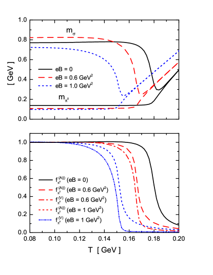
Figure 39: (Color online) $\pi^{0}$ and $\sigma$ meson masses (upper panel) and normalized $\pi^{0}$ decay form factors (lower panel) as functions of the temperature, for three representative values of $eB$.

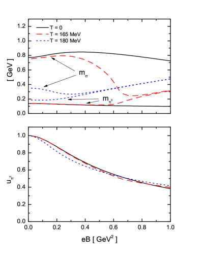
(a)

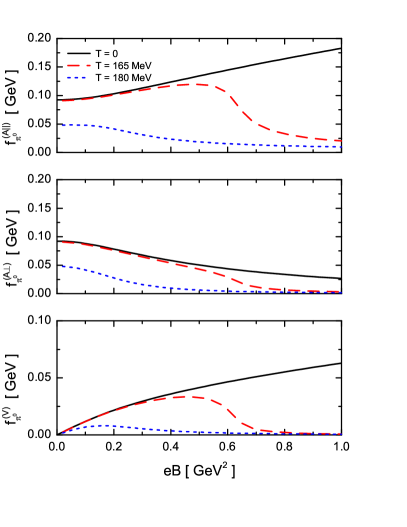
(b)

Figure 40: (Color online) Left: $\pi^{0}$ and $\sigma$ meson masses and directional refraction index as functions of $eB$, for three representative values of the temperature. Right: from top to bottom, decay form factors $f_{\pi^{0}}^{(A\parallel)}$, $f_{\pi^{0}}^{(A\perp)}$ and $f_{\pi^{0}}^{(V)}$ as functions of $eB$, for three representative values of the temperature.

For completeness, in Fig. 40 we show the behavior of meson properties as functions of $eB$ for three representative values of the temperature, namely $T=0$, 165 MeV and 180 MeV Dumm:2020muy . The results for $T=0$, same as those previously shown in Fig. 39, are included just for comparison. The curves for $T=165$ MeV can be understood by looking at the results in Fig. 35, which show that this is the critical temperature that corresponds to $eB\simeq 0.6$ GeV². Thus, for this temperature, the pion mass and form factors in Fig. 40 are expected to show approximately the same behavior as for $T=0$ up to $eB\sim 0.5-0.6$ GeV². Beyond these values, as expected from the results in Fig. 39, one finds an enhancement of the pion mass and a decrease of the axial and vector form factors. On the other hand, it is seen that for $T=180$ MeV the values of the pion mass and axial form factors are well separated from the $T=0$ values already at $B=0$. This reflects the fact that at $T\sim 180$ MeV the system is undergoing the chiral restoration transition for vanishing magnetic field.

6 Summary & concluding remarks

In this work we have presented an overview of the current status of the research on effective nonlocal NJL-like chiral quark models. Within this framework, we have analyzed the description of hadron properties in vacuum, as well as the features of deconfinement and chiral restoration transitions for systems at finite temperature and/or density. In addition, we have addressed other related subjects, such as the study of phase transitions for imaginary chemical potentials, the possible existence of inhomogeneous phase regions, the presence of color superconductivity, the effects produced by strong external magnetic fields and the applications to the description of compact stellar objects.

The reliability of nlNJL models and their advantage over the standard, local NJL model can be evaluated by comparing the obtained predictions against vacuum hadron phenomenology and existing results from lattice calculations, in particular, in the region of low or vanishing chemical potentials. Here, we have started by considering a two-flavor model (see Sec. 2), which has been extended by including interaction channels that account for vector and axial vector meson physics (Sec. 3). Then, the extension to three flavors has been also reviewed (Sec. 4). In all these approaches the underlying QCD interactions are effectively taken into account through a few coupling constants and nonlocal form factors. In the simplest versions of the nonlocal NJL-like models (see Sec. 2), these form factors can be obtained from a fit to lattice QCD results for the momentum dependence of effective quark propagators. In fact, a general analyses of the results presented throughout this article shows that most qualitative predictions of nlNJL models do not depend significantly on the ultraviolet behavior of the form factors. Hence, in many cases it is convenient to use Gaussian functions, which guarantee a rapid convergence of quark loop integrals and simplify analytical calculations. It is also shown that —as expected— a more accurate fit to LQCD results for quark propagators leads to a better agreement between nlNJL model and LQCD predictions for thermodynamical quantities (see Sec. 4). After determining the values of the coupling constants from a few input empirical quantities, various particle properties can be obtained as predictions of the models. As shown by Tables 2, 6 and 10, these results show in general a reasonable agreement with the observed phenomenology. This includes both the $J=1$ and the strange meson sectors. On the other hand, there is a good agreement with most lattice QCD results for finite temperature and low chemical potentials, and also for the theoretical case of imaginary chemical potentials. A point that deserves further investigation is the thermal behavior of the traced Polyakov loop, for which the comparison between quark effective models and LQCD data has to be taken with some care (see discussion in Sec. 4.4).

Concerning the comparison with standard local NJL-like approaches, there are several reasons for which nonlocal models are expected to be more adequate for the description of low energy QCD phenomenology than local effective theories. In fact, as stated in Sec. 2, nonlocality arises naturally in the context of various successful approaches to strong interactions in the nonperturbative regime, covering from the instanton liquid model to Dyson-Schwinger resummation methods. Moreover, the presence of well behaved form factors in nonlocal models ensures the convergence of quark loop integrals, which make nlNJL predictions more stable against changes in model parameters in comparison with models that include sharp cutoff regularizations. At the same time, the assumption of a separable interaction makes these nlNJL-like schemes capable of retaining much of the simplicity of the local NJL model, in comparison with more rigorous analytical approaches to nonperturbative QCD. While for many physical quantities the results are similar for both local and nonlocal approaches, there are some cases in which significant qualitative differences show up. One of them is the entanglement between chiral restoration and deconfinement critical temperatures. This feature is observed from LQCD results and arises naturally in the framework of nlPNJL models (see Secs. 2.4 and 4.4), while local models predict in general a splitting between critical temperatures. Another example is the dependence of the pion decay constant, $f_{\pi}$, on the value of the explicit chiral symmetry breaking parameter $m_{c}$ (or, equivalently, on the pion mass). As shown in Fig. 4 (right panel), the results from nlNJL models show a much better agreement with LQCD results than those obtained within local NJL schemes. In addition, special attention should be deserved to the effects of an external strong magnetic field on phase transitions and meson properties. As shown in Sec. 5.4, nlNJL models predict the existence of inverse magnetic catalysis, according to which the chiral restoration transition temperature behaves as a decreasing function of the external magnetic field. It is worth pointing out that this effect, which has been found by LQCD calculations, arises naturally in the context of nlNJL approaches due to the magnetic field dependence of nonlocal form factors. In the local NJL the inverse magnetic catalysis can be obtained only after the inclusion of some ad-hoc mechanism, such as e.g. the assumption of an explicit dependence of the coupling constants on the magnetic field. With no ad-hoc adjustments, a good agreement between nlNJL models and lattice QCD results for the behavior of critical temperatures is found, as shown in Fig. 36. Moreover, the predictions of nlNJL models for the behavior of the $\pi^{0}$ mass as a function of the magnetic field also show excellent agreement with LQCD data, as shown in Fig. 37. It is seen that, in general, there are significant differences between local and nonlocal model predictions for the magnetic field dependence of various $\pi^{0}$ properties (see Fig. 38).

We also find it important to state some remarks on $\mu-T$ phase diagrams. For almost all studied parametrizations, nonlocal models predict the existence of a critical end point separating crossover-like and first order transition critical temperatures. This is in accordance with the general belief from most approaches to effective models for low energy strong interactions. From the phase diagrams in Figs. 8, 17 and 26 it can be seen that, in general, the CEP location is found to lie within a range of temperatures between 120 and 170 MeV and (quark) chemical potentials from 150 to 250 MeV. The precise position depends on the model parametrization and the form of the Polyakov loop potential, which accounts for confinement features and is a major source of uncertainty for both local and nonlocal NJL-like approaches. It is worth remarking that, as discussed in Secs. 5.1 and 5.3, nlNJL models allow for the presence of two-flavor superconducting states and mixed phases, as well as inhomogeneous phase regions. In particular, as discussed in Sec. 5.2, several works show that the existence of mixed and/or quark matter phases in the deep core of compact stars is compatible with present observational constraints. Regarding inhomogeneous (or crystalline) phases, it is worth mentioning that local two-flavor NJL models predict the existence of a so-called Lifshitz point —which in the chiral limit coincides with the tricritical point— whereas in the nlNJL models studied here the would-be Lifshitz point appears to be hidden into the hadronic phase in which chiral symmetry is spontaneously broken (see Fig. 32). Depending on the parametrization, one can find instead a triple point, in which hadronic, quark matter and inhomogeneous phases meet.

As a general conclusion, it could be stated that nonlocal NJL-like models provide a scenario in which several of the traditional problems of the NJL model are overcome, whilst much of the simplicity and predictive power of the standard local approach is retained. Moreover, the general good agreement with lattice QCD results for both zero and finite temperature indicates that the nlNJL model approach serves as a successful tool to deal with the description of nonperturbative QCD features, and can be used to get predictions for the behavior of hadronic and quark matter systems at finite densities and/or in the presence of external fields.

Appendix: Basic notation and conventions

Throughout this article we use Euclidean space-time coordinates $x_{\mu}=(\vec{x},x_{4})$, where $x_{4}=ix_{0}$. Then, the associated gradient four-vector is $\partial_{\mu}=(\vec{\nabla},\partial_{4})$. The scalar product of two Euclidean four-vectors $V$ and $W$ is denoted by

$$V\cdot W\ =\ V_{\mu}W_{\mu}\ =\ \vec{V}\cdot\vec{W}+V_{4}W_{4}\ .$$ (163)

The Euclidean Dirac matrices are defined as $\gamma_{\mu}=(\vec{\gamma},\gamma_{4})$, where $\gamma_{4}=i\gamma_{0}$. They satisfy the commutation relations $\{\gamma_{\mu},\gamma_{\nu}\}=-2\delta_{\mu\nu}$. The Dirac matrix $\gamma_{5}$ is given by $\gamma_{5}=-\gamma_{1}\gamma_{2}\gamma_{3}\gamma_{4}$. Given a four-vector $V_{\mu}$, the “slash” notation is defined as

$$\hbox to0.0pt{/\hss}V\ =\ \vec{\gamma}\cdot\vec{V}+\gamma_{4}V_{4}\ .$$ (164)

For the Fourier transform we use

$$f(x)=\int\frac{d^{4}p}{(2\pi^{4})}\exp(ip\cdot x)\ f(p)\ ,\qquad\qquad f(p)=\int d^{4}x\exp(-ip\cdot x)\ f(x)\ ,$$ (165)

which is consistent with $p_{\mu}=-i\partial_{\mu}$. For finite-temperature calculations within the Matsubara formalism we use the transformations

$$f(\tau)\ =\ T\sum_{n=-\infty}^{\infty}\ \exp(i\omega_{n}\tau)f(\omega_{n})\ ,\qquad\qquad f(\omega_{n})\ =\ \int_{0}^{1/T}d\tau\ \exp(-i\omega_{n}\tau)f(\tau)\ ,$$ (166)

where $\tau=it=x_{4}$. Here, $\omega_{n}$ are the Matsubara frequencies, i.e., $\omega_{n}=(2n+1)\pi T$ for fermions and $\omega_{n}=2n\pi T$ for bosons.

References

References

- (1) D. J. Schwarz, Annalen Phys. 12, 220-270 (2003) [arXiv:astro-ph/0303574 [astro-ph]]
- (2) D. Page and S. Reddy, Ann. Rev. Nucl. Part. Sci. 56, 327-374 (2006) [arXiv:astro-ph/0608360 [astro-ph]]
- (3) J. M. Lattimer and M. Prakash, Phys. Rept. 621, 127-164 (2016) [arXiv:1512.07820[astro-ph.SR]]
- (4) P. Braun-Munzinger, V. Koch, T. Schäfer and J. Stachel, Phys. Rept. 621, 76-126 (2016) [arXiv:1510.00442 [nucl-th]]
- (5) W. Busza, K. Rajagopal and W. van der Schee, Ann. Rev. Nucl. Part. Sci. 68, 339-376 (2018) [arXiv:1802.04801[hep-ph]]
- (6) A. Bzdak, S. Esumi, V. Koch, J. Liao, M. Stephanov and N. Xu, Phys. Rept. 853, 1-87 (2020) [arXiv:1906.00936 [nucl-th]]
- (7) G. Baym, T. Hatsuda, T. Kojo, P. D. Powell, Y. Song and T. Takatsuka, Rept. Prog. Phys. 81, 056902 (2018) [arXiv:1707.04966 [astro-ph.HE]]
- (8) F. Karsch, Nucl. Phys. A 698, 199-208 (2002) [arXiv:hep-ph/0103314 [hep-ph]]
- (9) H. T. Ding, F. Karsch and S. Mukherjee, Int. J. Mod. Phys. E 24, 1530007 (2015) [arXiv:1504.05274 [hep-lat]]
- (10) F. Karsch, Lect. Notes Phys. 583, 209-249 (2002) [arXiv:hep-lat/0106019 [hep-lat]]
- (11) Y. Nambu and G. Jona-Lasinio, Phys. Rev. 122, 345-358 (1961)
- (12) Y. Nambu and G. Jona-Lasinio, Phys. Rev. 124, 246-254 (1961)
- (13) U. Vogl and W. Weise, Prog. Part. Nucl. Phys. 27, 195-272 (1991)
- (14) S. P. Klevansky, Rev. Mod. Phys. 64, 649-708 (1992)
- (15) T. Hatsuda and T. Kunihiro, Phys. Rept. 247, 221-367 (1994) [arXiv:hep-ph/9401310 [hep-ph]]
- (16) A. M. Polyakov, Phys. Lett. B 72, 477-480 (1978)
- (17) K. Fukushima and V. Skokov, Prog. Part. Nucl. Phys. 96, 154-199 (2017) [arXiv:1705.00718 [hep-ph]]
- (18) P. N. Meisinger and M. C. Ogilvie, Phys. Lett. B 379, 163-168 (1996) [arXiv:hep-lat/9512011[hep-lat]]
- (19) K. Fukushima, Phys. Lett. B 591, 277-284 (2004) [arXiv:hep-ph/0310121[hep-ph]]
- (20) E. Megias, E. Ruiz Arriola and L. L. Salcedo, Phys. Rev. D 74, 065005 (2006) [arXiv:hep-ph/0412308 [hep-ph]]
- (21) C. Ratti, M. A. Thaler and W. Weise, Phys. Rev. D 73, 014019 (2006) [arXiv:hep-ph/0506234 [hep-ph]]
- (22) S. Roessner, C. Ratti and W. Weise, Phys. Rev. D 75, 034007 (2007) [arXiv:hep-ph/0609281 [hep-ph]]
- (23) S. Mukherjee, M. G. Mustafa and R. Ray, Phys. Rev. D 75, 094015 (2007) [arXiv:hep-ph/0609249 [hep-ph]]
- (24) C. Sasaki, B. Friman and K. Redlich, Phys. Rev. D 75, 074013 (2007) [arXiv:hep-ph/0611147 [hep-ph]]
- (25) S. M. Schmidt, D. Blaschke and Y. L. Kalinovsky, Phys. Rev. C 50, 435-446 (1994)
- (26) C. J. Burden, L. Qian, C. D. Roberts, P. C. Tandy and M. J. Thomson, Phys. Rev. C 55, 2649-2664 (1997) [arXiv:nucl-th/9605027 [nucl-th]]
- (27) R. D. Bowler and M. C. Birse, Nucl. Phys. A 582, 655-664 (1995) [arXiv:hep-ph/9407336 [hep-ph]]
- (28) G. Ripka, “Quarks bound by chiral fields: The quark-structure of the vacuum and of light mesons and baryons,” (Oxford University Press, Oxford, 1997)
- (29) T. Schäfer and E. V. Shuryak, Rev. Mod. Phys. 70, 323-426 (1998) [arXiv:hep-ph/9610451 [hep-ph]]
- (30) C. D. Roberts and A. G. Williams, Prog. Part. Nucl. Phys. 33, 477-575 (1994) [arXiv:hep-ph/9403224 [hep-ph]]
- (31) S. Noguera, Int. J. Mod. Phys. E 16, 97-132 (2007) [arXiv:hep-ph/0502171 [hep-ph]]
- (32) S. Noguera and N. N. Scoccola, Phys. Rev. D 78, 114002 (2008) [arXiv:0806.0818 [hep-ph]]
- (33) M. B. Parappilly, P. O. Bowman, U. M. Heller, D. B. Leinweber, A. G. Williams and J. B. Zhang, Phys. Rev. D 73, 054504 (2006) [arXiv:hep-lat/0511007 [hep-lat]]
- (34) S. Furui and H. Nakajima, Phys. Rev. D 73, 074503 (2006)
- (35) E. Ruiz Arriola and L. L. Salcedo, Phys. Lett. B 450, 225-233 (1999) [arXiv:hep-th/9811073 [hep-th]]
- (36) D. Blaschke, Y. L. Kalinovsky, G. Roepke, S. M. Schmidt and M. K. Volkov, Phys. Rev. C 53, 2394-2400 (1996) [arXiv:nucl-th/9511003 [nucl-th]]
- (37) R. S. Plant and M. C. Birse, Nucl. Phys. A 703, 717-744 (2002) [arXiv:hep-ph/0007340 [hep-ph]]
- (38) R. S. Plant and M. C. Birse, Nucl. Phys. A 628, 607-644 (1998) [arXiv:hep-ph/9705372 [hep-ph]]
- (39) W. Broniowski, AIP Conf. Proc. 508, 380 (2000) [arXiv:hep-ph/9911204 [hep-ph]]
- (40) M. Praszalowicz and A. Rostworowski, Phys. Rev. D 64, 074003 (2001) [arXiv:hep-ph/0105188 [hep-ph]]
- (41) M. Praszalowicz and A. Rostworowski, Phys. Rev. D 66, 054002 (2002) [arXiv:hep-ph/0111196 [hep-ph]]
- (42) M. Praszalowicz and A. Rostworowski, Acta Phys. Polon. B 34, 2699-2730 (2003) [arXiv:hep-ph/0302269 [hep-ph]]
- (43) A. E. Dorokhov and W. Broniowski, Eur. Phys. J. C 32, 79-96 (2003) [arXiv:hep-ph/0305037 [hep-ph]]
- (44) P. Kotko and M. Praszalowicz, Acta Phys. Polon. B 40, 123-152 (2009) [arXiv:0803.2847 [hep-ph]]
- (45) P. Kotko and M. Praszalowicz, Phys. Rev. D 80, 074002 (2009) [arXiv:0907.4044 [hep-ph]]
- (46) P. Kotko and M. Praszalowicz, Phys. Rev. D 81, 034019 (2010) [arXiv:0912.0029 [hep-ph]]
- (47) S. i. Nam, Phys. Rev. D 86, 074005 (2012) [arXiv:1205.4156 [hep-ph]]
- (48) S. i. Nam, Mod. Phys. Lett. A 32, 1750218 (2017) [arXiv:1704.03824 [hep-ph]]
- (49) D. Gomez Dumm, S. Noguera, N. N. Scoccola and S. Scopetta, Phys. Rev. D 89, 054031 (2014) [arXiv:1311.3595 [hep-ph]]
- (50) D. Gomez Dumm, S. Noguera and N. N. Scoccola, Phys. Rev. D 86, 074020 (2012) [arXiv:1205.2730 [hep-ph]]
- (51) B. Golli, W. Broniowski and G. Ripka, Phys. Lett. B 437, 24-28 (1998) [arXiv:hep-ph/9807261 [hep-ph]]
- (52) W. Broniowski, B. Golli and G. Ripka, Nucl. Phys. A 703, 667-701 (2002) [arXiv:hep-ph/0107139 [hep-ph]]
- (53) A. H. Rezaeian, N. R. Walet and M. C. Birse, Phys. Rev. C 70, 065203 (2004) [arXiv:hep-ph/0408233 [hep-ph]]
- (54) B. Szczerbinska and W. Broniowski, Acta Phys. Polon. B 31 (2000), 835-845 [arXiv:hep-ph/9911514 [hep-ph]]
- (55) D. Blaschke, G. Burau, Y. L. Kalinovsky, P. Maris and P. C. Tandy, Int. J. Mod. Phys. A 16, 2267-2291 (2001) [arXiv:nucl-th/0002024 [nucl-th]]
- (56) I. General, D. Gomez Dumm and N. N. Scoccola, Phys. Lett. B 506, 267-274 (2001) [arXiv:hep-ph/0010034 [hep-ph]]
- (57) D. Gomez Dumm and N. N. Scoccola, Phys. Rev. D 65, 074021 (2002) [arXiv:hep-ph/0107251 [hep-ph]]
- (58) D. Gomez Dumm and N. N. Scoccola, Phys. Rev. C 72, 014909 (2005) [arXiv:hep-ph/0410262 [hep-ph]]
- (59) D. Blaschke, M. Buballa, A. E. Radzhabov and M. K. Volkov, Yad. Fiz. 71, 2012-2018 (2008) [arXiv:0705.0384 [hep-ph]]
- (60) G. A. Contrera, D. Gomez Dumm and N. N. Scoccola, Phys. Lett. B 661, 113-117 (2008) [arXiv:0711.0139 [hep-ph]]
- (61) T. Hell, S. Roessner, M. Cristoforetti and W. Weise, Phys. Rev. D 79, 014022 (2009) [arXiv:0810.1099 [hep-ph]]
- (62) K. I. Kondo, Phys. Rev. D 82, 065024 (2010) [arXiv:1005.0314 [hep-th]]
- (63) D. Gomez Dumm, A. G. Grunfeld and N. N. Scoccola, Phys. Rev. D 74, 054026 (2006) [arXiv:hep-ph/0607023 [hep-ph]]
- (64) W. Broniowski, Mini-Workshop Bled 1999, 17-26 [arXiv:hep-ph/9909438 [hep-ph]]
- (65) J. I. Kapusta and C. Gale, “Finite-temperature field theory: Principles and applications” (Cambridge University Press, New York, 2006)
- (66) M. L. Bellac, “Thermal Field Theory” (Cambridge University Press, New York, 1996)
- (67) M. Loewe, P. Morales and C. Villavicencio, Phys. Rev. D 83, 096005 (2011) [arXiv:1102.1778 [hep-ph]]
- (68) M. Loewe, F. Marquez and C. Villavicencio, Phys. Rev. D 88, 056004 (2013) [arXiv:1307.6764 [hep-ph]]
- (69) G. W. Carter and D. Diakonov, Phys. Rev. D 60, 016004 (1999) [arXiv:hep-ph/9812445 [hep-ph]]
- (70) R. D. Pisarski, Phys. Rev. D 62, 111501 (2000) [arXiv:hep-ph/0006205 [hep-ph]]
- (71) B. J. Schaefer, J. M. Pawlowski and J. Wambach, Phys. Rev. D 76, 074023 (2007) [arXiv:0704.3234 [hep-ph]]
- (72) B. J. Schaefer, M. Wagner and J. Wambach, Phys. Rev. D 81, 074013 (2010) [arXiv:0910.5628 [hep-ph]]
- (73) A. Dumitru, R. D. Pisarski and D. Zschiesche, Phys. Rev. D 72, 065008 (2005) [arXiv:hep-ph/0505256 [hep-ph]]
- (74) C. Ratti, S. Roessner, M. A. Thaler and W. Weise, Eur. Phys. J. C 49, 213-217 (2007) [arXiv:hep-ph/0609218 [hep-ph]]
- (75) C. Ratti, S. Roessner and W. Weise, Phys. Lett. B 649, 57-60 (2007) [arXiv:hep-ph/0701091 [hep-ph]]
- (76) K. Fukushima and Y. Hidaka, Phys. Rev. D 75, 036002 (2007) [arXiv:hep-ph/0610323 [hep-ph]]
- (77) H. Nishimura, M. C. Ogilvie and K. Pangeni, Phys. Rev. D 91, 054004 (2015) [arXiv:1411.4959 [hep-ph]]
- (78) Y. Tanizaki, H. Nishimura and K. Kashiwa, Phys. Rev. D 91, 101701 (2015) [arXiv:1504.02979 [hep-th]]
- (79) V. Pagura, D. Gomez Dumm and N. N. Scoccola, Phys. Lett. B 707, 76-82 (2012) [arXiv:1105.1739 [hep-ph]]
- (80) V. P. Pagura, Ph.D. Thesis (2013) [https://inspirehep.net/literature/1309403]
- (81) G. A. Contrera, M. Orsaria and N. N. Scoccola, Phys. Rev. D 82, 054026 (2010) [arXiv:1006.4639 [hep-ph]]
-
(82)
P. O. Bowman, U. M. Heller, D. B. Leinweber and A. G. Williams,
Nucl. Phys. B Proc. Suppl. 119, 323-325 (2003)
[arXiv:hep-lat/0209129 [hep-lat]];
P. O. Bowman, U. M. Heller and A. G. Williams, Phys. Rev. D 66, 014505 (2002) [arXiv:hep-lat/0203001 [hep-lat]] - (83) E. Ruiz Arriola and W. Broniowski, Phys. Rev. D 67, 074021 (2003) [arXiv:hep-ph/0301202 [hep-ph]]
- (84) H. G. Dosch and S. Narison, Phys. Lett. B 417, 173-176 (1998) [arXiv:hep-ph/9709215 [hep-ph]]
- (85) L. Giusti, F. Rapuano, M. Talevi and A. Vladikas, Nucl. Phys. B 538, 249-277 (1999) [arXiv:hep-lat/9807014 [hep-lat]]
- (86) K. Nakayama and S. Krewald, Phys. Lett. B 273, 199-204 (1991)
- (87) P. A. Zyla et al. [Particle Data Group], PTEP 2020, 083C01 (2020)
- (88) T. Hell, K. Kashiwa and W. Weise, Phys. Rev. D 83, 114008 (2011) [arXiv:1104.0572 [hep-ph]]
- (89) T. Hell, S. Rossner, M. Cristoforetti and W. Weise, Phys. Rev. D 81, 074034 (2010) [arXiv:0911.3510 [hep-ph]]
- (90) W. j. Fu, Z. Zhang and Y. x. Liu, Phys. Rev. D 77 , 014006 (2008) [arXiv:0711.0154 [hep-ph]]
- (91) P. Costa, M. C. Ruivo, C. A. de Sousa, H. Hansen and W. M. Alberico, Phys. Rev. D 79 , 116003 (2009) [arXiv:0807.2134 [hep-ph]]
- (92) Y. Sakai, K. Kashiwa, H. Kouno, M. Matsuzaki and M. Yahiro, Phys. Rev. D 79 , 096001 (2009) [arXiv:0902.0487 [hep-ph]]
- (93) Y. Sakai, T. Sasaki, H. Kouno and M. Yahiro, Phys. Rev. D 82 , 076003 (2010) [arXiv:1006.3648 [hep-ph]]
- (94) T. Sasaki, Y. Sakai, H. Kouno and M. Yahiro, Phys. Rev. D 84 , 091901 (2011) [arXiv:1105.3959 [hep-ph]]
- (95) F. Karsch and E. Laermann, [arXiv:hep-lat/0305025 [hep-lat]]
- (96) F. Karsch and E. Laermann, Phys. Rev. D 50, 6954-6962 (1994) [arXiv:hep-lat/9406008 [hep-lat]]
- (97) C. W. Bernard, T. Blum, C. E. Detar, S. A. Gottlieb, U. M. Heller, J. E. Hetrick, K. Rummukainen, R. Sugar, D. Toussaint and M. Wingate, Phys. Rev. Lett. 78, 598-601 (1997) [arXiv:hep-lat/9611031 [hep-lat]]
- (98) Y. Iwasaki, K. Kanaya, S. Kaya and T. Yoshie, Phys. Rev. Lett. 78, 179-182 (1997) [arXiv:hep-lat/9609022 [hep-lat]]
- (99) S. Aoki et al. [JLQCD], Phys. Rev. D 57, 3910-3922 (1998) [arXiv:hep-lat/9710048 [hep-lat]]
- (100) A. Ali Khan et al. [CP-PACS], Phys. Rev. D 63, 034502 (2000) [arXiv:hep-lat/0008011 [hep-lat]]
- (101) M. D’Elia, A. Di Giacomo and C. Pica, Phys. Rev. D 72, 114510 (2005) [arXiv:hep-lat/0503030 [hep-lat]]
- (102) C. Bonati, G. Cossu, M. D’Elia, A. Di Giacomo and C. Pica, PoS LATTICE2008, 204 (2008) [arXiv:0901.3231 [hep-lat]]
- (103) J. Berges, D. U. Jungnickel and C. Wetterich, Phys. Rev. D 59, 034010 (1999) [arXiv:hep-ph/9705474 [hep-ph]]
- (104) A. Dumitru, D. Roder and J. Ruppert, Phys. Rev. D 70, 074001 (2004) [arXiv:hep-ph/0311119 [hep-ph]]
- (105) J. Braun, B. Klein, H. J. Pirner and A. H. Rezaeian, Phys. Rev. D 73, 074010 (2006) [arXiv:hep-ph/0512274 [hep-ph]]
- (106) V. Pagura, D. Gomez Dumm and N. N. Scoccola, Phys. Rev. D 87, 014027 (2013) [arXiv:1210.1553 [hep-ph]]
- (107) J. Noaki et al. [JLQCD and TWQCD Collab.], Phys. Rev. Lett. 101, 202004 (2008) [arXiv:0806.0894 [hep-lat]]
-
(108)
T. Kahara and K. Tuominen,
Phys. Rev. D 80, 114022 (2009)
[arXiv:0906.0890 [hep-ph]];
Phys. Rev. D 82, 114026 (2010) [arXiv:1006.3931 [hep-ph]] - (109) F. Karsch, E. Laermann and A. Peikert, Nucl. Phys. B 605, 579-599 (2001) [arXiv:hep-lat/0012023 [hep-lat]]
- (110) V. G. Bornyakov, R. Horsley, S. M. Morozov, Y. Nakamura, M. I. Polikarpov, P. E. L. Rakow, G. Schierholz and T. Suzuki, Phys. Rev. D 82, 014504 (2010) [arXiv:0910.2392 [hep-lat]]
- (111) F. Karsch, PoS LAT 2007, 015 (2007) [arXiv:0711.0661 [hep-lat]]
- (112) V. G. Bornyakov, M. N. Chernodub, Y. Mori, S. M. Morozov, Y. Nakamura, M. I. Polikarpov, G. Schierholz and A. A. Slavnov et al., PoS LAT 2005, 157 (2006) [hep-lat/0509122]
- (113) M. Cheng, N. H. Christ, S. Datta, J. van der Heide, C. Jung, F. Karsch, O. Kaczmarek and E. Laermann et al., Phys. Rev. D 74, 054507 (2006) [arXiv:hep-lat/0608013 [hep-lat]]
- (114) S. Ejiri, F. Karsch, E. Laermann, C. Miao, S. Mukherjee, P. Petreczky, C. Schmidt and W. Soeldner et al., Phys. Rev. D 80, 094505 (2009) [arXiv:0909.5122 [hep-lat]]
- (115) H. Saito et al. [WHOT-QCD], Phys. Rev. D 84, 054502 (2011) [erratum: Phys. Rev. D 85, 079902 (2012)] [arXiv:1106.0974 [hep-lat]]
- (116) S. Benic, D. Blaschke and M. Buballa, Phys. Rev. D 86, 074002 (2012) [arXiv:1206.6582 [hep-ph]]
- (117) F. Marquez, Phys. Rev. D 89, 076010 (2014) [arXiv:1401.3722 [hep-ph]]
- (118) S. Benic, D. Blaschke, G. A. Contrera and D. Horvatic, Phys. Rev. D 89, 016007 (2014) [arXiv:1306.0588 [hep-ph]]
- (119) A. E. Radzhabov, D. Blaschke, M. Buballa and M. K. Volkov, Phys. Rev. D 83, 116004 (2011) [arXiv:1012.0664 [hep-ph]]
- (120) L. McLerran and R. D. Pisarski, Nucl. Phys. A 796, 83-100 (2007) [arXiv:0706.2191 [hep-ph]]
- (121) L. McLerran, K. Redlich and C. Sasaki, Nucl. Phys. A 824, 86-100 (2009) [arXiv:0812.3585 [hep-ph]]
- (122) H. Abuki, R. Anglani, R. Gatto, G. Nardulli and M. Ruggieri, Phys. Rev. D 78, 034034 (2008) [arXiv:0805.1509 [hep-ph]]
- (123) T. K. Herbst, J. M. Pawlowski and B. J. Schaefer, Phys. Lett. B 696, 58-67 (2011) [arXiv:1008.0081 [hep-ph]]
- (124) T. K. Herbst, J. M. Pawlowski and B. J. Schaefer, Phys. Rev. D 88, no.1, 014007 (2013) [arXiv:1302.1426 [hep-ph]]
- (125) J. M. Pawlowski and F. Rennecke, Phys. Rev. D 90, no.7, 076002 (2014) [arXiv:1403.1179 [hep-ph]]
- (126) M. G. Alford, A. Kapustin and F. Wilczek, Phys. Rev. D 59, 054502 (1999) [arXiv:hep-lat/9807039 [hep-lat]]
- (127) M. D’Elia, M. -P. Lombardo, Phys. Rev. D67 , 014505 (2003) [hep-lat/0209146]
- (128) P. de Forcrand and O. Philipsen, Nucl. Phys. B 642, 290-306 (2002) [arXiv:hep-lat/0205016 [hep-lat]]
- (129) L. -K. Wu, X. -Q. Luo, H. -S. Chen, Phys. Rev. D 76, 034505 (2007) [arXiv:hep-lat/0611035 [hep-lat]]
- (130) J. Braun, L. M. Haas, F. Marhauser, J. M. Pawlowski, Phys. Rev. Lett. 106 , 022002 (2011) [arXiv:0908.0008 [hep-ph]]
- (131) F. Karbstein and M. Thies, Phys. Rev. D 75, 025003 (2007) [arXiv:hep-th/0610243 [hep-th]]
- (132) C. Bonati, M. D’Elia, M. Mariti, M. Mesiti, F. Negro and F. Sanfilippo, Phys. Rev. D 92 , 054503 (2015) [arXiv:1507.03571 [hep-lat]]
- (133) R. Bellwied, S. Borsanyi, Z. Fodor, J. Günther, S. D. Katz, C. Ratti and K. K. Szabo, Phys. Lett. B 751, 559-564 (2015) [arXiv:1507.07510 [hep-lat]]
- (134) S. Borsanyi, Z. Fodor, J. N. Guenther, R. Kara, S. D. Katz, P. Parotto, A. Pasztor, C. Ratti and K. K. Szabo, Phys. Rev. Lett. 125, 052001 (2020) [arXiv:2002.02821 [hep-lat]]
- (135) A. Roberge and N. Weiss, Nucl. Phys. B 275, 734-745 (1986)
- (136) M. D’Elia, F. Di Renzo, M. P. Lombardo, Phys. Rev. D 76, 114509 (2007) [arXiv:0705.3814 [hep-lat]]
- (137) M. D’Elia, F. Sanfilippo, Phys. Rev. D 80, 111501 (2009) [arXiv:0909.0254 [hep-lat]]
- (138) P. de Forcrand, O. Philipsen, Phys. Rev. Lett. 105, 152001 (2010) [arXiv:1004.3144 [hep-lat]]
- (139) C. Bonati, G. Cossu, M. D’Elia and F. Sanfilippo, Phys. Rev. D 83, 054505 (2011) [arXiv:1011.4515 [hep-lat]]
- (140) C. Bonati, E. Calore, M. D’Elia, M. Mesiti, F. Negro, F. Sanfilippo, S. F. Schifano, G. Silvi and R. Tripiccione, Phys. Rev. D 99, 014502 (2019) [arXiv:1807.02106 [hep-lat]]
- (141) J. Goswami, F. Karsch, A. Lahiri and C. Schmidt, PoS LATTICE2018, 162 (2018) [arXiv:1811.02494 [hep-lat]]
- (142) K. Kashiwa, T. Hell and W. Weise, Phys. Rev. D 84, 056010 (2011) [arXiv:1106.5025 [hep-ph]]
-
(143)
Y. Sakai, K. Kashiwa, H. Kouno, M. Yahiro,
Phys. Rev. D 77, 051901 (2008)
[arXiv:0801.0034 [hep-ph]];
Phys. Rev. D 78, 036001 (2008) [arXiv:0803.1902 [hep-ph]] - (144) K. Morita, V. Skokov, B. Friman and K. Redlich, Phys. Rev. D 84, 074020 (2011) [arXiv:1108.0735 [hep-ph]]
- (145) C. Bonati, M. D’Elia, M. Mariti, M. Mesiti, F. Negro and F. Sanfilippo, Phys. Rev. D 93, 074504 (2016) [arXiv:1602.01426 [hep-lat]]
- (146) W. Florkowski and B. L. Friman, Acta Phys. Polon. B 25, 49-71 (1994)
- (147) V. L. Eletsky and B. L. Ioffe, Sov. J. Nucl. Phys. 48, 384 (1988)
- (148) M. F. Izzo Villafañe, D. Gomez Dumm and N. N. Scoccola, Phys. Rev. D 94, 054003 (2016) [arXiv:1602.06984 [hep-ph]]
- (149) G. A. Contrera, A. G. Grunfeld and D. B. Blaschke, Phys. Part. Nucl. Lett. 11, 342-351 (2014) [arXiv:1207.4890 [hep-ph]]
- (150) G. A. Contrera, A. G. Grunfeld and D. Blaschke, Eur. Phys. J. A 52, 231 (2016) [arXiv:1605.08430 [hep-ph]]
- (151) J. P. Carlomagno and M. F. Izzo Villafañe, Phys. Rev. D 100, 076011 (2019) [arXiv:1906.04257 [hep-ph]]
- (152) D. Ebert and H. Reinhardt, Nucl. Phys. B 271, 188-226 (1986)
- (153) V. Bernard, U. G. Meissner and A. A. Osipov, Phys. Lett. B 324, 201-208 (1994) [arXiv:hep-ph/9312203 [hep-ph]]
- (154) A. Scarpettini, D. Gomez Dumm and N. N. Scoccola, Phys. Rev. D 69 , 114018 (2004) [arXiv:hep-ph/0311030 [hep-ph]]
- (155) G. A. Contrera, D. Gomez Dumm and N. N. Scoccola, Phys. Rev. D 81, 054005 (2010) [arXiv:0911.3848 [hep-ph]]
- (156) J. P. Carlomagno, D. Gomez Dumm and N. N. Scoccola, Phys. Rev. D 88, 074034 (2013) [arXiv:1305.2969 [hep-ph]]
- (157) H. Leutwyler, Nucl. Phys. B Proc. Suppl. 64, 223-231 (1998) [arXiv:hep-ph/9709408 [hep-ph]]
- (158) T. Feldmann, Int. J. Mod. Phys. A 15, 159-207 (2000) [arXiv:hep-ph/9907491 [hep-ph]]
- (159) J. P. Carlomagno, Phys. Rev. D 97, 094012 (2018) [arXiv:1803.03235 [hep-ph]]
- (160) A. Bazavov et al. [HotQCD], J. Phys. Conf. Ser. 230, 012014 (2010) [arXiv:1005.1131 [hep-lat]]
- (161) S. Borsanyi et al. [Wuppertal-Budapest Collaboration], JHEP 1009, 073 (2010) [arXiv:1005.3508 [hep-lat]]
- (162) A. Bazavov et al. [HotQCD], Phys. Lett. B 795, 15-21 (2019) [arXiv:1812.08235 [hep-lat]]
- (163) A. Bazavov, T. Bhattacharya, M. Cheng, N. H. Christ, C. DeTar, S. Ejiri, S. Gottlieb, R. Gupta, U. M. Heller and K. Huebner, et al. Phys. Rev. D 80, 014504 (2009) [arXiv:0903.4379 [hep-lat]]
- (164) S. Borsanyi, G. Endrodi, Z. Fodor, A. Jakovac, S. D. Katz, S. Krieg, C. Ratti and K. K. Szabo, JHEP 11, 077 (2010) [arXiv:1007.2580 [hep-lat]]
- (165) J. Braun, H. Gies and J. M. Pawlowski, Phys. Lett. B 684, 262-267 (2010) [arXiv:0708.2413 [hep-th]]
- (166) F. Marhauser and J. M. Pawlowski, [arXiv:0812.1144 [hep-ph]]
- (167) T. K. Herbst, M. Mitter, J. M. Pawlowski, B. J. Schaefer and R. Stiele, Phys. Lett. B 731, 248-256 (2014) [arXiv:1308.3621 [hep-ph]]
- (168) L. M. Haas, R. Stiele, J. Braun, J. M. Pawlowski and J. Schaffner-Bielich, Phys. Rev. D 87, no.7, 076004 (2013) [arXiv:1302.1993 [hep-ph]]
- (169) V. P. Pagura, D. Gomez Dumm, S. Noguera and N. N. Scoccola, Phys. Rev. D 94, 054038 (2016) [arXiv:1605.04675 [hep-ph]]
- (170) G. S. Bali, F. Bruckmann, M. Constantinou, M. Costa, G. Endrodi, S. D. Katz, H. Panagopoulos and A. Schafer, Phys. Rev. D 86, 094512 (2012) [arXiv:1209.6015 [hep-lat]]
- (171) S. i. Nam, Phys. Rev. D 87, 116003 (2013) [arXiv:1304.1265 [hep-ph]]
- (172) F. Rennecke and B. J. Schaefer, Phys. Rev. D 96, no.1, 016009 (2017) [arXiv:1610.08748 [hep-ph]]
- (173) B. J. Schaefer and M. Wagner, Phys. Rev. D 85, 034027 (2012) [arXiv:1111.6871 [hep-ph]]
- (174) K. Iida and G. Baym, Phys. Rev. D 63, 074018 (2001) [erratum: Phys. Rev. D 66, 059903 (2002)] [arXiv:hep-ph/0011229 [hep-ph]].
- (175) M. Alford and K. Rajagopal, JHEP 06, 031 (2002) [arXiv:hep-ph/0204001 [hep-ph]]
- (176) M. G. Alford, K. Rajagopal and F. Wilczek, Phys. Lett. B 422, 247-256 (1998) [arXiv:hep-ph/9711395 [hep-ph]]
- (177) M. G. Alford, A. Schmitt, K. Rajagopal and T. Schäfer, Rev. Mod. Phys. 80, 1455-1515 (2008) [arXiv:0709.4635 [hep-ph]]
- (178) R. Casalbuoni and G. Nardulli, Rev. Mod. Phys. 76, 263-320 (2004) [arXiv:hep-ph/0305069 [hep-ph]]
- (179) M. Buballa, Phys. Rept. 407, 205-376 (2005) [arXiv:hep-ph/0402234 [hep-ph]]
- (180) S. B. Ruester, V. Werth, M. Buballa, I. A. Shovkovy and D. H. Rischke, Phys. Rev. D 72, 034004 (2005) [arXiv:hep-ph/0503184 [hep-ph]]
- (181) D. Blaschke, S. Fredriksson, H. Grigorian, A. M. Öztas and F. Sandin, Phys. Rev. D 72, 065020 (2005) [arXiv:hep-ph/0503194 [hep-ph]]
- (182) H. Abuki and T. Kunihiro, Nucl. Phys. A 768, 118-159 (2006) [arXiv:hep-ph/0509172 [hep-ph]]
- (183) M. Baldo, M. Buballa, F. Burgio, F. Neumann, M. Oertel and H. J. Schulze, Phys. Lett. B 562, 153-160 (2003) [arXiv:nucl-th/0212096 [nucl-th]]
- (184) I. Shovkovy and M. Huang, Phys. Lett. B 564, 205 (2003) [arXiv:hep-ph/0302142 [hep-ph]]
- (185) D. N. Aguilera, D. Blaschke and H. Grigorian, Nucl. Phys. A 757, 527-542 (2005) [arXiv:hep-ph/0412266 [hep-ph]]
- (186) M. Buballa and I. A. Shovkovy, Phys. Rev. D 72, 097501 (2005) [arXiv:hep-ph/0508197 [hep-ph]]
- (187) D. Gomez Dumm, D. B. Blaschke, A. G. Grunfeld and N. N. Scoccola, Phys. Rev. D 73, 114019 (2006) [arXiv:hep-ph/0512218 [hep-ph]]
- (188) R. S. Duhau, A. G. Grunfeld and N. N. Scoccola, Phys. Rev. D 70, 074026 (2004) [arXiv:hep-ph/0409072]
- (189) N. K. Glendenning, Phys. Rev. D 46, 1274-1287 (1992)
- (190) F. Neumann, M. Buballa and M. Oertel, Nucl. Phys. A 714, 481-501 (2003) [arXiv:hep-ph/0210078 [hep-ph]]
- (191) I. Shovkovy, M. Hanauske and M. Huang, Phys. Rev. D 67, 103004 (2003) [arXiv:hep-ph/0303027 [hep-ph]]
- (192) S. Reddy and G. Rupak, Phys. Rev. C 71, 025201 (2005) [arXiv:nucl-th/0405054 [nucl-th]]
- (193) J. Braun, M. Leonhardt and J. M. Pawlowski, SciPost Phys. 6 (2019) no.5, 056 [arXiv:1806.04432 [hep-ph]]
- (194) P. Demorest, T. Pennucci, S. Ransom, M. Roberts and J. Hessels, Nature 467, 1081 (2010) [arXiv:1010.5788 [astro-ph.HE]]
- (195) J. Antoniadis, P. C. C. Freire, N. Wex, T. M. Tauris, R. S. Lynch, M. H. van Kerkwijk, M. Kramer, C. Bassa, V. S. Dhillon and T. Driebe, et al. Science 340, 6131 (2013) [arXiv:1304.6875 [astro-ph.HE]]
- (196) E. Fonseca, T. T. Pennucci, J. A. Ellis, I. H. Stairs, D. J. Nice, S. M. Ransom, P. B. Demorest, Z. Arzoumanian, K. Crowter and T. Dolch, et al. Astrophys. J. 832, 167 (2016) [arXiv:1603.00545 [astro-ph.HE]]
- (197) Z. Arzoumanian et al. [NANOGrav], Astrophys. J. Suppl. 235, 37 (2018) [arXiv:1801.01837 [astro-ph.HE]]
- (198) M. Linares, T. Shahbaz and J. Casares, Astrophys. J. 859, 54 (2018) [arXiv:1805.08799 [astro-ph.HE]]
- (199) H. T. Cromartie et al. [NANOGrav], Nature Astron. 4, 72-76 (2019) [arXiv:1904.06759 [astro-ph.HE]]
- (200) T. Klahn, D. Blaschke, S. Typel, E. N. E. van Dalen, A. Faessler, C. Fuchs, T. Gaitanos, H. Grigorian, A. Ho and E. E. Kolomeitsev, et al. Phys. Rev. C 74, 035802 (2006) [arXiv:nucl-th/0602038 [nucl-th]]
- (201) H. Grigorian, D. Blaschke and D. N. Aguilera, Phys. Rev. C 69, 065802 (2004) [arXiv:astro-ph/0303518 [astro-ph]]
- (202) D. B. Blaschke, D. Gomez Dumm, A. G. Grunfeld, T. Klahn and N. N. Scoccola, Phys. Rev. C 75, 065804 (2007) [arXiv:nucl-th/0703088 [nucl-th]]
- (203) E. N. E. van Dalen, C. Fuchs and A. Faessler, Nucl. Phys. A 744, 227-248 (2004) [arXiv:nucl-th/0407070 [nucl-th]]
- (204) M. Orsaria, H. Rodrigues, F. Weber and G. A. Contrera, Phys. Rev. D 87, 023001 (2013) [arXiv:1212.4213 [astro-ph.SR]]
- (205) M. Orsaria, H. Rodrigues, F. Weber and G. A. Contrera, Phys. Rev. C 89, 015806 (2014) [arXiv:1308.1657 [nucl-th]]
- (206) N. K. Glendenning and S. A. Moszkowski, Phys. Rev. Lett. 67, 2414-2417 (1991)
- (207) G. A. Lalazissis, J. Konig and P. Ring, Phys. Rev. C 55, 540-543 (1997) [arXiv:nucl-th/9607039 [nucl-th]]
- (208) S. M. de Carvalho, R. Negreiros, M. Orsaria, G. A. Contrera, F. Weber and W. Spinella, Phys. Rev. C 92, 035810 (2015) [arXiv:1601.02938 [nucl-th]]
- (209) W. M. Spinella, F. Weber, G. A. Contrera and M. G. Orsaria, Eur. Phys. J. A 52, 61 (2016) [arXiv:1507.06067 [nucl-th]]
- (210) W. M. Spinella, F. Weber, M. G. Orsaria and G. A. Contrera, Universe 4, 64 (2018) [arXiv:1805.05772 [nucl-th]]
- (211) R. D. Mellinger, F. Weber, W. Spinella, G. A. Contrera and M. G. Orsaria, Universe 3, 5 (2017) [arXiv:1701.07343 [astro-ph.HE]]
- (212) I. F. Ranea-Sandoval, S. Han, M. G. Orsaria, G. A. Contrera, F. Weber and M. G. Alford, Phys. Rev. C 93, 045812 (2016) [arXiv:1512.09183 [nucl-th]]
- (213) M. G. Alford, K. Rajagopal, S. Reddy and F. Wilczek, Phys. Rev. D 64, 074017 (2001) [arXiv:hep-ph/0105009 [hep-ph]]
- (214) T. Endo, Phys. Rev. C 83, 068801 (2011) [arXiv:1105.2445 [astro-ph.SR]]
- (215) G. Lugones, A. G. Grunfeld and M. Al Ajmi, Phys. Rev. C 88, no.4, 045803 (2013) [arXiv:1308.1452 [hep-ph]]
- (216) B. P. Abbott et al. [LIGO Scientific and Virgo], Phys. Rev. Lett. 119, 161101 (2017) [arXiv:1710.05832 [gr-qc]]
- (217) C. Raithel, F. Özel and D. Psaltis, Astrophys. J. Lett. 857, L23 (2018) [arXiv:1803.07687 [astro-ph.HE]]
- (218) M. Shibata, E. Zhou, K. Kiuchi and S. Fujibayashi, Phys. Rev. D 100, 023015 (2019) [arXiv:1905.03656 [astro-ph.HE]]
- (219) D. E. Alvarez-Castillo, D. B. Blaschke, A. G. Grunfeld and V. P. Pagura, Phys. Rev. D 99, 063010 (2019) [arXiv:1805.04105 [hep-ph]]
- (220) I. F. Ranea-Sandoval, M. G. Orsaria, G. Malfatti, D. Curin, M. Mariani, G. A. Contrera and O. M. Guilera, Symmetry 11, 425 (2019) [arXiv:1903.11974 [nucl-th]]
- (221) M. G. Orsaria, G. Malfatti, M. Mariani, I. F. Ranea-Sandoval, F. García, W. M. Spinella, G. A. Contrera, G. Lugones and F. Weber, J. Phys. G 46, 073002 (2019) [arXiv:1907.04654 [astro-ph.HE]]
- (222) G. Malfatti, M. G. Orsaria, G. A. Contrera, F. Weber and I. F. Ranea-Sandoval, Phys. Rev. C 100, 015803 (2019) [arXiv:1907.06597 [nucl-th]]
- (223) M. Shahrbaf, D. Blaschke, A. G. Grunfeld and H. R. Moshfegh, Phys. Rev. C 101, 025807 (2020) [arXiv:1908.04740 [nucl-th]]
- (224) M. Shahrbaf, D. Blaschke and S. Khanmohamadi, J. Phys. G 47, no.11, 115201 (2020) [arXiv:2004.14377 [nucl-th]]
- (225) G. Malfatti, M. G. Orsaria, I. F. Ranea-Sandoval, G. A. Contrera and F. Weber, Phys. Rev. D 102, 063008 (2020) [arXiv:2008.06459 [astro-ph.HE]]
- (226) S. Typel, G. Ropke, T. Klahn, D. Blaschke and H. H. Wolter, Phys. Rev. C 81, 015803 (2010) [arXiv:0908.2344 [nucl-th]]
- (227) K. Otto, M. Oertel and B. J. Schaefer, Phys. Rev. D 101, no.10, 103021 (2020) [arXiv:1910.11929 [hep-ph]]
- (228) D. Lonardoni, A. Lovato, S. Gandolfi and F. Pederiva, Phys. Rev. Lett. 114, no.9, 092301 (2015) [arXiv:1407.4448 [nucl-th]]
- (229) D. Logoteta, I. Vidana and I. Bombaci, Eur. Phys. J. A 55, no.11, 207 (2019) [arXiv:1906.11722 [nucl-th]]
- (230) M. Buballa and S. Carignano, Prog. Part. Nucl. Phys. 81, 39-96 (2015) [arXiv:1406.1367 [hep-ph]]
- (231) D. Nickel, Phys. Rev. Lett. 103, 072301 (2009) [arXiv:0902.1778 [hep-ph]]
- (232) D. Nickel, Phys. Rev. D 80, 074025 (2009) [arXiv:0906.5295 [hep-ph]]
- (233) S. Carignano, D. Nickel and M. Buballa, Phys. Rev. D 82, 054009 (2010) [arXiv:1007.1397 [hep-ph]]
- (234) S. Carignano, M. Buballa and B. J. Schaefer, Phys. Rev. D 90, 014033 (2014) [arXiv:1404.0057 [hep-ph]]
- (235) J. Braun, F. Karbstein, S. Rechenberger and D. Roscher, Phys. Rev. D 93, 014032 (2016) [arXiv:1510.04012 [hep-ph]]
- (236) S. Carignano and M. Buballa, Phys. Rev. D 101, 014026 (2020) [arXiv:1910.03604 [hep-ph]]
- (237) M. Buballa and S. Carignano, Phys. Lett. B 791, 361-366 (2019) [arXiv:1809.10066 [hep-ph]]
- (238) W. j. Fu, J. M. Pawlowski and F. Rennecke, Phys. Rev. D 101, 054032 (2020) [arXiv:1909.02991 [hep-ph]]
- (239) J. P. Carlomagno, D. Gomez Dumm and N. N. Scoccola, Phys. Lett. B 745, 1-4 (2015) [arXiv:1411.0909 [hep-ph]]
- (240) V. Schon and M. Thies, [arXiv:hep-th/0008175 [hep-th]]
- (241) V. Schon and M. Thies, Phys. Rev. D 62, 096002 (2000) [arXiv:hep-th/0003195 [hep-th]]
- (242) M. Thies, J. Phys. A 39, 12707-12734 (2006) [arXiv:hep-th/0601049 [hep-th]]
- (243) G. Basar, G. V. Dunne and M. Thies, Phys. Rev. D 79, 105012 (2009) [arXiv:0903.1868 [hep-th]]
- (244) B. Bringoltz, Phys. Rev. D 79, 125006 (2009) [arXiv:0901.4035 [hep-lat]].
- (245) J. P. Carlomagno, D. Gomez Dumm and N. N. Scoccola, Phys. Rev. D 92, 056007 (2015) [arXiv:1507.01560 [hep-ph]]
- (246) H. Abuki, D. Ishibashi and K. Suzuki, Phys. Rev. D 85, 074002 (2012) [arXiv:1109.1615 [hep-ph]]
- (247) Y. Iwata, H. Abuki and K. Suzuki, [arXiv:1206.2870 [hep-ph]]
- (248) E. Nakano and T. Tatsumi, Phys. Rev. D 71, 114006 (2005) [arXiv:hep-ph/0411350 [hep-ph]]
- (249) D. Müller, M. Buballa and J. Wambach, Phys. Lett. B 727, 240-243 (2013) [arXiv:1308.4303 [hep-ph]]
- (250) S. Carignano and M. Buballa, Acta Phys. Polon. Supp. 5, 641 (2012) [arXiv:1111.4400 [hep-ph]]
- (251) J. O. Andersen, W. R. Naylor and A. Tranberg, Rev. Mod. Phys. 88, 025001 (2016) [arXiv:1411.7176 [hep-ph]]
- (252) V. A. Miransky and I. A. Shovkovy, Phys. Rept. 576, 1-209 (2015) [arXiv:1503.00732 [hep-ph]]
- (253) V. P. Pagura, D. Gomez Dumm, S. Noguera and N. N. Scoccola, Phys. Rev. D 95, 034013 (2017) [arXiv:1609.02025 [hep-ph]]
- (254) D. Gomez Dumm, M. F. Izzo Villafañe, S. Noguera, V. P. Pagura and N. N. Scoccola, Phys. Rev. D 96, 114012 (2017) [arXiv:1709.04742 [hep-ph]]
- (255) D. Gomez Dumm, M. F. Izzo Villafañe and N. N. Scoccola, Phys. Rev. D 97, 034025 (2018) [arXiv:1710.08950 [hep-ph]]
- (256) D. Gomez Dumm, M. F. Izzo Villafañe and N. N. Scoccola, Phys. Rev. D 101, 116018 (2020) [arXiv:2004.10052 [hep-ph]]
- (257) G. S. Bali, F. Bruckmann, G. Endrődi, Z. Fodor, S. D. Katz, S. Krieg, A. Schäfer and K. K. Szabo, JHEP 1202, 044 (2012) [arXiv:1111.4956 [hep-lat]]
- (258) G. S. Bali, F. Bruckmann, G. Endrődi, Z. Fodor, S. D. Katz and A. Schäfer, Phys. Rev. D 86, 071502 (2012) [arXiv:1206.4205 [hep-lat]]
- (259) V. I. Ritus, Sov. Phys. JETP 48, 788 (1978)
- (260) E. S. Fraga, B. W. Mintz and J. Schaffner-Bielich, Phys. Lett. B 731, 154-158 (2014) [arXiv:1311.3964 [hep-ph]]
- (261) A. Ayala, M. Loewe, A. J. Mizher and R. Zamora, Phys. Rev. D 90, 036001 (2014) [arXiv:1406.3885 [hep-ph]]
- (262) R. L. S. Farias, K. P. Gomes, G. I. Krein and M. B. Pinto, Phys. Rev. C 90, 025203 (2014) [arXiv:1404.3931 [hep-ph]]
- (263) S. Fayazbakhsh and N. Sadooghi, Phys. Rev. D 90, no.10, 105030 (2014) [arXiv:1408.5457 [hep-ph]]
- (264) S. Fayazbakhsh and N. Sadooghi, Phys. Rev. D 88, 065030 (2013) [arXiv:1306.2098 [hep-ph]]
- (265) G. S. Bali, B. B. Brandt, G. Endrődi and B. Glässle, Phys. Rev. D 97, 034505 (2018) [arXiv:1707.05600 [hep-lat]]
- (266) M. Coppola, D. Gomez Dumm, S. Noguera and N. N. Scoccola, Phys. Rev. D 99, 054031 (2019) [arXiv:1810.08110 [hep-ph]]
- (267) M. Coppola, D. Gomez Dumm, S. Noguera and N. N. Scoccola, Phys. Rev. D 100, 054014 (2019) [arXiv:1907.05840 [hep-ph]]