Finite rotating and translating vortex sheets

Abstract

We consider the rotating and translating equilibria of open finite vortex sheets with endpoints in two-dimensional potential flows. New results are obtained concerning the stability of these equilibrium configurations which complement analogous results known for unbounded, periodic and circular vortex sheets. First, we show that the rotating and translating equilibria of finite vortex sheets are linearly unstable. However, while in the first case unstable perturbations grow exponentially fast in time, the growth of such perturbations in the second case is algebraic. In both cases the growth rates are increasing functions of the wavenumbers of the perturbations. Remarkably, these stability results are obtained entirely with analytical computations. Second, we obtain and analyze equations describing the time evolution of a straight vortex sheet in linear external fields. Third, it is demonstrated that the results concerning the linear stability analysis of the rotating sheet are consistent with the infinite-aspect-ratio limit of the stability results known for Kirchhoff’s ellipse (Love, 1893; Mitchell & Rossi, 2008) and that the solutions we obtained accounting for the presence of external fields are also consistent with the infinite-aspect-ratio limits of the analogous solutions known for vortex patches.

1 Introduction

Vortex sheets are often used as idealized inviscid models of complex vortex-dominated flows, especially those arising in the presence of separating shear layers. While some attempts have been made to model three-dimensional vortex sheets (Brady et al., 1998; Sakajo, 2001), most work has focused on two-dimensional (2D) flows that can be described more simply. Vortex sheets have been used in classical aerodynamics (Milne-Thomson, 1973) and to model fluid-structure interactions in separated flows such as flutter (Jones, 2003; Jones & Shelley, 2005; Alben, 2009, 2015). The classical problem of sheet roll-up is also receiving renewed attention (Elling & Gnann, 2019; Pullin & Sader, 2021).

Vortex equilibria have always played a distinguished role in the study of vortex-dominated flows, as they represent long-lived flow structures. A lot is known about vortex sheet equilibria in idealized setting with infinite, periodic or circular sheets (Saffman, 1992; Marchioro & Pulvirenti, 1993). On the other hand, our understanding of key properties of equilibria involving finite open sheets (with endpoints) is far less complete. The goal of this study is thus to fill this gap partially by establishing a number of new facts about two equilibria of finite open vortex sheets.

We consider the inviscid evolution of a finite vortex sheet $L(t)$. In addition to the position ${\mathbf{x}}(t,\xi)=(x(t,\xi),y(t,\xi))\in L(t)$, where $\xi$ is a parameter, the circulation density of the sheet, $\gamma(t,s(\xi))$ where $s$ is the arclength coordinate, is also needed to describe the time evolution of the vortex sheet. This quantity represents the jump in the tangential velocity component across the sheet as a function of position. In the most general case, assuming an arbitrary parameterization $\xi$ of the sheet, the evolution of the sheet is described by the system (Lopes Filho et al., 2007)

$${\partial{\mathbf{x}}(t,\xi)\over\partial t}+a(t,\xi){\partial{\mathbf{x}}(t,\xi)\over\partial\xi} ={\mathbf{V}}({\mathbf{x}}(t,\xi)):=\mbox{p.v.}\!\!\int{\bf K}\left({\mathbf{x}}(t,\xi)-{\mathbf{x}}(t,\xi^{\prime})\right)\sigma(t,\xi^{\prime})\,\mathrm{d}\xi^{\prime},$$ (1a)

$${\partial\sigma(t,\xi)\over\partial t}+{\partial\left[a(t,\xi)\sigma(t,\xi)\right]\over\partial\xi} =0,$$ (1b)

where the Biot-Savart kernel is defined as ${\bf K}({\mathbf{x}}):={\mathbf{x}}^{\perp}/(2\pi|{\mathbf{x}}|)$ with $(x,y)^{\perp}:=(-y,x)$ and the symbol “p.v.” means that integration is understood in Cauchy’s principal-value sense. The conserved quantity is defined as $\sigma(t,\xi):=\gamma(t,s(t,\xi))(\mathrm{d}s/\mathrm{d}\xi)$, while $a(t,\xi)$ is determined by the parameterization. Specific forms of parameterization which have been considered in the literature include parameterization in terms of the arclength $s$ (DeVoria & Mohseni, 2018) and in terms of the graph of a function with ${\mathbf{x}}=[x,y(x)]^{T}$ (Marchioro & Pulvirenti, 1993). However, for the particular parameterization in terms of the circulation

$$\Gamma(s):=\int_{0}^{s}\gamma(s^{\prime})\,\mathrm{d}s^{\prime}$$ (2)

contained between the sheet endpoint and the point with the arclength coordinate $s$, we have $\sigma=\gamma(\mathrm{d}s/\mathrm{d}\Gamma)\equiv 1$ and $a\equiv 0$. Then equation (1b) is satisfied trivially, whereas equation (1a) rewritten using the complex representation in terms of $z=z(t,\Gamma)=x(t,\Gamma)+\mathrm{i}y(t,\Gamma)$ becomes the celebrated Birkhoff–Rott equation (Saffman, 1992)

$${\partial\overline{z}(t,\Gamma)\over\partial t}=\frac{1}{2\pi\mathrm{i}}\mbox{p.v.}\!\!\int_{L(t)}\frac{\mathrm{d}\Gamma^{\prime}}{z(t,\Gamma)-z(t,\Gamma^{\prime})},$$ (3)

where overbar denotes complex conjugation. The system (1), or equivalently equation (3), represents a free-boundary problem in which the time-dependent shape of the interface (sheet) needs to be found as a part of the solution to the problem.

We remark that formulations employing different parameterizations of the sheet have the same normal velocity component in (1a), but different tangential components determined by the parameterization (Lopes Filho et al., 2007). In particular, in the Lagrangian parameterization in terms of the circulation $\Gamma$, the point ${\mathbf{x}}(t,\Gamma)$ moves with the velocity ${\mathbf{V}}({\mathbf{x}}(t,\Gamma))$ also in the tangential direction. Thus, $a\neq 0$ is a measure of the departure from Lagrangian motion. Another remarkable feature of the Lagrangian parameterization is that the Birkhoff–Rott equation (3) also contains information about the evolution of the circulation density $\gamma(t,s)$ which is implicit in the definition of the independent variable in (2).

The Birkhoff-Rott equation (3) is known to be ill-posed and to lead to singularities in finite time (Moore, 1979). For these and other related reasons, this equation has been at the centre of a lot of mathematical research and many important results are summarized in the collection edited by Caflisch (1989) and in the monograph by Majda & Bertozzi (2002). Because of its compact form, the Birkhoff-Rott equation (3) has been used in many numerical studies of the evolution of vortex sheets typically involving some form of regularization (Krasny, 1986a, b; Krasny & Nitsche, 2002; Sakajo & Okamoto, 1996; DeVoria & Mohseni, 2018). Similarly, we will also use it, albeit without any regularization, as the point of departure for the different analyses in the present study. The interesting question of how to recover the circulation density $\gamma(t,s)$ from the Lagrangian representation $z(t,\Gamma)$ will be addressed in § 3.1.

The velocity ${\mathbf{V}}=(u,v)$ on the right-hand side (RHS) of (1a) can be expressed in complex notation as

$$\forall z\in L\quad u-\mathrm{i}v=\frac{1}{2\pi\mathrm{i}}\mbox{p.v.}\!\!\int_{L}\frac{\gamma(s^{\prime})}{z-z(s^{\prime})}\,\mathrm{d}s^{\prime}=\frac{1}{2\pi\mathrm{i}}\mbox{p.v.}\!\!\int_{L}\frac{\varphi(z^{\prime})}{z-z^{\prime}}\,\mathrm{d}z^{\prime},$$ (4)

where $\varphi(z):=\gamma(s(z))(\mathrm{d}z/\mathrm{d}s)^{-1}$ is introduced so that we can rewrite the integral as a complex integral. It is known that in order for the integrals in (4) to be well-defined in Cauchy’s principal-value sense, the function $\varphi(z)$ must be Hölder-continuous which also implies a similar condition on the circulation density $\gamma(s)$ (Muskhelishvili, 2008). Furthermore, in order for the velocity in (4) to be bounded everywhere on and in the neighborhood of the sheet $L$, including the case when the point $z$ approaches the endpoints $c_{1},c_{2}$ of the sheet, we must have $\varphi(c_{1})=\varphi(c_{2})=0$ (Muskhelishvili, 2008), implying that

$$\gamma(s(c_{1}))=\gamma(s(c_{2}))=0,$$ (5)

where $s(c_{1})$ and $s(c_{2})$ denote the arclength coordinates of the endpoints of the sheet. Condition (5) thus defines a class of physically-admissible circulation densities as those that vanish at the endpoints of the sheet.

In this study we focus on two equilibria involving finite open vortex sheets. The first is the rotating while the second is the translating equilibrium, also known as the Prandtl-Munk vortex. While the linear stability of the straight infinite and the closed circular sheet has been understood for a long time (Michalke & Timme, 1967; Saffman, 1992), little is known about the stability properties of open finite sheets. As the first main result of the paper, we show that the rotating and translating equilibria of finite vortex sheets are linearly unstable. However, while in the first case unstable perturbations grow exponentially fast in time, the growth of unstable perturbations in the second case is algebraic. In both cases the growth rates are increasing functions of the wavenumbers of the perturbations. Remarkably, these stability results are obtained entirely with analytical computations. As the second contribution, we also obtain and analyze equations describing the time evolution of a straight vortex sheet in a linear external velocity field.

Batchelor (1988) argued that the rotating equilibrium of the vortex sheet can be obtained as an infinite-aspect-ratio limit of Kirchhoff’s ellipse in which circulation is conserved. We demonstrate that this analogy goes further and in fact also applies to many key findings of the present study. More precisely, as our final contribution, we show that the results concerning the linear stability analysis of the rotating sheet are consistent of the infinite-aspect-ratio limit of the stability results known for Kirchhoff’s ellipse (Love, 1893; Mitchell & Rossi, 2008).

The structure of the paper is as follows. In the next section we recall the rotating and translating equilibria of finite open vortex sheets. Next in § 3 we carry out the linear stability analysis of these equilibria. In § 4 we construct time-dependent generalizations of these equilibria in the presence of linear strain and shear. Finally in § 5 we demonstrate that most of the results reported in § 3 and § 4 are consistent with the infinite-aspect-ratio limits of solutions involving rotating vortex ellipses. A discussion and conclusions are presented in § 6, while some additional technical material is given in Appendix A.

2 Two relative equilibria of a straight vortex sheet

In this section we recall some basic facts about the rotating and translating equilibrium configurations of a single open sheet. The rotating equilibrium is mentioned by Batchelor (1988) as a limit of the Kirchhoff elliptical vortex, whereas the translating equilibrium is known as the Prandtl-Munk vortex (Munk, 1919) and has received attention in classical aerodynamics as a simple model for elliptically loaded wings. Interestingly, as proved in Lopes Filho et al. (2003, 2007), while the rotating equilibrium can be interpreted as a weak solution of the 2D Euler equation, the translating equilibrium cannot. The rotating equilibrium was recently generalized to configurations involving multiple straight segments with one endpoint at the centre of rotation and the other at a vertex of a regular polygon by Protas & Sakajo (2020). By allowing for the presence of point vortices in the far field O’Neil (2018a, b) were able to find more general equilibria involving multiple vortex sheets, including curved ones, in both rotating and translating frames of reference.

2.1 Rotating Equilibrium

Without loss of generality, a rotating equilibrium is sought in which the sheet rotates anticlockwise about its centre point with angular frequency $\Omega=1$. The sheet can thus be described as $L(t)=L_{0}e^{\mathrm{i}t}$, where $L_{0}:=[-1,1]$, with the centre of rotation at the origin and $L(t)=L(t+2\pi n)$, $n\in{\mathbb{Z}}$. Transforming the Birkhoff-Rott equation (3) to the rotating frame of reference via the change of variables $Z(t,\Gamma)=z(t,\Gamma)e^{-\mathrm{i}t}$ yields

$${\partial\overline{Z}(t,\Gamma)\over\partial t}=\frac{1}{2\pi\mathrm{i}}\mbox{p.v.}\!\!\int_{L_{0}}\frac{\mathrm{d}\Gamma^{\prime}}{Z(t,\Gamma)-Z(t,\Gamma^{\prime})}+\mathrm{i}\overline{Z}(t,\Gamma).$$ (6)

Noting that the time derivative now vanishes and changing the integration variable to $x$ (which differs from the arclength $s$ by an additive constant) leads to

$$-\mathrm{i}x=\frac{1}{2\pi\mathrm{i}}\mbox{p.v.}\!\!\int_{-1}^{1}\frac{\gamma_{0}(x^{\prime})}{x-x^{\prime}}\,\mathrm{d}x^{\prime},\quad\forall x\in[-1,1]$$ (7)

as a relation characterizing the rotating equilibrium. The circulation density satisfying this equation has the form

$$\gamma_{0}(x)=2\sqrt{1-x^{2}},\quad x\in[-1,1],$$ (8)

which is clearly Hölder continuous and satisfies conditions (5). Therefore, in this equilibrium configuration the velocity induced by the sheet on itself (equal to $-\mathrm{i}x$, which is the opposite of the velocity due to the background rotation) is well behaved everywhere its neighborhood. The bijective relation between the circulation parameter $\Gamma$ and arclength $s$ (equivalently, the coordinate $x$) for the rotating equilibrium is given by

$$\Gamma(x)=\int_{-1}^{x}\gamma_{0}(\xi)\,\mathrm{d}\xi=\int_{-1}^{x}2\sqrt{1-\xi^{2}}\,\mathrm{d}\xi=\frac{\pi}{2}+x\sqrt{1-x^{2}}+\arcsin{x}.$$ (9)

We note that the total circulation of the sheet is then given by ${\widehat{\Gamma}}=\Gamma(1)=\pi$. Generalizations of the equilibrium solution described above to flows in the presence of external strain and/or shear are described in § 4.

2.2 Translating Equilibrium

The translating equilibrium involves a straight vortex sheet $L_{0}$ moving steadily in the direction perpendicular to itself with a constant velocity $W$. The corresponding circulation density does not satisfy conditions (5), so the flow velocity near the sheet endpoints is unbounded. The sheet in such an equilibrium configuration can thus be described by $L(t)=L_{0}-\mathrm{i}t$, taking $W=1$. Transforming the Birkhoff-Rott equation (3) to a translating frame of reference via the change of variable $Z(t,\Gamma)=z(t,\Gamma)+\mathrm{i}t$ yields

$${\partial\overline{Z}(t,\Gamma)\over\partial t}=\frac{1}{2\pi\mathrm{i}}\mbox{p.v.}\!\!\int_{L_{0}}\frac{\mathrm{d}\Gamma^{\prime}}{Z(t,\Gamma)-Z(t,\Gamma^{\prime})}-\mathrm{i}.$$ (10)

Then, noting that the time derivative vanishes and changing the integration variable to $x$ we obtain

$$\mathrm{i}=\frac{1}{2\pi\mathrm{i}}\mbox{p.v.}\!\!\int_{-1}^{1}\frac{\gamma_{0}(x^{\prime})}{x-x^{\prime}}\,\mathrm{d}x^{\prime},\qquad\forall x\in[-1,1]$$ (11)

as a relation characterizing the translating equilibrium. The circulation density satisfying this equation has the form

$$\gamma_{0}(x)=\frac{2x}{\sqrt{1-x^{2}}},\qquad x\in[-1,1].$$ (12)

Evidently, this function is not Hölder-continuous at the endpoints $x=\pm 1$. As a result, the velocity field induced by the vortex sheet in such a translating equilibrium configuration is unbounded near the endpoints where it has an inverse square-root singularity (Muskhelishvili, 2008). However, as is evident from (11), on the sheet itself the induced velocity remains bounded. The relation between the circulation parameter $\Gamma$ and arclength $s$ (or equivalently the coordinate $x$) for the translating equilibrium is given by

$$\Gamma(x)=\int_{-1}^{x}\gamma_{0}(\xi)\,\mathrm{d}\xi=\int_{-1}^{x}\frac{2\xi}{\sqrt{1-\xi^{2}}}\,\mathrm{d}\xi=-2\sqrt{1-x^{2}}.$$ (13)

We note that the total circulation of the sheet vanishes since ${\widehat{\Gamma}}=\Gamma(1)=0$.

3 Linear Stability Analysis

In this section we analyze the stability of the equilibrium configurations introduced in § 2.1 and 2.2 in essentially the same way in both cases. To fix attention, we first consider the Birkhoff-Rott equation in the rotating frame of reference (6) and study the amplification of infinitesimal perturbations around the equilibrium defined by relations (7)–(8). We thus need to linearize equation (6) around this equilibrium. We write (see Figure 1)

$$Z(t,\Gamma)=x(\Gamma)+\epsilon\,\zeta(t,\Gamma),\quad|\epsilon|\ll 1.$$ (14)

Note that while the imaginary component of the perturbation $\zeta(t,\Gamma)$ describes the deformation of the sheet, its real part encodes information about perturbations to the circulation density $\gamma(s)$.

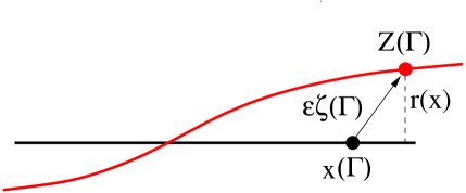
Figure 1: Schematic representation of the perturbation defined by (14).

Plugging (14) into (6), expanding the terms in this equation in a Taylor series in $\epsilon$ around $\epsilon=0$ and retaining terms proportional to $\epsilon$ yields

$${\partial\overline{\zeta}(t,\Gamma)\over\partial t}=\mathrm{i}({\mathcal{H}}\zeta)(t,\Gamma)+\mathrm{i}\overline{\zeta}(t,\Gamma),$$ (15)

where

$$({\mathcal{H}}\zeta)(t,\Gamma):=\frac{1}{2\pi}\mbox{f.p.}\int_{0}^{{{\widehat{\Gamma}}}}\frac{\zeta(t,\Gamma)-\zeta(t,\Gamma^{\prime})}{[x(\Gamma)-x(\Gamma^{\prime})]^{2}}\,\,\mathrm{d}\Gamma^{\prime}$$ (16)

is a hypersingular integral operator. The symbol “f.p.” indicates that the integral is understood in the sense of Hadamard’s finite part (Estrada & Kanwal, 2012). In the present problem the relation between the coordinates $\Gamma$ and $x$ in (16) is given in (9). It is illuminating to separate equation (15) into its real and imaginary parts using $\zeta=\zeta^{r}+\mathrm{i}\zeta^{i}$, leading to

$${\partial\zeta^{r}(t,\Gamma)\over\partial t} =-\left({\mathcal{H}}\zeta^{i}\right)(t,\Gamma)+\zeta^{i}(t,\Gamma),$$ (17a)

$${\partial\zeta^{i}(t,\Gamma)\over\partial t} =-\Big{(}{\mathcal{H}}\zeta^{r}\Big{)}(t,\Gamma)-\zeta^{r}(t,\Gamma).$$ (17b)

The integro-differential system (17) describes the evolution of infinitesimal perturbations to the equilibrium. Assuming that the real and imaginary parts of the perturbation depend on time as $\zeta^{r}(t,\Gamma)=\mathrm{e}^{\mathrm{i}\lambda t}\widehat{\zeta}^{r}(\Gamma)$ and $\zeta^{i}(t,\Gamma)=\mathrm{e}^{\mathrm{i}\lambda t}\widehat{\zeta}^{i}(\Gamma)$ turns (17) into the eigenvalue problem

$$\mathrm{i}\lambda\,\widehat{\zeta}^{r}(\Gamma) =-\left({\mathcal{H}}\widehat{\zeta}^{i}\right)(\Gamma)+\widehat{\zeta}^{i}(\Gamma),$$ (18a)

$$\mathrm{i}\lambda\,\widehat{\zeta}^{i}(\Gamma) =-\left({\mathcal{H}}\widehat{\zeta}^{r}\right)(\Gamma)-\widehat{\zeta}^{r}(\Gamma),$$ (18b)

where $\lambda\in{\mathbb{C}}$ is the eigenvalue and $\widehat{\zeta}^{r}$, $\widehat{\zeta}^{i}$ the corresponding eigenvectors.

Performing the same steps for the translating equilibrium described by (11)–(12) leads to the linearized system

$${\partial\zeta^{r}(t,\Gamma)\over\partial t} =-\left({\mathcal{G}}\zeta^{i}\right)(t,\Gamma),$$ (19a)

$${\partial\zeta^{i}(t,\Gamma)\over\partial t} =-\Big{(}{\mathcal{G}}\zeta^{r}\Big{)}(t,\Gamma),$$ (19b)

where the hypersingular integral operator ${\mathcal{G}}$ is defined as in (16), except that the relation between the coordinates $\Gamma$ and $x$ is now given in (13). The corresponding eigenvalue problem then takes the form

$$\mathrm{i}\lambda\,\widehat{\zeta}^{r}(\Gamma) =-\left({\mathcal{G}}\widehat{\zeta}^{i}\right)(\Gamma),$$ (20a)

$$\mathrm{i}\lambda\,\widehat{\zeta}^{i}(\Gamma) =-\left({\mathcal{G}}\widehat{\zeta}^{r}\right)(\Gamma).$$ (20b)

In principle, the linearized systems (17) and (19) have been obtained in a similar manner to the corresponding system in the case of the periodic vortex sheet (Saffman, 1992), except for a difference in the form of the kernel of the integral operator (16), more specifically how the coordinate $x$ depends on the integration variable $\Gamma^{\prime}$. and the presence of additional terms representing the background rotation in (17). In our analysis of eigenvalue problems (18) and (20) below it will be convenient to switch between parameterizations in terms of $\Gamma$ and $x$, which will be facilitated by relations (9) and (13).

3.1 Constraints on Admissible Perturbations

In order for perturbations $\zeta(t,\Gamma)$ to be physically admissible, they have to satisfy certain conditions. In the present problem we will require them to leave the total circulation ${\widehat{\Gamma}}$ of the sheet unchanged. Moreover, in the case of the rotating equilibrium we will also require the associated circulation densities to satisfy conditions (5), so that the velocity induced by the perturbed sheet remains everywhere bounded. In the case of the translating equilibrium, the analogous condition will require the perturbations to leave the type of singularity in the velocity field induced by the sheet near its endpoints unchanged. The main difficulty is that these conditions are naturally expressed in terms of the perturbed circulation density $\gamma$ which enters into (14) implicitly via the circulation parameter $\Gamma$. We thus need to translate these two conditions into constraints on the functions $\zeta(t,\Gamma)$.

In the rotating or translating frame of reference the perturbed sheet can be represented as the graph of a function $[x,r(x)]$, as in Figure 1, where the normal displacement $r(x)$ is related to the perturbation $\zeta(\Gamma)$ via

$$r(x)=\Im\,[Z(\Gamma(x))]=\epsilon\,\Im\,[\zeta(\Gamma(x))]$$ (21)

(for brevity, the dependence on time $t$ is omitted in this discussion). The circulation density $\gamma(x)$ is obtained from $\zeta(\Gamma)$ as follows

$$\left.\begin{aligned} \gamma(s)&=\frac{\mathrm{d}\Gamma}{\mathrm{d}s}=\left(\frac{\mathrm{d}s}{\mathrm{d}\Gamma}\right)^{-1}=\left({\partial Z\over\partial\Gamma}\,{\partial\overline{Z}\over\partial\Gamma}\right)^{-1/2}\\ {\partial{Z}\over\partial\Gamma}&={\partial x\over\partial\Gamma}+\epsilon{\partial\zeta\over\partial\Gamma}=\gamma_{0}^{-1}+\epsilon{\partial\zeta\over\partial\Gamma}\end{aligned}\right\}\quad\Longrightarrow$$

$$\begin{aligned} \gamma(s)&=\left[\left(\gamma_{0}^{-1}+\epsilon{\partial\zeta\over\partial\Gamma}\right)\left(\gamma_{0}^{-1}+\epsilon{\partial\overline{\zeta}\over\partial\Gamma}\right)\right]^{-1/2}\\ &=\gamma_{0}-\epsilon\,\gamma_{0}^{2}\,\Re\,\left[{\partial\zeta\over\partial\Gamma}\right]+O(\epsilon^{2})=\gamma_{0}\left[1-\epsilon{\partial\zeta^{r}\over\partial x}\right]+O(\epsilon^{2}),\end{aligned}$$ (22)

where we used the property $\gamma_{0}^{-1}\partial/\partial x=\partial/\partial\Gamma$.

The total circulation of the perturbed sheet is

$$\int_{0}^{{\widehat{\Gamma}}}\,d\Gamma =\int_{-1}^{1}\frac{\mathrm{d}\Gamma}{\mathrm{d}s}\frac{\mathrm{d}s}{\mathrm{d}x}\,\mathrm{d}x=\int_{-1}^{1}\left({\partial Z\over\partial\Gamma}\,{\partial\overline{Z}\over\partial\Gamma}\right)^{-1/2}\left({\partial Z\over\partial x}\,{\partial\overline{Z}\over\partial x}\right)^{1/2}\,\mathrm{d}x$$

$$=\int_{-1}^{1}\left[\left(\gamma_{0}^{-1}+\epsilon{\partial\zeta\over\partial\Gamma}\right)\left(\gamma_{0}^{-1}+\epsilon{\partial\overline{\zeta}\over\partial\Gamma}\right)\right]^{-1/2}\left[\left(1+\epsilon{\partial\zeta\over\partial x}\right)\left(1+\epsilon{\partial\overline{\zeta}\over\partial x}\right)\right]^{1/2}\,\mathrm{d}x$$

$$=\int_{-1}^{1}\left[\gamma_{0}-\epsilon\gamma_{0}^{2}\Re\,\left({\partial\zeta\over\partial\Gamma}\right)+O(\epsilon^{2})\right]\left[1+\epsilon\Re\,\left({\partial\zeta\over\partial x}\right)+O(\epsilon^{2})\right]\,\mathrm{d}x$$

$$=\int_{-1}^{1}\gamma_{0}(x)\,\mathrm{d}x+O(\epsilon^{2}),$$ (23)

where we have used (22). This relation implies that, to leading order in $\epsilon$, the total circulation is unaffected by perturbations of the form (14).

Hence the leading-order term in the expression for the perturbed circulation density is proportional to

$$\gamma_{0}(x){\partial\zeta^{r}\over\partial x}(\Gamma(x)).$$ (24)

In the case of the rotating equilibrium this term vanishes at the endpoints since $\gamma_{0}(\pm 1)=0$, provided $\zeta(\Gamma(x))\in C^{1}([-1,1])$. Under the same condition on $\zeta(\Gamma(x))$, the inverse square-root singularity of the circulation density in (12) is preserved in the case of the translating equilibrium. We thus conclude that the two constraints discussed above are satisfied automatically by perturbations $\zeta(\Gamma(x))$ that are continuously differentiable functions of $x$, such as polynomials. Hence there are no extra constraints to add to the eigenvalue problems (18) and (20).

3.2 Solution of Eigenvalue Problems (18) and (20)

In this section we present closed-form solutions to eigenvalue problems (18) and (20) corresponding to the rotating and translating equilibria. We remark that the form of these solutions was inspired by solutions to these problems obtained numerically using a spectral Chebyshev method, with complementary insights provided by Galerkin and collocation formulations (Boyd, 2001).

3.2.1 Eigenvalue Problem for the Rotating Equilibrium

We begin by expressing the hypersingular operator defined in (16) in terms of integrals defined in Cauchy’s principal-value sense as follows:

$$({\mathcal{H}}\zeta)(\Gamma(x)) =\frac{1}{2\pi}\mbox{f.p.}\int_{0}^{{{\widehat{\Gamma}}}}\frac{\zeta(\Gamma(x))-\zeta(\Gamma^{\prime})}{[x-x(\Gamma^{\prime})]^{2}}\,\mathrm{d}\Gamma^{\prime}=\frac{1}{2\pi}\mbox{f.p.}\int_{-1}^{1}\frac{\zeta(\Gamma(x))-\zeta(\Gamma(\xi))}{[x-\xi]^{2}}\gamma_{0}(\xi)\,\mathrm{d}\xi$$

$$=-\frac{1}{2\pi}\left[\zeta(\Gamma(x))\frac{\mathrm{d}}{\mathrm{d}x}\mbox{p.v.}\!\!\int_{-1}^{1}\frac{2\sqrt{1-\xi^{2}}}{x-\xi}\,\mathrm{d}\xi-\frac{\mathrm{d}}{\mathrm{d}x}\mbox{p.v.}\int_{-1}^{1}\frac{\zeta(\Gamma(\xi))2\sqrt{1-\xi^{2}}}{x-\xi}\,\mathrm{d}\xi\right],$$

$$=-\zeta(\Gamma(x))+\frac{1}{\pi}\frac{\mathrm{d}}{\mathrm{d}x}\mbox{p.v.}\!\!\int_{-1}^{1}\frac{\zeta(\Gamma(\xi))\sqrt{1-\xi^{2}}}{x-\xi}\,\mathrm{d}\xi,$$ (25)

where we have used (8) and the identity $\mbox{p.v.}\!\!\int_{-1}^{1}\sqrt{1-\xi^{2}}(x-\xi)^{-1}\,\mathrm{d}\xi=\pi x$. Next, applying this operator to the Chebyshev polynomial of the second type $U_{k}$ yields

$$({\mathcal{H}}U_{k})(x)=-U_{k}(x)+\frac{\mathrm{d}}{\mathrm{d}x}T_{k+1}(x)=kU_{k}(x),\qquad k=0,1,\dots,$$ (26)

where $T_{k}$ is the Chebyshev polynomial of the first kind. We have also used the identities $\mbox{p.v.}\!\!\int_{-1}^{1}\sqrt{1-\xi^{2}}U_{k-1}(\xi)(x-\xi)^{-1}\,\mathrm{d}\xi=\pi T_{k}(x)$ and $\mathrm{d}T_{k}/\mathrm{d}x=kU_{k-1}$ valid for $k\geq 1$ (DLMF, 2020). Relation (26) implies that $k=0,1,\dots$ and $U_{k}$ are, respectively, the eigenvalues and eigenvectors of the operator ${\mathcal{H}}$ in (16). We then rearrange problem (18) as

$$-\lambda^{2}\widehat{\zeta}^{r}=-({\mathcal{I}}-{\mathcal{H}})({\mathcal{I}}+{\mathcal{H}})\widehat{\zeta}^{r}=({\mathcal{H}}^{2}-{\mathcal{I}}^{2})\widehat{\zeta}^{r},$$ (27)

where ${\mathcal{I}}$ denotes the identity operator. Evidently, $\widehat{\zeta}^{r}(\Gamma(x))=U_{k}(x)$ is also an eigenfunction of problem (27) with the eigenvalue $\lambda_{k}=\pm\mathrm{i}\sqrt{k^{2}-1}$. Since $\widehat{\zeta}^{i}(\Gamma(x))$ satisfies an equation identical to (27), the solution of eigenvalue problem (18) is $\widehat{\zeta}^{r}_{k}(\Gamma(x))=U_{k}(x)$, $\widehat{\zeta}^{i}_{k}(\Gamma(x))=\theta_{k}U_{k}(x)$. Inserting this representation into (18) leads to $\theta_{k}=\sqrt{(k+1)/(k-1)}$ for $k=2,3,\dots$. The cases with $k=0,1$ need to be considered separately: the corresponding solutions can be easily deduced from (18). Thus the eigenvalues $\lambda_{k}$ and eigenvectors $\widehat{\zeta}_{k}=\widehat{\zeta}^{r}_{k}+\mathrm{i}\widehat{\zeta}^{i}_{k}$ of the problem (18) are

$$\lambda_{0} =\pm 1, \qquad\widehat{\zeta}_{0}(\Gamma) =1\pm\mathrm{i}^{2}=0,2,$$ (28a)

$$\lambda_{1} =0, \qquad\widehat{\zeta}_{1}(\Gamma) =\mathrm{i}x(\Gamma),$$ (28b)

$$\lambda_{k} =\pm\mathrm{i}\sqrt{k^{2}-1}, \widehat{\zeta}_{k}(\Gamma) =\left(1\pm\mathrm{i}\sqrt{\frac{k+1}{k-1}}\right)U_{k}(x(\Gamma)),\ k=2,3,\dots.$$ (28c)

The neutrally-stable mode (28a) represents harmonic oscillation of the centre of rotation around the origin. Mode (28b) associated with the zero eigenvalue represents the stretching or compression of the sheet, and can be therefore interpreted as connecting the rotating equilibrium defined by (7)–(8) with a nearby equilibrium. Finally, there exists a countably infinite family of linearly stable and unstable eigenmodes involving deformation of the sheet. In the limit of large $k$, the eigenvalues behave as $\lambda_{k}\sim\pm\mathrm{i}k$. The eigenfunctions (28c) corresponding to three different even and odd values of $k$ are shown in Figure 2 in terms of perturbed shapes and perturbed circulation densities of the vortex sheet.

        

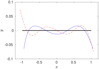
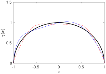
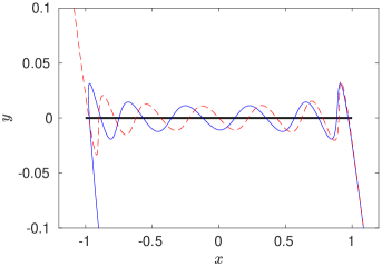
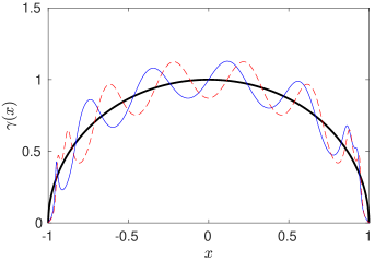
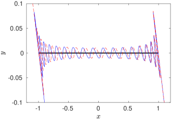
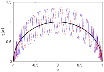
Figure 2: Unstable eigenvectors of the rotating equilibrium corresponding to (a,b) $k=4,5$, (c,d) $k=12,13$ and (e,f) $k=36,37$ in expressions (28c). The left column shows the perturbed sheet geometry $Z(\Gamma(x))$, and the right column the corresponding circulation density $\gamma(x)$, with $\epsilon=10^{-2}$. Solid blue and dashed red lines represent, respectively, the perturbations corresponding to even and odd values of $k$, while thick black lines represent the equilibrium configuration.

3.2.2 Eigenvalue Problem for the Translating Equilibrium

Analogously to (25), the action of the hypersingular operator ${\mathcal{G}}$ on the perturbation $\zeta$ can be expressed using (12) as

$$({\mathcal{G}}\zeta)(\Gamma(x)) =\frac{1}{2\pi}\mbox{f.p.}\int_{-1}^{1}\frac{\zeta(\Gamma(x))-\zeta(\Gamma(\xi))}{[x-\xi]^{2}}\gamma_{0}(\xi)\,\mathrm{d}\xi=\frac{1}{2\pi}\mbox{f.p.}\int_{-1}^{1}\frac{\zeta(\Gamma(x))-\zeta(\Gamma(\xi)}{[x-\xi]^{2}}\frac{2\xi}{\sqrt{1-\xi^{2}}}\,\mathrm{d}\xi$$

$$=-\frac{1}{\pi}\left[\zeta(\Gamma(x))\frac{\mathrm{d}}{\mathrm{d}x}\mbox{p.v.}\int_{-1}^{1}\frac{\xi}{\sqrt{1-\xi^{2}}(x-\xi)}\,\mathrm{d}\xi-\frac{\mathrm{d}}{\mathrm{d}x}\mbox{p.v.}\int_{-1}^{1}\frac{\zeta(\Gamma(\xi))\xi}{\sqrt{1-\xi^{2}}(x-\xi)}\,\mathrm{d}\xi\right],$$

$$=\frac{1}{\pi}\frac{\mathrm{d}}{\mathrm{d}x}\mbox{p.v.}\int_{-1}^{1}\frac{\zeta(\Gamma(\xi))\xi}{\sqrt{1-\xi^{2}}(x-\xi)}\,\mathrm{d}\xi,$$ (29)

where we have used the identity $\mbox{p.v.}\!\!\int_{-1}^{1}\xi(1-\xi^{2})^{-1/2}(x-\xi)^{-1}\,\mathrm{d}\xi=-\pi$. Representing the perturbation as a function of $x$ in terms of a Chebyshev series expansion with complex coefficients

$$\zeta(\Gamma(x))=\sum_{k=0}^{\infty}(\alpha_{k}+i\beta_{k})T_{k}(x),\qquad\alpha_{k},\beta_{k}\in{\mathbb{R}},\qquad k=0,1,\dots,$$ (30)

we have $({\mathcal{G}}\zeta)(x)=\sum_{k=0}^{\infty}(\alpha_{k}+\mathrm{i}\beta_{k})({\mathcal{G}}T_{k})(x),$ where

$$({\mathcal{G}}T_{k})(x)=\frac{1}{\pi}\frac{\mathrm{d}}{\mathrm{d}x}\mbox{p.v.}\int_{-1}^{1}\frac{\xi T_{k}(\xi)}{\sqrt{1-\xi^{2}}(x-\xi)}\,\,\mathrm{d}\xi,\qquad k\geq 0.$$ (31)

Using the identity $\mbox{p.v.}\!\!\int_{-1}^{1}T_{k}(\xi)(1-\xi^{2})^{-1/2}(x-\xi)^{-1}\,\mathrm{d}\xi=-\pi U_{k-1}(x)$, $k\geq 1$, and the recurrence relations characterizing the Chebyshev polynomials of the first and second kind (DLMF, 2020), we find

$$({\mathcal{G}}T_{0})(x) =0,$$ (32a)

$$({\mathcal{G}}T_{k})(x) =\frac{1}{1-x^{2}}\left[kxT_{k}(x)-U_{k-1}(x)\right],\qquad k=1,2,\dots.$$ (32b)

We then define

$${\mathbf{w}}(t) :=\left[\alpha_{0}(t),\alpha_{1}(t),\dots,\beta_{0}(t),\beta_{1}(t),\dots\right]^{T},$$ (33a)

$$[{\bf G}]_{jk} :=\int_{-1}^{1}\frac{T_{j}(\xi)({\mathcal{G}}T_{k})(\xi)}{\sqrt{1-\xi^{2}}}\,\mathrm{d}\xi,\quad j,k=0,1,\dots,$$ (33b)

where the last expression represents the $j$th Chebyshev coefficient of $({\mathcal{G}}T_{k})(x)$. Then the system (19) can be rewritten as an infinite-dimensional vector equation

$$\frac{d}{dt}{\mathbf{w}}=\begin{bmatrix}\phantom{-}{\mathbf{0}}&-{\bf G}\\ -{\bf G}&\phantom{-}{\mathbf{0}}\end{bmatrix}{\mathbf{w}}=:{\bf A}{\mathbf{w}},$$ (34)

where ${\mathbf{0}}$ represents the null matrix. We remark that when the operator ${\mathcal{G}}$ acts on a polynomial, the result is a polynomial of degree reduced by one. Thus, matrix ${\bf G}$ representing this operator in the Chebyshev basis is upper triangular with zeros on its main diagonal. Therefore, we conclude that zero is the only eigenvalue of the operator ${\mathcal{G}}$ and hence also of the eigenvalue problem (20). The relation (32a) indicates that $\widehat{\zeta}^{r}(\Gamma)=\widehat{\zeta}^{i}(\Gamma)=1$ is the only eigenvector, which implies that the eigenvalue $\lambda=0$ has infinite algebraic multiplicity and geometric multiplicity equal to 1. The matrix ${\bf A}$ is nilpotent of degree infinity.

In the presence of such an extreme form of degeneracy, solutions of system (34) corresponding to some initial condition ${\mathbf{w}}_{0}\in l^{2}$ can be written as (Perko, 2008)

$${\mathbf{w}}(t)=\mathrm{e}^{t{\bf A}}{\mathbf{w}}_{0}={\bf P}\operatorname{diag}\{\mathrm{e}^{\lambda_{j}t}\}{\bf P}^{-1}\left[{\bf I}+t{\bf A}+\frac{t^{2}}{2}{\bf A}^{2}+\dots\right]{\mathbf{w}}_{0}=\left[{\bf I}+t{\bf A}+\frac{t^{2}}{2}{\bf A}^{2}+\dots\right]{\mathbf{w}}_{0},$$ (35)

where ${\bf I}$ is the identity matrix and ${\bf P}:=[{\mathbf{v}}_{0},{\mathbf{v}}_{1},\dots]$ is a matrix with columns given by the generalized eigenvectors ${\mathbf{v}}_{k}$, $k=0,1,\dots$ obtained from the Jordan chain (Perko, 2008)

$${\bf A}{\mathbf{v}}_{1} ={\mathbf{v}}_{0}=\left[1,0,\dots,1,0,\dots\right]^{T},$$ (36a)

$${\bf A}{\mathbf{v}}_{k+1} ={\mathbf{v}}_{k},\qquad k=1,2,\dots.$$ (36b)

Because of property (32b), the Jordan chain of generalized eigenvectors consists of polynomials of degree increasing with $k$, and ${\mathbf{v}}_{k}$ represents the Chebyshev coefficients of a polynomial of degree $k$. Since the generalized eigenvectors are linearly independent, the matrix ${\bf P}$ is invertible. As all the eigenvalues are equal to zero, the product of the first three factors on the first line in expression (35) reduces to the identity matrix. Expanding the initial condition in terms of the generalized eigenvectors from the Jordan chain (36) as ${\mathbf{w}}_{0}=\eta_{0}{\mathbf{v}}_{0}+\eta_{1}{\mathbf{v}}_{1}+\dots$ for some $\eta_{0},\eta_{1},\dots\in{\mathbb{R}}$ and using the property that ${\bf A}^{j}{\mathbf{v}}_{k}={\mathbf{0}}$ for $0\leq k<j$, we can rewrite the solution (35) as

$${\mathbf{w}}(t)={\mathbf{w}}_{0}+t(\eta_{1}{\mathbf{v}}_{1}+\eta_{2}{\mathbf{v}}_{2}+\dots)+\cdots+\frac{t^{n}}{n!}(\eta_{n}{\mathbf{v}}_{n}+\eta_{n+1}{\mathbf{v}}_{n+1}+\dots)+\cdots,\qquad 2<n<\infty.$$ (37)

This form of the solution allows us to conclude that, for each integer $n>0$, there exists a perturbation ${\mathbf{w}}_{0}$ given by a polynomial of degree equal to or greater than $n$ which grows in time at a rate proportional to at least $t^{n}$.

In order to understand the structure of the fastest-growing perturbations represented by (37), it is instructive to examine the generalized eigenvectors defined in (36) as functions of $x\in[-1,1]$, i.e. $v_{k}(x)=\sum_{j=0}^{k}[{\mathbf{v}}_{k}]_{j}T_{j}(x)$, $k=0,1,\dots$. The first six generalized eigenvectors then take the form

$$v_{0}(x) =T_{0}(x)=1, \qquad v_{1}(x) =T_{1}(x)=x,$$ (38a)

$$v_{2}(x) =\frac{1}{4}T_{2}(x)=\frac{1}{2}x^{2}-\frac{1}{4}, \qquad v_{3}(x) =\frac{1}{24}T_{3}(x)-\frac{5}{24}T_{1}(x)=\frac{1}{6}x^{3}-\frac{1}{3}x,$$ (38b)

$$v_{4}(x) =\frac{1}{192}T_{4}(x)-\frac{7}{96}T_{2}(x) \qquad v_{5}(x) =\frac{1}{1920}T_{5}(x)-\frac{9}{640}T_{3}(x)+\frac{61}{960}T_{1}(x)$$

$$=\frac{1}{24}x^{4}-\frac{3}{16}x^{2}+\frac{5}{64}, =\frac{1}{120}x^{5}-\frac{1}{15}x^{3}+\frac{13}{120}x$$ (38c)

and some of them are plotted in Figure 3. The remaining generalized eigenvectors follow the same pattern. We observe that the generalized eigenvectors of even order consist of even-degree polynomials only and vice versa. In all cases the magnitude of the coefficients decreases with the degree of the term, so that the form of the generalized eigenvectors is dominated by their lower-degree terms. As a result, while the generalized eigenvectors (38) are linearly independent (Perko, 2008), they form a strongly non-normal set, as shown in Figure 3. This implies that when the initial perturbation $\zeta(0,\Gamma(x))$ in the form of a generic degree-$n$ polynomial of $x$ is expanded in terms of the generalized eigenvectors (38), the expansion coefficients $\eta_{k}$, $k=0,1,\dots,n$ generically increase in magnitudes with $k$. This means that the fastest-growing components of such an initial perturbation will be given by the generalized eigenvector $v_{n}$, and will grow at a rate proportional to $t^{n}$. We also remark that the even-degree generalized eigenvectors shown in Figure 3 have some resemblance to the form of the most amplified perturbations observed during the time evolution of a perturbed Prandtl-Munk vortex. More precisely, while the linear stability analysis cannot predict the roll-up of the sheet near its endpoints which is driven by nonlinear effects, it does appear to capture the change of the global shape of the sheet as in Figure 2 in Krasny (1987) and Figure 4 in DeVoria & Mohseni (2018). However, given the form (37) of the solution of the linearized problem, it is impossible to make this statement more quantitative, e.g. by comparing the growth rates.

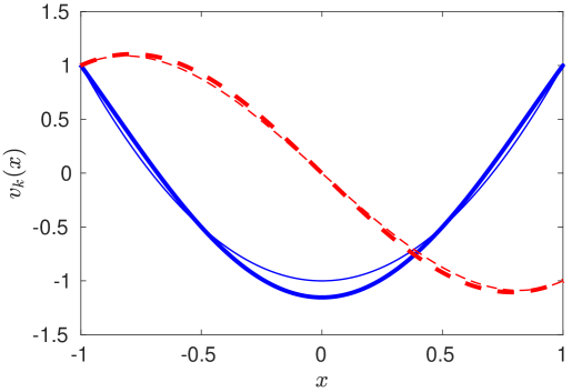
Figure 3: Generalized eigenvectors $v_{2}$, $v_{4}$ (blue solid lines) and $v_{3}$, $v_{5}$ (red dashed lines) as functions of $x$. Thicker lines represent generalized eigenvectors of a higher degree. The graphs of the remaining generalized eigenvectors $v_{6}$ ,$v_{7}$, $\dots$ are essentially indistinguishable from the thicker curves.

4 Time-dependent straight vortex sheets

The relative equilibrium involving Kirchhoff’s rotating ellipse has been generalized by including the effect of linear velocity fields. Moore & Saffman (1971) found steady states involving ellipses in a uniform straining field, while time-dependent solutions in the presence of a simple shear were investigated by Kida (1981). In this section we describe analogous generalizations of the rotating equilibria of the vortex sheet described in § 2.1, whereas in § 5.2 it is demonstrated that some of these solutions in fact coincide with the infinite-aspect-ratio limits of the Moore-Saffman and Kida vortex-patch solutions (Moore & Saffman, 1971; Kida, 1981). An alternative derivation of these solutions will be presented in Appendix A.

4.1 Governing equations

We now derive from first principles the equation of motion for a single vortex sheet in the presence of a linear external flow given by $F(z)=Az+B{\overline{z}}$ with $A,B\in\mathbb{C}$. Our focus is on solutions in which the vortex sheet retains the form of a straight segment, but with varying length and inclination angle to the coordinate axes. Since the external flow should be divergence-free, we have $\Re\,[(\partial_{x}-i\partial_{y})F(z)]=\Re\,[B]=0$. Hence, without loss of generality, we can set the parameters of the external flow as $A=r\mathrm{e}^{-\mathrm{i}\theta_{0}}$ and $B=\mathrm{i}\Omega$, where $r>0$, $\Omega\in\mathbb{R}$ and $\theta_{0}\in(0,2\pi)$. This form of the external flow is a generalization of the earlier studies mentioned: Kida’s case (Kida, 1981) corresponds to $\theta_{0}=0$, while $\Omega=0$ leads to Moore’s and Saffman’s case (Moore & Saffman, 1971). The evolution of the vortex sheet represented by the curve ${\mathcal{L}}(t)\in{\mathbb{C}}$ is then governed by the augmented Birkhoff-Rott equation (6), which becomes

$${\partial\overline{z}\over\partial t}=\frac{1}{2\pi\mathrm{i}}\mbox{p.v.}\int_{\mathcal{L}}\frac{\gamma(w)}{z-w}|\mathrm{d}w|+r\mathrm{e}^{-\mathrm{i}\theta_{0}}z+\mathrm{i}\Omega\overline{z},\qquad z\in{\mathcal{L}}.$$ (39)

We now assume that the vortex sheet has the form of a line segment and therefore can be parameterized as

$${\mathcal{L}}(t)\;\colon\;z(t,s)=a(t)s\mathrm{e}^{\mathrm{i}\theta(t)},\qquad\mbox{where $-1\leq s\leq 1$}.$$ (40)

The positive-valued function $a(t)$ represents the half-length of the vortex sheet, while the real-valued function $\theta(t)$ gives the angle between $x$-axis and the sheet. Although the support ${\mathcal{L}}(t)$ of the circulation density changes in time, the total circulation ${\widehat{\Gamma}}$ carried by the vortex sheet must be conserved in time. Hence, we take the circulation density to have a form analogous to (8), with

$$\gamma(z)=\frac{2}{a(t)}\sqrt{1-\frac{z^{2}}{a^{2}(t)\mathrm{e}^{2\mathrm{i}\theta(t)}}},\qquad z\in{\mathcal{L}}(t).$$ (41)

Then the total circulation is independent of $a(t)$ and $\theta(t)$, and

$${\widehat{\Gamma}}=\int_{{\mathcal{L}}(t)}\gamma(z)|\mathrm{d}z|=\int_{-1}^{1}\frac{2}{a(t)}\sqrt{1-\frac{a^{2}(t)s^{2}\mathrm{e}^{2\mathrm{i}\theta(t)}}{a^{2}(t)\mathrm{e}^{2\mathrm{i}\theta(t)}}}a(t)\,\mathrm{d}s=\int_{-1}^{1}2\sqrt{1-s^{2}}\,\mathrm{d}s=\pi.$$ (42)

Equations for $a(t)$ and $\theta(t)$ are obtained by substituting (40) and (41) into (39). The singular integral in (39) then becomes

$$\mbox{p.v.}\int_{\gamma}\frac{\gamma(w)}{z-w}|dw| =\mbox{p.v.}\int_{-1}^{1}\frac{2\sqrt{1-(s^{\prime})^{2}}}{a(t)s\mathrm{e}^{\mathrm{i}\theta(t)}-a(t)s^{\prime}\mathrm{e}^{\mathrm{i}\theta(t)}}\,\mathrm{d}s^{\prime}$$ (43)

$$=\frac{\mathrm{e}^{-\mathrm{i}\theta(t)}}{a(t)}\mbox{p.v.}\int_{-1}^{1}\frac{2\sqrt{1-(s^{\prime})^{2}}}{s-s^{\prime}}\,\mathrm{d}s^{\prime}=\frac{2\pi s}{a(t)}\mathrm{e}^{-\mathrm{i}\theta(t)},$$ (44)

where we have used the fact that the Hilbert transform of $\sqrt{1-s^{2}}$ is $\pi s$. After performing some elementary algebraic operations we obtain

$$\begin{bmatrix}\dot{a}(t)\\ \dot{\theta}(t)\end{bmatrix}=\begin{bmatrix}a(t)r\cos(2\theta(t)-\theta_{0})\\ \frac{1}{a^{2}(t)}-r\sin(2\theta(t)-\theta_{0})-\Omega\end{bmatrix}.$$ (45)

As shown in Appendix A, this system can also be derived using an approach proposed by O’Neil (2018a, b) to construct equilibrium solutions involving vortex sheets.

The well-posedness of system (45) is easily established. Rewriting the first equation in (45) as $a^{-1}\dot{a}=r\cos(2\theta(t)-\theta_{0})$, we immediately see that

$$a(t)=a(0)\exp\left[r\int_{0}^{t}\cos(2\theta(s)-\theta_{0})\,\mathrm{d}s\right].$$ (46)

Since $-1\leqq\cos(2\theta(t)-\theta_{0})\leqq 1$ for all $t\in\mathbb{R}$, we have

$$0<a(0)\exp\left(-rt\right)\leqq a(t)\leqq a(0)\exp\left(rt\right)<\infty.$$

This means the solutions of (45) cannot blow up in finite time, but unbounded growth is possible in infinite time, in the sense that $a(t)\rightarrow\infty$ as $t\to\pm\infty$ as we shall see below.

4.2 Analysis of the fixed points of the system (45)

Fixed points of the system (45) are obtained directly by solving the equations $\dot{a}=\dot{\theta}=0$. From $\dot{a}=ar\cos(2\theta-\theta_{0})=0$ it immediately follows that $\theta=\theta_{n}:=\frac{\theta_{0}}{2}+\frac{\pi}{4}+\frac{n\pi}{2}$ for $n\in\mathbb{Z}$. Since $\sin(2\theta_{n}-\theta_{0})=(-1)^{n}$, $\dot{\theta}=0$ is equivalent to $a^{-2}=r+\Omega$ when $\theta=\theta_{2m}$ and to $a^{-2}=-r+\Omega$ when $\theta=\theta_{2m+1}$, $m\in{\mathbb{Z}}$. Hence, when $\Omega>r$, we have the following two families of steady states

$$(a_{2m},\theta_{2m}) =\left(\frac{1}{\sqrt{r+\Omega}},\frac{\theta_{0}}{2}+\frac{\pi}{4}+m\pi\right),$$ (47a)

$$(a_{2m+1},\theta_{2m+1}) =\left(\frac{1}{\sqrt{-r+\Omega}},\frac{\theta_{0}}{2}+\frac{\pi}{4}+\left(m+\frac{1}{2}\right)\pi\right),\qquad m\in{\mathbb{Z}}.$$ (47b)

On the other hand, when $r>\Omega>-r$, there is only one family of steady states given by (47a) and there are no steady states when $\Omega<-r$. Since in the fixed frame of reference considered here the relative equilibrium discussed in § 2.1 has the form of a periodic solution, in the limit $r,\Omega\rightarrow 0^{+}$ the fixed points (47) disappear to infinity.

We now analyze trajectories near the fixed points (47). We emphasize that this is not a stability analysis of the equations motion as was carried out in § 3.2.1; instead, here we focus on perturbations which only affect $a(t)$ and $\theta(t)$ in (40), i.e. those that leave the vortex sheet in the form of a straight segment. The Jacobian of system (45) is given by

$$\begin{bmatrix}r\cos(2\theta-\theta_{0})&-2ar\sin(2\theta-\theta_{0})\\ -2a^{-3}&-2r\cos(2\theta-\theta_{0})\end{bmatrix}.$$ (48)

Computing the eigenvalues of Jacobian (48) evaluated at the critical points yields

• $\lambda=\pm 2\sqrt{r(r+\Omega)}$ for the critical points (47a) when $r+\Omega>0$, indicating that these critical points are saddles,

• $\lambda=\pm 2\sqrt{r(-r+\Omega)}\,i$ for the critical points (47b) when $\Omega>r$, indicating that these critical points are centres.

The structure of the phase space $(a,\theta)$ of system (45) for different combinations of the parameters $r$ and $\Omega$ is explored in the next section.

4.3 Phase plots

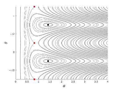
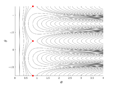
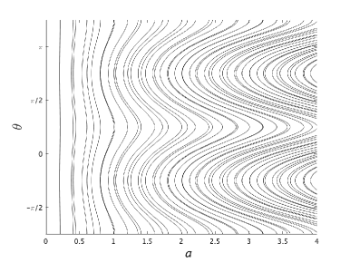
Figure 4: Solution trajectories of system (45) in the phase space $(a,\theta)\in{\mathbb{R}}_{+}\times{\mathbb{R}}$ for different choices of parameters: (a) $(r,\Omega)=(0.5,1.0)$, (b) $(r,\Omega)=(1.0,0.5)$ and (c) $(r,\Omega)=(0.5,-1.0)$. The black and red solid symbols represent centres and saddles as given in (47a) and (47b).

The phase space $(a,\theta)\in{\mathbb{R}}_{+}\times{\mathbb{R}}$ of the system (45) is characterized by solving it numerically with different initial conditions $(a(0),\theta(0))$. The results are shown in Figure 4 for the following three cases: (a) $\Omega>r$, (b) $r>\Omega>-r$ and (c) $-r>\Omega$. Without loss of generality, we choose $\theta_{0}=0$, since this parameter controls only the inclination angle of the equilibrium configurations and not their stability.

When $r=0.5$ and $\Omega=1.0$, the steady states $(a_{2m},\theta_{2m})$ are centres and those at $(a_{2m+1},\theta_{2m+1})$ are saddles with heteroclinic connections; see Figure 4(a). In the neighborhood of the centres the orbits are periodic representing oscillation of the sheet without rotation. Outside the heteroclinic connections, the solutions involve rotation of the sheet. The direction of rotation for initial data located to the left of the heteroclinic orbits is opposite to that for initial data located to the right of the heteroclinic orbits.

For $r=1.0$ and $\Omega=0.5$, the steady states at $(a_{2m+1},\theta_{2m+1})$ are saddle points linked by heteroclinic connections, as seen in Figure 4(b). Orbits to the left of the heteroclinic connections represent periodic solutions for which the sheet rotates in the counter-clockwise direction while its length oscillates. This is because in the second equation in system (45) we obtain $\dot{\theta}\sim\frac{1}{2a^{2}}>0$ for sufficiently small $a$. On the other hand, orbits to the right of the heteroclinic connection represent unbounded solutions in which the length of the vortex sheet goes to infinity as $t\rightarrow\infty$ while the inclination angle $\theta$ asymptotically approaches a constant angle $\theta_{\infty}:=-\frac{\pi}{12}+\frac{m\pi}{2}$, $m\in{\mathbb{Z}}$, which satisfies the relation $\Omega+r\sin 2\theta_{\infty}=0$.

For $r=0.5$ and $\Omega=-1.0$, we observe only periodic orbits in which the vortex sheet is rotating in the counter-clockwise direction; see Figure 4(c). Longer sheets exhibit a more significant variation of their length during one period of rotation.

We reiterate that in the analysis presented in this section we restricted our attention to those solutions only where the sheet retains the form of a straight segment with variable length and inclination angle. Determining the effect of external fields on motions of the vortex sheet involving arbitrary deformations remains an open problem.

5 Relation between Rotating Sheets and Ellipses

5.1 Stability Analysis Based on Limit of Kirchhoff’s Rotating Ellipse

We first list stability results for Kirchhoff’s ellipse following Love (1893) who first found instability for $a/b>3$, where $a$ and $b$ are, respectively, the semi-major and semi-minor axis of the ellipse, and then investigate the limit of large aspect ratio $a/b$. Following the notation of Mitchell & Rossi (2008), the dimensional frequency, $\lambda_{*}$, of a mode-$m$ disturbance satisfies

$$\lambda_{*}^{2}=\frac{\omega^{2}}{4}\left[\left(\frac{2mab}{(a+b)^{2}}-1\right)^{2}-\left(\frac{a-b}{a+b}\right)^{2m}\right],$$ (49)

where $\omega$ is the value of the constant vorticity inside the ellipse and $m>0$. Now consider the limit of (49) as $b/a$ tends to $0$, with the circulation, ${\widehat{\Gamma}}=\pi\omega ab$, kept constant. This leads to

$$\lambda_{*}^{2}=\frac{\omega^{2}b^{2}}{a^{2}}(2m-m^{2})+o(1).$$ (50)

This is negative for $m>2$, so that modes with $m>2$ are unstable. The growth rate increases with $m$, a characteristic sign of ill-posedness. We nondimensionalize $\lambda_{*}$ using the dimensional angular velocity $\Omega_{*}=\omega ab/(a+b)^{2}$ of the ellipse. This angular velocity tends to $\omega b/a$ as $b/a\to 0$, so we obtain the nondimensional frequency

$$\lambda=\frac{\lambda_{*}}{\Omega_{*}}=\pm\mathrm{i}\sqrt{m^{2}-2m}=\pm\mathrm{i}[(m-1)^{2}-1]^{1/2}.$$ (51)

To relate this result to the vortex sheet frequencies given by (28a)–(28c), we note that the Cartesian mode number $k$ is related to the azimuthal mode number $m$ by $m=k+1$, as in (16a–b) of Mitchell & Rossi (2008). We see that the unstable growth rates with $m>2$ correspond to (28c). The neutral mode $m=2$ corresponds to (28b). The stable oscillations with $m=1$ correspond to (28a). This limiting process is illustrated in Figure 5 where we show Kirchhoff’s elliptic vortex with aspect ratio 100 together with its deformation by the highest-wavenumber unstable mode predicted by Love’s analysis (Love, 1893; Mitchell & Rossi, 2008), which for the given aspect ratio corresponds to $m=64$. In Figure 5 we note the emergence of a deformation pattern in the form of a slanted wave which is also evident in Figures 2a,c,e.

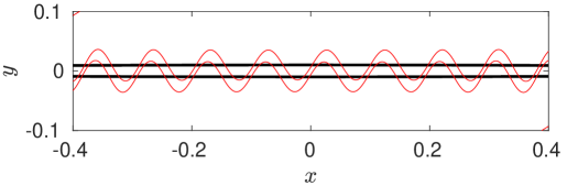
Figure 5: (Thick solid line) a section of Kirchhoff’s elliptic vortex with aspect ratio 100 together with (thin red line) its deformation by the unstable mode with wavenumber $m=64$.

5.2 Limit of Kirchhoff’s ellipse in the presence of external fields

The generalizations of the rotating equilibrium of a vortex sheet described in § 2.1 can be obtained by considering suitable limits of the evolution of Kirchhoff’s ellipse in the presence of external fields. Our discussion of the generalizations of Kirchhoff’s elliptical vortex follows § 9.3 in Saffman (1992). Given a prescribed strain $U-\mathrm{i}V=(\mathrm{i}e(t)+g(t))z$, where $e(t)$ and $g(t)$ are real-valued functions of time, there exist time-dependent patch solutions with constant vorticity $\omega$ in the form of rotating ellipses whose semi-major and semi-minor axes $a(t)$ and $b(t)$ vary with time and the semi-major axis makes an angle $\theta(t)$ with the $x$-axis, as described by equations (19)–(20) in § 9.3 of Saffman (1992). Taking the limit $b\to 0$ with constant circulation ${\widehat{\Gamma}}=\pi\omega a(t)b(t)$ so that $\omega\to\infty$, we obtain the equations governing the evolution of the vortex sheet in the prescribed strain in terms of its half-length $a(t)$ and inclination angle $\theta(t)$ in the form

$$\dot{a}=-ea\sin{2\theta}+ga\cos{2\theta},\qquad\dot{\theta}=\frac{{\widehat{\Gamma}}}{\pi a^{2}}-e\cos{2\theta}-g\sin{2\theta}.$$ (52)

The circulation density of the sheet is then $2{\widehat{\Gamma}}\sqrt{1-s^{2}/a(t)^{2}}/(\pi a(t))$, where $s\in[0,a(t)]$ is distance from the origin. It is clear that in the absence of the external strain ($e=g=0$) we recover the rotating equilibrium discussed in § 2.1. Moreover, the equations are equivalent to (45) when we consider the single vortex sheet (40) with circulation ${\widehat{\Gamma}}=\pi$ in steady external strain, i.e. $e=-r\sin\theta_{0}$ and $g=r\cos\theta_{0}$, with $\Omega=0$.

The Moore–Saffman solutions are steady states involving ellipses in a uniform straining field (Moore & Saffman, 1971). The corresponding vortex sheet equilibrium can be obtained without loss of generality by taking $g=0$ in (52), which yields $\dot{a}=0$, $\theta=0$ along with $e={\widehat{\Gamma}}/(\pi a^{2})$. Saffman (1992) points out that if patches do not satisfy the appropriate condition, “the vortex is pulled out into a long thin ellipse along the principal axis of extension.” Since the vortex sheet already has zero thickness, such circumstances will result in unbounded growth of the sheet length $a(t)$ accompanied by the vanishing of its circulation density. The effect of solid-body rotation represented by an extra term of the form $-\mathrm{i}\Omega_{0}\overline{z}$ was considered by Kida (1981). In terms of the evolution of the vortex sheet the only difference is an extra term $\Omega$ in the equation for $\dot{\theta}$ in (52), and this recovers (45) for the case of steady strain with rotation $\Omega$.

6 Discussion and Conclusions

In this study we have established a number of new results concerning the stability of the rotating and translating equilibria of open finite vortex sheets. Some of these findings complement analogous results already known for unbounded, periodic and circular vortex sheets. The main difference between these two types of equilibria, and at the same time the source of several technical difficulties here, is the presence of the endpoints.

The stability analysis of rotating equilibria shows similar behavior to straight periodic sheets (Saffman, 1992) and circular sheets (Michalke & Timme, 1967). More specifically, there is a countably infinite family of unstable modes with growth rates increasing with the wavenumber $k$, as shown in (28c). Away from the endpoints and in the limit of large wavenumbers the corresponding unstable eigenmodes resemble the unstable eigenmodes of a straight periodic sheet which have the form $(1-\mathrm{i})\sin(k\xi)$, $\xi\in[0,2\pi]$. More precisely, near the centre of the sheet the unstable eigenmodes have the form of slanted sine and cosine waves. The reason for this analogy can be understood by examining the structure of the eigenvalue problem (18) and the hypersingular integral operator (25). We see that when the eigenvalues $\lambda$ have large magnitude, the terms due to the background rotation in (18) are dominated by the other terms. Moreover, when the integral operator ${\mathcal{H}}$ acts on high-wavenumber perturbations $\zeta(\Gamma(x))$, the circulation density $\gamma_{0}(x)$ in (8) can be locally approximated by a constant for $x$ away from the endpoints. Thus, in this limit, the structure of the eigenvalue problem (18) becomes similar to the structure of the eigenvalue problem characterizing the stability of straight periodic vortex sheets (Saffman, 1992). Therefore, we can conclude that rotating finite sheets are subject to the same Kelvin–Helmholtz instability as straight sheets, which becomes more severe at higher wavenumbers and rendering this problem similarly ill-posed.

On the other hand, the solution of the stability problem for the translating vortex sheet in § 3.2.2 is more nuanced since, as a result of the degeneracy of the eigenvalue problem (20) with the hypersingular integral operator (29), this equilibrium sustains unstable modes growing at an algebraic rather than exponential rate. However, this algebraic growth rate can be arbitrarily large provided the perturbations vary sufficiently rapidly in space. Thus, this problem is ill-posed in a similar way to vortex sheets exhibiting the classical Kelvin-Helmholtz instability. As suggested by the form of the generalized eigenvectors shown in Figure 3, this analysis captures the general form of the instability actually observed in numerical computations (Krasny, 1987; DeVoria & Mohseni, 2018), although direct comparisons are made difficult by the fact that the computations relied on various regularized forms of the Birkhoff-Rott equation (3), while no such regularization was used in our stability analysis. The Prandtl-Munk vortex is thus the only known equilibrium involving a vortex sheet which does not have exponentially unstable modes. This property can be attributed to the fact that the corresponding circulation density (12) is not sign-definite, so that the self-induced straining field exerts a stabilizing effect.

The results reported in § 4 show that the rotating equilibrium discussed in § 2.1 is “robust” in the sense that configurations involving straight sheets but with time-dependent length and inclination angle also arise as solutions in the presence of external fields. However, we remark that the results presented in § 4.2 do not represent a complete stability analysis since they do not account for perturbations affecting the shape of the sheet. Generalizing this analysis to account for such shape-deforming perturbations is thus an open problem. For the periodic solutions of Figure 4a, this could be done by combining the methods from § 3 with Floquet theory. Another interesting open question is whether the translating equilibrium admits generalizations analogous to those discussed in § 4.

The analysis presented in § 5 demonstrates that the relation between the rotating vortex sheet and Kirchhoff’s ellipse stipulated by Batchelor (1988) does not merely concern the form of the equilibrium configurations, but also applies to their stability properties. That this should be the case seems nontrivial because in the infinite-aspect-ratio limit the form of the Euler equation used to describe vortex patches and its linearization lose validity. The practical value of the stability results obtained in § 3 is their simple and explicit form making comparisons with stability analyses of other configurations such a straight infinite vortex sheet straightforward. In contrast, the expressions describing unstable modes of Kirchhoff ellipse obtained by Love (1893) are rather complicated. The relation between the evolution of unbounded sheets of finite and zero thickness was considered by Baker & Shelley (1990); Benedetto & Pulvirenti (1992). An interesting open question is whether there exists a family of vortex-patch equilibria that will converge to the Prandtl-Munk vortex in a certain limit. Another open problem is to understand whether the equilibria considered here are unique in the class of configurations involving a single open finite vortex sheet.

Appendix A Derivation of solutions from § 4 following O’Neil’s formulation

In this appendix we show that the solutions obtained in § 4 as generalizations of the rotating equilibrium from § 2.1 can be obtained in an entirely different manner using the method of O’Neil (2018a, b).

We begin with vortex sheet equilibria in the presence of uniform strain without rotation. The velocity field due to the sheet ${\mathcal{L}}$ and the strain field is

$$f(z)=\frac{1}{2\pi\mathrm{i}}\int_{\mathcal{L}}\frac{\gamma(w)\overline{\tau}(w)}{z-w}\,\mathrm{d}w+r\mathrm{e}^{-\mathrm{i}\theta_{0}}z,\qquad z\notin{\mathcal{L}}.$$ (53)

The argument of O’Neil (2018a, b) shows that the extension of $f^{2}(z)$ in the finite plane including the sheet ${\mathcal{L}}$ is entire. At infinity, we find

$$f^{2}(z) =\left[r\mathrm{e}^{-\mathrm{i}\theta_{0}}z+\frac{1}{2\pi\mathrm{i}z}\int_{\mathcal{L}}\gamma(w)\,|\mathrm{d}w|+O(|z|^{-2})\right]^{2}=r^{2}\mathrm{e}^{-2\mathrm{i}\theta_{0}}z^{2}+\frac{{\widehat{\Gamma}}r\mbox{e}^{-\mathrm{i}\theta_{0}}}{\pi\mathrm{i}}+O(|z|^{-1}),$$

$$=r^{2}\mathrm{e}^{-2\mathrm{i}\theta_{0}}z^{2}-\mathrm{i}r\mathrm{e}^{-\mathrm{i}\theta_{0}}+O(|z|^{-1}),\qquad|z|\rightarrow\infty,$$ (54)

where ${\widehat{\Gamma}}=\pi$ is the circulation along the sheet. By Liouville’s theorem, $f^{2}(z)$ is in fact equal to the sum of the constant term and the term unbounded at infinity, i.e. one drops the terms $O(|z|^{-1})$. In a steady state the endpoints of the sheet ${\mathcal{L}}$ must be stagnation points. Parameterizing the points on the vortex sheet as $w=as\mathrm{e}^{\mathrm{i}\theta}$ with $-1\leq s\leq 1$, we obtain at the endpoints

$$f^{2}(\pm a\mathrm{e}^{\mathrm{i}\theta})=r^{2}a^{2}\mathrm{e}^{2\mathrm{i}(\theta-\theta_{0})}-\mathrm{i}r\mathrm{e}^{-\mathrm{i}\theta_{0}}=0,$$ (55)

which gives rise to the steady states (47) with $\Omega=0$.

For the general non-stationary case, with the points of the vortex sheet given by $z=a(t)s\mathrm{e}^{\mathrm{i}\theta(t)}$, $-1\leq s\leq 1$, we have

$$f(z)=\frac{1}{2\pi\mathrm{i}}\int_{\mathcal{L}}\frac{\gamma(w)\overline{\tau}(w)}{z-w}\,\mathrm{d}w+r\mathrm{e}^{-\mathrm{i}\theta_{0}}z=[\mathrm{i}\dot{\theta}+u(s)]\overline{z}.$$ (56)

The term proportional to $\dot{\theta}$ represents rotation and is expected. The real function $u(s)$ in the last term corresponds to the tangential velocity along the contour resulting from its extension or contraction. It needs to be obtained as part of the solution, but we only need to satisfy the kinematic condition $u(1)=\dot{a}$ at the endpoints of the sheet where $s=1$. Using the identity $\overline{z}=\mathrm{e}^{-2\mathrm{i}\theta}z$ valid for $z\neq 0$ and employing the same process as in (54) above shows that the function $[f(z)-(\mathrm{i}\dot{\theta}+u(s))\mathrm{e}^{-2\mathrm{i}\theta}z]^{2}$ is meromorphic. The limit $|z|\to\infty$ then gives

$$[f(z)-(\mathrm{i}\dot{\theta}+u)z]^{2}=A^{2}z^{2}+\frac{{\widehat{\Gamma}}A}{\mathrm{i}\pi}=A^{2}z^{2}-\mathrm{i}A=0,$$ (57)

where $A=r\mathrm{e}^{-\mathrm{i}\theta_{0}}-(\mathrm{i}\dot{\theta}+u(s))\mathrm{e}^{-2\mathrm{i}\theta}$ and ${\widehat{\Gamma}}=\pi$. We now use the kinematic relation $u(1)=\dot{a}$ at $z=a\mathrm{e}^{\mathrm{i}\theta}$ and obtain

$$Aa^{2}\mathrm{e}^{2\mathrm{i}\theta}=\mathrm{i}.$$ (58)

Separating this relation into real and imaginary parts gives the equations (45) for $\dot{a}$ and $\dot{\theta}$ with $\Omega=0$. We can also obtain an expression for $u(s)$ from $f(z)$ if desired.

References

- Alben (2009) Alben, S. 2009 Simulating the dynamics of flexible bodies and vortex sheets. J. Comp. Phys. 228, 2587–2603.
- Alben (2015) Alben, S. 2015 Flag flutter in inviscid channel flow. Phys. Fluids 27 (3), 033603, arXiv: https://doi.org/10.1063/1.4915897.
- Baker & Shelley (1990) Baker, G. R. & Shelley, M. J. 1990 On the connection between thin vortex layers and vortex sheets. J. Fluid Mech. 215, 161–194.
- Batchelor (1988) Batchelor, G. K. 1988 An Introduction to Fluid Dynamics, 7th edn. Cambridge, New York: Cambridge University Press.
- Benedetto & Pulvirenti (1992) Benedetto, D. & Pulvirenti, M. 1992 From vortex layers to vortex sheets. SIAM J. Applied Math. 52, 1041–1056.
- Boyd (2001) Boyd, J. P. 2001 Chebyshev and Fourier Spectral Methods. Dover.
- Brady et al. (1998) Brady, M., Leonard, A. & Pullin, D. I. 1998 Regularized vortex sheet evolution in three dimensions. J. Comp. Phys. 146, 520–545.
- Caflisch (1989) Caflisch, R. E., ed. 1989 Mathematical Aspects of Vortex Dynamics, Philadelphia, PA. SIAM.
- DeVoria & Mohseni (2018) DeVoria, A. C. & Mohseni, K. 2018 Vortex sheet roll-up revisited. J. Fluid Mech. 855, 299–321.
- DLMF (2020) DLMF 2020 NIST Digital Library of Mathematical Functions. http://dlmf.nist.gov/, Release 1.1.0 of 2020-12-15, f. W. J. Olver, A. B. Olde Daalhuis, D. W. Lozier, B. I. Schneider, R. F. Boisvert, C. W. Clark, B. R. Miller, B. V. Saunders, H. S. Cohl, and M. A. McClain, eds.
- Elling & Gnann (2019) Elling, V. & Gnann, M. V. 2019 Variety of unsymmetric multibranched logarithmic vortex spirals. Eur. J. Appl. Math. 30, 23–38.
- Estrada & Kanwal (2012) Estrada, R. & Kanwal, R.P. 2012 Singular Integral Equations. Birkhäuser Boston.
- Jones (2003) Jones, M. A. 2003 The separated flow of an inviscid fluid around a moving flat plate. J. Fluid Mech. 496, 405–441.
- Jones & Shelley (2005) Jones, M. A. & Shelley, M. J. 2005 Falling cards. J. Fluid Mech. 540, 393–425.
- Kida (1981) Kida, S. 1981 Motion of an elliptic vortex in a uniform shear flow. J. Phys. Soc. Japan 50, 3517–3520.
- Krasny (1986a) Krasny, R. 1986a Desingularization of periodic vortex sheet roll-up. J. Comp. Phys. 65, 292–313.
- Krasny (1986b) Krasny, R. 1986b A study of singularity formation in a vortex sheet by the point vortex approximation. J. Fluid Mech. 167, 65–93.
- Krasny (1987) Krasny, R. 1987 Computation of vortex sheet roll-up in the Trefftz plane. J. Fluid Mech. 184, 123–155.
- Krasny & Nitsche (2002) Krasny, R. & Nitsche, M. 2002 The onset of chaos in vortex sheet flow. J. Fluid Mech. 454, 47–69.
- Lopes Filho et al. (2003) Lopes Filho, M. C., Nussenzeig Lopes, H. J. & Souza, M. O. 2003 On the Equation Satisfied by a Steady Prandtl-Munk Vortex Sheet. Commun. Math. Sci. 1, 68–73.
- Lopes Filho et al. (2007) Lopes Filho, M. C., Nussenzveig Lopes, H. J. & Schochet, S. 2007 A criterion for the equivalence of the Birkhoff-Rott and Euler descriptions of vortex sheet evolution. Trans. Amer. Math. Soc. 359, 4125–4142.
- Love (1893) Love, A. E. H. 1893 On the stability of certain vortex motions. Proc. London Math. Soc. s1–25, 18–43.
- Majda & Bertozzi (2002) Majda, A. J. & Bertozzi, A. L. 2002 Vorticity and Incompressible Flow. Cambridge University Press.
- Marchioro & Pulvirenti (1993) Marchioro, C. & Pulvirenti, M. 1993 Mathematical Theory of Incompressible Nonviscous Fluids. Springer.
- Michalke & Timme (1967) Michalke, A. & Timme, A. 1967 On the inviscid instability of certain two-dimensional vortex-type flows. J. Fluid Mech. 29, 647–666.
- Milne-Thomson (1973) Milne-Thomson, L.M. 1973 Theoretical Aerodynamics. New York: Dover Publications.
- Mitchell & Rossi (2008) Mitchell, T. B. & Rossi, L. F. 2008 The evolution of Kirchhoff elliptic vortices. Phys. Fluids 20, 054103.
- Moore (1979) Moore, D. W. 1979 The spontaneous appearance of a singularity in the shape of an evolving vortex sheet. Proc. Roy. Soc. A 365, 105–119.
- Moore & Saffman (1971) Moore, D. W. & Saffman, P. G. 1971 Structure of a line vortex in an imposed strain. In Aircraft wake turbulence (ed. Goldburg Olsen & Rogers), pp. 339–354. Plenum.
- Munk (1919) Munk, M. M. 1919 Isoperimetrische Aufgaben aus der Theorie des Fluges. PhD thesis, University of Göttingen.
- Muskhelishvili (2008) Muskhelishvili, N. I. 2008 Singular Integral Equations. Boundary Problems of Function Theory and Their Application to Mathematical Physics, 2nd edn. Dover.
- O’Neil (2018a) O’Neil, K. A. 2018a Dipole and multipole flows with point vortices and vortex sheets. Reg. Chaotic Dyn. 23, 519–529.
- O’Neil (2018b) O’Neil, K. A. 2018b Relative equilibria of point vortices and linear vortex sheets. Phys. Fluids 30, 107101.
- Perko (2008) Perko, L. 2008 Differential Equations and Dynamical Systems. Texts in Applied Mathematics 7. Springer New York.
- Protas & Sakajo (2020) Protas, B. & Sakajo, T. 2020 Rotating equilibria of vortex sheets. Physica D: Nonlinear Phenomena 403, 132286.
- Pullin & Sader (2021) Pullin, D. I. & Sader, J. E. 2021 On the starting vortex generated by a translating and rotating flat plate. J. Fluid Mech. 906, A9.
- Saffman (1992) Saffman, P. G. 1992 Vortex Dynamics. Cambridge, New York: Cambridge University Press.
- Sakajo (2001) Sakajo, T. 2001 Numerical computation of a three-dimensional vortex sheet with swirl flow. Fluid Dyn. Res. 28 (6), 423–448.
- Sakajo & Okamoto (1996) Sakajo, T. & Okamoto, H. 1996 Numerical computation of vortex sheet roll-up in the background shear flow. Fluid Dyn. Res.h 17, 195–212.