The Gauss Hypergeometric Covariance Kernel for Modeling Second-Order Stationary Random Fields in Euclidean Spaces: its Compact Support, Properties and Spectral Representation

Abstract

This paper presents a parametric family of compactly-supported positive semidefinite kernels aimed to model the covariance structure of second-order stationary isotropic random fields defined in the $d$-dimensional Euclidean space. Both the covariance and its spectral density have an analytic expression involving the hypergeometric functions ${}_{2}F_{1}$ and ${}_{1}F_{2}$, respectively, and four real-valued parameters related to the correlation range, smoothness and shape of the covariance. The presented hypergeometric kernel family contains, as special cases, the spherical, cubic, penta, Askey, generalized Wendland and truncated power covariances and, as asymptotic cases, the Matérn, Laguerre, Tricomi, incomplete gamma and Gaussian covariances, among others. The parameter space of the univariate hypergeometric kernel is identified and its functional properties — continuity, smoothness, transitive upscaling (montée) and downscaling (descente) — are examined. Several sets of sufficient conditions are also derived to obtain valid stationary bivariate and multivariate covariance kernels, characterized by four matrix-valued parameters. Such kernels turn out to be versatile, insofar as the direct and cross-covariances do not necessarily have the same shapes, correlation ranges or behaviors at short scale, thus associated with vector random fields whose components are cross-correlated but have different spatial structures.

Keywords: Positive semidefinite kernels; Spectral density; Direct and cross-covariances; Generalized hypergeometric functions; Conditionally negative semidefinite matrices; Multiply monotone functions.

1 Introduction

Geostatistical techniques such as kriging or conditional simulation are widely used to interpolate regionalized data, in order to address spatial prediction problems or to quantify uncertainty at locations without data (Chilès and Delfiner, , 2012). These techniques rely on a modeling of the spatial correlation structure of one or more regionalized variables, viewed as realizations of as many spatial random fields. Application domains include natural (mineral, oil and gas) resources assessment, groundwater hydrology, soil and environmental sciences, among many others, where it is not uncommon to work with up to a dozen variables (Ahmed, , 2007; Emery and Séguret, , 2020; Hohn, , 1999; Webster and Oliver, , 2007). This motivates the need for univariate and multivariate covariance (positive semidefinite) kernels that allow a flexible parameterization of the relevant properties such as the correlation range or the short-scale regularity. In practical applications, the random fields under study are often assumed to be second-order stationary, i.e., their first- and second-order moments (expectation and covariance) exist and are invariant under spatial translation (Chilès and Delfiner, , 2012; Cressie, , 1993; Wackernagel, , 2003). The stationarity assumption is made throughout this work, which implies that the covariance kernel for two input vectors $\boldsymbol{s}$ and $\boldsymbol{s}^{\prime}$ is actually a function of the separation $\boldsymbol{h}=\boldsymbol{s}-\boldsymbol{s}^{\prime}$ between these vectors (here $\boldsymbol{s}$ and $\boldsymbol{s}^{\prime}$ are elements of the $d$-dimensional Euclidean space $\mathbb{R}^{d}$) and that its Fourier transform (spectral density of the covariance kernel) is also a function of a single vectorial argument $\boldsymbol{u}\in\mathbb{R}^{d}$ (Chilès and Delfiner, , 2012; Wackernagel, , 2003).

Many parametric families of stationary covariance kernels have been proposed in the past decades, the most widespread being the Matérn kernel (Matérn, , 1986) that allows controlling the behavior of the covariance at the origin. This kernel has been extended to the multivariate case (Apanasovich et al., , 2012; Gneiting et al., , 2010), offering a more flexible parameterization than the traditional linear model of coregionalization (Wackernagel, , 2003), but still suffers from restrictive conditions on its parameters to be a valid coregionalization model.

Compactly-supported covariance kernels possess nice computational properties that make them of particular interest for applications, insofar as they are suitable to likelihood-based inference and kriging in the presence of large data sets when combined with algorithms for solving sparse systems of linear equations (Furrer et al., , 2006; Kaufman et al., , 2008), and to specific simulation algorithms such as circulant-embedding and FFT-based approaches (Chilès and Delfiner, , 2012; Dietrich and Newsam, , 1993; Pardo-Igúzquiza and Chica-Olmo, , 1993; Wood and Chan, , 1994). However, although many families of such kernels have been elaborated for the modeling of univariate random fields, such as the spherical, cubic, Askey, Wendland and generalized Wendland families (Askey, , 1973; Chilès and Delfiner, , 2012; Hubbert, , 2012; Matheron, , 1965; Wendland, , 1995), so far there is still a lack of flexible families of multivariate compactly-supported covariance kernels, with few notable exceptions (Porcu et al., , 2013; Daley et al., , 2015).

This paper deals with the design of a wide parametric family of compactly-supported covariance kernels for second-order stationary univariate and multivariate random fields in $\mathbb{R}^{d}$, and with the determination of their parameter space, functional properties, spectral representations and asymptotic behavior. The intended family of covariance kernels will contain all the above-mentioned kernels, as well as the Matérn kernel as an asymptotic case. Estimating the kernel parameters from a set of experimental data, comparing estimation approaches or examining the impact of the parameters in spatial prediction or simulation outputs are out of the scope of this paper and are left for future research. The outline is the following: Section 2 presents the univariate kernel and its properties. This kernel is then extended to multivariate random fields in Section 3 and to specific bivariate random fields in Section 4. Conclusions follow in Section 5, while technical definitions, lemmas and proofs are deferred to Appendices A and B.

2 A class of stationary univariate compactly-supported covariance kernels

2.1 Notation

For $k,k^{\prime}\in\mathbb{N}$, $\alpha_{1},\ldots,\alpha_{k},\beta_{1},\ldots,\beta_{k^{\prime}}\in\mathbb{R}$, the generalized hypergeometric function ${}_{k}F_{k^{\prime}}$ in $\mathbb{R}$ is defined by the following power series (Olver et al., , 2010, formula 16.2.1):

$${}_{k}F_{k^{\prime}}(\alpha_{1},\ldots,\alpha_{k};\beta_{1},\ldots,\beta_{k^{\prime}};x)=1+\sum_{n=1}^{+\infty}\frac{\prod_{i=1}^{k}\Gamma(\alpha_{i}+n)\prod_{j=1}^{k^{\prime}}\Gamma(\beta_{j})}{\prod_{i=1}^{k}\Gamma(\alpha_{i})\prod_{j=1}^{k^{\prime}}\Gamma(\beta_{j}+n)}\frac{x^{n}}{n!},\quad x\in\mathbb{R},$$ (1)

where $\Gamma$ is Euler’s gamma function. The series (1) converges for any $x\in\mathbb{R}$ if $k<k^{\prime}+1$, for any $x\in]-1,1[$ if $k=k^{\prime}+1$ and also for $x=\pm 1$ if $k=k^{\prime}+1$ and $\sum_{i=1}^{k}\alpha_{i}<\sum_{j=1}^{k^{\prime}}\beta_{j}$. Specific cases include the confluent hypergeometric limit function ${}_{0}F_{1}$, Kummer’s confluent hypergeometric function ${}_{1}F_{1}$ and Gauss hypergeometric function ${}_{2}F_{1}$.

2.2 Kernel construction

Consider the isotropic function $\widetilde{G}_{d}(\cdot;a,\alpha,\beta,\gamma)$ defined in $\mathbb{R}^{d}$ by:

$$\begin{split}\widetilde{G}_{d}({\boldsymbol{u}};a,\alpha,\beta,\gamma)&=\widetilde{g}_{d}(\|{\boldsymbol{u}}\|;a,\alpha,\beta,\gamma)\\ &=\zeta_{d}(a,\alpha,\beta,\gamma)\,{}_{1}F_{2}\left(\alpha;\beta,\gamma;-(\pi a\|{\boldsymbol{u}}\|)^{2}\right),\quad{\boldsymbol{u}}\in\mathbb{R}^{d},\end{split}$$ (2)

where $\|\cdot\|$ denotes the Euclidean norm, $d$ is a positive integer, $(a,\alpha,\beta,\gamma)$ are positive scalar parameters, and $\zeta_{d}(a,\alpha,\beta,\gamma)$ is a normalization factor that will be determined later. Cho et al., (2020) proved that $\widetilde{G}_{d}(\cdot;a,\alpha,\beta,\gamma)$ is nonnegative under the following conditions:

• $\alpha>0$;

• $2(\beta-\alpha)(\gamma-\alpha)\geq\alpha$;

• $2(\beta+\gamma)\geq 6\alpha+1$.

Hereinafter, $\mathcal{P}_{0}$ denotes the set of triplets $(\alpha,\beta,\gamma)$ of $\mathbb{R}_{+}^{3}$ satisfying these three conditions; note that the last two conditions imply, in particular, that $\beta>\alpha$ and $\gamma>\alpha$. Under an additional assumption of integrability, $\widetilde{G}_{d}(\cdot;a,\alpha,\beta,\gamma)$ is the spectral density associated with a stationary isotropic covariance kernel $G_{d}(\cdot;a,\alpha,\beta,\gamma)$ in $\mathbb{R}^{d}$. Let $g_{d}(\cdot;a,\alpha,\beta,\gamma):\mathbb{R}_{+}\to\mathbb{R}$ denote the radial part of such a covariance kernel: $G_{d}({\boldsymbol{h}};a,\alpha,\beta,\gamma)=g_{d}(\|{\boldsymbol{h}}\|;a,\alpha,\beta,\gamma)$ for ${\boldsymbol{h}}\in\mathbb{R}^{d}$. Following the scaling conventions used by Stein and Weiss, (1971) to define the Fourier and inverse Fourier transforms, $g_{d}(\cdot;a,\alpha,\beta,\gamma)$ is the Hankel transform of order $d$ of $\widetilde{g}_{d}(\cdot;a,\alpha,\beta,\gamma)$, i.e.:

$$g_{d}(r;a,\alpha,\beta,\gamma)=\frac{2\pi\zeta_{d}(a,\alpha,\beta,\gamma)}{r^{\frac{d}{2}-1}}\int_{0}^{+\infty}\rho^{\frac{d}{2}}J_{\frac{d}{2}-1}(2\pi\rho r){}_{1}F_{2}\left(\alpha;\beta,\gamma;-(\pi a\rho)^{2}\right)\text{d}\rho,\quad r>0,$$ (3)

with $J_{\mu}$ denoting the Bessel function of the first kind of order $\mu$. By using formulae 16.5.2 and 10.16.9 of Olver et al., (2010), the generalized hypergeometric function ${}_{1}F_{2}$ can be written as a beta mixture of Bessel functions of the first kind:

$$\begin{split}{}_{1}F_{2}&\left(\alpha;\beta,\gamma;-(\pi a\rho)^{2})\right)\\ &=\frac{\Gamma(\beta)}{\Gamma(\alpha)\Gamma(\beta-\alpha)}\int_{0}^{1}t^{\alpha-1}(1-t)^{\beta-\alpha-1}{}_{0}F_{1}\left(;\gamma;-t(\pi a\rho)^{2}\right)\text{d}t\\ &=\frac{\Gamma(\beta)\Gamma(\gamma)}{\Gamma(\alpha)\Gamma(\beta-\alpha)}\int_{0}^{1}t^{\alpha-1}(1-t)^{\beta-\alpha-1}\left(\pi a\rho\sqrt{t}\right)^{1-\gamma}J_{\gamma-1}\left(2\pi a\rho\sqrt{t}\right)\text{d}t.\\ \end{split}$$ (4)

Owing to Fubini’s theorem, the radial function (3) is found to be

$$\begin{split}g_{d}&(r;a,\alpha,\beta,\gamma)=\frac{2\pi(\pi a)^{1-\gamma}\Gamma(\beta)\Gamma(\gamma)}{r^{\frac{d}{2}-1}\Gamma(\alpha)\Gamma(\beta-\alpha)}\zeta_{d}(a,\alpha,\beta,\gamma)\\ &\times\int_{0}^{1}t^{\alpha-1/2-\gamma/2}(1-t)^{\beta-\alpha-1}\int_{0}^{+\infty}\rho^{\frac{d}{2}+1-\gamma}J_{\frac{d}{2}-1}(2\pi\rho r)J_{\gamma-1}\left(2\pi a\rho\sqrt{t}\right)\text{d}\rho\text{d}t.\end{split}$$ (5)

For $\gamma>\frac{d}{2}$, the last integral in (5) is convergent and can be evaluated by using formula 6.575.1 of Gradshteyn and Ryzhik, (2007):

$$\begin{split}g_{d}&(r;a,\alpha,\beta,\gamma)\\ &=\begin{cases}\frac{\pi^{-\frac{d}{2}}a^{-d}\Gamma(\beta)\Gamma(\gamma)\zeta_{d}(a,\alpha,\beta,\gamma)}{\Gamma(\alpha)\Gamma(\beta-\alpha)\Gamma(\gamma-\frac{d}{2})}\int_{\left(\frac{r}{a}\right)^{2}}^{1}t^{\alpha-\gamma}(1-t)^{\beta-\alpha-1}\left(t-\left(\frac{r}{a}\right)^{2}\right)^{\gamma-\frac{d}{2}-1}\text{d}t&\text{if }0<r\leq a\\ 0&\text{if }r>a.\end{cases}\end{split}$$ (6)

The function $g_{d}(\cdot;a,\alpha,\beta,\gamma)$ so defined can be extended by continuity at $r=0$ if $\alpha>\frac{d}{2}$ (Gradshteyn and Ryzhik, , 2007, formulae 3.191.3):

$$g_{d}(0;a,\alpha,\beta,\gamma)=\frac{\pi^{-\frac{d}{2}}a^{-d}\Gamma(\alpha-\frac{d}{2})\Gamma(\beta)\Gamma(\gamma)\zeta_{d}(a,\alpha,\beta,\gamma)}{\Gamma(\alpha)\Gamma(\beta-\frac{d}{2})\Gamma(\gamma-\frac{d}{2})}.$$

This value is equal to one when considering the following normalization factor:

$$\zeta_{d}(a,\alpha,\beta,\gamma)=\frac{\pi^{\frac{d}{2}}a^{d}\Gamma(\alpha)\Gamma(\beta-\frac{d}{2})\Gamma(\gamma-\frac{d}{2})}{\Gamma(\alpha-\frac{d}{2})\Gamma(\beta)\Gamma(\gamma)}.$$ (7)

2.3 Analytic expressions and parameter space

By substituting (7) in (2) and (6), one obtains the following expressions for the spectral density and the covariance kernel:

$$\widetilde{G}_{d}({\boldsymbol{u}};a,\alpha,\beta,\gamma)=\frac{\pi^{\frac{d}{2}}a^{d}\Gamma(\alpha)\Gamma(\beta-\frac{d}{2})\Gamma(\gamma-\frac{d}{2})}{\Gamma(\alpha-\frac{d}{2})\Gamma(\beta)\Gamma(\gamma)}\,{}_{1}F_{2}\left(\alpha;\beta,\gamma;-(\pi a\|{\boldsymbol{u}}\|)^{2}\right),\quad{\boldsymbol{u}}\in\mathbb{R}^{d},$$ (8)

and

$$\begin{split}G_{d}&({\boldsymbol{h}};a,\alpha,\beta,\gamma)\\ &=\begin{cases}\frac{\Gamma(\beta-\frac{d}{2})}{\Gamma(\alpha-\frac{d}{2})\Gamma(\beta-\alpha)}\int_{\left(\frac{\|{\boldsymbol{h}}\|}{a}\right)^{2}}^{1}t^{\alpha-\gamma}(1-t)^{\beta-\alpha-1}\left(t-\left(\frac{\|{\boldsymbol{h}}\|}{a}\right)^{2}\right)^{\gamma-\frac{d}{2}-1}\text{d}t&\text{if }0\leq\|{\boldsymbol{h}}\|\leq a\\ 0&\text{if }\|{\boldsymbol{h}}\|>a.\end{cases}\end{split}$$ (9)

Hereinafter, $G_{d}(\cdot;a,\alpha,\beta,\gamma)$ will be referred to as the Gauss hypergeometric covariance, the reason being that it has the following analytic expression, obtained from (9) by using formula II.1.4 of Matheron, (1965):

$$\begin{split}G_{d}({\boldsymbol{h}};a,\alpha,\beta,\gamma)=&\frac{\Gamma(\beta-\frac{d}{2})\Gamma(\gamma-\frac{d}{2})}{\Gamma(\beta-\alpha+\gamma-\frac{d}{2})\Gamma(\alpha-\frac{d}{2})}\left(1-\frac{\|{\boldsymbol{h}}\|^{2}}{a^{2}}\right)_{+}^{\beta-\alpha+\gamma-\frac{d}{2}-1}\\ &\times{}_{2}F_{1}\left(\beta-\alpha,\gamma-\alpha;\beta-\alpha+\gamma-\frac{d}{2};\left(1-\frac{\|{\boldsymbol{h}}\|^{2}}{a^{2}}\right)_{+}\right),\quad{\boldsymbol{h}}\in\mathbb{R}^{d},\end{split}$$ (10)

with $()_{+}$ denoting the positive part function. A wealth of closed-form expressions can be obtained for specific values of the parameters $\alpha$, $\beta$ and $\gamma$, see examples in forthcoming subsections.

Also, several algorithms and software libraries are available to accurately compute the confluent hypergeometric limit function ${}_{0}F_{1}$ and the Gauss hypergeometric function ${}_{2}F_{1}$ (Galassi and Gough, , 2009; Johansson, , 2017, 2019; Pearson et al., , 2017), allowing the numerical calculation of both the covariance (10) and its spectral density (8), the latter being written as a beta mixture of ${}_{0}F_{1}$ function as in (4). Consequently, the proposed hypergeometric kernel can be used without any difficulty for kriging or for simulation (in the scope of Gaussian random fields) based on matrix decomposition (Alabert, , 1987; Davis, , 1987), Gibbs sampling (Arroyo et al., , 2012; Galli and Gao, , 2001; Lantuéjoul and Desassis, , 2012), discrete (Chilès and Delfiner, , 2012; Dietrich and Newsam, , 1993; Pardo-Igúzquiza and Chica-Olmo, , 1993; Wood and Chan, , 1994) or continuous (Arroyo and Emery, , 2020; Emery et al., , 2016; Lantuéjoul, , 2002; Shinozuka, , 1971) Fourier approaches. Covariance (positive semidefinite) kernels also have important applications in various other branches of mathematics, such as numerical analysis, scientific computing and machine learning, where the use of compactly-supported kernels yields sparse Gram matrices and implies an important gain in storage and computation.

The expression (9) bears a resemblance to the Buhmann covariance kernels (Buhmann, , 1998, 2001), to the generalized Wendland covariance kernels (Bevilacqua et al., , 2020, 2019; Gneiting, , 2002; Zastavnyi, , 2006) and to the scale mixtures of Wendland kernels defined by Porcu et al., (2013), all of which are also compactly supported. Our proposal, nevertheless, escapes from these three families: on the one hand, Buhmann’s integral cannot yield the kernel (9) due to the restrictions on its parameters (the integrand contains a term $(1-t^{\delta})$ with $\delta\leq\frac{1}{2}$ instead of $\delta=1$ in our case). On the other hand, the definition of the generalized Wendland kernel uses a different expression of the integrand, with a $t^{2}$ instead of a $t$ in one of the factors; a similar situation occurs for Porcu’s mixtures of Wendland kernels, which use $\|\boldsymbol{h}\|$ instead of $\|\boldsymbol{h}\|^{2}$ in the integrand. We will see, however, that the family of generalized Wendland covariances is included in the Gauss hypergeometric class of covariance kernels (Section 2.5.2). Other compactly-supported covariance kernels involving the hypergeometric function ${}_{2}F_{1}$ have been proposed by Porcu et al., (2013) and Porcu and Zastavnyi, (2014), but none coincides with (10).

The previously defined nonnegativity and integrability conditions yield the following restrictions on the parameters to provide a valid univariate covariance kernel.

Theorem 1 (Parameter space).

The Gauss hypergeometric covariance (10) is a valid covariance kernel in $\mathbb{R}^{d}$ and, consequently, its spectral density (8) is nonnegative and integrable, if the following sufficient conditions hold:

• $a>0$;

• $\alpha>\frac{d}{2}$;

• $2(\beta-\alpha)(\gamma-\alpha)\geq\alpha$;

• $2(\beta+\gamma)\geq 6\alpha+1$.

In the following, $\mathcal{P}_{d}$ denotes the set of triplets $(\alpha,\beta,\gamma)$ of $\mathbb{R}_{+}^{3}$ satisfying the last three conditions of Theorem 1 (in passing, this notation is consistent with the previous definition of $\mathcal{P}_{0}$) and $\mathcal{G}_{d}$ denotes the set of kernels of the form $\sigma^{2}G_{d}(\cdot;a,\alpha,\beta,\gamma)$ with $\sigma>0$, $a>0$ and $(\alpha,\beta,\gamma)\in\mathcal{P}_{d}$. These kernels are compactly supported, being identically zero outside the ball of radius $a$. Also note that $\mathcal{P}_{d}\subsetneq\mathcal{P}_{d^{\prime}}$ for any $d>d^{\prime}\geq 0$.

2.4 Main properties

Theorem 2 (Positive definiteness).

The $d$-dimensional Gauss hypergeometric covariance kernel (10) is positive definite, not just semidefinite, in $\mathbb{R}^{d}$.

Theorem 3 (Restriction to subspaces).

The restriction of the $d$-dimensional Gauss hypergeometric covariance kernel (10) to any subspace $\mathbb{R}^{d-k}$, $k\in\{0,\ldots,d-1\}$, belongs to the family of Gauss hypergeometric covariance kernels $\mathcal{G}_{d-k}$.

Theorem 4 (Extension to higher-dimensional spaces).

The extension of the $d$-dimensional Gauss hypergeometric covariance kernel (10) to a higher-dimensional space $\mathbb{R}^{d+k}$, $k\in\mathbb{N}$, belongs to the family of Gauss hypergeometric covariance kernels $\mathcal{G}_{d+k}$ provided that $(\alpha+\frac{k}{2},\beta+\frac{k}{2},\gamma+\frac{k}{2})\in\mathcal{P}_{d+k}$.

Remark 1.

For any set of finite parameters $(\alpha,\beta,\gamma)\in\mathcal{P}_{d}$, there exists a finite nonnegative integer $k$ such that $(\alpha+\frac{k}{2},\beta+\frac{k}{2},\gamma+\frac{k}{2})\in\mathcal{P}_{d+k}$ and $(\alpha+\frac{k+1}{2},\beta+\frac{k+1}{2},\gamma+\frac{k+1}{2})\not\in\mathcal{P}_{d+k+1}$: the extension of the Gauss hypergeometric covariance kernel with parameters $(\alpha,\beta,\gamma)$ in spaces of dimension greater than $d+k$ is no longer a valid covariance kernel. This agrees with Schoenberg’s theorem (Schoenberg, , 1938), according to which an isotropic function is a positive semidefinite kernel in Euclidean spaces of any dimension if, and only if, it is a nonnegative mixture of Gaussian covariance kernels, which the Gauss hypergeometric covariance (as any compactly supported kernel) is not.

Theorem 5 (Continuity and smoothness).

The function $(r,a,\alpha,\beta,\gamma)\mapsto g_{d}(r;a,\alpha,\beta,\gamma)$ from $\mathbb{R}_{+}\times\mathbb{R}_{+}^{*}\times\mathcal{P}_{d}$ to $\mathbb{R}$ is

• continuous with respect to $r$ on $[0,+\infty[$ and infinitely differentiable on $]0,a[$ and $]a,+\infty[$;

• continuous and infinitely differentiable with respect to $a$ on $]0,r[$ and $]r,+\infty[$;

• continuous and infinitely differentiable with respect to $\alpha$, $\beta$ and $\gamma$.

Theorem 6 (Differentiability at $r=a$).

The function $r\mapsto g_{d}(r;a,\alpha,\beta,\gamma)$ from $\mathbb{R}_{+}$ to $\mathbb{R}$ is $k$ times differentiable at $r=a$ if, and only if, $\beta-\alpha+\gamma>k+\frac{d}{2}+1$.

Theorem 7 (Differentiability at $r=0$).

The function $r\mapsto g_{d}(r;a,\alpha,\beta,\gamma)$ from $\mathbb{R}_{+}$ to $\mathbb{R}$ is $k$ times differentiable at $r=0$ (therefore, it can be associated with a $\lfloor k/2\rfloor$ times mean-square differentiable random field, with $\lfloor\cdot\rfloor$ denoting the floor function) if, and only if, $\alpha>\frac{k+d}{2}$.

Theorem 8 (Monotonicity).

The function $(r,a,\alpha,\beta,\gamma)\mapsto g_{d}(r;a,\alpha,\beta,\gamma)$ from $\mathbb{R}_{+}\times\mathbb{R}_{+}^{*}\times\mathcal{P}_{d}$ to $\mathbb{R}$ is

• decreasing in $r$ on $[0,a]$ and identically zero on $[a,+\infty[$;

• increasing in $a$ on $[r,+\infty[$ and identically zero on $]0,r]$;

• decreasing in $\beta$ if $0<r<a$, constant in $\beta$ if $r=0$ or if $r\geq a$;

• decreasing in $\gamma$ if $0<r<a$, constant in $\gamma$ if $r=0$ or if $r\geq a$.

Theorem 9 (Montée).

If $G_{d}(\cdot,a,\alpha,\beta,\gamma)\in\mathcal{G}_{d}$ and $\mathfrak{M}_{k}$ stands for the transitive upgrading (montée) of order $k$, $k\in\{0,\ldots,d-1\}$ (Appendix A), then $\mathfrak{M}_{k}(G_{d}(\cdot,a,\alpha,\beta,\gamma))\in\mathcal{G}_{d-k}$ and its radial part is proportional to $g_{d}(\cdot,a,\alpha+\frac{k}{2},\beta+\frac{k}{2},\gamma+\frac{k}{2})$. In other words, when looking at the radial part of the covariance kernel, the montée of order $k$ amounts to upgrading the $\alpha$, $\beta$ and $\gamma$ parameters by $\frac{k}{2}$.

Theorem 10 (Descente).

If $G_{d}(\cdot,a,\alpha,\beta,\gamma)\in\mathcal{G}_{d}$ and $k\in\mathbb{N}$, then $\mathfrak{M}_{-k}(G_{d}(\cdot,a,\alpha,\beta,\gamma))\in\mathcal{G}_{d+k}$ and its radial part is proportional to $g_{d}(\cdot,a,\alpha-\frac{k}{2},\beta-\frac{k}{2},\gamma-\frac{k}{2})$, provided that $(\alpha-\frac{k}{2},\beta-\frac{k}{2},\gamma-\frac{k}{2})\in\mathcal{P}_{d+k}$.

Remark 2.

Theorems 6, 7, 9 and 10 show that a montée (descente) of order $2k$ increases (decreases) the differentiability order by $2k$ near the origin, but only by $k$ near the range.

Remark 3.

Compare the montée, descente, restriction and extension operations in Theorems 3, 4, 9 and 10. Both the extension and montée of order $k$ upgrade the parameters $\alpha,\beta$ and $\gamma$ by $\frac{k}{2}$, but the latter reduces the space dimension by $k$ whereas the former increases the dimension. Conversely, the restriction and descente of order $k$ downgrade the parameters $\alpha,\beta$ and $\gamma$ by $\frac{k}{2}$, but the latter increases the dimension by $k$ whereas the former reduces the dimension.

2.5 Examples

2.5.1 Euclid’s hat (spherical) covariance kernel

For $\alpha>0$, $\beta=\alpha+\frac{1}{2}$ and $\gamma=2\alpha$, the generalized hypergeometric function ${}_{1}F_{2}$ can be expressed in terms of a squared Bessel function (Erdélyi, , 1953):

$${}_{1}F_{2}\left(\alpha;\alpha+\frac{1}{2},2\alpha;-{(\pi a\|{\boldsymbol{u}}\|)^{2}}\right)=\Gamma^{2}\left(\alpha+\frac{1}{2}\right)\left(\frac{\pi a\|{\boldsymbol{u}}\|}{2}\right)^{1-2\alpha}J^{2}_{\alpha-\frac{1}{2}}(\pi a\|{\boldsymbol{u}}\|).$$ (11)

Equations (8) and (11), together with the Legendre duplication formula for the gamma function (Olver et al., , 2010, formula 5.5.5) yield the following result, valid for $\boldsymbol{u}\in\mathbb{R}^{d}$ and $\kappa\in\mathbb{N}$:

$$\begin{split}\widetilde{G}_{d}&\left({\boldsymbol{u}};a,\frac{d+1}{2}+\kappa,\frac{d}{2}+1+\kappa,d+1+2\kappa\right)\\ &=\frac{\Gamma(\kappa+1)\Gamma(\frac{d}{2}+1+2\kappa)\Gamma^{2}(\frac{d}{2}+1)}{\pi^{\frac{d-1}{2}}\Gamma(\kappa+\frac{1}{2})\Gamma^{2}(\frac{d}{2}+1+\kappa)2^{2\kappa}\|{\boldsymbol{u}}\|^{d}}J_{\frac{d}{2}+\kappa}^{2}(\pi a\|{\boldsymbol{u}}\|).\end{split}$$

One recognizes the spectral density of the montée of order $2\kappa$ of the spherical covariance in $\mathbb{R}^{d}$ (Arroyo and Emery, , 2020). The case $\kappa=0$ corresponds to the $d$-dimensional spherical covariance (triangular or tent covariance in $\mathbb{R}$, circular covariance in $\mathbb{R}^{2}$, usual spherical covariance in $\mathbb{R}^{3}$, pentaspherical in $\mathbb{R}^{5}$) (Matheron, , 1965, formula II.5.2), also known as Euclid’s hat (Gneiting, , 1999), while the cases $\kappa=1$ and $\kappa=2$ correspond to the $d$-dimensional cubic and penta covariances, respectively (Chilès and Delfiner, , 2012). Interestingly, these spherical and upgraded spherical kernels can be extended to parameters that are not integer or half-integer by taking $\alpha>\frac{d}{2},\beta=\alpha+\frac{1}{2}$ and $\gamma=2\alpha$ (i.e., $\kappa\not\in\mathbb{N}$). Such extended kernels correspond to the so-called fractional montée (if $\alpha>\frac{d+1}{2}$) or fractional descente (if $\frac{d}{2}<\alpha<\frac{d+1}{2}$) of the $d$-dimensional spherical covariance kernel (Matheron, , 1965; Gneiting, , 2002).

2.5.2 Generalized Wendland and Askey covariance kernels

The generalized Wendland covariance in $\mathbb{R}^{d}$ with range $a>0$ and smoothness parameter $\kappa>0$ is defined as:

$${\boldsymbol{h}}\mapsto\frac{\Gamma(\ell+2\kappa+1)}{\Gamma(\ell+1)\Gamma(2\kappa)}\int_{0}^{1}t(1-t)^{\ell}\left(t^{2}-\frac{\|{\boldsymbol{h}}\|^{2}}{a^{2}}\right)_{+}^{\kappa-1}\text{d}t,$$

with $\ell\geq\frac{d+1}{2}+\kappa$. Bevilacqua et al., (2020), Chernih et al., (2014), Hubbert, (2012) and Zastavnyi, (2006) showed that this covariance and its spectral density can be written under the forms (10) and (8), respectively, with $\alpha=\frac{d+1}{2}+\kappa$, $\beta=\frac{d+\ell+1}{2}+\kappa$ and $\gamma=\frac{d+\ell}{2}+1+\kappa$. The cases when $\ell=\lfloor\frac{d}{2}+\kappa\rfloor+1$ and $\kappa$ is an integer or a half-integer yield the original (Wendland, , 1995) and missing (Schaback, , 2011) Wendland functions, respectively. The radial parts of the former are truncated polynomials in $[0,a]$, while that of the latter involve polynomials, logarithms and square root components (Chernih et al., , 2014).

The above parameterization with $\kappa=0$, i.e., $\alpha=\frac{d+1}{2}$, $\beta=\frac{d+\ell+1}{2}$ and $\gamma=\frac{d+\ell}{2}+1$, yields the well-known Askey covariance (Askey, , 1973), the expression of which can be recovered by using Equation (10) along with formula 15.4.17 of Olver et al., (2010):

$$G_{d}\left({\boldsymbol{h}};a,\frac{d+1}{2},\frac{d+\ell+1}{2},\frac{d+\ell}{2}+1\right)=\left(1-\frac{\|\mathbf{h}\|}{a}\right)_{+}^{\ell},\quad\boldsymbol{h}\in\mathbb{R}^{d},\,\ell\geq\frac{d+1}{2}.$$

In spaces of even dimension, the lower bound $\frac{d+1}{2}$ for $\ell$ is less than the one $\lfloor\frac{d}{2}\rfloor+1$ found by Askey, (1973) and agrees with the findings of Gasper, (1975).

2.5.3 Truncated power expansions and truncated polynomial covariance kernels

The Gauss hypergeometric covariance reduces to a finite power expansion by choosing $\alpha-\frac{d}{2}\not\in\mathbb{N}$, $\beta-\frac{d}{2}=N\in\mathbb{N}$ and $\gamma-\alpha=M\in\mathbb{N}$. Using formula (19) in Appendix A and the duplication formula for the gamma function, one finds:

$$\begin{split}g_{d}&\left(r;a,\alpha,\frac{d}{2}+N,\alpha+M\right)\\ &=\frac{\Gamma(\frac{d}{2}-\alpha+1)\Gamma(N)}{\Gamma(\frac{d}{2}-\alpha-M+1)}\sum_{n=0}^{N-1}\frac{(-1)^{n}\Gamma(\frac{d}{2}-\alpha-M+1+n)}{\Gamma(\frac{d}{2}-\alpha+1+n)\Gamma(N-n)\,n!}\left(\frac{r}{a}\right)^{2n}\\ &+\frac{\Gamma(\frac{d}{2}-\alpha+1)\Gamma(N)}{\Gamma(\frac{d}{2}-\alpha-M+1)}\sum_{n=0}^{M-1}\frac{(-1)^{n}\Gamma(\alpha-\frac{d}{2}-N+1+n)}{\Gamma(\alpha-\frac{d}{2}+1+n)\Gamma(M-n)\,n!}\left(\frac{r}{a}\right)^{2n+2\alpha-d},\quad 0\leq r<a.\end{split}$$

A similar expansion is found by choosing $\alpha-\frac{d}{2}\not\in\mathbb{N}$, $\gamma-\frac{d}{2}=N\in\mathbb{N}$ and $\beta-\alpha=M\in\mathbb{N}$.

In both cases, if $\alpha-\frac{d}{2}$ is a half-integer, the radial part of the covariance is a polynomial function, truncated at zero for $r>a$. The Askey and original Wendland kernels and, when the space dimension $d$ is an odd integer, the spherical kernels are particular cases of these truncated polynomial kernels.

2.6 Asymptotic cases

Theorem 11 (uniform convergence to the Matérn covariance kernel).

Let $\alpha>\frac{d}{2}$. As $a$, $\beta$ and $\gamma$ tend to infinity such that $\frac{a}{2\sqrt{\beta\gamma}}$ tends to a positive constant $b$, the Gauss hypergeometric covariance converges uniformly on $\mathbb{R}^{d}$ to the Matérn covariance with scale factor $b$ and smoothness parameter $\alpha-\frac{d}{2}$:

$$\boldsymbol{h}\mapsto\frac{2}{\Gamma(\alpha-\frac{d}{2})}\left(\frac{\|\boldsymbol{h}\|}{2b}\right)^{\alpha-\frac{d}{2}}{K}_{\alpha-\frac{d}{2}}\left(\frac{\|\boldsymbol{h}\|}{b}\right),\quad\boldsymbol{h}\in\mathbb{R}^{d},$$ (12)

where $K_{\alpha-\frac{d}{2}}$ is the modified Bessel function of the second kind of order $\alpha-\frac{d}{2}$.

Theorem 12 (uniform convergence to generalized Laguerre kernel).

As $a$ and $\gamma$ tend to infinity in such a way that $\frac{a}{\sqrt{\gamma}}$ tends to a positive constant $b$, the Gauss hypergeometric covariance converges uniformly on $\mathbb{R}^{d}$ to the covariance kernel

$$\boldsymbol{h}\mapsto\frac{\Gamma(\beta-\frac{d}{2})}{\Gamma(\alpha-\frac{d}{2})}\,L\left(\frac{d}{2}-\beta+1,\frac{d}{2}-\alpha+1,\frac{\,\|\boldsymbol{h}\|^{2}}{b^{2}}\right),\quad\boldsymbol{h}\in\mathbb{R}^{d},$$

where $L$ is the Laguerre function of the second kind, defined by (Matheron, , 1965, formula D.7):

$$L(\alpha,\beta,x)=\frac{1}{\Gamma(\beta-\alpha)}\int_{1}^{+\infty}\exp(-u\,x)u^{\alpha-1}(u-1)^{\beta-\alpha-1}du,\quad x\in\mathbb{R}_{+},\beta>\alpha.$$

The same result holds by interchanging $\beta$ and $\gamma$.

Theorem 13 (uniform convergence to Tricomi’s confluent hypergeometric kernel).

As $\alpha-\frac{d}{2}$ tends to a positive even integer $2n$ and $a$ and $\gamma$ tend to infinity such that $\frac{a}{\sqrt{\gamma}}$ tends to a positive constant $b$, the Gauss hypergeometric covariance converges uniformly on $\mathbb{R}^{d}$ to the covariance kernel

$$\boldsymbol{h}\mapsto\frac{\Gamma(\frac{d}{2}-\beta+2n+1)}{\Gamma(2n)}\,U\left(\frac{d}{2}-\beta+1,1-2n,-\frac{\|\boldsymbol{h}\|^{2}}{b^{2}}\right),\quad\boldsymbol{h}\in\mathbb{R}^{d},$$

where $U$ is Tricomi’s confluent hypergeometric function (Olver et al., , 2010, formula 13.2.6). The same result holds by interchanging $\beta$ and $\gamma$.

Theorem 14 (uniform convergence to incomplete gamma kernel).

As $a$ and $\gamma$ tend to infinity in such a way that $\frac{a}{\sqrt{\gamma}}$ tends to a positive constant $b$ and $\beta=\frac{d}{2}+1$, the Gauss hypergeometric covariance converges uniformly on $\mathbb{R}^{d}$ to the covariance kernel

$$\boldsymbol{h}\mapsto Q\left(\alpha-\frac{d}{2},\frac{\|\boldsymbol{h}\|^{2}}{b^{2}}\right),\quad\boldsymbol{h}\in\mathbb{R}^{d},$$

where $Q$ is the regularized incomplete gamma function (Olver et al., , 2010, formula 8.2.4). The same result holds by interchanging $\beta$ and $\gamma$.

Remark 4.

If, furthermore, $\alpha=\frac{d+1}{2}$, one obtains the complementary error function $\operatorname{erfc}(\frac{\|\boldsymbol{h}\|}{b})$, which is positive semidefinite in $\mathbb{R}^{d}$ for any dimension $d$ (Gneiting, , 1999).

Theorem 15 (uniform convergence to the Gaussian kernel, part 1).

As $a,\alpha,\beta,\gamma$ tend to infinity in such a way that $a\sqrt{\frac{\alpha}{\beta\gamma}}$ tends to a positive constant $b$, the Gauss hypergeometric covariance converges uniformly on $\mathbb{R}^{d}$ to the Gaussian covariance with scale factor $b$:

$$\boldsymbol{h}\mapsto\exp\left(-\frac{\|\boldsymbol{h}\|^{2}}{b^{2}}\right),\quad\boldsymbol{h}\in\mathbb{R}^{d}.$$ (13)

Theorem 16 (uniform convergence to the Gaussian kernel, part 2).

As $\beta$ tends to $\alpha$ and $a$ and $\gamma$ tend to infinity in such a way that $(\alpha,\beta,\gamma)\in\mathcal{P}_{d}$ and $\frac{a}{\sqrt{\gamma}}$ tends to a positive constant $b$, the Gauss hypergeometric covariance converges uniformly on $\mathbb{R}^{d}$ to the Gaussian covariance with scale factor $b$. The same result holds by interchanging $\beta$ and $\gamma$.

Remark 5.

All the previous asymptotic kernels are positive semidefinite in Euclidean spaces of any dimension $d$, as the parameters $(\alpha,\beta,\gamma)$ can belong to $\mathcal{P}_{d}$ for sufficiently large $\beta$ and/or $\gamma$ values.

3 Multivariate compactly-supported hypergeometric covariance kernels

Let $p$ be a positive integer and consider a $p\times p$ matrix-valued kernel as:

$${\boldsymbol{G}}_{d}({\boldsymbol{h}};{\boldsymbol{a}},{\boldsymbol{\alpha}},{\boldsymbol{\beta}},{\boldsymbol{\gamma}},\boldsymbol{\rho})=[\rho_{ij}G_{d}({\boldsymbol{h}};a_{ij},\alpha_{ij},\beta_{ij},\gamma_{ij})]_{i,j=1}^{p},\quad\boldsymbol{h}\in\mathbb{R}^{d},$$ (14)

where ${\boldsymbol{a}}=[a_{ij}]_{i,j=1}^{p}$, ${\boldsymbol{\alpha}}=[\alpha_{ij}]_{i,j=1}^{p}$, ${\boldsymbol{\beta}}=[\beta_{ij}]_{i,j=1}^{p}$, ${\boldsymbol{\gamma}}=[\gamma_{ij}]_{i,j=1}^{p}$ and ${\boldsymbol{\rho}}=[\rho_{ij}]_{i,j=1}^{p}$ are symmetric real-valued matrices of size $p\times p$. The following theorem establishes various sufficient conditions on these matrices for ${\boldsymbol{G}}_{d}({\boldsymbol{h}};{\boldsymbol{a}},{\boldsymbol{\alpha}},{\boldsymbol{\beta}},{\boldsymbol{\gamma}},\boldsymbol{\rho})$ to be a valid matrix-valued covariance kernel in $\mathbb{R}^{d}$.

Theorem 17 (Multivariate sufficient validity conditions).

The $p$-variate Gauss hypergeometric kernel (14) is a valid matrix-valued covariance kernel in $\mathbb{R}^{d}$ if the following sufficient conditions hold (see the definitions of conditionally negative semidefinite matrices and multiply monotone functions in Appendix A):

• • $\boldsymbol{a}=a\boldsymbol{1}$ with $a>0$;

  • $\boldsymbol{\alpha}=\alpha\boldsymbol{1}$;

  • $\boldsymbol{\beta}$ is symmetric and conditionally negative semidefinite;

  • $\boldsymbol{\gamma}$ is symmetric and conditionally negative semidefinite;

  • $(\alpha,\beta_{ij},\gamma_{ij})\in\mathcal{P}_{d}$ for all $i,j$ in $[1,\ldots,p]$;

  • $(\alpha,\beta,\gamma)\in\mathcal{P}_{0}$, with $\beta<\beta_{ij}$ and $\gamma<\gamma_{ij}$ for all $i,j$ in $[1,\ldots,p]$;

  • $\left[\frac{\rho_{ij}\Gamma(\beta_{ij}-\frac{d}{2})\Gamma(\gamma_{ij}-\frac{d}{2})}{\Gamma(\beta_{ij}-\beta)\Gamma(\gamma_{ij}-\gamma)}\right]_{i,j=1}^{p}$ is symmetric and positive semidefinite;

• • $a_{ij}=\max\{\varepsilon_{i},\varepsilon_{j}\}$ if $i\neq j$ and $a_{ii}=\varepsilon_{i}-\delta_{i}$, with $0\leq\delta_{i}<\varepsilon_{i}$ for $i=1,\ldots,p$;

  • $\boldsymbol{\alpha}=\alpha\boldsymbol{1}$;

  • $\boldsymbol{\beta}$ is symmetric and conditionally negative semidefinite;

  • $\boldsymbol{\gamma}$ is symmetric and conditionally negative semidefinite;

  • $(\alpha,\beta_{ij},\gamma_{ij})\in\mathcal{P}_{d}$ for all $i,j$ in $[1,\ldots,p]$;

  • $(\alpha+1,\beta+1,\gamma+1)\in\mathcal{P}_{0}$;

  • $\left[\frac{\rho_{ij}a_{ij}^{d}\Gamma(\beta_{ij}-\frac{d}{2})\Gamma(\gamma_{ij}-\frac{d}{2})}{\Gamma(\beta_{ij}-\beta)\Gamma(\gamma_{ij}-\gamma)}\right]_{i,j=1}^{p}$ is symmetric and positive semidefinite;

• • $a_{ij}^{2}=\psi_{1}(\|\boldsymbol{s}_{i}-\boldsymbol{s}_{j}\|)$, with $\psi_{1}$ a positive function in $\mathbb{R}_{+}$ that has a $(q+1)$-times monotone derivative, $q\in\mathbb{N}$ and $\boldsymbol{s}_{1},\ldots,\boldsymbol{s}_{p}\in\mathbb{R}^{2q+1}$;

  • $\boldsymbol{\alpha}=\alpha\boldsymbol{1}$;

  • $\boldsymbol{\beta}$ is symmetric and conditionally negative semidefinite;

  • $\boldsymbol{\gamma}$ is symmetric and conditionally negative semidefinite;

  • $(\alpha,\beta_{ij},\gamma_{ij})\in\mathcal{P}_{d}$ for all $i,j$ in $[1,\ldots,p]$;

  • $(\alpha+q+2,\beta+q+2,\gamma+q+2)\in\mathcal{P}_{0}$ for $q\in\mathbb{N}$;

  • $\left[\frac{\rho_{ij}a_{ij}^{d}\Gamma(\beta_{ij}-\frac{d}{2})\Gamma(\gamma_{ij}-\frac{d}{2})}{\Gamma(\beta_{ij}-\beta)\Gamma(\gamma_{ij}-\gamma)}\right]_{i,j=1}^{p}$ is symmetric and positive semidefinite;

• • $a_{ij}=a$ if $i\neq j$ and $a_{ii}=a-\delta_{i}$, with $0\leq\delta_{i}<a$ for $i=1,\ldots,p$;

  • $\alpha_{ij}=\psi_{2}(\|\boldsymbol{t}_{i}-\boldsymbol{t}_{j}\|)$, with $\psi_{2}$ a function in $\mathbb{R}_{+}$ with values in $]0,\frac{2\gamma-1}{4}]$ and a $(q^{\prime}+1)$-times monotone derivative, $q^{\prime}\in\mathbb{N}$, $\gamma>\frac{1}{2}$ and $\boldsymbol{t}_{1},\ldots,\boldsymbol{t}_{p}\in\mathbb{R}^{2q^{\prime}+1}$;

  • $\boldsymbol{\beta}-\boldsymbol{\alpha}-\boldsymbol{1}$ is symmetric, conditionally negative semidefinite and with positive entries;

  • $\boldsymbol{\gamma}$ is symmetric and conditionally negative semidefinite;

  • $\left[\frac{\rho_{ij}a_{ij}^{d}\Gamma(\beta_{ij}-\frac{d}{2})\Gamma(\gamma_{ij}-\frac{d}{2})}{\alpha_{ij}\Gamma(\alpha_{ij}-\frac{d}{2})\Gamma(\beta_{ij}-\alpha_{ij}-1)\Gamma(\gamma_{ij}-\gamma)}\right]_{i,j=1}^{p}$ is symmetric and positive semidefinite;

• • $a_{ij}^{2}=\psi_{1}(\|\boldsymbol{s}_{i}-\boldsymbol{s}_{j}\|)$, with $\psi_{1}$ a positive function that has a $(q+1)$-times monotone derivative, $q\in\mathbb{N}$ and $\boldsymbol{s}_{1},\ldots,\boldsymbol{s}_{p}\in\mathbb{R}^{2q+1}$;

  • $\alpha_{ij}=\psi_{2}(\|\boldsymbol{t}_{i}-\boldsymbol{t}_{j}\|)$, with $\psi_{2}$ a positive function in $\mathbb{R}_{+}$ with values in $]0,\frac{2\gamma-1}{4}]$ and a $(q^{\prime}+1)$-times monotone derivative, $q^{\prime}\in\mathbb{N}$, $\gamma>\frac{1}{2}$ and $\boldsymbol{t}_{1},\ldots,\boldsymbol{t}_{p}\in\mathbb{R}^{2q^{\prime}+1}$;

  • $\boldsymbol{\beta}-\boldsymbol{\alpha}-\boldsymbol{1}$ is symmetric, conditionally negative semidefinite and with positive entries;

  • $\boldsymbol{\gamma}$ is symmetric and conditionally negative semidefinite;

  • $(\alpha_{ij}+q+3,\alpha_{ij}+q+4,\gamma+q+3)\in\mathcal{P}_{0}$ for all $i,j$ in $[1,\ldots,p]$;

  • $\left[\frac{\rho_{ij}a_{ij}^{d+2}\Gamma(\beta_{ij}-\frac{d}{2})\Gamma(\gamma_{ij}-\frac{d}{2})}{\alpha_{ij}\Gamma(\alpha_{ij}-\frac{d}{2})\Gamma(\beta_{ij}-\alpha_{ij}-1)\Gamma(\gamma_{ij}-\gamma)}\right]_{i,j=1}^{p}$ is symmetric and positive semidefinite.

The conditions derived by interchanging $\boldsymbol{\beta}$ and $\boldsymbol{\gamma}$ in (4) and (5) also lead to a valid covariance kernel.

4 Specific bivariate compactly-supported hypergeometric covariance kernels

In addition to the general sufficient conditions established in Theorem 17, one can obtain three specific bivariate kernels by satisfying the following determinantal inequality:

$$\widetilde{G}_{d}({\boldsymbol{u}};a_{11},\alpha_{11},\beta_{11},\gamma_{11})\widetilde{G}_{d}({\boldsymbol{u}};a_{22},\alpha_{22},\beta_{22},\gamma_{22})\geq\rho_{12}\,\widetilde{G}_{d}^{2}({\boldsymbol{u}};a_{12},\alpha_{12},\beta_{12},\gamma_{12}),\quad{\boldsymbol{u}}\in\mathbb{R}^{d}.$$

• For $x>0,\alpha>0,\beta\in]\alpha+\frac{1}{2},2\alpha]$, one has the following inequality (Cho and Yun, , 2018, Theorem 5.1):

  $${}_{1}F_{2}\left(\alpha;\beta,3\alpha+\frac{1}{2}-\beta;-\frac{x^{2}}{4}\right)\geq\Gamma^{2}\left(\alpha+\frac{1}{2}\right)\left(\frac{x}{2}\right)^{1-2\alpha}J^{2}_{\alpha-\frac{1}{2}}\left(x\right).$$

  This implies that a valid bivariate kernel can be obtained by putting:

  $$\boldsymbol{a}=\left[\begin{matrix}a&a\\ a&a\end{matrix}\right],\boldsymbol{\alpha}=\left[\begin{matrix}\alpha&\alpha\\ \alpha&\alpha\end{matrix}\right],\boldsymbol{\beta}=\left[\begin{matrix}\beta_{1}&\alpha+\frac{1}{2}\\ \alpha+\frac{1}{2}&\beta_{2}\end{matrix}\right],\boldsymbol{\gamma}=\left[\begin{matrix}3\alpha+\frac{1}{2}-\beta_{1}&2\alpha\\ 2\alpha&3\alpha+\frac{1}{2}-\beta_{2}\end{matrix}\right],\boldsymbol{\rho}=\left[\begin{matrix}1&\rho\\ \rho&1\end{matrix}\right],$$

  with $a>0$, $\alpha>\frac{d}{2}$, $\alpha+\frac{1}{2}<\beta_{1}\leq 2\alpha$, $\alpha+\frac{1}{2}<\beta_{2}\leq 2\alpha$ and

  $$\rho^{2}\leq\frac{\Gamma^{2}(\alpha+\frac{1}{2})\Gamma^{2}(2\alpha)\Gamma(\beta_{1}-\frac{d}{2})\Gamma(\beta_{2}-\frac{d}{2})\Gamma(3\alpha-\beta_{1}+\frac{1-d}{2})\Gamma(3\alpha-\beta_{2}+\frac{1-d}{2})}{\Gamma^{2}(\alpha+\frac{1-d}{2})\Gamma^{2}(2\alpha-\frac{d}{2})\Gamma(\beta_{1})\Gamma(\beta_{2})\Gamma(3\alpha-\beta_{1}+\frac{1-d}{2})\Gamma(3\alpha-\beta_{2}+\frac{1-d}{2})}.$$

• The same line of reasoning applies with the inequality (Cho and Yun, , 2018, Theorem 5.2):

  $${}_{1}F_{2}\left(\alpha;\beta,\alpha+\beta-\frac{1}{2};-\frac{x^{2}}{4}\right)\geq\Gamma^{2}\left(\beta\right)\left(\frac{x}{2}\right)^{2-2\beta}J^{2}_{\beta-1}\left(x\right),\quad x>0,\alpha>0,\beta\geq\alpha+\frac{1}{2}.$$

  This implies the validity of the following kernel in $\mathbb{R}^{d}$:

  $$\boldsymbol{a}=\left[\begin{matrix}a&a\\ a&a\end{matrix}\right],\boldsymbol{\alpha}=\left[\begin{matrix}\alpha_{1}&\beta-\frac{1}{2}\\ \beta-\frac{1}{2}&\alpha_{2}\end{matrix}\right],\boldsymbol{\beta}=\left[\begin{matrix}\beta&\beta\\ \beta&\beta\end{matrix}\right],\boldsymbol{\gamma}=\left[\begin{matrix}\alpha_{1}+\beta-\frac{1}{2}&2\beta-1\\ 2\beta-1&\alpha_{2}+\beta-\frac{1}{2}\end{matrix}\right],\boldsymbol{\rho}=\left[\begin{matrix}1&\rho\\ \rho&1\end{matrix}\right],$$

  with $a>0$, $\alpha_{1}>\frac{d}{2}$, $\alpha_{2}>\frac{d}{2}$, $\beta\geq\max\{\alpha_{1},\alpha_{2}\}+\frac{1}{2}$ and

  $$\rho^{2}\leq\frac{\Gamma(\alpha_{1})\Gamma(\alpha_{2})\Gamma(\alpha_{1}+\beta-\frac{d+1}{2})\Gamma(\alpha_{2}+\beta-\frac{d+1}{2})\Gamma^{2}(\beta-\frac{d+1}{2})\Gamma^{2}(2\beta-1)}{\Gamma(\alpha_{1}-\frac{d}{2})\Gamma(\alpha_{2}-\frac{d}{2})\Gamma(\alpha_{1}+\beta-\frac{1}{2})\Gamma(\alpha_{2}+\beta-\frac{1}{2})\Gamma^{2}(\beta-\frac{1}{2})\Gamma^{2}(2\beta-1-\frac{d}{2})}.$$

• Likewise, one has (Cho and Yun, , 2018, Theorem 5.3):

  $${}_{1}F_{2}\left(\alpha;\beta,2\alpha;-\frac{x^{2}}{4}\right)\geq\Gamma^{2}\left(\beta\right)\left(\frac{x}{2}\right)^{2-2\beta}J^{2}_{\beta-1}\left(x\right),\quad x>0,\alpha>0,\beta\geq\alpha+\frac{1}{2}.$$

  This implies the validity of the following kernel in $\mathbb{R}^{d}$:

  $$\boldsymbol{a}=\left[\begin{matrix}a&a\\ a&a\end{matrix}\right],\boldsymbol{\alpha}=\left[\begin{matrix}\alpha_{1}&\beta-\frac{1}{2}\\ \beta-\frac{1}{2}&\alpha_{2}\end{matrix}\right],\boldsymbol{\beta}=\left[\begin{matrix}\beta&\beta\\ \beta&\beta\end{matrix}\right],\boldsymbol{\gamma}=\left[\begin{matrix}2\alpha_{1}&2\beta-1\\ 2\beta-1&2\alpha_{2}\end{matrix}\right],\boldsymbol{\rho}=\left[\begin{matrix}1&\rho\\ \rho&1\end{matrix}\right],$$

  with $a>0$, $\alpha_{1}>\frac{d}{2}$, $\alpha_{2}>\frac{d}{2}$, $\beta\geq\max\{\alpha_{1},\alpha_{2}\}+\frac{1}{2}$ and

  $$\rho^{2}\leq\frac{\Gamma(\alpha_{1})\Gamma(\alpha_{2})\Gamma(2\alpha_{1}-\frac{d}{2})\Gamma(2\alpha_{2}-\frac{d}{2})\Gamma^{2}(\beta-\frac{d+1}{2})\Gamma^{2}(2\beta-1)}{\Gamma(\alpha_{1}-\frac{d}{2})\Gamma(\alpha_{2}-\frac{d}{2})\Gamma(2\alpha_{1})\Gamma(2\alpha_{2})\Gamma^{2}(\beta-\frac{1}{2})\Gamma^{2}(2\beta-1-\frac{d}{2})}.$$

These kernels escape from the cases presented in Theorem 17, insofar as $\boldsymbol{\beta}$ and $\boldsymbol{\gamma}$ are not conditionally semidefinite negative in kernel (i), $\boldsymbol{\alpha}$ is not proportional to the all-ones matrix in kernels (ii) and (iii), and $\boldsymbol{\beta}-\boldsymbol{\alpha}$ is not conditionally semidefinite negative in all three kernels. Interestingly, if $\alpha$ (kernel (i)) or $\beta$ (kernels (ii) and (iii)) is an integer or a half-integer, the cross-covariances (off-diagonal entries of $G_{d}$) are univariate spherical kernels, but the direct covariances (diagonal entries of $G_{d}$) are not, unless $\beta_{1}=\beta_{2}=2\alpha$ or $\alpha_{1}=\alpha_{2}=\beta-\frac{1}{2}$, respectively.

5 Concluding remarks

The class of Gauss hypergeometric covariance kernels presented in this work includes the stationary univariate kernels that are most widely used in spatial statistics: spherical, Askey, generalized Wendland and, as asymptotic cases, Matérn and Gaussian. Figure 1 maps these kernels in the parameter space $\mathcal{P}_{d}$. Concerning multivariate covariance kernels, under Conditions (1) of Theorem 17, $\boldsymbol{a}$ is proportional to the all-ones matrix, i.e., all the direct and cross-covariances share the same range. In contrast, Conditions (2) and (3) allow different ranges, at the price of additional restrictions on the shape parameters $\boldsymbol{\alpha}$, $\boldsymbol{\beta}$ and $\boldsymbol{\gamma}$ that exclude a few covariance kernels located on the boundary of the parameter space $\mathcal{P}_{d}$, such as the spherical and Askey kernels. Even more interesting, Conditions (4) and (5) allow both $\boldsymbol{a}$ and $\boldsymbol{\alpha}$ not to be proportional to the all-ones matrix, i.e., the direct and cross-covariances not to share the same range nor the same behavior at the origin. This versatility makes the proposed multivariate Gauss hypergeometric covariance kernel a compactly-supported competitor of the well-known multivariate Matérn kernel (Apanasovich et al., , 2012).

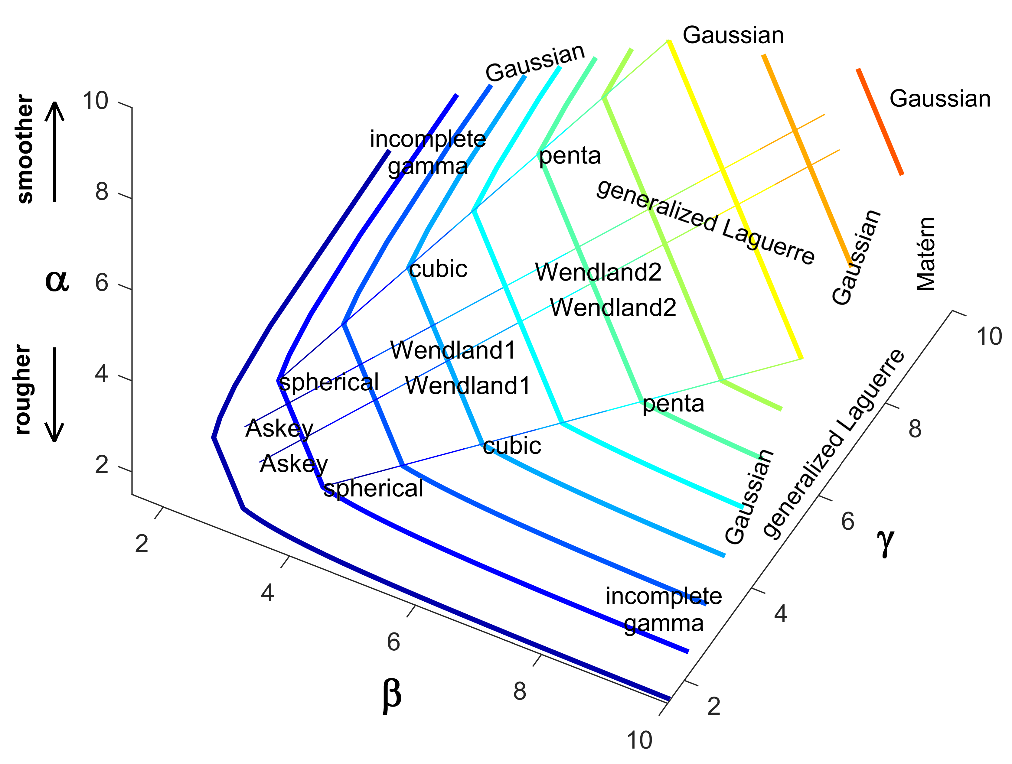
Figure 1: Positioning of common covariance kernels in the parameter space $\mathcal{P}_{d}$ (with, here, $d=3$) of the hypergeometric covariance. The colored lines represent the upper boundary of $\mathcal{P}_{3}$, the color being a function of $\alpha$, from the lowest (blue) to the highest (red) values; the thin lines correspond to the spherical and Askey-Wendland families. The lower boundary of $\mathcal{P}_{3}$ is the white plane $\alpha=\frac{3}{2}$. The greater $\alpha$, the more regular the hypergeometric covariance at the origin.

Appendices

Appendix A Technical definitions and lemmas

Definition 1 (Montée and descente).

For $k\in\mathbb{N}$, $k<d$, the transitive upgrading or montée of order $k$ is the operator $\mathfrak{M}_{k}$ that transforms an isotropic covariance in $\mathbb{R}^{d}$ into a an isotropic covariance in $\mathbb{R}^{d-k}$ with the same radial spectral density (Matheron, , 1965). The reciprocal operator is the transitive downgrading (descente) of order $k$ and is denoted as $\mathfrak{M}_{-k}$.

Definition 2 (Conditionally negative semidefinite matrix).

A $p\times p$ symmetric real-valued matrix $\boldsymbol{A}$ is conditionally negative semidefinite if, for any vector $\boldsymbol{\omega}$ in $\mathbb{R}^{p}$ whose components add to zero, one has $\boldsymbol{\omega}^{\top}\,\boldsymbol{A}\boldsymbol{\omega}\leq 0$.

Example 1.

Examples of conditionally negative semidefinite matrices include the all-ones matrix $\boldsymbol{1}$ or the matrix $\boldsymbol{A}=[a_{ij}]_{i,j=1}^{p}$ with

$$a_{ij}=\frac{\eta_{i}+\eta_{j}}{2}+\psi(\boldsymbol{s}_{i},\boldsymbol{s}_{j}),$$

for any $\eta_{1},\ldots,\eta_{p}$ in $\mathbb{R}$, $\boldsymbol{s}_{1},\ldots,\boldsymbol{s}_{p}$ in $\mathbb{R}^{d}$, and variogram $\psi$ on $\mathbb{R}^{d}\times\mathbb{R}^{d}$ (Matheron, , 1965; Chilès and Delfiner, , 2012). Also, the set of conditionally negative semidefinite matrices is a closed convex cone, so that the product of a conditionally negative semidefinite matrix with a nonnegative constant, the sum of two conditionally negative semidefinite matrices, or the limit of a convergent sequence of conditionally negative semidefinite matrices are still conditionally negative semidefinite.

Lemma 1 (Berg et al., (1984)).

A symmetric real-valued matrix $\boldsymbol{A}=[a_{ij}]_{i,j=1}^{p}$ is conditionally negative semidefinite if and only if $[\exp(-t\,a_{ij})]_{i,j=1}^{p}$ is positive semidefinite for all $t\geq 0$.

Definition 3 (Multiply monotone function).

For $q\in\mathbb{N}$, a $q$-times differentiable function $\varphi$ on $\mathbb{R}_{+}$ is $(q+2)$-times monotone if $(-1)^{k}\varphi^{(k)}$ is nonnegative, nonincreasing and convex for $k=0,\ldots,q$. A $1$-time monotone function is a nonnegative and nonincreasing function on $\mathbb{R}_{+}$ (Williamson, , 1956).

Lemma 2 (Williamson, (1956)).

A $(q+2)$-times monotone function, $q\geq-1$, admits the expression

$$\varphi(x)=\int_{0}^{+\infty}(1-t\,x)_{+}^{q+1}\,\nu(\textnormal{d}t),\qquad x\in\mathbb{R}_{+},$$ (15)

where $\nu$ is a nonnegative measure.

Example 2.

Examples of $(q+2)$-times monotone functions include the truncated power function $x\mapsto b+(1-\frac{x}{a})_{+}^{\eta}$ with $a>0$, $b\geq 0$ and $\eta\geq q+1$, the completely monotone functions, and positive mixtures and products of such functions.

Lemma 3.

Let $q\in\mathbb{N}$, $\alpha,\beta$, $\gamma\in\mathbb{R}_{+}^{*}$ and $\psi_{1}$ a positive function in $\mathbb{R}_{+}$ whose derivative is $(q+1)$-times monotone. Then, the function $\Phi_{1}:\mathbb{R}^{2q+1}\to\mathbb{R}$ defined by

$$\Phi_{1}({\boldsymbol{x}})={}_{1}F_{2}\left(\alpha;\beta,\gamma;-\psi_{1}(\|{\boldsymbol{x}}\|)\right),\quad{\boldsymbol{x}}\in\mathbb{R}^{2q+1},$$ (16)

is a stationary isotropic covariance kernel in $\mathbb{R}^{2q+1}$ if $(\alpha+q+2,\beta+q+2,\gamma+q+2)\in\mathcal{P}_{0}$.

Example 3.

Examples of functions $\psi_{1}$ satisfying the conditions of Lemma 3 include the integrated truncated power function $\psi_{1}(x)=b\,x+c-(1-\frac{x}{a})_{+}^{\eta+1}$ ($a>0$, $b>0$, $c>1$ and $\eta\geq q$) and the Bernstein functions (positive primitives of completely monotone functions), e.g. (Schilling et al., , 2010):

• $\psi_{1}(x)=1+\log\left(1+\frac{x}{b}\right)$ with $b>0$;

• $\psi_{1}(x)=\left(1+b\,x^{\eta}\right)^{\theta}$ with $b>0$, $\eta\in]0,1]$ and $\theta\in]0,1]$;

• $\psi_{1}(x)=1+x\,(x+b)^{-\eta}$ with $b>0$ and $\eta\in]0,1]$.

Lemma 4.

Let $q^{\prime}\in\mathbb{N}$, $\gamma>0$, $x>0$ and $\psi_{2}$ a positive function in $\mathbb{R}_{+}$ upper bounded by $\alpha_{\max}=\frac{2\gamma-1}{4}$ and whose derivative is $(q^{\prime}+1)$-times monotone. Then, the function $\Phi_{2}:\mathbb{R}^{2q^{\prime}+1}\to\mathbb{R}$ defined by

$$\Phi_{2}(\boldsymbol{y})={}_{1}F_{2}\left(\psi_{2}(\|\boldsymbol{y}\|);\psi_{2}(\|\boldsymbol{y}\|)+1,\gamma;-x\right),\quad\boldsymbol{y}\in\mathbb{R}^{2q^{\prime}+1},$$ (17)

is a stationary isotropic covariance kernel in $\mathbb{R}^{2q^{\prime}+1}$.

Lemma 5.

Let $q,q^{\prime}\in\mathbb{N}$, $\gamma>0$, $\psi_{1}$ a positive function in $\mathbb{R}_{+}$ with a $(q+1)$-times monotone derivative, and $\psi_{2}$ a positive function in $\mathbb{R}_{+}$ upper bounded by $\alpha_{\max}=\frac{2\gamma-1}{4}$ and with a $(q^{\prime}+1)$-times monotone derivative. Then, the function $\Phi:\mathbb{R}^{2q+1}\times\mathbb{R}^{2q^{\prime}+1}\to\mathbb{R}$ defined by

$$\Phi(\boldsymbol{x},\boldsymbol{y})=\frac{1}{\psi_{1}(\|\boldsymbol{x}\|)}{}_{1}F_{2}\left(\psi_{2}(\|\boldsymbol{y}\|);\psi_{2}(\|\boldsymbol{y}\|)+1,\gamma;-\psi_{1}(\|\boldsymbol{x}\|)\right),\quad\boldsymbol{x}\in\mathbb{R}^{2q+1},\boldsymbol{y}\in\mathbb{R}^{2q^{\prime}+1},$$ (18)

is positive semidefinite in $\mathbb{R}^{2q+1}\times\mathbb{R}^{2q^{\prime}+1}$ if $(\alpha+q+3,\alpha+q+4,\gamma+q+3)\in\mathcal{P}_{0}$.

Appendix B Proofs

Proof of Theorem 2.

Let $(\alpha,\beta,\gamma)\in\mathcal{P}_{d}$. As the complex extension of the generalized hypergeometric function $x\mapsto{}_{1}F_{2}(\alpha,\beta,\gamma,x)$, $x\in\mathbb{C}$, is an entire function not identically equal to zero, its zeroes (if they exist) are isolated. It follows that there exists an nonempty open interval $I\subseteq\mathbb{R}$ such that ${}_{1}F_{2}(\alpha,\beta,\gamma,x)$ does not vanish, hence is positive, for all $x\in I$. Accordingly, the support of the spectral density (8) contains a nonempty open set of $\mathbb{R}^{d}$, which implies that the associated covariance kernel is positive definite Dolloff et al., (2006). ∎

Proof of Theorem 3.

The claim stems from the fact that $g_{d-k}(\cdot;a,\alpha-\frac{k}{2},\beta-\frac{k}{2},\gamma-\frac{k}{2})$ is the same as $g_{d}(\cdot;a,\alpha,\beta,\gamma)$ and that $(\alpha-\frac{k}{2},\beta-\frac{k}{2},\gamma-\frac{k}{2})\in\mathcal{P}_{d-k}$ as soon as $(\alpha,\beta,\gamma)\in\mathcal{P}_{d}$. ∎

Proof of Theorem 4.

The proof is analog to that of Theorem 3, with the additional restriction to ensure that the extended covariance remains valid in $\mathbb{R}^{d+k}$. ∎

Proof of Theorem 5.

The continuity and differentiability with respect to $r$ stem from the fact that the Gauss hypergeometric function $x\mapsto{}_{2}F_{1}(a_{1},a_{2};b_{1};x)$ with $b_{1}-a_{1}-a_{2}>0$ is continuous on the interval $[0,1]$, equal to $1$ at $x=0$, and infinitely differentiable on $]0,1[$. One deduces the continuity and differentiability with respect to $a$ by noting that, for fixed $\alpha$, $\beta$ and $\gamma$, $g_{d}(r;a,\alpha,\beta,\gamma)$ only depends on $\frac{r}{a}$. Finally, the continuity and differentiability with respect to $\alpha$, $\beta$ and $\gamma$ stem from the fact that the exponential function of base $\left(1-(\frac{r}{a})^{2}\right)_{+}$ and the gamma function are infinitely differentiable wherever they are defined, and the hypergeometric function ${}_{2}F_{1}$ is an entire function of its parameters. ∎

Proof of Theorem 6.

From (10), it is seen that $r\mapsto g_{d}(r;a,\alpha,\beta,\gamma)$ is of the order of $(1-\frac{r}{a})^{\beta+\gamma-\alpha-\frac{d}{2}-1}$ as $r\to a^{-}$, while it is identically zero for $r\to a^{+}$. Hence, this function is $k$ times differentiable (with zero derivatives of order $1,2,\ldots,k$) at $r=a$, if, and only if, $\beta-\alpha+\gamma>k+\frac{d}{2}+1$. ∎

Proof of Theorem 7.

Using formula E.2.3 of Matheron, (1965), one obtains, for $\alpha-\frac{d}{2}\not\in\mathbb{N}$:

$$\begin{split}g_{d}(r;a,\alpha,\beta,\gamma)&={}_{2}F_{1}\left(\frac{d}{2}-\gamma+1,\frac{d}{2}-\beta+1;\frac{d}{2}-\alpha+1;\frac{r^{2}}{a^{2}}\right)\\ &+\frac{\Gamma(\frac{d}{2}-\alpha)\Gamma(\beta-\frac{d}{2})\Gamma(\gamma-\frac{d}{2})}{\Gamma(\alpha-\frac{d}{2})\Gamma(\beta-\alpha)\Gamma(\gamma-\alpha)}\left(\frac{r}{a}\right)^{2\alpha-d}\\ &\times{}_{2}F_{1}\left(\alpha-\beta+1,\alpha-\gamma+1;\alpha-\frac{d}{2}+1;\frac{r^{2}}{a^{2}}\right),\quad 0\leq r<a.\end{split}$$ (19)

The right-hand side of (19) is a power series of $r^{2}$, plus a power series of $r^{2}$ (with a constant nonzero term) multiplied by $r^{2\alpha-d}$. Since $2\alpha-d$ is not an even integer, $r\mapsto g_{d}(r;a,\alpha,\beta,\gamma)$ turns out to be $k$ times differentiable at $r=0$ if, and only if, $\alpha>\frac{k+d}{2}$. If $\alpha-\frac{d}{2}\in\mathbb{N}$, then formula E.2.4 of Matheron, (1965) shows that $r\mapsto g_{d}(r;a,\alpha,\beta,\gamma)$ is a power series of $r^{2}$ plus a power series of $r^{2}$ (with a constant nonzero term) multiplied by $r^{2\alpha-d}\log(\frac{r}{a})$, and the same conclusion prevails: $r\mapsto g_{d}(r;a,\alpha,\beta,\gamma)$ is $k$ times differentiable at $r=0$ if, and only if, $\alpha>\frac{k+d}{2}$. ∎

Proof of Theorem 8.

Using an integral representation of the Gauss hypergeometric function ${}_{2}F_{1}$ (Gradshteyn and Ryzhik, , 2007, formula 9.111), the restriction of the radial function $g_{d}$ on the interval $[0,a]$ can be written as follows:

$$\begin{split}g_{d}(r;a,\alpha,\beta,\gamma)=&\frac{\Gamma(\gamma-\frac{d}{2})}{\Gamma(\gamma-\alpha)\Gamma(\alpha-\frac{d}{2})}\left(1-\frac{r^{2}}{a^{2}}\right)^{\beta-\alpha+\gamma-\frac{d}{2}-1}\\ &\times\int_{0}^{1}t^{\gamma-\alpha-1}(1-t)^{\alpha-\frac{d}{2}-1}\left(1+\frac{t}{1-t}\frac{r^{2}}{a^{2}}\right)^{\alpha-\beta}\text{d}t,\quad r\in[0,a].\end{split}$$ (20)

Accordingly, on $[0,a]$, $r\mapsto g_{d}(r;a,\alpha,\beta,\gamma)$ appears as a beta mixture of powered quadratic functions of the form $r\mapsto(1-\frac{r^{2}}{a^{2}})^{\beta-\alpha+\gamma-\frac{d}{2}-1}$ multiplied by generalized Cauchy covariance functions of the form $r\mapsto(1+\frac{t}{1-t}\frac{r^{2}}{a^{2}})^{\alpha-\beta}$, with $t\in]0,1[$, $a>0$ and $(\alpha,\beta,\gamma)\in\mathcal{P}_{d}$. Since all these functions are nonnegative and decreasing on $[0,a]$, so is $r\mapsto g_{d}(r;a,\alpha,\beta,\gamma)$.

The monotonicity in $r$ implies the monotonicity in $a$, insofar as $g_{d}(r;a,\alpha,\beta,\gamma)$ only depends on $\frac{r}{a}$ for fixed $\alpha$,$\beta$ and $\gamma$.

Consider the integral representation (9) as a function of $r=\|\boldsymbol{h}\|$, $a$, $\alpha$, $\beta$ and $\gamma$. Based on the dominated convergence theorem, this function can be differentiated under the integral sign with respect to parameter $\gamma$, which leads to:

$$\begin{split}\frac{\partial g_{d}(r;a,\alpha,\beta,\gamma)}{\partial\gamma}&=\frac{\Gamma(\beta-\frac{d}{2})}{\Gamma(\alpha-\frac{d}{2})\Gamma(\beta-\alpha)}\\ &\times\int_{0}^{1}t^{\alpha-\gamma}(1-t)_{+}^{\beta-\alpha-1}\left(t-\left(\frac{r}{a}\right)^{2}\right)_{+}^{\gamma-\frac{d}{2}-1}\ln\left(1-\frac{r^{2}}{ta^{2}}\right)_{+}\text{d}t.\end{split}$$

This equation includes the $r=0$ instance, as $\gamma\mapsto g_{d}(1;a,\alpha,\beta,\gamma)$ is identically equal to $1$. The partial derivative is therefore always negative (if $0<r<a$) or zero (if $r=0$ or $r>a$), implying that $\gamma\mapsto g_{d}(r;a,\alpha,\beta,\gamma)$ is decreasing or constant in $\gamma$, respectively. The same result holds by substituting $\beta$ for $\gamma$ owing to the symmetry of the ${}_{2}F_{1}$ function. ∎

Proof of Theorem 9.

For $(\alpha,\beta,\gamma)\in\mathcal{P}_{d}$, the radial part of $\mathfrak{M}_{k}(G_{d}(\cdot,a,\alpha,\beta,\gamma))$ is the Hankel transform of order $d-k$ of $\widetilde{g}_{d}(\cdot,a,\alpha,\beta,\gamma)$. From (3), one has

$$\mathfrak{M}_{k}(G_{d}(\cdot,a,\alpha,\beta,\gamma))=\frac{\zeta_{d}(a,\alpha,\beta,\gamma)}{\zeta_{d-k}(a,\alpha,\beta,\gamma)}G_{d-k}(\cdot,a,\alpha,\beta,\gamma).$$

Since $\mathcal{P}_{d}\subset\mathcal{P}_{d-k}$, it follows that $\mathfrak{M}_{k}(G_{d}(\cdot,a,\alpha,\beta,\gamma))\in\mathcal{G}_{d-k}$, its radial part being

$$\frac{\zeta_{d}(a,\alpha,\beta,\gamma)}{\zeta_{d-k}(a,\alpha,\beta,\gamma)}g_{d-k}(\cdot,a,\alpha,\beta,\gamma)=\frac{\zeta_{d}(a,\alpha,\beta,\gamma)}{\zeta_{d-k}(a,\alpha,\beta,\gamma)}\,g_{d}\left(\cdot,a,\alpha+\frac{k}{2},\beta+\frac{k}{2},\gamma+\frac{k}{2}\right).$$

∎

Proof of Theorem 10.

The proof follows that of Theorem 9. The condition $(\alpha-\frac{k}{2},\beta-\frac{k}{2},\gamma-\frac{k}{2})\in\mathcal{P}_{d+k}$ ensures that the downgraded covariance is positive semidefinite in $\mathbb{R}^{d+k}$, based on Theorem 1. ∎

Proof of Theorem 11.

The proof relies on expansion (19) of the radial function $r\mapsto g_{d}(r;a,\alpha,\beta,\gamma)$, valid for $r\in[0,a]$ and $\alpha-\frac{d}{2}\not\in\mathbb{N}$. Using formulae 5.5.3 and 5.11.12 of Olver et al., (2010), as well as the theorem of dominated convergence to interchange limits and infinite summations, one finds the following asymptotic equivalence:

$$\begin{split}g_{d}(r;a,\alpha,\beta,\gamma)&\sim{}_{0}F_{1}\left(;\frac{d}{2}-\alpha+1;\frac{\beta\gamma r^{2}}{a^{2}}\right)\\ &+\frac{\Gamma(\frac{d}{2}-\alpha)}{\Gamma(\alpha-\frac{d}{2})}\left(\frac{\beta\gamma r^{2}}{a^{2}}\right)^{\alpha-\frac{d}{2}}{}_{0}F_{1}\left(;\alpha-\frac{d}{2}+1;\frac{\beta\gamma r^{2}}{a^{2}}\right),\quad r\leq a,\end{split}$$

as $\beta\to+\infty$ and $\gamma\to+\infty$. The left-hand side can be expressed in terms of modified Bessel functions of the first ($I_{\eta}$) and second ($K_{\eta}$) kinds thanks to formulae 5.5.3, 10.27.4 and 10.39.9 of Olver et al., (2010), which finally yields:

$$\begin{split}g_{d}(r;a,\alpha,\beta,\gamma)&\sim\Gamma\left(\frac{d}{2}-\alpha+1\right)\left(\frac{\sqrt{\beta\gamma}r}{a}\right)^{\alpha-\frac{d}{2}}I_{\frac{d}{2}-\alpha}\left(\frac{2\sqrt{\beta\gamma}r}{a}\right)\\ &+\frac{\Gamma(\frac{d}{2}-\alpha)}{\Gamma(\alpha-\frac{d}{2})}\Gamma\left(\alpha-\frac{d}{2}+1\right)\left(\frac{\sqrt{\beta\gamma}r}{a}\right)^{\alpha-\frac{d}{2}}I_{\alpha-\frac{d}{2}}\left(\frac{2\sqrt{\beta\gamma}r}{a}\right)\\ &=\frac{2}{\Gamma\left(\alpha-\frac{d}{2}\right)}\left(\frac{\sqrt{\beta\gamma}r}{a}\right)^{\alpha-\frac{d}{2}}K_{\alpha-\frac{d}{2}}\left(\frac{2\sqrt{\beta\gamma}r}{a}\right),\quad r\leq a.\end{split}$$ (21)

Accordingly, $g_{d}(\cdot;a,\alpha,\beta,\gamma)$ tends pointwise to the radial part of the Matérn covariance (12) by letting $\beta$ and $\gamma$ tend to infinity and $a$ be asymptotically equivalent to $2b\sqrt{\beta\gamma}$. In particular, since $a$ tends to infinity, the pointwise convergence is true for any $r\geq 0$. It is also true if $\alpha-\frac{d}{2}\in\mathbb{N}$, as it suffices to consider the asymptotic equivalence (21) with $\alpha-\delta-\frac{d}{2}$ and $\delta>0$ and then to let $\delta$ tend to zero, both the Gauss hypergeometric and Matérn covariances being continuous with respect to the parameter $\alpha$. Note that the conditions of Theorem 1 are fulfilled when $\alpha$ is fixed and greater than $\frac{d}{2}$ and $\beta$ and $\gamma$ become infinitely large, so that $g_{d}(\cdot;a,\alpha,\beta,\gamma)$ in (21) is the radial part of a valid covariance kernel. Finally, because $g_{d}(\cdot;a,\alpha,\beta,\gamma)$ is a decreasing function on any compact segment of $\mathbb{R}_{+}$ for sufficiently large $a$ and $\beta$ or $\gamma$ (Theorem 8) and the limit function (the radial part of the Matérn covariance (12)) is continuous on $\mathbb{R}_{+}$, Dini’s second theorem implies that the pointwise convergence is actually uniform on any compact segment of $\mathbb{R}_{+}$. In turn, since all the functions are lower bounded by zero, uniform convergence on a compact segment of $\mathbb{R}_{+}$ implies uniform convergence on $\mathbb{R}_{+}$. ∎

The proofs of Theorems 12 to 16 use of the same argument as above to identify pointwise convergence with uniform convergence. This argument will be omitted for the sake of brevity.

Proof of Theorem 12.

The starting point is the expansion (19) of $g_{d}(\cdot;a,\alpha,\beta,\gamma)$ in $[0,a]$. Using formulae 5.5.3 and 5.11.12 of Olver et al., (2010) and the dominated convergence theorem to interchange limits and infinite summations, one finds the following asymptotic equivalence as $\gamma$ tends to infinity:

$$\begin{split}g_{d}&\left(r;a,\alpha,\beta,\gamma\right)\sim{}_{1}F_{1}\left(\frac{d}{2}-\beta+1;\frac{d}{2}-\alpha+1;-\frac{\gamma\,r^{2}}{a^{2}}\right)\\ &+{}_{1}F_{1}\left(\alpha-\beta+1;\alpha-\frac{d}{2}+1;-\frac{\gamma\,r^{2}}{a^{2}}\right)\frac{\Gamma(\frac{d}{2}-\alpha)\Gamma(\beta-\frac{d}{2})}{\Gamma(\alpha-\frac{d}{2})\Gamma(\beta-\alpha)}\left(\frac{\gamma\,r^{2}}{a^{2}}\right)^{\alpha-\frac{d}{2}},\quad 0\leq r<a.\end{split}$$ (22)

Using formula D.8 of Matheron, (1965) and letting $a\to+\infty$ such that $\frac{a}{\sqrt{\gamma}}\to b>0$ yields the claim. ∎

Proof of Theorem 13.

The proof relies on (22) and formulae 5.5.3 and 13.2.42 of Olver et al., (2010). ∎

Proof of Theorem 14.

The proof relies on (22) and formulae 8.2.3, 8.2.4, 8.5.1 and 13.6.3 of Olver et al., (2010). ∎

Proof of Theorem 15.

The proof follows from Theorem 11 and the fact that the Matérn covariance (12) with scale parameter $b/(2\sqrt{\alpha})$ and smoothness parameter $\alpha$ tends to the Gaussian covariance (13) as $\alpha\to+\infty$. Following Chernih et al., (2014), the convergence can also be shown by noting that the spectral density (8) of the Gauss hypergeometric covariance is asymptotically equivalent to

$$\begin{split}\widetilde{G}_{d}({\boldsymbol{u}};a,\alpha,\beta,\gamma)&\sim\left(\frac{\pi a^{2}\alpha}{\beta\gamma}\right)^{\frac{d}{2}}\,\sum_{n=0}^{+\infty}\frac{1}{n!}\left(-\frac{\alpha(\pi a\|{\boldsymbol{u}}\|)^{2}}{\beta\gamma}\right)^{n}\\ &=\left(\frac{\pi a^{2}\alpha}{\beta\gamma}\right)^{\frac{d}{2}}\,\exp\left(-\frac{\alpha(\pi a\|{\boldsymbol{u}}\|)^{2}}{\beta\gamma}\right),\quad{\boldsymbol{u}}\in\mathbb{R}^{d},\end{split}$$

as $\alpha\to+\infty$, $\beta\to+\infty$ and $\gamma\to+\infty$. If, furthermore, $a\to+\infty$ such that $a\sqrt{\frac{\alpha}{\beta\gamma}}\to b>0$, then one obtains:

$$\widetilde{G}_{d}({\boldsymbol{u}};a,\alpha,\beta,\gamma)\sim\pi^{\frac{d}{2}}b^{d}\,\exp\left(-(\pi b\|{\boldsymbol{u}}\|)^{2}\right),\quad{\boldsymbol{u}}\in\mathbb{R}^{d},$$

which coincides with the spectral density of the Gaussian covariance (13) (Arroyo and Emery, , 2020; Lantuéjoul, , 2002). ∎

Proof of Theorem 16.

The proof follows from the asymptotic equivalence (22) for $\gamma$ tending to infinity. As $\beta$ tends to $\alpha$ and $a$ tends to infinity in such a way that $\frac{a}{\sqrt{\gamma}}$ tends to $b>0$, the first term in the right-hand side of (22) tends to $\exp(-r^{2}/b^{2})$ and the second term to zero. ∎

Proof of Lemma 3.

One has $\Phi_{1}({\boldsymbol{x}})=\varphi_{1}\circ\psi_{1}(\|\boldsymbol{x}\|)$, where $\varphi_{1}:x\mapsto{}_{1}F_{2}\left(\alpha;\beta,\gamma;-x\right)$ is an infinitely differentiable function on $\mathbb{R}_{+}$, with (Olver et al., , 2010, formula 16.3.1)

$$(-1)^{k}\frac{\partial^{k}\varphi_{1}}{\partial x^{k}}(x)=\frac{\Gamma(\alpha+k)\Gamma(\beta)\Gamma(\gamma)}{\Gamma(\alpha)\Gamma(\beta+k)\Gamma(\gamma+k)}{}_{1}F_{2}\left(\alpha+k;\beta+k,\gamma+k;-x\right),\quad x\in\mathbb{R}_{+},k\in\mathbb{N}.$$

If $(\alpha+q+2,\beta+q+2,\gamma+q+2)\in\mathcal{P}_{0}$, then, for any $k=0,\ldots,q+2$, $(\alpha+k,\beta+k,\gamma+k)\in\mathcal{P}_{0}$ and $(-1)^{k}\frac{\partial^{k}\varphi_{1}}{\partial x^{k}}$ is nonnegative on $\mathbb{R}_{+}$, hence $\varphi_{1}$ is $(q+2)$-times monotone. Since $\psi_{1}$ is positive and has a $(q+1)$-times monotone derivative, the composite function $\varphi_{1}\circ\psi_{1}$ is $(q+2)$-times monotone (Gneiting, , 1999, proposition 4.5). The fact that this composite function is continuous implies that $\Phi_{1}$ is positive semidefinite in $\mathbb{R}^{2q+1}$ (Askey, , 1973; Micchelli, , 1986; Gneiting, , 1999, criterion 1.3). ∎

Proof of Lemma 4.

$\Phi_{2}({\boldsymbol{y}})=\varphi_{2}\circ\psi_{2}(\|\boldsymbol{y}\|)$, where $\varphi_{2}:\alpha\mapsto{}_{1}F_{2}\left(\alpha;\alpha+1,\gamma;-x\right)$ is a nonnegative function on $[0,\alpha_{\max}]$, insofar as $(\alpha,\alpha+1,\gamma)\in\mathcal{P}_{0}$ as soon as $\alpha\leq\alpha_{\max}$. This function is infinitely differentiable; for $k\in\mathbb{N}^{*}$, its $k$-th derivative, obtained with a term-by-term differentiation of (1), is

$$\begin{split}\frac{\partial^{k}\varphi_{2}}{\partial\alpha^{k}}(\alpha)&=\sum_{n=1}^{+\infty}\frac{(-1)^{k-1}k!\,n\,\Gamma(\gamma)}{n!(\alpha+n)^{k+1}\Gamma(\gamma+n)}\left(-x\right)^{n}\\ &=\frac{(-1)^{k}k!\,x}{(\alpha+1)^{k+1}\gamma}\sum_{n=0}^{+\infty}\frac{(\alpha+1)^{k+1}\Gamma(\gamma+1)}{n!(\alpha+1+n)^{k+1}\Gamma(\gamma+1+n)}\left(-x\right)^{n}\\ &=\frac{(-1)^{k}k!\,x}{(\alpha+1)^{k+1}\gamma}\,{}_{k+1}F_{k+2}\left(\alpha+1,\ldots,\alpha+1;\alpha+2,\ldots,\alpha+2,\gamma+1;-x\right).\end{split}$$ (23)

If $\alpha\in[0,\alpha_{\max}]$, then $(\alpha+1,\alpha+2,\gamma+1)\in\mathcal{P}_{0}$ and ${}_{k+1}F_{k+2}(\alpha+1,\ldots,\alpha+1;\alpha+2,\ldots,\alpha+2,\gamma+1;-x)$ is nonnegative, as a beta mixture of nonnegative ${}_{1}F_{2}$ functions (Olver et al., , 2010, formula 16.5.2), which implies that $\varphi_{2}$ is completely monotone on $[0,\alpha_{\max}]$. Since $\psi_{2}$ is positive with values in $[0,\alpha_{\max}]$ and has a $(q^{\prime}+1)$-times monotone derivative, the composition $\varphi_{2}\circ\psi_{2}$ is $(q^{\prime}+2)$-times monotone on $\mathbb{R}_{+}$. As it is continuous, this entails that $\Phi_{2}$ is a positive semidefinite in $\mathbb{R}^{2q^{\prime}+1}$ (Micchelli, , 1986). ∎

Proof of Lemma 5.

Let introduce $\Phi(\boldsymbol{x},\boldsymbol{y})=\varphi(\psi_{1}(\|\boldsymbol{x}\|),\psi_{2}(\|\boldsymbol{y}\|))$, where $\varphi:(x,\alpha)\mapsto\frac{1}{x}\,{}_{1}F_{2}\left(\alpha;\alpha+1,\gamma;-x\right)$ is nonnegative and infinitely differentiable on $\mathbb{R}_{+}^{*}\times[0,\alpha_{\max}]$. From (23), it comes, for $k,k^{\prime}\in\mathbb{N}$:

$$\begin{split}&\frac{\partial^{k+k^{\prime}}\varphi}{\partial x^{k}\,\partial\alpha^{k^{\prime}}}(x,\alpha)=\sum_{n=0}^{+\infty}\frac{(-1)^{k+k^{\prime}}k^{\prime}!\,\Gamma(\gamma)}{\Gamma(n+1)(\alpha+n+k+1)^{k^{\prime}+1}\Gamma(\gamma+n+k+1)}\left(-x\right)^{n}\\ &=\frac{(-1)^{k+k^{\prime}}k^{\prime}!\,\Gamma(\gamma)}{(\alpha+k+1)^{k^{\prime}+1}\Gamma(\gamma+k+1)}\\ &\quad\times{}_{k^{\prime}+1}F_{k^{\prime}+2}\left(\alpha+k+1,\ldots,\alpha+k+1;\alpha+k+2,\ldots,\alpha+k+2,\gamma+k+1;-x\right).\end{split}$$

If $(\alpha+q+3,\alpha+q+4,\gamma+q+3)\in\mathcal{P}_{0}$, then, for any $k=0,\ldots,q+2$, $(\alpha+k+1,\alpha+k+2,\gamma+k+1)\in\mathcal{P}_{0}$ and the hypergeometric term ${}_{k^{\prime}+1}F_{k^{\prime}+2}$ is nonnegative, as a beta mixture of nonnegative ${}_{1}F_{2}$ terms. Under this condition, $(-1)^{k+k^{\prime}}\frac{\partial^{k+k^{\prime}}\varphi}{\partial x^{k}\,\partial\alpha^{k^{\prime}}}$ is nonnegative for $k=0,\ldots,q+2$ and any $k^{\prime}\in\mathbb{N}$. Accordingly, $\varphi$ is a bivariate multiply monotone function of order $(q+2,q^{\prime}+2)$, and so is the composite function $\varphi(\psi_{1},\psi_{2})$ (Gneiting, , 1999, proposition 4.5). Arguments in Williamson, (1956) generalized to functions of two variables imply that $\varphi(\psi_{1},\psi_{2})$ is a mixture of products of truncated power functions of the form (15) (one function of $x$ with power exponent $q+1$ times one function of $\alpha$ with power exponent $q^{\prime}+1$) and is the radial part of a product covariance kernel in $\mathbb{R}^{2q+1}\times\mathbb{R}^{2q^{\prime}+1}$. ∎

Proof of Theorem 17.

We start proving (1). Conditions (i), (ii) and (v) imply the existence of a spectral density associated with each direct or cross covariance (Theorem 1). Based on Cramér’s criterion (Cramér, , 1940; Chilès and Delfiner, , 2012), $\boldsymbol{\widetilde{G}}_{d}(\cdot;a\boldsymbol{1},\alpha\boldsymbol{1},\boldsymbol{\beta},\boldsymbol{\gamma},\boldsymbol{\rho})$ is a valid matrix-valued spectral density function if, and only if, $\boldsymbol{\widetilde{G}}_{d}(\boldsymbol{u};a\boldsymbol{1},\alpha\boldsymbol{1},\boldsymbol{\beta},\boldsymbol{\gamma},\boldsymbol{\rho})$ is positive semidefinite for any vector $\boldsymbol{u}\in\mathbb{R}^{d}$. The key of the proof is to expand this matrix as a positive mixture of positive semidefinite matrices. Such an expansion rests on the following identity, which can be obtained by a term-by-term integration of the infinite series (1) defining the generalized hypergeometric function ${}_{1}F_{2}$ along with formula 3.251.1 of Gradshteyn and Ryzhik, (2007):

$$\begin{split}\int_{0}^{1}&\int_{0}^{1}{}_{1}F_{2}\left(\alpha;\beta,\gamma;-t_{1}t_{2}(a\,x)^{2}\right)t_{1}^{\beta-1}(1-t_{1})^{\beta_{ij}-\beta-1}t_{2}^{\gamma-1}(1-t_{2})^{\gamma_{ij}-\gamma-1}\text{d}t_{1}\text{d}t_{2}\\ &=\frac{\Gamma(\beta)\Gamma(\beta_{ij}-\beta)\Gamma(\gamma)\Gamma(\gamma_{ij}-\gamma)}{\Gamma(\beta_{ij})\Gamma(\gamma_{ij})}{}_{1}F_{2}\left(\alpha;\beta_{ij},\gamma_{ij};-(a\,x)^{2}\right),\end{split}$$ (24)

for $x\geq 0,a>0,\alpha>0,\beta_{ij}>\beta>0$ and $\gamma_{ij}>\gamma>0$. Accordingly, for $\boldsymbol{u}\in\mathbb{R}^{d}$:

$$\begin{split}&{\widetilde{\boldsymbol{G}}}_{d}(\boldsymbol{u};{a}\boldsymbol{1},{\alpha}\boldsymbol{1},\boldsymbol{\beta},\boldsymbol{\gamma},\boldsymbol{\rho})=\frac{\pi^{\frac{d}{2}}a^{d}\Gamma(\alpha)\Gamma(\boldsymbol{\beta}-\frac{d}{2})\Gamma(\boldsymbol{\gamma}-\frac{d}{2})\boldsymbol{\rho}}{\Gamma(\alpha-\frac{d}{2})\Gamma(\beta)\Gamma(\boldsymbol{\beta}-\beta)\Gamma(\gamma)\Gamma(\boldsymbol{\gamma}-\gamma)}\\ &\times\int_{0}^{1}\int_{0}^{1}{}_{1}F_{2}\left(\alpha;\beta,\gamma;-{t_{1}\,t_{2}(\pi a\|\boldsymbol{u}\|)^{2}}\right)t_{1}^{\beta-1}(1-t_{1})^{\boldsymbol{\beta}-\beta-1}t_{2}^{\gamma-1}(1-t_{2})^{\boldsymbol{\gamma}-\gamma-1}\text{d}t_{1}\text{d}t_{2},\end{split}$$

with the products, quotients and powers taken element-wise. ${}_{1}F_{2}\left(\alpha;\beta,\gamma;-{t_{1}t_{2}(\pi a\|\boldsymbol{u}\|)^{2}}\right)$ is nonnegative for any $t_{1},t_{2}\in[0,1]$ under Condition (vi) (Cho et al., , 2020). Under Conditions (iii) and (iv), $(1-t_{1})^{\boldsymbol{\beta}}$ and $(1-t_{2})^{\boldsymbol{\gamma}}$ are positive semidefinite matrices (Lemma 1). Along with Condition (vii), ${\widetilde{\boldsymbol{G}}}_{d}(\boldsymbol{u};a\boldsymbol{1},\alpha\boldsymbol{1},\boldsymbol{\beta},\boldsymbol{\gamma},\boldsymbol{\rho})$ is positive semidefinite for any $\boldsymbol{u}$ in $\mathbb{R}^{d}$, as the elewent-wise product of positive semidefinite matrices, which completes the proof for (1).

We now prove (2). Under Condition (vi), the generalized hypergeometric function ${}_{1}F_{2}(\alpha;\beta,\gamma,x)$ is positive and increasing in $x$ on $\mathbb{R}$ (Olver et al., , 2010, formula 16.3.1). Therefore, if $\boldsymbol{a}$ fulfills Condition (i), $[{}_{1}F_{2}\left(\alpha;\beta,\gamma;-t_{1}t_{2}(\,a_{ij}\,x)^{2}\right)]_{i,j=1}^{p}$ is positive semidefinite, as the sum of a min matrix with positive entries (Horn and Johnson, , 2013, problem 7.1.P18) and a diagonal matrix with nonnegative entries. The proof of (1) can then be adapted in a straightforward manner, by substituting such a positive semidefinite matrix for the positive scalar ${}_{1}F_{2}\left(\alpha;\beta,\gamma;-t_{1}t_{2}(\,a\,x)^{2}\right)$.

The proof of (3) follows that of (2) and relies on the fact that, under Conditions (i) and (vi), the matrix $[{}_{1}F_{2}\left(\alpha;\beta,\gamma;-t_{1}t_{2}(\,a_{ij}\,x)^{2}\right)]_{i,j=1}^{p}$ is positive semidefinite for any $t_{1}$, $t_{2}$ and $x$ (Lemma 3).

The proof of (4) is similar to that of (1), with (24) replaced by

$$\begin{split}\int_{0}^{1}&\int_{0}^{1}{}_{1}F_{2}\left(\alpha_{ij};\alpha_{ij}+1,\gamma;-t_{1}t_{2}(a_{ij}\,x)^{2}\right)t_{1}^{\alpha_{ij}}(1-t_{1})^{\beta_{ij}-\alpha_{ij}-2}t_{2}^{\gamma-1}(1-t_{2})^{\gamma_{ij}-\gamma-1}\text{d}t_{1}\text{d}t_{2}\\ &=\frac{\Gamma(\alpha_{ij}+1)\Gamma(\beta_{ij}-\alpha_{ij}-1)\Gamma(\gamma)\Gamma(\gamma_{ij}-\gamma)}{\Gamma(\beta_{ij})\Gamma(\gamma_{ij})}{}_{1}F_{2}\left(\alpha_{ij};\beta_{ij},\gamma_{ij};-(a_{ij}\,x)^{2}\right),\end{split}$$

for $x\geq 0,a_{ij}>0,\beta_{ij}-1>\alpha_{ij}>0$ and $\gamma_{ij}>\gamma>0$ for $i,j$ in $[1,\ldots,p]$. Under Condition (ii), the composite function $t\mapsto\exp(-x(\psi_{2}(t)-\psi_{2}(0)))$ is $(q^{\prime}+2)$-times monotone (Gneiting, , 1999, proposition 4.5), hence it is a mixture of truncated power functions of the form (15) and is the radial part of a positive semidefinite function in $\mathbb{R}^{2q^{\prime}+1}$ for any $x>0$. A classical result by Schoenberg, (1938) states that $\boldsymbol{x}\mapsto\psi_{2}(\|\boldsymbol{x}\|)-\psi_{2}(0)$ is a variogram in $\mathbb{R}^{2q^{\prime}+1}$, so $\boldsymbol{\alpha}$ is conditionally negative semidefinite (Example 1) and $[t_{1}^{\alpha_{ij}}]_{i,j=1}^{p}$ is positive semidefinite for any $t_{1}\in[0,1]$ (Lemma 1). Under Conditions (iii) and (iv), $[(1-t_{1})^{\beta_{ij}-\alpha_{ij}}]_{i,j=1}^{p}$ and $[(1-t_{2})^{\gamma_{ij}}]_{i,j=1}^{p}$ are positive semidefinite for any $t_{1},t_{2}\in[0,1]$ (Lemma 1). Under Condition (ii), $[{}_{1}F_{2}(\alpha_{ij};\alpha_{ij}+1,\gamma;-t_{1}t_{2}(a\,x)^{2})]_{i,j=1}^{p}$ is also positive semidefinite for any $t_{1},t_{2}\in[0,1]$, $a>0$, $x>0$ (Lemma 4). As $(\alpha_{ij}+1,\alpha_{ij}+2,\gamma+1)\in\mathcal{P}_{0}$, the generic entry of this matrix decreases with $a$ (Olver et al., , 2010, formula 16.3.1), hence the matrix $[{}_{1}F_{2}(\alpha_{ij};\alpha_{ij}+1,\gamma;-t_{1}t_{2}(a_{ij}\,x)^{2})]_{i,j=1}^{p}$ has increased diagonal entries and is still positive semidefinite. Finally, Condition (v) and Schur’s product theorem imply that ${\widetilde{\boldsymbol{G}}}_{d}(\boldsymbol{u};\boldsymbol{a},\boldsymbol{\alpha},\boldsymbol{\beta},\boldsymbol{\gamma},\boldsymbol{\rho})$ is positive semidefinite for any $\boldsymbol{u}$ in $\mathbb{R}^{d}$, as the elewent-wise product of positive semidefinite matrices, which completes the proof of (4).

The proof of (5) follows the same line of reasoning as that of (4). The positive semidefiniteness of $[a_{ij}^{-2}\,{}_{1}F_{2}(\alpha_{ij};\alpha_{ij}+1,\gamma;-t_{1}t_{2}(a_{ij}\,x)^{2})]_{i,j=1}^{p}$ now stems from Conditions (i), (ii) and (v) together with Lemma 5.

∎

References

• Ahmed, (2007) Ahmed, S. (2007). Application of geostatistics in hydrosciences. In Thangarajan, M., editor, Groundwater, pages 78–111, Dordrecht. Springer.
• Alabert, (1987) Alabert, F. (1987). The practice of fast conditional simulations through the lu decomposition of the covariance matrix. Mathematical Geology, 19(5):369–386.
• Apanasovich et al., (2012) Apanasovich, T. V., Genton, M. G., and Sun, Y. (2012). A valid Matérn class of cross-covariance functions for multivariate random fields with any number of components. Journal of the American Statistical Association, 107(497):180–193.
• Arroyo and Emery, (2020) Arroyo, D. and Emery, X. (2020). Algorithm 1013: An R implementation of a continuous spectral algorithm for simulating vector gaussian random fields in Euclidean spaces. ACM Transactions on Mathematical software, in press.
• Arroyo et al., (2012) Arroyo, D., Emery, X., and Peláez, M. (2012). An enhanced gibbs sampler algorithm for non-conditional simulation of gaussian random vectors. Computers & Geosciences, 46:138–148.
• Askey, (1973) Askey, R. (1973). Radial characteristic functions. Technical Report No. 1262, Mathematics Research Center, University of Wisconsin-Madison.
• Berg et al., (1984) Berg, C., Christensen, J. P. R., and Ressel, P. (1984). Harmonic Analysis on Semigroups: Theory of Positive Definite and Related Functions. Springer-Verlag.
• Bevilacqua et al., (2020) Bevilacqua, M., Caamaño Carrillo, C., and Porcu, E. (2020). Unifying compactly supported and Matérn covariance functions in spatial statistics. arXiv:2008.02904v1 [math.ST].
• Bevilacqua et al., (2019) Bevilacqua, M., Faouzi, T., Furrer, R., and Porcu, E. (2019). Estimation and prediction using generalized wendland covariance functions under fixed domain asymptotics. Annals of Statistics, 47(2):828–856.
• Buhmann, (1998) Buhmann, M. (1998). Radial functions on compact support. Proceedings of the Edinburgh Mathematical Society, 41:41–46.
• Buhmann, (2001) Buhmann, M. (2001). A new class of radial basis functions with compact support. Mathematics of Computation, 70(233):307–318.
• Chernih et al., (2014) Chernih, A., Sloan, I. H., and Womersley, R. S. (2014). Wendland functions with increasing smoothness converge to a gaussian. Advances in Computational Mathematics, 40(1):185–200.
• Chilès and Delfiner, (2012) Chilès, J.-P. and Delfiner, P. (2012). Geostatistics: Modeling Spatial Uncertainty. John Wiley & Sons, New York.
• Cho et al., (2020) Cho, Y.-K., Chung, S.-Y., and Yun, H. (2020). Rational extension of the Newton diagram for the positivity of ${}_{1}{F}_{2}$ hypergeometric functions and Askey–Szegö problem. Constructive Approximation, 51(1):49–72.
• Cho and Yun, (2018) Cho, Y.-K. and Yun, H. (2018). Newton diagram of positivity for ${}_{1}{F}_{2}$ generalized hypergeometric functions. Integral Transforms and Special Functions, 29(7):527–542.
• Cramér, (1940) Cramér, H. (1940). On the theory of stationary random processes. Annals of Mathematics, 41(1):215–230.
• Cressie, (1993) Cressie, N. A. (1993). Statistics for Spatial Data. Wiley.
• Daley et al., (2015) Daley, D. J., Porcu, E., and Bevilacqua, M. (2015). Classes of compactly supported covariance functions for multivariate random fields. Stochastic Environmental Research and Risk Assessment, 29(4):1249–1263.
• Davis, (1987) Davis, M. (1987). Production of conditional simulations via the LU triangular decomposition of the covariance matrix. Mathematical Geology, 19(2):91–98.
• Dietrich and Newsam, (1993) Dietrich, C. and Newsam, G. (1993). A fast and exact method for multidimensional gaussian stochastic simulations. Water Resources Research, 19:2961–2969.
• Dolloff et al., (2006) Dolloff, J., Lofy, B., Sussman, A., and Taylor, C. (2006). Strictly positive definite correlation functions. In Kadar, I., editor, Signal Processing, Sensor Fusion, and Target Recognition XV, volume 6235, pages 1–18, Bellingham. SPIE.
• Emery et al., (2016) Emery, X., Arroyo, D., and Porcu, E. (2016). An improved spectral turning-bands algorithm for simulating stationary vector Gaussian random fields. Stochastic Environmental Research and Risk Assessment, 30(7):1863–1873.
• Emery and Séguret, (2020) Emery, X. and Séguret, S. (2020). Geostatistics for the Mining Industry. CRC Press, Boca Raton.
• Erdélyi, (1953) Erdélyi, A. (1953). Higher Transcendental Functions. McGraw-Hill.
• Furrer et al., (2006) Furrer, R., Genton, M. G., and Nychka, D. (2006). Covariance tapering for interpolation of large spatial datasets. Journal of Computational and Graphical Statistics, 15(3):502–523.
• Galassi and Gough, (2009) Galassi, M. and Gough, B. (2009). GNU Scientific Library: Reference Manual. GNU manual. Network Theory.
• Galli and Gao, (2001) Galli, A. and Gao, H. (2001). Rate of convergence of the Gibbs sampler in the Gaussian case. Mathematical Geology, 33(6):653–677.
• Gasper, (1975) Gasper, G. (1975). Positivity and special functions. In Askey, R., editor, Theory and Application of Special Functions, pages 375–433, New York. Academic Press.
• Gneiting, (1999) Gneiting, T. (1999). Radial positive definite functions generated by Euclid’s hat. Journal of Multivariate Analysis, 69(1):88–119.
• Gneiting, (2002) Gneiting, T. (2002). Compactly supported correlation functions. Journal of Multivariate Analysis, 83(2):493–508.
• Gneiting et al., (2010) Gneiting, T., Kleiber, W., and Schlather, M. (2010). Matérn cross-covariance functions for multivariate random fields. Journal of the American Statistical Association, 105:1167–1177.
• Gradshteyn and Ryzhik, (2007) Gradshteyn, I. and Ryzhik, I. (2007). Table of Integrals, Series, and Products. Amsterdam: Academic Press.
• Hohn, (1999) Hohn, M. (1999). Geostatistics and Petroleum Geology. Kluwer Academic, Dordrecht.
• Horn and Johnson, (2013) Horn, R. A. and Johnson, C. R. (2013). Matrix Analysis. Cambridge University Press, Cambridge, 2nd. edition edition.
• Hubbert, (2012) Hubbert, S. (2012). Closed form representations for a class of compactly supported radial basis functions. Advances in Computational Mathematics, 36(1):115–136.
• Johansson, (2017) Johansson, F. (2017). Arb: Efficient arbitrary-precision midpoint-radius interval arithmetic. IEEE Transactions on Computers, 66(8):1281–1292.
• Johansson, (2019) Johansson, F. (2019). Computing hypergeometric functions rigorously. ACM Transactions on Mathematical Software, 45(3):30.
• Kaufman et al., (2008) Kaufman, C. G., Schervish, M. J., and Nychka, D. W. (2008). Covariance tapering for likelihood-based estimation in large spatial data sets. Journal of the American Statistical Association, 103(484):1545–1555.
• Lantuéjoul, (2002) Lantuéjoul, C. (2002). Geostatistical Simulation: Models and Algorithms. Springer-Verlag, Berlin, 2nd. edition edition.
• Lantuéjoul and Desassis, (2012) Lantuéjoul, C. and Desassis, N. (2012). Simulation of a Gaussian random vector: a propagative version of the Gibbs sampler. In 9th International Geostatistics Congress, Oslo. Available at http://geostats2012.nr.no/pdfs/1747181.pdf.
• Matérn, (1986) Matérn, B. (1986). Spatial Variation — Stochastic Models and Their Application to Some Problems in Forest Surveys and Other Sampling Investigations. Springer.
• Matheron, (1965) Matheron, G. (1965). Les Variables Régionalisées et leur Estimation. Masson.
• Micchelli, (1986) Micchelli, C. A. (1986). Interpolation of scattered data: distance matrices and conditionally positive definite functions. Constructive Approximation, 2:11–22.
• Olver et al., (2010) Olver, F. W., Lozier, D. W., Boisvert, R. F., and Clark, C. W. (2010). NIST handbook of mathematical functions hardback and CD-ROM. Cambridge university press.
• Pardo-Igúzquiza and Chica-Olmo, (1993) Pardo-Igúzquiza, E. and Chica-Olmo, M. (1993). The fourier integral method: an efficient spectral method for simulation of random fields. Mathematical Geology, 25(2):177–217.
• Pearson et al., (2017) Pearson, J. W., Olver, S., and Porter, M. A. (2017). Numerical methods for the computation of the confluent and Gauss hypergeometric functions. Numerical Algorithms, 74(3):821–866.
• Porcu et al., (2013) Porcu, E., Daley, D. J., Buhmann, M., and Bevilacqua, M. (2013). Radial basis functions with compact support for multivariate geostatistics. Stochastic Environmental Research and Risk Assessment, 27(4):909–922.
• Porcu and Zastavnyi, (2014) Porcu, E. and Zastavnyi, V. (2014). Generalized Askey functions and their walks through dimensions. Expositiones Mathematicæ, 32(2):169–174.
• Schaback, (2011) Schaback, R. (2011). The missing Wendland functions. Advances in Computational Mathematics, 34(1):67–81.
• Schilling et al., (2010) Schilling, R., Song, R., and Vondraček, Z. (2010). Bernstein Functions. De Gruyter, Berlin.
• Schoenberg, (1938) Schoenberg, I. (1938). Metric spaces and completely monotone functions. Annals of Mathematics, 39(4):811–831.
• Shinozuka, (1971) Shinozuka, M. (1971). Simulation of multivariate and multidimensional random processes. The Journal of the Acoustical Society of America, 49(1B):357–367.
• Stein and Weiss, (1971) Stein, E. and Weiss, G. (1971). Introduction to Fourier Analysis in Euclidean Spaces. Princeton University Press, Princeton.
• Wackernagel, (2003) Wackernagel, H. (2003). Multivariate Geostatistics: an Introduction with Applications. Springer.
• Webster and Oliver, (2007) Webster, R. and Oliver, M. A. (2007). Geostatistics for Environmental Scientists. Wiley, New York.
• Wendland, (1995) Wendland, H. (1995). Piecewise polynomial, positive definite and compactly supported radial functions of minimal degree. Advances in Computational Mathematics, 4(1):389–396.
• Williamson, (1956) Williamson, R. (1956). Multiply monotone functions and their Laplace transforms. Duke Mathematical Journal, 23(2):189–207.
• Wood and Chan, (1994) Wood, A. T. and Chan, G. (1994). Simulation of stationary Gaussian processes in $[0,1]^{d}$. Journal of Computational and Graphical Statistics, 3(4):409–432.
• Zastavnyi, (2006) Zastavnyi, V. (2006). On some properties of Buhmann functions. Ukrainian Mathematical Journal, 58(8):1184.