Spectroscopic study of CEMP-(s & r/s) stars

Abstract

Context. The origin of the enhanced abundances of both s- and r-process elements observed in a subclass of carbon-enhanced metal-poor (CEMP) stars, denoted CEMP-r/s stars, still remains poorly understood. The i-process nucleosynthesis has been suggested as one of the most promising mechanisms for the origin of these stars.

Aims. Our aim is to better understand the chemical signatures and formation mechanism(s) of five previously claimed potential CH star candidates HE 0017+0055, HE 2144$-$1832, HE 2339$-$0837, HD 145777, and CD$-$27 14351 through a detailed systematic follow-up spectroscopic study based on high-resolution spectra.

Methods. The stellar atmospheric parameters, the effective temperature T_eff, the microturbulent velocity $\zeta$, the surface gravity log g, and the metallicity [Fe/H] are derived from local thermodynamic equilibrium analyses using model atmospheres. Elemental abundances of C, N, $\alpha$-elements, iron-peak elements, and several neutron-capture elements are estimated using the equivalent width measurement technique as well as spectrum synthesis calculations in some cases. In the context of the double enhancement observed in four of the programme stars, we have critically examined whether the literature i-process model yields ([X/Fe]) of heavy elements can explain the observed abundance distribution.

Results. The estimated metallicity [Fe/H] of the programme stars ranges from $-$1.63 to $-$2.74. All five stars show enhanced abundance for Ba, and four of them exhibit enhanced abundance for Eu. Based on our analysis, HE 0017+0055, HE 2144$-$1832, and HE 2339$-$0837 are found to be CEMP-r/s stars, whereas HD 145777 and CD$-$27 14351 show characteristic properties of CEMP-s stars. From a detailed analysis of different classifiers of CEMP stars, we have identified the one which best describes the CEMP-s and CEMP-r/s stars. We found that for both CEMP-s and CEMP-r/s stars, [Ba/Eu] and [La/Eu] exhibit positive values and [Ba/Fe] $\geq$ 1.0. However, CEMP-r/s stars satisfy [Eu/Fe] $\geq$ 1.0, 0.0 $\leq$ [Ba/Eu] $\leq$ 1.0, and/or 0.0 $\leq$ [La/Eu] $\leq$ 0.7. CEMP-s stars normally show [Eu/Fe] $<$ 1.0 with [Ba/Eu] $>$ 0.0 and/or [La/Eu] $>$ 0.5. If [Eu/Fe] $\geq$ 1.0, then the condition on [Ba/Eu] and/or [La/Eu] for a star to be a CEMP-s star is [Ba/Eu] $>$ 1.0 and/or [La/Eu] $>$ 0.7. Using a large sample of similar stars from the literature we have examined whether the ratio of heavy-s to light-s process elements [hs/ls] alone can be used as a classifier, and if there are any limiting values for [hs/ls] that can be used to distinguish between CEMP-s and CEMP-r/s stars. Even though they peak at different values of [hs/ls], CEMP-s and CEMP-r/s stars show an overlap in the range 0.0 $<$ [hs/ls] $<$ 1.5, and hence this ratio cannot be used to distinguish between CEMP-s and CEMP-r/s stars. We have noticed a similar overlap in the case of [Sr/Ba] as well, in the range $-$1.6 $<$ [Sr/Ba] $<$ $-$0.5, and hence this ratio also cannot be used to separate the two subclasses.

1 Introduction

The origin and evolution of neutron-capture elements in our Galaxy are still unclear. That is why CH stars, with their metal-poor counterpart carbon-enhanced metal-poor (CEMP) stars have been studied for a very long time. Both CH and CEMP stars are characterised by the presence of a strong G band of CH. While the broad category of objects defined to include stars with [C/Fe]$>$ 1.0 and [Fe/H] $<$ $-$1.0 are referred to as CEMP stars (Beers & Christlieb, 2005), CH stars normally exhibit a metallicity range of that of Ba stars. The main differences between CH and Ba stars lie in the carbon abundance and the value of C/O. Unlike CH stars Ba stars do not exhibit enhancement of carbon. It has been pointed out by several authors that the s-process enhanced CEMP stars, the so-called CEMP-s stars, are low-metallicity analogues of CH stars and Ba stars (see Lucatello et al. 2005, Starkenburg et al. 2014, and references therein). When a star ascends to the giant branch, the abundance of carbon at the surface decreases due to the mixing with the first dredge-up affected internal material. Spite et al. (2005) observed that in highly evolved metal-poor red giants the abundance of carbon decreases further due to the influence of extra mixing in the evolutionary path, which increases the abundance of nitrogen. Including these evolutionary effects, Aoki et al. (2007) put forward a slightly different classification scheme that considers carbon abundance ([C/Fe]$\geq$ +0.7) along with the luminosity of the star. Some authors (Lee et al., 2013; Skúladóttir et al., 2015) use [C/Fe]$\geq$ +0.7 to define CEMP stars. The subclasses of CEMP stars help us to uncover the processes by which the neutron-capture elements are produced. Depending upon the enhancement of elements produced by slow (‘s’) and rapid (‘r’) neutron-capture processes, CEMP stars are divided into different subclasses (Beers & Christlieb, 2005; Jonsell et al., 2006; Masseron et al., 2010; Abate et al., 2016; Frebel, 2018; Hansen et al., 2019). The early subclassification of CEMP class was given by Beers & Christlieb (2005):

• CEMP: [C/Fe] $>$ 1.0;

• CEMP-s: [Ba/Fe]$>$+1.0, and [Ba/Eu]$>$0.5 (characterised by enhancement of barium, which is an s-process indicator);

• CEMP-r: [Eu/Fe]$>$+1.0 (characterised by enhancement of europium, which is an r-process indicator);

• CEMP-r/s: 0.0$<$[Ba/Eu]$<$0.5 (enhanced in both barium and europium);

• CEMP-no: [Ba/Fe]$<$0 (not enhanced in heavy elements).

Abate et al. (2016) adopted the following classification:

• CEMP: [C/Fe] $>$ 1.0;

• CEMP-s: [Ba/Fe]$>$+1.0 and [Ba/Eu]$>$0;

• CEMP-r: [Eu/Fe]$>$+1.0 and [Ba/Eu]$\leq$0;

• CEMP-r/s: [Eu/Fe]$>$+1.0, [Ba/Fe]$>$+1.0, and [Ba/Eu]$>$0.0;

• CEMP-no: [Ba/Fe]$\leq$1.0 and [Eu/Fe]$\leq$1.0;

  These classification criteria for CEMP-s and CEMP-r/s stars are also adopted by Jonsell et al. (2006) and Masseron et al. (2010).

Frebel (2018) adopted the CEMP star definition of Aoki et al. (2007), and put forward a classification scheme of CEMP stars as follows:

• CEMP: [C/Fe] $>$ 0.7 for log(L/L_⊙) $\leq$ 2.3 & [C/Fe] $\geq$ [3.0 $-$ log(L/L_⊙)] for log(L/L_⊙) $>$ 2.3;

• r I: 0.3$\leq$[Eu/Fe]$\leq$+1.0 and [Ba/Eu]$<$0.0;

• r II: [Eu/Fe]$>$+1.0 and [Ba/Eu]$<$0.0;

• r_lim: [Eu/Fe]$<$0.3, [Sr/Ba]$>$0.5, and [Sr/Eu]$>$0.0;

• CEMP-s: [Ba/Fe]$>$+1.0, [Ba/Eu]$>$+0.5, [Ba/Pb]$>$ $-$1.5;

• CEMP-r+s: 0.0$<$[Ba/Eu]$<$+0.5 and $-$1.0$<$[Ba/Pb]$<$ $-$0.5;

• CEMP-i: 0.0$<$[La/Eu]$<$0.6 and [Hf/Ir]$\sim$1.0 (some authors use the ‘CEMP-i’ nomenclature to indicate CEMP-r/s stars). The r-process enriched stars may or may not be carbon enhanced.

Hansen et al. (2019) recently gave a new scheme of classification based on [Sr/Ba]:

• CEMP: [C/Fe] $>$ 1.0;

• CEMP-no: [Sr/Ba]$>$0.75;

• CEMP-s: $-$0.5$<$[Sr/Ba]$<$0.75;

• CEMP-r/s: $-$1.5$<$[Sr/Ba]$<$ $-$0.5;

• CEMP-r: [Sr/Ba]$<$ $-$1.5.

A number of different scenarios describing the origin of enhanced heavy elements on the surface chemical composition of CEMP-s and CEMP-r/s stars are available in the literature (Jonsell et al., 2006; Lugaro et al., 2009). For s-process enrichment a binary AGB nucleosynthesis model is considered where the star we observe (secondary) is in a binary configuration with an evolved star (primary). This primary star completes the AGB phase and becomes a white dwarf, and in the process expels s-process enriched matter which is then accreted by the secondary star via two major mass-transfer mechanisms: Roche-lobe overflow (RLOF) and wind accretion (Abate et al., 2013). Most of the CEMP-s stars are confirmed as binary systems through long-term radial velocity monitoring (McClure, 1983, 1984; McClure & Woodsworth, 1990; Lucatello et al., 2005; Jorissen et al., 2016b; Hansen et al., 2016b). In addition, nucleosynthesis occurring in the inter-shell region of the secondary star may also contribute to both the light and heavy s-process element enrichment when the synthesised material is brought to the surface via different processes like convective mixing (due to temperature gradient), non-convective processes like thermohaline mixing (due to density gradient) (Stancliffe et al., 2007), rotation mechanisms, and third dredge-up (TDU). Several proposed scenarios are also being put forward for the origin of the CEMP-r/s stars by several authors: the primary, after passing through the AGB phase, explodes as a type 1.5 supernova (Zijlstra, 2004; Wanajo et al., 2006); the enrichment of r-process elements is produced via an accretion-induced collapse (Qian & Wasserburg, 2003; Cohen et al., 2003) and enriches the secondary; a triple star system having a massive star is responsible for enriching the secondary star (Cohen et al., 2003); a primordial origin (i.e. the environment, in which the CEMP-r/s star was born, was already enriched by r-process elements) (Bisterzo et al., 2011). Another nucleosynthesis process, generally termed the intermediate (i) neutron-capture process, is a neutron-capture regime at neutron densities intermediate between those for s-process and r-process and has also been invoked (Cowan & Rose, 1977). Multiple stellar sites such as very metal-poor AGB stars (Campbell & Lattanzio, 2008; Cristallo et al., 2009; Campbell et al., 2010; Stancliffe et al., 2011), very late thermal pulse (VLTP) in post-AGB stars (Herwig et al., 2011), super-AGB stars (Doherty et al., 2015; Jones et al., 2016), low-metallicity massive stars (Banerjee et al., 2018; Clarkson et al., 2018), and rapidly accreting white dwarfs (Denissenkov et al., 2017; Côté et al., 2018; Denissenkov et al., 2019) are expected to meet the conditions necessary for the i-process.

From medium-resolution spectroscopic analysis of a sample of carbon star candidates from the Hamburg/ESO survey (Christlieb et al., 2001), several potential CH star candidates were identified by Goswami (2005) and Goswami et al. (2010). In this work we present results from a follow-up high-resolution spectroscopic analysis of three such potential CH star candidates HE 0017+0055, HE 2144$-$1832, and HE 2339$-$0837, along with two potential CH star candidates HD 145777 and CD$-$27 14351 listed in the CH star catalogue of Bartkevicius (1996). A detailed systematic spectroscopic study of these five previously claimed potential CH stars is conducted for a better understanding of their chemical signatures and formation mechanism(s).

The paper is organised as follows. In Section 2, we present a brief summary of the earlier studies or any reported measurements on our programme stars available in the literature. The details of observations and data reduction are presented in Section 3. Determination of photometric temperatures is discussed in Section 4. Estimation of radial velocity and derivation of stellar atmospheric parameters are presented in Section 5. Abundance analysis results along with a discussion about abundance uncertainties are presented in Section 6. Section 7 discusses the results from the kinematic analysis of our programme stars. A comprehensive discussion on several proposed formation scenarios of CEMP-r/s stars is presented in Section 8. A detailed comparison of the observed abundances with i-process model predictions is also presented in this section along with a discussion on different classifiers of CEMP-s and CEMP-r/s stars. Details of estimations of [hs/Fe], [ls/Fe], and [hs/ls] from heavy element abundances of a sample of CEMP-s and CEMP-r/s stars from the literature are also presented in this section. Conclusions are drawn in Section 9.

2 Previous studies of the programme stars: A summary, and the novelty of this work

HD 145777
We present the first-time abundance analysis for this object. Bidelman (1956) classified HD 145777 as a CH star differing from the earlier classifications by Mayall & Cannon (1940) and Sanford (1944), who assigned this object to spectral class R3 and R4 respectively. Bergeat et al. (2001) and McDonald et al. (2012) performed studies on several stars including HD 145777 and derived effective temperature using the spectral energy distribution (SED) method of temperature calibration. Our spectroscopic estimate differs by less than $\sim$ 100 K from these studies. First-time abundance estimates for several elements including C through Zn, and neutron-capture elements are presented based on high-resolution spectroscopy.

CD$-$27 14351
McDonald et al. (2012) reported estimates of effective temperatures for a large sample of Hipparcos stars including CD$-$27 14351 using the spectral energy distribution (SED) method of temperature calibration. Karinkuzhi et al. (2017) performed a detailed chemical composition study for this object and reported it to be a CEMP-r/s star with a high value of [Eu/Fe] = 1.65. These authors also obtained a negative value ($-$0.05) for [hs/ls] for this object, in contrast to all CEMP-r/s stars known so far. A survey of the literature shows that, in general, CEMP-r/s stars exhibit a positive value ($\sim$ 0.4 $<$ [hs/ls] $<$ 1.7) for [hs/ls]. This discrepancy prompted us to re-investigate the nature of this object. We have therefore re-examined its spectrum covering the wavelength range 3500 to 9000 Å . While the temperature estimate of our work differs from McDonald et al. (2012) by $\sim$ 100 K, our estimates for the atmospheric parameters are similar to those of Karinkuzhi et al. (2017). However, our estimates of elemental abundances for Ce and Eu, differ from those of Karinkuzhi et al. (2017) by 0.74 dex and 1.26 dex, respectively.

HE 0017$+$0055
This object was discovered by Stephenson (1989) as an R-type star, and was assigned number 39 in the General Catalogue of Galactic Carbon Stars. The object is also listed in the list of faint high-latitude carbon stars of Christlieb et al. (2001). Kennedy et al. (2011) estimated the atmospheric parameters and the abundances of C, N, and O for this object. Jorissen et al. (2016a) did a more detailed analysis of this object, deriving the abundances of some of the neutron-capture elements (Y, Zr, La, Ce, Nd, Sm, Eu, Dy, and Er) along with C and N. The effective temperature value for the object estimated by these authors differ from our estimate (by $\sim$120$-$180 K). While Kennedy et al. (2011) estimated the log g and [Fe/H] to be 0.18 and $-$2.72, respectively, Jorissen et al. (2016a) adopted log g = 1.0 and estimated [Fe/H] = $-$2.40. Both these studies adopt a value of 2 km s^-1 for microturbulence. Jorissen et al. (2016a) determined a low value ($\sim$ 4) for the carbon isotopic ratio ¹²C/¹³C, which does not differ much from the value of 1.3 estimated by Goswami (2005) based on medium-resolution spectra. From a long-term radial velocity monitoring programme Jorissen et al. (2016b) found this object to exhibit low-amplitude velocity variations with a period of 384 days superimposed on a long-term trend. The 384-day period was attributed either to a low-mass inner companion or to stellar pulsation. The differences in the estimates of the different groups prompted us to re-investigate this object based on a high-resolution spectrum.

HE 2144$-$1832
This object was studied by Stephenson (1989) and found to be an R-type star. Hansen et al. (2016a) reported estimates of stellar atmospheric parameters and abundance estimates for four elements for this object: C, N, Ba, and Sr. This study was based on spectra obtained using X-shooter spectrograph (Vernet et al., 2011) covering wavelength regions 3000 - 5000 Å, 5500 -10000 Å, and 10000 - 25000 Å at spectral resolutions of 4350, 7450, and 5300 respectively. We conducted a detailed chemical composition study for this object using a higher resolution (R ${\sim}$ 60,000) spectrum with high S/N. New estimates for C, N, Ba, and Sr, and first-time abundance estimates for several other elements including neutron-capture elements are presented in this work. We also estimated ¹²C/¹³C ${\sim}$ 2.5 for this object, which is not too different from the estimated value of 2.1 reported by (Goswami, 2005) based on a low-resolution spectroscopic study.

HE 2339$-$0837
Kennedy et al. (2011) reported the atmospheric parameters and the abundances of C and O for this object based on medium-resolution spectra. Detailed chemical abundance studies have not been reported in the literature for this object. We present a first-time detailed abundance analysis for this object based on a high-resolution spectrum.

Regarding the binary nature of the programme stars, HD 145777, HE 2144$-$1832, and HE 0017$+$0055 are established as radial velocity variables based on long-term radial velocity monitoring programmes, and hence Jorissen et al. (2016b) suggested these objects to be in long-period binaries. Information on binarity is not available in the literature for HE 2339$-$0837 and CD$-$27 14351.

3 Observations and data reduction

High-quality high-resolution spectra of HD 145777, HE 0017$+$0055, and HE 2144$-$1832 were obtained using the Hanle Echelle SPectrograph (HESP) attached to the 2m Himalayan Chandra Telescope (HCT) at the Indian Astronomical Observatory (IAO), Hanle. The detector is a 4K x 4K CCD with a pixel size of 15 $\mu$. The wavelength coverage spans 3,500$-$10,000 Å at a spectral resolution ($\lambda$/$\delta\lambda$) of 60,000. Data is reduced following a standard procedure using Image Reduction and Analysis Facility (IRAF) software packages. Spectroscopic reduction procedures such as trimming, bias subtraction, flat normalisation, and extraction are applied to the raw data. Wavelength calibration is done using a high-resolution Th-Ar arc spectrum. A high-resolution spectrum ($R\sim$ 48,000) from the Fiber-fed Extended Range Optical Spectrograph (FEROS), attached to the 1.52m ESO telescope at La Silla, Chile, is used for CD$-$27 14351. The spectrum covers 3520 $-$ 9200 Å in the wavelength region. For HE 2339$-$0837, a high-resolution spectrum ($R\sim$ 50,000) is taken from the SUBARU archive (http://jvo.nao.ac.jp/portal) acquired with the High Dispersion Spectrograph (HDS) of the 8.2m Subaru Telescope. The wavelength coverage of the observed spectra spans from about 4020 Å to 6775 Å, with a gap of about 100 Å (from 5340 Å to 5440 Å) due to the physical spacing of the CCD detectors. The spectra are continuum fitted using the task continuum in IRAF and dispersion corrected. A few sample spectra are shown in Figure 1. Table 1 gives the basic data for the programme stars.

Figure 1: Sample spectra of the programme stars in the wavelength region 5160 to 5190 Å.

Table 1: Basic data for the programme stars

Star Name	RA$(2000)$	Dec.$(2000)$	B	V	J	H	K	Exposure	Date of Obs.	Source
								(seconds)		of spectrum
HD 145777	16 13 13.87	$-$15 12 01.25	11.55	10.31	7.73	7.07	6.84	2400	01-06-2017	HESP
CD$-$27 14351	19 53 08.00	$-$27 28 14.97	11.82	9.70	7.02	6.30	6.14	1200	14-07-2000	FEROS
HE 0017$+$0055	00 20 21.60	$+$01 12 06.81	12.99	11.66	9.31	8.70	8.50	2700	21-09-2017	HESP
HE 2144$-$1832	21 46 54.66	$-$18 18 15.59	12.65	10.97	8.77	8.18	7.96	2700	08-11-2017	HESP
HE 2339$-$0837	23 41 59.93	$-$08 21 18.61	15.32	14.00	12.63	12.11	12.03	900	27-06-2004	SUBARU/HDS

4 Photometric temperatures

The photometric temperatures of the programme stars were determined using broad-band colours, optical and IR, with colour–temperature calibrations available for main-sequence stars (Alonso et al., 1996) and giants (Alonso et al., 1999), and are based on the infrared flux method (IRFM). The procedure followed is as described in Goswami et al. (2006, 2015). As Alonso et al. (1996, 1999) reported, the uncertainty on temperature calculations using the IRFM method is about ${\sim}$ 90 K. Precise photometric data, reliable reddening estimates, and metallicity information are required when using this method. We estimated the photometric temperatures of the stars at several assumed metallicity values. The estimated temperatures, along with the adopted metallicities, are listed in Table 2. Temperature estimates obtained using calibration relations involving (J-K), (J-H), and (V-K) colours give values that differ by about ${\pm}$ 200 K. We do not consider the empirical T_eff scale for the B-V colour indices as this calibration relation may not give reliable estimates, due to the effect of CH molecular absorption in the B band. The severe blending of the spectra by molecular lines affects the photometric results to a significant extent (Yoon et al., 2020). The photometric temperature estimates obtained using the J-K calibration relation are used as an initial guess for selecting model atmospheres to estimate spectroscopic temperature of the objects in an iterative process as this empirical calibration is independent of metallicity (Alonso et al., 1996, 1999).

Table 2: Temperatures from photometry

Star Name	$T_{eff}$	$T_{eff}$	$T_{eff}$	$T_{eff}$	$T_{eff}$	$T_{eff}$	Teff	Spectroscopic
		$(-1.5)$	$(-2.0)$	$(-2.5)$	$(-1.5)$	$(-2.0)$	$(-2.5)$	estimates
	(J-K)	(J-H)	(J-H)	(J-H)	(V-K)	(V-K)	(V-K)
HD 145777	4072	4295	4273	4234	-	-	-	4160
CD$-$27 14351	4097	4119	4099	-	-	-	-	4320
HE 0017$+$0055	4261	4478	4456	4414	4084	4080	-	4370
HE 2144$-$1832	4264	4558	4536	4493	4171	4168	-	4190
HE 2339$-$0837	4812	4797	4773	4727	5086	5093	5107	4940

The numbers in parentheses below $T_{eff}$ indicate the metallicity values at which the temperatures are calculated.
Temperatures are given in Kelvin.

5 Radial velocities and stellar atmospheric parameters

The radial velocities of the programme stars are determined by measuring the shift in the wavelengths with respect to the laboratory wavelengths, for a large number of unblended and clean lines in their spectra. For the rest frame laboratory wavelength we use the Arcturus spectrum (Hinkle et al., 2000) as a template. The object Arcturus was chosen so as to have homogeneity in the analysis as it belongs to the giant class and has a comparable temperature as the objects under study. Except for HD 145777, the rest are found to be high-velocity objects. Estimated mean radial velocities along with the standard deviation from the mean values, after correcting for heliocentric motion are presented in Table 3. The literature values are also presented for comparison. We also use the FXCOR package in IRAF over the whole spectrum to cross-check these calculations and we find them to be consistent with those obtained from line-to-line measurement of clean lines of different elements.

The stellar atmospheric parameters, the effective temperature T_eff, the surface gravity log g, the micro-turbulent velocity ${\xi}$, and the metallicity [Fe/H], are determined using a set of clean unblended Fe I and Fe II lines with excitation potential in the range 0.0 $-$ 6.0 eV and equivalent width 20 $-$ 180 mÅ. Due to the presence of molecular lines and bands of carbon all over the spectra, the lines of Fe and other elements are severely blended. After strong filtration for clean, unblended, and symmetrical lines in the spectra of the objects, the number of (Fe I, Fe II) lines used for determination of the atmospheric parameters are (33, 4), (33, 3), (21, 3), (27, 2), and (19, 4) for HD 145777, CD$-$27 14351, HE 0017+0055, HE 2144$-$1832, and HE 2339$-$0837, respectively. The lines used are presented in Table 4 along with the measured equivalent widths and atomic line information. References to the log gf values are given in the last column. A few Fe lines that are not severely blended are also included in the list for which we have used the method of de-blending (with the SPLOT task in IRAF) for measuring equivalent widths.

An initial model atmosphere is selected from the Kurucz grid of model atmospheres with no convective overshooting (http://kurucz.hardvard.edu/grids.html) corresponding to the photometric temperature estimate and the initial guess of log g value for giants and/or dwarfs. The effective temperature is determined by forcing the slope of Fe abundances versus the excitation potential of the measured Fe I lines to zero (Figure 2, top panel). At this particular temperature, the micro-turbulent velocity is fixed to be that value for which there is no dependence of the abundances derived from the Fe lines on the reduced equivalent width (Figure 2, bottom panel). At these fixed values of temperature and micro-turbulent velocity, the surface gravity is obtained by demanding the abundances derived from both Fe I and Fe II lines to be nearly the same. The abundances obtained from the Fe I and Fe II lines give the metallicity. Thus, starting with the initially selected model atmosphere, the final model atmosphere is obtained following the iterative method, which is then adopted to carry out further abundance analysis. The analysis is facilitated by using an updated version of MOOG software (Sneden, 1973) in its updated 2013 version, which assumes local thermodynamic equilibrium (LTE) conditions. Solar abundances are adopted from Asplund et al. (2009). The absorption lines due to Fe I are affected by 3D non-LTE (NLTE) effects (Amarsi et al., 2016). The NLTE effect is negligible in the case of Fe II lines for [Fe/H] $\geq$ $-$2.50, and increases with decreasing metallicity (Amarsi et al., 2016). However, we do not consider the NLTE corrections in our analysis. Ezzeddine et al. (2017) showed that the departure of [Fe/H]_NLTE from [Fe/H]_LTE anti-correlate with [Fe/H]_LTE growing from $\sim$ 0.0 dex at [Fe/H] $\sim$ $-$1.0 to $\sim$ 1.0 dex at [Fe/H] $\sim$ $-$8.0. From Figure 2 and equation (1) of Ezzeddine et al. (2017), we see that the NLTE corrections on the metallicity of our programme stars range from 0.08 to 0.23, which are well within the uncertainty limit of our [Fe/H] estimates. The estimated stellar parameters are listed in Table 5.

Table 3: Radial velocities of the programme stars.

Star Name	Vr	Vr
	($kms^{-1}$)	($kms^{-1}$)
	(our estimates)	a
HD 145777	16.23$\pm 0.40$	20.14 $\pm 0.47$
CD$-$27 14351	61.1$\pm 0.50$ ${}^{\textit{b}}$	59.70$\pm 0.90$
HE 0017$+$0055	$-$80.56$\pm 0.52$	$-$80.73$\pm 0.23$
HE 2144$-$1832	137.19$\pm 0.68$	141.24 $\pm 0.64$
HE 2339$-$0837	169.83$\pm 0.68$	-

a $-$ Gaia Collaboration et al. (2018); b $-$ Karinkuzhi et al. (2017)

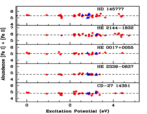
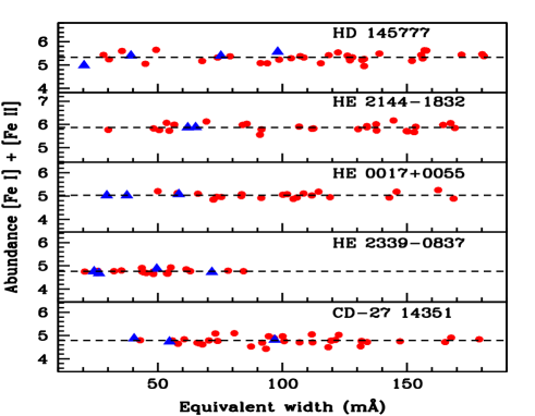
Figure 2: Iron abundances of stars for individual Fe I and Fe II lines as a function of excitation potential (top panel) and equivalent width (bottom panel). The solid red circles indicate Fe I lines and solid blue triangles indicate Fe II lines.

Table 4: Equivalent widths (in mÅ) of Fe lines used to derive atmospheric parameters.

Wavelength	Element	Elow	log gf	HD 145777	CD$-$27 14351	HE 0017$+$0055	HE 2144$-$1832	HE 2339$-$0837	References
(Å)		(eV)
4466.573	Fe I	0.11	$-$4.464	-	-	101.9 (5.08)	-	-	1
4476.019		2.85	$-$0.570	-	112.1 (4.71)	-	-	-	2
4871.318		2.87	$-$0.410	157.0 (5.63)	-	-	152.9 (5.67)	-	1

The numbers in parentheses in Cols. 5–9 give the derived abundances from the respective line.
References: 1. Fuhr et al. (1988), 2. Bridges & Kornblith (1974)
Note: This table is available in its entirety online. A portion is shown here for guidance regarding its form and content.

Table 5: Derived atmospheric parameters of our programme stars and literature values.

Star Name	Teff	log g	$\zeta$	[Fe I/H]	[Fe II/H]	[Fe/H]	Ref
	(K)	(cgs)	(km s-1)
HD 145777	4160	0.90	2.02	$-$2.17$\pm 0.18$	$-$2.17$\pm 0.25$	$-$2.17	1
	4245	-	-	-	-	-	2
	4216	-	-	-	-	-	7
CD$-$271 4351	4320	0.50	2.58	$-$2.72$\pm 0.16$	$-$2.69$\pm 0.07$	$-$2.71	1
	4335	0.50	2.42	-	-	$-$2.62	5
	4223	-	-	-	-	-	7
HE 0017$+$0055	4370	0.80	1.94	$-$2.47$\pm 0.12$	$-$2.45$\pm 0.03$	$-$2.46	1
	4250	1.00	2.00	-	-	$-$2.40	4
	4185	0.18	2.00	-	-	$-$2.72	6
HE 2144$-$1832	4190	0.60	1.87	$-$1.63$\pm 0.15$	$-$1.63$\pm 0.00$	$-$1.63	1
	4200	0.60	2.20	-	-	$-$1.70	3
HE 2339$-$0837	4940	1.40	1.55	$-$2.74$\pm 0.08$	$-$2.74$\pm 0.08$	$-$2.74	1
	4939	1.60	2.00	-	-	$-$2.71	6

References: 1. Our work, 2. Bergeat et al. (2001), 3. Hansen et al. (2016a), 4. Jorissen et al. (2016a), 5. Karinkuzhi et al. (2017), 6. Kennedy et al. (2011), 7. McDonald et al. (2012).

Table 6: Equivalent widths (in mÅ) of lines used to calculate elemental abundances.

Wavelength	Element	Elow	log gf	HD 145777	CD$-$27 14351	HE 0017$+$0055	HE 2144$-$1832	HE 2339$-$0837	References
(Å)		(eV)
5682.633	Na I	2.10	$-$0.700	40.2 (4.61)	52.9 (5.05)	-	69.8 (5.05)	36.3 (5.06)	1
5688.205		2.10	$-$0.450	45.1 (4.44)	51.0 (4.77)	-	93.7 (5.16)	47.2 (5.02)	1
6160.747		2.10	$-$1.260	-	-	-	45.1 (5.20)	-	1
4571.096	Mg I	0.00	$-$5.691	-	-	-	-	-	2
5528.405		4.35	$-$0.620	149.7 (6.42)	170.9 (6.70)	-	176.5 (6.71)	142.2 (7.03)	3

The numbers in parentheses in Cols. 5–9 give the derived abundances from the respective line.
References: 1. Kurucz & Peytremann (1975), 2. Laughlin & Victor (1974), 3. Lincke & Ziegenbein (1971)
Note: This table is available in its entirety online. A portion is shown here for guidance regarding its form and content.

6 Results

6.1 Abundance analysis

The abundances of various elements are determined from the measured equivalent widths of absorption lines due to neutral and ionised elements using the local thermodynamic equilibrium (LTE) analysis. Only the symmetric and clean lines are used for our analysis. As equivalent width measurement results depend on personal bias, to avoid it we also used the Tool for Automatic Measurement of Equivalent width (TAME) (Kang & Lee, 2012) to verify our measurements. TAME measures equivalent widths, determining the local continuum and using de-blending wherever necessary. A master line list (Table 6) is generated including all the elements, taking the excitation potential and log gf values from the Kurucz database of atomic line list and the measured equivalent widths. For our analysis we made use of the LTE line analysis and spectrum synthesis code MOOG 2013 (Sneden, 1973). The adopted model atmospheres are selected from the Kurucz grid of model atmospheres with no convective overshooting (http://kurucz.harvard.edu/grids.html). Elemental abundances of C, N, $\alpha$-elements, iron-peak elements, and several neutron-capture elements are estimated. We used spectrum synthesis calculations for the elements showing hyperfine splitting (e.g. Sc, V, Mn, Ba, La, and Eu). Several studies (Andrievsky et al., 2009, 2011; Hansen et al., 2013; Tremblay et al., 2013; Gallagher et al., 2016; Sitnova et al., 2016; Nordlander et al., 2017) in the past have focused on the 3D or NLTE or 3D-NLTE effects on the abundances of both heavy and light elements. However, we did not apply any NLTE corrections to our LTE estimates as the NLTE correction factors are negligible. The abundance results are presented in Tables 7 and 8. A comparison of our estimated abundance ratios with the literature values is presented in Table 9. We also estimated the carbon isotopic ratio ¹²C/¹³C and calculated [ls/Fe], [hs/Fe], and [hs/ls] for the stars, where ls represents Sr, Y, and Zr and hs represents Ba, La, Ce, and Nd. These results are presented in Table 10.

6.1.1 Carbon, nitrogen, oxygen

The abundance of oxygen could not be estimated as the oxygen lines are found to be blended and not usable for abundance estimates. The abundance of carbon is estimated using the spectrum synthesis calculation of the C₂ molecular bands near 5165 Å and 5635 Å, and the CH molecular band near 4310 Å. All three bands yield almost the same abundance of carbon for the respective stars (Tables 7 and 8). However, the CH molecular band in the spectrum of HE 2339$-$0837 could not be used as the band is saturated. Carbon is found to be enhanced ([C/Fe] $>$ 1) in all the stars. Our estimates of carbon abundance are higher than the carbon abundance reported for HE 2144$-$1832 in Hansen et al. (2016a). This discrepancy may be attributed to the lower resolution (R $\sim$ 7450) of the spectra used in Hansen et al. (2016a), whereas the resolution of our spectrum is R $\sim$ 60,000. One more reason for the discrepancy could be a difference in the adopted oxygen abundance. Estimates of carbon abundance depend on the adopted initial value of oxygen for the spectrum synthesis calculations. As the abundance of oxygen could not be estimated on our spectrum, we consider a solar value for oxygen (log$\epsilon$ = 8.69). The spectrum synthesis fits of C₂ and CH molecular bands for the stars are shown in Figures 3, 4, and 5.

The abundance of nitrogen is derived using the spectrum synthesis calculations of the only useful CN band at 4215 Å (Figure 6) using the estimated carbon abundance. Nitrogen is found to be enhanced in HE 0017$+$0055 and CD$-$27 14351 with [N/Fe] = 2.83 and 1.88, respectively. HD 145777 and HE 2144$-$1832 show moderate enhancement with [N/Fe] = 0.67 and 0.50, respectively. The CN band at 4215 Å is saturated in the spectrum of HE 2339$-$0837, and hence the abundance of N could not be estimated for this object.

We estimated the carbon isotopic ratio ¹²C/¹³C using the spectrum synthesis calculation of the ¹²CN and ¹³CN features near 8005 Å (Figure 7) and the ¹²C¹³C and ¹³C¹³C features near 4740 Å (Figure 8). The values of ¹²C/¹³C derived using these two features are presented in Table 10. We used the wavelengths, lower excitation potentials, and log gf values of different molecular transitions for the C₂ band at 5165 Å and CN bands from Brooke et al. (2013), Ram et al. (2014), and Sneden et al. (2014). The line lists of the C₂ bands at 5635 Å and 4740 Å, and the CH band at 4310 Å are taken from the linemake atomic and molecular line database.

Figure 3: Spectral synthesis plot of C₂ band around 5165 Å. The dotted lines indicate the synthesised spectra and the solid lines indicate the observed spectra. Two alternative synthetic spectra are shown corresponding to $\Delta$[C/Fe] = +0.01 (long-dashed line) and $\Delta$[C/Fe] = $-$0.01 (short-dashed line) in panel 1 (for HD 145777); $\Delta$[C/Fe] = +0.05 (long-dashed line) and $\Delta$[C/Fe] = $-$0.05 (short-dashed line) in panel 2 (for HE 2144$-$1832); $\Delta$[C/Fe] = +0.10 (long-dashed line) and $\Delta$[C/Fe] = $-$0.10 (short-dashed line) in panel 3 (for HE 0017+0055); $\Delta$[C/Fe] = +0.3 (long-dashed line) and $\Delta$[C/Fe] = $-$0.3 (short-dashed line) in panel 4 (for HE 2339$-$0837); and $\Delta$[C/Fe] = +0.01 (long-dashed line) and $\Delta$[C/Fe] = $-$0.01 (short-dashed line) in panel 5 (for CD$-$27 14351).

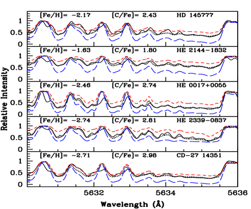
Figure 4: Spectral synthesis plot of C₂ band around 5635 Å. The dotted lines indicate the synthesised spectra and the solid lines indicate the observed spectra. Two alternative synthetic spectra are shown corresponding to $\Delta$[C/Fe] = +0.02 (long-dashed line) and $\Delta$[C/Fe] = $-$0.02 (short-dashed line) in panel 1 (for HD 145777); $\Delta$[C/Fe] = +0.15 (long-dashed line) and $\Delta$[C/Fe] = $-$0.15 (short-dashed line) in panel 2 (for HE 2144$-$1832); $\Delta$[C/Fe] = +0.05 (long-dashed line) and $\Delta$[C/Fe] = $-$0.05 (short-dashed line) in panel 3 (for HE 0017+0055); $\Delta$[C/Fe] = +0.3 (long-dashed line) and $\Delta$[C/Fe] = $-$0.3 (short-dashed line) in panel 4 (for HE 2339$-$0837); and $\Delta$[C/Fe] = +0.03 (long-dashed line) and $\Delta$[C/Fe] = $-$0.03 (short-dashed line) in panel 5 (for CD$-$27 14351).

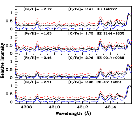
Figure 5: Spectral synthesis plot of CH band around 4310 Å. The dotted lines indicate the synthesised spectra and the solid lines indicate the observed spectra. Two alternative synthetic spectra are shown corresponding to $\Delta$[C/Fe] = +0.05 (long-dashed line) and $\Delta$[C/Fe] = $-$0.05 (short-dashed line) in panel 1 (for HD 145777); $\Delta$[C/Fe] = +0.15 (long-dashed line) and $\Delta$[C/Fe] = $-$0.15 (short-dashed line) in panel 2 (for HE 2144$-$1832); $\Delta$[C/Fe] = +0.30 (long-dashed line) and $\Delta$[C/Fe] = $-$0.30 (short-dashed line) in panel 3 (for HE 0017+0055); and $\Delta$[C/Fe] = +0.10 (long-dashed line) and $\Delta$[C/Fe] = $-$0.10 (short-dashed line) in panel 4 (for CD$-$27 14351).

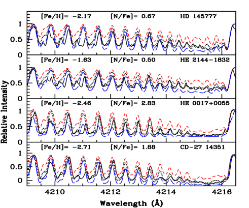
Figure 6: Synthesis of CN band around 4215 Å. The dotted line represents synthesised spectra and the solid line indicates the observed spectra. Two alternative fits, the short-dashed line corresponding to $\Delta$[N/Fe] = $-$0.3 and the long-dashed line corresponding to $\Delta$[N/Fe] = $+$0.3 are shown to illustrate the sensitivity of the line strengths to N abundance.

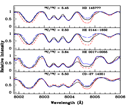
Figure 7: Spectral synthesis fits (dotted curves) of the CN features around 8005 Å obtained with the adopted C and N abundances and ¹²C/¹³C values (dotted curve). The observed spectrum is shown by a solid curve. Two alternative fits with ¹²C/¹³C $\sim$ 1 (short-dashed line) and 12 (long-dashed line) are shown to illustrate the sensitivity of the line strengths to the isotopic carbon abundance ratios.

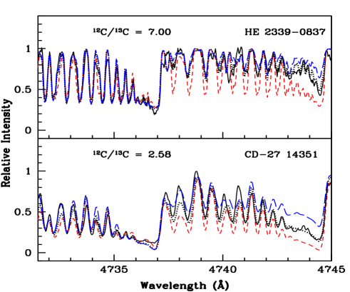
Figure 8: Spectral synthesis fits (dotted curves) of the C₂ features around 4740 Å obtained with the adopted C abundances and ¹²C/¹³C values (dotted curve). The observed spectrum is shown by a solid curve. Two alternative fits with ¹²C/¹³C $\sim$ 1 (short-dashed line) and 15 (long-dashed line) are shown to illustrate the sensitivity of the line strengths to the isotopic carbon abundance ratios.

6.1.2 Na, Mg, Ca, Sc, Ti, V

While HD 145777 and HE 2144$-$1832 show moderate enhancement in Na with [Na/Fe] = 0.45 and 0.53, respectively, HE 2339$-$0837 and CD$-$27 14351 exhibit enhanced abundance of Na with [Na/Fe] $>$ 1. Na abundance could not be estimated for HE 0017$+$0055 as the Na lines are severely blended and not usable for abundance estimates.

Magnesium and calcium are also found to be moderately enhanced in the stars HD 145777 and HE 2144$-$1832. While HE 2339$-$0837 and CD$-$27 14351 show enhanced abundance of Mg with [Mg/Fe] $>$ 1, Ca is found to be moderately enhanced with [Ca/Fe] in the range 0.4 to 0.9. We could not determine the abundance of Mg and Ca for HE 0017$+$0055 as no good lines were found.

We could estimate Sc abundance only for HD 145777 using spectrum synthesis calculations of the line Sc II 6245.637 Å considering the hyperfine splitting contributions from Prochaska & McWilliam (2000). This object shows mild enhancement of Sc with [Sc/Fe] = 0.77.

Titanium is estimated using lines from both neutral and ionised species for all the programme stars except HE 2339$-$0837, where Ti abundance is estimated only using Ti II lines. While Ti is found to be mildly enhanced in HD 145777, HE 2144$-$1832, HE 0017$+$0055, and HE 2339$-$0837, the object CD$-$27 14351 shows an overabundance with [Ti/Fe] $\sim$ 0.96. Although it is seen that due to NLTE effects, the abundances derived from Ti I and Ti II lines may differ (Johnson, 2002), we have derived similar abundances from Ti I and Ti II lines for our programme stars. The equal abundances found from Ti I and Ti II lines ensure the log g values estimated for our programme stars.

The abundances of V are found to be near solar with [V/Fe] $\sim$ $-$0.11 and 0.06 for HD 145777 and HE 2144$-$1832, respectively. V is highly abundant in CD$-$27 14351 with [V/Fe] = 1.11. For HE 0017+0055 and HE 2339$-$0837 abundance of V could not be estimated.

6.1.3 Cr, Mn, Co, Ni, Zn

The abundance of Cr is derived using seven Cr I lines (Table 6). Cr is underabundant with [Cr/Fe] = $-$0.21, $-$0.12, $-$0.50, and $-$0.34 for HD 145777, HE 2144$-$1832, HE 0017$+$0055, and HE 2339$-$0837, respectively. CD$-$27 14351 shows near solar abundance of Cr.

The abundance of Mn is estimated using spectrum synthesis calculations of the Mn I lines at 4765.846 Å and 4766.418 Å for HE 2144$-$1832, and the Mn II 5432.543 Å line is used for HD 145777. Mn is found to be underabundant in the stars HD 145777 and HE 2144$-$1832. The abundance of Mn could not be estimated for the other three objects as no suitable lines were detected for abundance determination.

The abundance of Co could be derived only for HD 145777 and HE 2144$-$1832, for which we obtained near solar values with [Co/Fe] = 0.03 and 0.06, respectively. The abundance of Co could not be estimated for the other three objects as no good lines were found for abundance estimation.

The abundance of Ni could be estimated only for HE 2144$-$1832 using equivalent width measurement of five Ni I lines (Table 6). Ni shows moderate enhancement in the star with [Ni/Fe] = 0.41. The abundance of Ni could not be estimated for the other objects as no good lines were found.

The abundance of Zn determined using Zn I 4810.528 Å line gives [Zn/Fe] = 0.63, $-$0.08, and 0.52 for the stars HD 145777, HE 2144$-$1832, and HE 0017$+$0055, respectively. The abundance of Zn could not be estimated for the other two objects as no suitable lines were detected for abundance determination.

6.1.4 Sr, Y, Zr

The abundance of Sr is estimated using spectrum synthesis calculations of the Sr I 4607.327 Å line for all the stars except HE 0017+0055 as this line is severely blended. While HD 145777 and HE 2144$-$1832 show moderate enhancement of Sr, it is found to be overabundant with [Sr/Fe] = 1.32 and 1.74 in HE 2339$-$0837 and CD$-$27 14351, respectively. The estimated Sr abundance is found to be $\sim$ 0.8 dex lower than that obtained by Hansen et al. (2016a) for the star HE 2144$-$1832 (Table 9), which they had obtained using the Sr II 4077.709 Å line on a spectrum of spectral resolution R ${\sim}$ 7450, and S/N = 6 (at 4000 Å). This line is severely blended in our spectrum, which was obtained at a higher resolution (R ${\sim}$ 60,000), and it could not be used for abundance analysis. The abundance estimated from the blended Sr II line in Hansen et al. (2016a) may be the reason for the observed discrepancy.

We estimated the abundance of Y using six lines (Table 6). HE 0017$+$0055 and HE 2339$-$0837 show mild overabundance with [Y/Fe] ${\sim}$ 0.58 and 0.67, respectively. The other three objects show overabundance of Y with [Y/Fe] $>$ 1.

Four Zr I lines and four Zr II lines (Table 6) are used to derive Zr abundance in the objects. Based on the availability, Zr I lines are used for HD 145777 and HE 2144$-$1832, and Zr II lines are used for HE 0017+0055 and HE 2339$-$0837. For the object CD$-$27 14351, both Zr I and Zr II lines could be used. Zr is found to be enhanced in all five stars.

We could not detect lines due to niobium (Nb) and technetium (Tc) in any of the spectra.

6.1.5 Ba, La, Ce, Pr, Nd

The abundance of Ba is derived using spectrum synthesis calculations of Ba II 5853.668 Å line for all five stars. Spectrum synthesis calculation of Ba II 6141.713 Å is also used to find the Ba abundance for HD 145777, HE 2339$-$0837, and CD$-$27 14351 (Figure 9). Both the lines gave similar abundance for the stars with the highest standard deviation of 0.15 for HE 2339$-$0837. The Ba II 6141.713 Å line could not be used to determine the abundance of Ba for the other two stars as the line is heavily blended in these two stars. The other two frequently used lines Ba II 4554.029 Å and Ba II 4934.076 Å are found to be severely blended in the spectra of the programme stars, and hence could not be used for abundance analysis. Hyperfine splitting contributions of the two lines used in the analysis are taken from McWilliam (1998). Ba is enhanced in all the stars with 1.27 $\leq$ [Ba/Fe] $\leq$ 2.30.

The abundance of La is estimated using the spectrum synthesis calculation of La II 4921.776 Å and found to be overabundant in all five stars with 1.37 $\leq$ [La/Fe] $\leq$ 2.46. La II 4808.996 Å line is also used for HE 0017$+$0055. Hyperfine splitting contributions of La II 4921.776 Å line are taken from Jonsell et al. (2006).

The abundance of Ce, Pr, and Nd are estimated using the equivalent width measurement technique. Twelve Ce II lines, 3 Pr II lines, and 13 Nd II lines (Table 6) are examined to derive the abundance of Ce, Pr, and Nd. Ce is found to be overabundant in all five stars. For the object CD$-$27 14351 we find a much lower value ([Ce/Fe] = 1.89) than the $\sim$ 2.63 found by Karinkuzhi et al. (2017). Karinkuzhi et al. (2017) used two lines Ce II 4460.207 Å and 4527.348 Å for Ce abundance estimate. We used three lines Ce II 4460.207 Å, 4483.893 Å, and 5187.458 Å. For the line Ce II 4460.207 Å, which is common in both the studies, our measured equivalent width is $\sim$ 160 mÅ, about 14 mÅ higher than in Karinkuzhi et al. (2017). This line, however, returned an abundance value that is $\sim$ 0.7 dex lower. In order to check whether the difference in abundance is due to the adopted model atmosphere, we calculated the abundance of Ce using the measured equivalent width ($\sim$ 146 mÅ) of this line by Karinkuzhi et al. (2017) and also the model atmosphere adopted by them. The derived abundance is found to be [Ce/Fe] = 1.72, which is closer to our estimated value. The other line, Ce II 4527.348 Å, used in their study is found to be severely blended in our spectrum.

Praseodymium (Pr) is found to be overabundant in all the stars with 1.67 $\leq$ [Pr/Fe] $\leq$ 2.42. Neodymium (Nd) is also found to be enhanced in all the stars with 1.37 $\leq$ [Nd/Fe] $\leq$ 2.55.

6.1.6 Sm, Eu

The abundance of Sm is derived using six Sm II lines (Table 6). No Sm lines could be found for CD$-$27 14351, hence Sm abundance could not be estimated for this object. The other four objects show enhanced abundance of Sm.

The abundance of Eu is derived using the spectrum synthesis calculation of the Eu II 6645.064 Å line (Figure 10) considering hyperfine splitting contributions from Worley et al. (2013). The other frequently used lines, Eu II 4129.725 Å, 4205.042 Å, and 6437.640 Å, are severely blended, and hence could not be used for abundance analysis. Eu shows overabundance with 0.80 $\leq$ [Eu/Fe] $\leq$ 2.14, except in CD$-$27 14351, for which we could estimate an upper limit with [Eu/Fe] ${\sim}$ 0.39. As shown in Figure 10, the Eu II 6645.064 Å line is blended with two CN lines. It can be clearly seen that the Eu II 6645.064 Å line is absent in the spectrum of the object CD$-$27 14351; a misidentification of the CN line at 6644.750 Å as the Eu II 6645.064 Å line could result in a much higher abundance of Eu; this may explain the very high abundance recorded for Eu by Karinkuzhi et al. (2017).

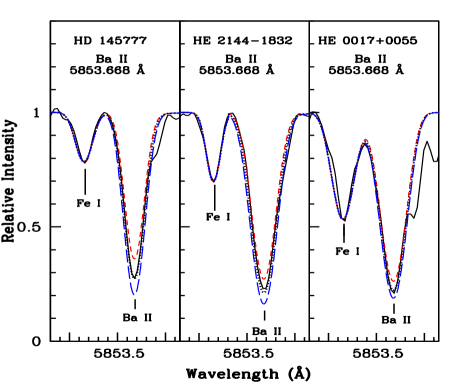
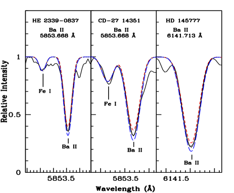
Figure 9: Spectral synthesis of Ba II 5853 Å and 6141 Å lines. Dotted line represents synthesised spectra and the solid line indicates the observed spectra. Two alternative fits, short dashed line corresponding to $\Delta$[Ba II/Fe] = $-$0.3 and long dashed line corresponding to $\Delta$[Ba II/Fe] = $+$0.3 are shown to illustrate the sensitivity of line strength to Ba abundance.

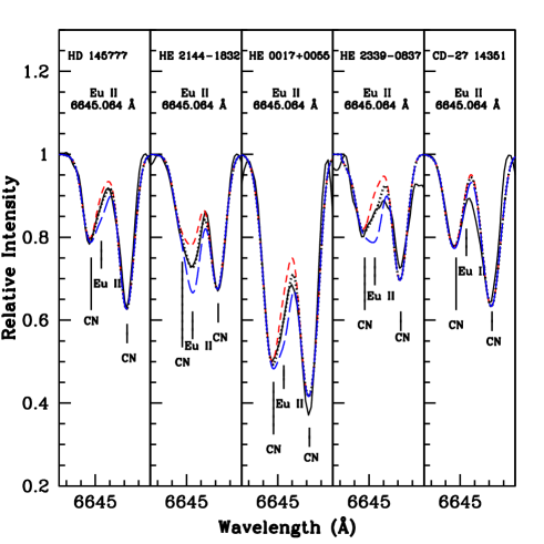
Figure 10: Synthesis of Eu II 6645 Å line. Dotted line represents synthesised spectra and the solid line indicates the observed spectra. Two alternative fits, short dashed line corresponding to $\Delta$[Eu II/Fe] = $-$0.3 and long dashed line corresponding to $\Delta$[Eu II/Fe] = $+$0.3 are shown to illustrate the sensitivity of line strength to Eu abundance.

Table 7: Elemental abundances in HD 145777, CD$-$27 14351, and HE 0017$+$0055

	HD 145777						CD$-$27 14351		HE 0017$+$0055
Element	Z	solar $log{\epsilon}^{a}$	$log{\epsilon}$	[X/H]	[X/Fe]	$log{\epsilon}$	[X/H]	[X/Fe]	$log{\epsilon}$	[X/H]	[X/Fe]
			(dex)			(dex)			(dex)
C (C2, 5165 Å)	6	8.43	8.69 (syn)	0.26	2.43	8.70 (syn)	0.27	2.98	8.70 (syn)	0.27	2.73
C (C2, 5635 Å)	6	8.43	8.69 (syn)	0.26	2.43	8.70 (syn)	0.27	2.98	8.71 (syn)	0.28	2.74
C (CH, 4310 Å)	6	8.43	8.67 (syn)	0.24	2.41	8.70 (syn)	0.27	2.98	8.73 (syn)	0.30	2.76
N (CN, 4215 Å)	7	7.83	6.33 (syn)	$-$1.50	0.67	7.00 (syn)	$-$0.83	1.88	8.20 (syn)	0.37	2.83
Na i	11	6.24	4.52$\pm$0.12 (2)	$-$1.72	0.45	4.91$\pm$0.20 (2)	$-$1.33	1.38	-	-	-
Mg i	12	7.60	6.25$\pm$0.23 (2)	$-$1.35	0.82	6.70 (1)	$-$0.90	1.81	-	-	-
Ca i	20	6.34	4.66$\pm$0.21 (9)	$-$1.68	0.49	4.54$\pm$0.20 (5)	$-$1.80	0.91	-	-	-
Sc ii	21	3.15	1.75 (syn)	$-$1.40	0.77	-	-	-	-	-	-
Ti i	22	4.95	3.44$\pm$0.17 (2)	$-$1.51	0.66	3.19$\pm$0.20 (3)	$-$1.76	0.95	3.13 (1)	$-$1.82	0.64
Ti ii	22	4.95	3.43$\pm$0.08 (5)	$-$1.52	0.65	3.20$\pm$0.13 (5)	$-$1.75	0.96	3.14$\pm$0.05 (3)	$-$1.81	0.65
V i	23	3.93	1.65 (syn)	$-$2.28	$-$0.11	2.33 (syn)	$-$1.60	1.11	-	-	-
Cr i	24	5.64	3.26$\pm$0.13 (6)	$-$2.38	$-$0.21	3.11$\pm$0.18 (3)	$-$2.53	0.18	2.68 (1)	$-$2.96	$-$0.50
Mn i	25	5.43	-	-	-	-	-	-	-	-	-
Mn ii	25	5.43	2.45 (syn)	$-$2.98	$-$0.81	-	-	-	-	-	-
Fe i	26	7.50	5.33$\pm$0.18 (33)	$-$2.17	-	4.78$\pm$0.16 (33)	$-$2.72	-	5.03$\pm$0.12 (21)	$-$2.47	-
Fe ii	26	7.50	5.33$\pm$0.25 (4)	$-$2.17	-	4.81$\pm$0.07 (3)	$-$2.69	-	5.05$\pm$0.03 (3)	$-$2.45	-
Co i	27	4.99	2.85 (1)	$-$2.14	0.03	-	-	-	-	-	-
Ni i	28	6.22	-	-	-	-	-	-	-	-	-
Zn i	30	4.56	3.02 (1)	$-$1.54	0.63	-	-	-	2.62 (1)	$-$1.94	0.52
Sr i	38	2.87	1.37 (syn)	$-$1.50	0.67	1.90 (syn)	$-$0.97	1.74	-	-	-
Y ii	39	2.21	1.26$\pm$0.02 (2)	$-$0.95	1.22	1.47$\pm$0.10 (3)	$-$0.74	1.97	0.33$\pm$0.08 (3)	$-$1.88	0.58
Zr i	40	2.58	1.46$\pm$0.14 (2)	$-$1.12	1.05	2.07 (1)	$-$0.51	2.20	-	-	-
Zr ii	40	2.58	-	-	-	2.09 (1)	$-$0.49	2.22	1.67$\pm$0.20 (3)	$-$0.91	1.55
Ba ii	56	2.18	1.28 (syn)$\pm$0.03	$-$0.90	1.27	1.29 (syn)$\pm$0.09	$-$0.89	1.82	2.02 (syn)	$-$0.16	2.30
La ii	57	1.10	0.30 (syn)	$-$0.80	1.37	$-$0.05 (syn)	$-$1.15	1.56	1.10 (syn)$\pm$0.20	0.0	2.46
Ce ii	58	1.58	1.20$\pm$0.09 (5)	$-$0.38	1.79	0.76$\pm$0.16 (3)	$-$0.82	1.89	1.23$\pm$0.06 (2)	$-$0.35	2.11
Pr ii	59	0.72	0.22$\pm$0.00 (2)	$-$0.50	1.67	$-$0.03 (1)	$-$0.75	1.96	0.68 (1)	$-$0.04	2.42
Nd ii	60	1.42	0.73$\pm$0.18 (5)	$-$0.69	1.48	0.08$\pm$0.16 (6)	$-$1.34	1.37	1.21$\pm$0.11 (4)	$-$0.21	2.25
Sm ii	62	0.96	0.42$\pm$0.03 (2)	$-$0.54	1.63	-	-	-	0.48$\pm$0.04 (2)	$-$0.48	1.98
Eu ii	63	0.52	$-$0.85 (syn)	$-$1.37	0.80	$<-$1.80 (syn)	$<-$2.32	$<$ 0.39	0.20 (syn)	$-$0.32	2.14

^a Asplund et al. (2009). The numbers in parentheses in Cols. 4, 7, and 10 show the number of lines used for the abundance determination.

Table 8: Elemental abundances in HE 2144$-$1832 and HE 2339$-$0837

	HE 2144$-$1832						HE 2339$-$0837
Element	Z	solar $log{\epsilon}^{a}$	$log{\epsilon}$	[X/H]	[X/Fe]	$log{\epsilon}$	[X/H]	[X/Fe]
			(dex)			(dex)
C (C2, 5165 Å)	6	8.43	8.65 (syn)	0.22	1.85	8.73 (syn)	0.30	3.04
C (C2, 5635 Å)	6	8.43	8.60 (syn)	0.17	1.80	8.50 (syn)	0.07	2.81
C (CH, 4310 Å)	6	8.43	8.55 (syn)	0.12	1.75	-	-	-
N (CN, 4215 Å)	7	7.83	6.70 (syn)	$-$1.13	0.50	-	-	-
Na i	11	6.24	5.14$\pm$0.08 (3)	$-$1.10	0.53	5.04$\pm$0.03 (2)	$-$1.20	1.54
Mg i	12	7.60	6.64$\pm$0.11 (2)	$-$0.96	0.67	7.03 (1)	$-$0.57	2.17
Ca i	20	6.34	5.11$\pm$0.17 (8)	$-$1.23	0.40	4.09$\pm$0.14 (4)	$-$2.25	0.49
Ti i	22	4.95	3.53$\pm$0.13 (6)	$-$1.42	0.21	-	-	-
Ti ii	22	4.95	3.51$\pm$0.05 (3)	$-$1.44	0.19	2.62$\pm$0.15 (4)	$-$2.33	0.41
V i	23	3.93	2.36 (syn)	$-$1.57	0.06	-	-	-
Cr i	24	5.64	3.89$\pm$0.18 (4)	$-$1.75	$-$0.12	2.56 (1)	$-$3.08	$-$0.34
Mn i	25	5.43	3.20 (syn)$\pm$0.0	$-$2.23	$-$0.60	-	-	-
Fe i	26	7.50	5.87$\pm$0.15 (27)	$-$1.63	-	4.76$\pm$0.08 (19)	$-$2.74	-
Fe ii	26	7.50	5.87$\pm$0.00 (2)	$-$1.63	-	4.76$\pm$0.08 (4)	$-$2.74	-
Co i	27	4.99	3.42$\pm$0.03 (3)	$-$1.57	0.06	-	-	-
Ni i	28	6.22	5.00$\pm$0.16 (5)	$-$1.22	0.41	-	-	-
Zn i	30	4.56	2.85 (1)	$-$1.71	$-$0.08	-	-	-
Sr i	38	2.87	1.90 (syn)	$-$0.97	0.66	1.45 (syn)	$-$1.42	1.32
Y ii	39	2.21	1.74$\pm$0.08 (3)	$-$0.47	1.16	0.14$\pm$0.10 (3)	$-$2.07	0.67
Zr i	40	2.58	1.92$\pm$0.18 (3)	$-$0.66	0.97	-	-	-
Zr ii	40	2.58	-	-	-	1.48 (1)	$-$1.10	1.64
Ba ii	56	2.18	2.04 (syn)	$-$0.14	1.49	1.65 (syn)$\pm$0.15	$-$0.53	2.21
La ii	57	1.10	1.00 (syn)	$-$0.10	1.53	0.60 (syn)	$-$0.50	2.24
Ce ii	58	1.58	1.65$\pm$0.17 (6)	0.07	1.70	1.21$\pm$0.13 (3)	$-$0.37	2.37
Pr ii	59	0.72	0.81$\pm$0.17 (3)	0.09	1.72	0.24$\pm$0.22 (2)	$-$0.48	2.26
Nd ii	60	1.42	1.40$\pm$0.17 (7)	$-$0.02	1.61	1.23$\pm$0.10 (5)	$-$0.19	2.55
Sm ii	62	0.96	1.11$\pm$0.21 (3)	0.15	1.78	0.51$\pm$0.14 (3)	$-$0.45	2.29
Eu ii	63	0.52	$-$0.10 (syn)	$-$0.62	1.01	$-$0.38 (syn)	$-$0.90	1.84

^a Asplund et al. (2009). The numbers in parentheses in Cols. 4 and 7 show the number of lines used for the abundance determination.

Table 9: Comparison of the abundances of our programme stars with the literature values

Star Name	[Fe/H]	[C/Fe]∗	[N/Fe]	[Sr/Fe]	[Y/Fe]	[Zr/Fe]	[Ba II/Fe]	Ref
HD 145777	$-$2.17	2.42	0.67	0.67	1.22	1.05	1.27	1
CD$-$27 14351	$-$2.71	2.98	1.88	1.74	1.97	2.21	1.82	1
	$-$2.62	2.89	1.89	1.73	1.99	-	1.77	4
HE 0017$+$0055	$-$2.46	2.74	2.83	-	0.58	1.55	2.30	1
	$-$2.40	2.17	2.47	-	0.50	1.60	$>$ 1.90	3
	$-$2.72	2.31	0.52	-	-	-	-	5
HE 2144$-$1832	$-$1.63	1.80	0.50	0.66	1.16	0.97	1.49	1
	$-$1.70	0.80	0.60	1.50	-	-	1.30	2
HE 2339$-$0837	$-$2.74	2.93	-	1.32	0.67	1.64	2.21	1
	$-$2.71	2.71	-	-	-	-	-	5
Star Name	[La II/Fe]	[Ce II/Fe]	[Pr II/Fe]	[Nd II/Fe]	[Sm II/Fe]	[Eu II/Fe]		Ref
HD 145777	1.37	1.79	1.67	1.48	1.63	0.80		1
CD$-$27 14351	1.56	1.89	1.96	1.37	-	$<$ 0.39		1
	1.57	2.63	-	1.26	-	1.65		4
HE 0017$+$0055	2.46	2.11	2.42	2.25	1.98	2.14		1
	2.40	2.00	-	2.20	1.90	2.30		3
	-	-	-	-	-	-		5
HE 2144$-$1832	1.53	1.70	1.72	1.61	1.78	1.01		1
	-	-	-	-	-	-		2
HE 2339$-$0837	2.24	2.37	2.26	2.55	2.29	1.84		1
	-	-	-	-	-	-		5

* $-$ Abundance of carbon is the average abundance derived from different molecular bands.

References: 1. Our work, 2. Hansen et al. (2016a), 3. Jorissen et al. (2016a), 4. Karinkuzhi et al. (2017), 5. Kennedy et al. (2011).

Table 10: Observed abundance ratios

Star Name	[Fe/H]	[ls/Fe]	[hs/Fe]	[hs/ls]	12C/13C	12C/13C	[Ba/Eu]	Ref
					(From CN band at 8005 Å)	(From C2 band at 4740 Å)
HD 145777	$-$2.17	0.98	1.48	0.50	5.45	5.50	0.47	1
CD$-$27 14351	$-$2.71	1.97	1.66	$-$0.31	5.50	2.58	-	1
	$-$2.62	1.82	1.77	$-$0.05	10.1	-	0.14	4
HE 0017$+$0055	$-$2.46	1.07	2.28	1.21	3.64	4.00	0.16	1
	$-$2.40	1.05	2.20	1.15	-	4.00	-	3
	-	-	-	-	-	1.30	-	2
HE 2144$-$1832	$-$1.63	0.93	1.58	0.65	2.50	2.50	0.48	1
	-	-	-	-	-	2.10	-	2
HE 2339$-$0837	$-$2.74	1.21	2.34	1.13	-	7.00	0.37	1

References: 1. Our work, 2. Goswami (2005), 3. Jorissen et al. (2016a), 4. Karinkuzhi et al. (2017).

6.2 Abundance uncertainties

Two components contribute to the total uncertainties on elemental abundances: random error and systematic error. In order to derive the uncertainties on the elemental abundances, we followed the procedure mentioned in Shejeelammal et al. (2020). We estimated the total uncertainties on log$\epsilon$ using the equation

$$\begin{split}\sigma^{2}_{log\epsilon}=&\sigma^{2}_{ran}+\left(\dfrac{\delta log\epsilon}{\delta T}\right)^{2}\sigma^{2}_{T_{eff}}+\left(\dfrac{\delta log\epsilon}{\delta logg}\right)^{2}\sigma^{2}_{logg}\\ &+\left(\dfrac{\delta log\epsilon}{\delta\zeta}\right)^{2}\sigma^{2}_{\zeta}+\left(\dfrac{\delta log\epsilon}{\delta[Fe/H]}\right)^{2}\sigma^{2}_{[Fe/H]}\end{split},$$ (1)

where $\sigma_{ran}$ is the random error that arises due to the uncertainties on the factors like equivalent width measurement, oscillator strength, and line blending. We adopted $\sigma_{ran}$ = $\dfrac{\sigma_{s}}{\sqrt{N}}$, where $\sigma_{s}$ is the standard deviation of the abundance of a particular species estimated using N number of lines of that species.

The typical uncertainties on the stellar atmospheric parameters T_eff, logg, $\zeta$, and [Fe/H] are denoted $\sigma_{T_{eff}}$, $\sigma_{logg}$, $\sigma_{\zeta}$, and $\sigma_{[Fe/H]}$, respectively. We evaluated the partial derivatives appearing in Equation 1 for the star HE 2144$-$1832, varying the stellar parameters T_eff, logg, $\zeta,$ and [Fe/H] by $\pm$ 100 K, $\pm$ 0.2 dex, $\pm$ 0.2 km/s^-1, and $\pm$ 0.2 dex, respectively. Finally, the uncertainties on [X/Fe] are derived as

$$\sigma^{2}_{[X/Fe]}=\sigma^{2}_{X}+\sigma^{2}_{[Fe/H]}.$$ (2)

The resulting differential abundances and the derived uncertainties on [X/Fe] are presented in Table 12. WE note that the calculated uncertainties on [X/Fe] are overestimated because of the assumption of the uncorrelated nature of the uncertainties arising from the different stellar parameters in Equation 1.

7 Kinematic analysis

Along with the physical parameters and composition it is also important to know the group of Galactic populations to which the programme stars belong. To determine this we calculated the space velocity for the stars using the method of Johnson & Soderblom (1987). Using the method given by Bensby et al. (2003) and information such as parallax ($\pi$) and proper motion ($\mu_{\alpha},\mu_{\delta}$) from the Gaia and SIMBAD databases (Gaia Collaboration et al., 2018) and radial velocity (V_r) from our estimates, we calculated the components of space velocity with respect to Local Standard of Rest (LSR) using the relation

$$(U,V,W)_{LSR}=(U,V,W)+(U,V,W)_{\odot}\leavevmode\nobreak\ {km/s}.$$ (3)

Here U, V, and W are the velocity vectors pointing towards the Galactic centre, the direction of Galactic rotation, and the Galactic north pole, respectively. The solar U, V, W component velocities (11.1, 12.2, 7.3) km/s are taken from Schönrich et al. (2010). The total spatial velocity (V_spa) is given by

$$V_{spa}=\sqrt{U_{LSR}^{2}+V_{LSR}^{2}+W_{LSR}^{2}}.$$ (4)

The detailed description of the calculations can be found in Purandardas et al. (2019). The estimated components of spatial velocity and the total spatial velocity are presented in Table LABEL:tab:kinematicresults. Following the procedures of Reddy et al. (2006), Bensby et al. (2003, 2004), and Mishenina et al. (2004), we calculated the probability that the stars are member of the thin disc, the thick disc, or the halo population. The estimated metallicity and spatial velocities indicate that three stars are members of the thick disc population. The probability estimates for them being members of the thick disc population are 0.83, 0.84, and 0.65 for HD 145777, HE 2144$-$1832, and HE 0017$-$0055, respectively. The probability estimates are 0.9 and 1.0 that the objects HE 2339$-$0837 and CD$-$27 14351, respectively, are members of the halo population (Table LABEL:tab:kinematicresults).

Table 11: Spatial velocity and probability estimates

Star Name	$U_{LSR}(km/s)$	$V_{LSR}(km/s)$	$W_{LSR}(km/s)$	$V_{spa}$ (km/s)	$P_{thin}$	$P_{thick}$	$P_{halo}$
HD 145777	$-$4.51 $\pm 3.22$	$-$155.01 $\pm 17.49$	67.18 $\pm 5.62$	169.00 $\pm 13.86$	0	0.83	0.17
CD$-$27 14351	101.95 $\pm 4.04$	$-$213.31 $\pm 24.66$	$-$57.21 $\pm 4.17$	243.25 $\pm 20.88$	0	0.10	0.90
HE 0017$+$0055	16.21 $\pm 2.02$	$-$190.74 $\pm 29.87$	$-$10.33 $\pm 15.90$	191.71 $\pm 30.31$	0	0.65	0.35
HE 2144$-$1832	234.33 $\pm 16.01$	8.57 $\pm 6.32$	$-$9.90 $\pm 9.09$	234.69 $\pm 15.82$	0.01	0.84	0.15
HE 2339$-$0837	218.78 $\pm 34.88$	$-$126.66 $\pm 37.83$	$-$224.20$\pm 14.05$	337.90 $\pm 4.18$	0	0	1.0

8 Discussion

We begin with a brief discussion on the formation scenarios of CEMP-s and CEMP-r/s stars from the literature, in the context of the stars in this study.

8.1 Formation scenarios of CEMP-(s & r/s) stars and their likelihoods

As discussed in Section 1, the widely accepted scenario to explain the enhancement of heavy elements exhibited by CEMP-s stars is that these objects are in binary systems with a now invisible white dwarf companions (as shown in Figure 11(a)). The observed enhancement of heavy elements in CD$-$27 14351 may be attributed to a binary companion in such a binary system. Various proposed formation scenarios that attempt to explain the unusual elemental abundance pattern of the CEMP-r/s stars are available in the literature. Jonsell et al. (2006) discussed nine scenarios explaining their origin, and concluded that none of the explanations was satisfactory. Lugaro et al. (2009) also discussed a few formation scenarios of this class of stars. In search of the most plausible formation mechanism, Abate et al. (2016) calculated the frequency of CEMP-r/s stars among CEMP-s stars, considering different formation scenarios discussed by Jonsell et al. (2006) and Lugaro et al. (2009), and compared that with the frequency of an observed sample of CEMP-r/s stars taken from the literature. A pictoral representation of some of these scenarios relevant to the present study is presented in Figure 11.

(a) AGB mass-transfer

(b) Self-pollution of a star formed from r-rich ISM

(c) AGB-pollution of a star in binary system formed from r-rich ISM

(d) SN and AGB pollution of a star in triple system

(e) AGB and 1.5 SN pollution of a star in binary system

(f) AGB and AIC pollution of a star in binary system

Figure 11: Representation of different proposed formation scenarios of CEMP-s and CEMP-r/s stars. M₁, M₂, and M₃ represent the masses of the stars, where M₁ $>$ M₂ $>$ M₃. Here evolutions of single, binary, and triple star systems with different conditions are shown. The figures are discussed individually in Sect. 8.1.

(i) Radiative levitation
This scenario is based on the fact that due to the large photon absorption cross sections of partially ionised heavy elements, they can be pushed outwards by radiative pressure that causes the abundances of heavy elements in the atmospheres of hot stars (e.g. Przybylski’s star) to appear much higher than the solar abundances. The observed abundance peculiarities of CEMP-r/s stars could also be thought of as a consequence of radiative levitation. However, as discussed in Cohen et al. (2003), Jonsell et al. (2006), and Abate et al. (2016), this scenario is rejected as a formation mechanism of CEMP-r/s stars. Richard et al. (2002) and Matrozis & Stancliffe (2016) have found from their simulations that radiative levitation is most effective in stars on the main sequence, and especially when they approach the turn-off as they have very thin convective envelopes. CEMP (-s & -r/s) stars are generally observed to be subgiants or giants and the effect of radiative levitation is found to be negligible in giants and low-temperature objects. All four objects that we have found to be enhanced in both s- and r-process elements are low-temperature (4160$-$4940 K) objects with log g values in the range 0.6 to 1.40 cgs units. Radiative levitation thus cannot be a process responsible for the observed overabundance of heavy elements in these stars.

(ii) Self-pollution of a star formed from r-rich ISM
This scenario (Hill et al., 2000; Cohen et al., 2003; Jonsell et al., 2006) is shown in Figure 11(b). As discussed in Jonsell et al. (2006) and Abate et al. (2016), this hypothesis may be rejected as none of the CEMP-r/s stars observed to date have been found to be in the evolutionary stage of AGB phase. The stars we studied are giants, and the estimated low ¹²C/¹³C values and the absence of Tc lines imply the extrinsic nature of the overabundance of carbon and heavy elements. This scenario thus cannot explain the abundance pattern observed in our programme stars.

(iii) SN and AGB pollution of a star in triple system
Figure 11(d) shows this scenario (Cohen et al., 2003; Jonsell et al., 2006). Both Cohen et al. (2003) and Jonsell et al. (2006) dismissed this scenario because it seems very unrealistic that the triple system survives such a nearby SN explosion for further mass transfer. Abate et al. (2016) also rejected this hypothesis, failing to reproduce the observed frequency of CEMP-r/s stars.

(iv) AGB and 1.5 SN pollution of a star in a binary system
This scenario is shown in Figure 11(e) (Jonsell et al., 2006). It was shown by Zijlstra (2004) that at low metallicity, due to low mass-loss efficiency, the degenerate core of high-mass AGB star remains massive enough to reach the Chandrasekhar mass limit and explodes as a type 1.5 supernova (Iben & Renzini, 1983). However, type 1.5 supernova can disrupt the binary system by destroying the primary star (Nomoto et al., 1976; Iben & Renzini, 1983; Lau et al., 2008). As discussed in Abate et al. (2016), this hypothesis is also dismissed as most CEMP-r/s stars are found to be in binary systems (Lucatello et al., 2005).

(v) AGB and accretion-induced collapse (AIC) pollution of a star in a binary system
This scenario (Qian & Wasserburg, 2003; Cohen et al., 2003) is shown in Figure 11(f). The three phases of mass transfer seem problematic since the observed CEMP-r/s stars, in many cases, are found to be at the main-sequence turn-off making the accretion difficult (Lugaro et al., 2009). As discussed in Abate et al. (2016), a narrow orbital separation is required for this scenario, so that even after the first phase of mass transfer the stars stay close enough to fill the Roche-lobe for the next phase of mass transfer. However, taking this situation into account, the observed frequency of CEMP-r/s stars could not be reproduced (Abate et al., 2016). In addition, it is quite uncertain if this kind of collapse can produce r-process elements so as to match the observed abundance pattern of the CEMP-r/s stars (Qian & Woosley, 1996; Qian & Wasserburg, 2003).

(vi) Intermediate neutron-capture process (i-process)
In their simulations Cowan & Rose (1977) found that a significantly high neutron flux (higher than that of s-process) can be produced by mixing different amounts of hydrogen-rich material into the intershell region of AGB stars (also known as proton ingestion episodes or PIEs), leading to the occurrence of i-process nucleosynthesis in AGB stars. This nucleosynthesis process operating at a neutron density (n $\sim$ 10¹⁵ cm^-3), which is intermediate to that of s- and r-process neutron densities can produce both s- and r-process elements in a single stellar site (Dardelet et al., 2014; Hampel et al., 2016; Roederer et al., 2016; Hampel et al., 2019). Hampel et al. (2016) successfully reproduced the abundance distribution of 20 CEMP-r/s stars with the help of an i-process model. Although it is evident that the i-process can explain the abundance pattern seen in CEMP-r/s stars, the astrophysical sites of the i-process are not clearly understood. A variety of sites have been proposed where PIEs can take place, favouring the conditions for i-process nucleosynthesis.

Figure 11(a) shows the formation scenario of CEMP-r/s stars, which is similar to that suggested for CH, Ba, and CEMP-s stars. In this scenario these stars are secondary in binary systems, where the primary, which is slightly more massive, evolves to the AGB phase and transfers s-process rich elements to the secondary star. The only difference in the scenario for CEMP-r/s stars is that the primary produces both s- and r-process elements in the AGB phase with the help of i-process nucleosynthesis, and later pollutes the secondary with both s- and r-process elements. Recent simulations have shown that higher neutron densities of the order of 10^12-15 cm^-3 necessary for i-process are attained in very metal-poor AGB stars (Campbell & Lattanzio, 2008; Cristallo et al., 2009; Campbell et al., 2010; Stancliffe et al., 2011). The reactions ¹³C($\alpha$, n)¹⁶O and ²²Ne($\alpha$, n)²⁵Mg are the two neutron sources proposed to operate in AGB stars. The reaction ²²Ne($\alpha$, n)²⁵Mg that can produce a neutron density of $\sim$ 10^11-14 cm^-3 needs a temperature of $\sim$ 3$\times$10⁸ K for activation, which is achieved only in intermediate-mass stars (M $\geq$ 3 M$\odot$) at the thermal pulse (TP) phase (Lugaro et al., 2012). As this phase is very short (a few days), in spite of high neutron density, neutron exposure remains inefficient to produce the heavy-s process peak (Fishlock et al., 2014). Again, the ¹³C($\alpha$, n)¹⁶O neutron source gets activated at a lower temperature ($\sim$ 1$\times$10⁸ K), and hence can operate in the interpulse phase of both low- and intermediate-mass AGB stars. Although this reaction can produce a neutron density of $\sim$ 10⁷ cm^-3, the longer timescale ($\sim$10⁵ years) of the interpulse phase enables sufficient neutron exposure to produce the heavy-s peak. However, some authors (Masseron et al., 2010; Jorissen et al., 2016a) argue in favour of the ²²Ne($\alpha$, n)²⁵Mg reaction as the primary neutron source responsible for the production of the abundance peculiarity observed in CEMP-r/s stars. The isotopic ratio of Mg could provide sufficient clues about the neutron source. The operation of ²²Ne($\alpha$, n)²⁵Mg reaction produces a large amount of ²⁵Mg, which in turn produces ²⁶Mg by neutron-capture. So, we can expect the ²⁴Mg : ²⁵Mg : ²⁶Mg ratio to change from the terrestrial (79 : 10 : 11) value to a ratio with higher abundances of ²⁵Mg and ²⁶Mg (Scalo, 1978). However, Zamora et al. (2004) attempted to determine Mg isotopic ratios from MgH bands in cool carbon stars and concluded that at optical wavelengths it is not possible to derive the Mg isotopic ratios as the synthetic spectra are insensitive to variations of Mg isotopic ratios due to the presence of strong C₂ and CN molecular bands. Thus, the scope of finding a spectroscopic test to identify the neutron source responsible for the production of heavy elements in CEMP-r/s stars still remains open.

Another site proposed for the i-process nucleosynthesis, supporting binary mass-transfer scenario for the formation of CEMP-r/s stars, is the very late thermal pulse (VLTP) in post-AGB stars (Herwig et al., 2011). The abundance pattern of Sakurai’s object (V4334 Sagittarii), a born-again giant, could not be reproduced by s-process yields. This object shows an overabundance of Rb, Sr, and Y that is two orders of magnitude higher than that of the second s-process peak (Asplund et al., 1999). Assuming proton ingestion into the He-shell convection zone, Herwig et al. (2011) carried out a 3D hydrodynamic simulation of a VLTP in a pre-white dwarf. They achieved a significantly high neutron density ( 10¹⁵ cm^-3) and could successfully reproduce the abundance distribution of Sakurai’s object. The post-AGB stars in the Large and Small Magellanic Clouds (LMC and SMC, respectively) are found to exhibit an unusual abundance pattern (van Winckel, 2003). Lugaro et al. (2015) illustrated that the s-process cannot explain the abundance pattern of these stars and proposed that i-process might explain better the abundances of the heavy elements along with the measured low abundance of Pb. Later, Hampel et al. (2019) could satisfactorily fit the abundance patterns observed in seven Pb-poor post-AGB stars (including the post-AGB stars of LMC and SMC) with i-process models.

Simulations of super-AGB TP stars showed that proton ingestion into the convective He-burning shell is favoured following the production of i-process neutron density (Doherty et al., 2015; Jones et al., 2016). Metal-poor massive stars (20 $-$ 30 M_⊙) are also considered as i-process sites (Banerjee et al., 2018; Clarkson et al., 2018). A single CEMP-r/s star can form from the ISM contaminated by the i-process material ejected by metal-poor massive stars (Banerjee et al., 2018).

One more proposed site for i-process nucleosynthesis is rapidly accreting white dwarf (RAWDs) (Denissenkov et al., 2017; Côté et al., 2018; Denissenkov et al., 2019). Denissenkov et al. (2019) proposed that single CEMP-r/s stars could be the tertiary (with a wider orbit) in a triple star system, where it orbits a close binary with a RAWD. Later the tertiary escapes from the triple star system being polluted by i-process material from the RAWD when the RAWD explodes as a SNIa. Due to the requirement of a particular sequence of events, population synthesis calculations can only decide the probability of the formation of CEMP-r/s stars from RAWDs (Hampel et al., 2019).

Roederer et al. (2016) reported a metal-poor star HD 94028 with underabundance of carbon ([C/Fe] = -0.06), and low Ba and Eu abundances. With the help of high-quality NUV spectra, they could estimate the abundances or upper limits of 64 species of 56 elements including the species whose features are seen mostly in the NUV. Roederer et al. (2016) found that the star exhibits a supersolar [As/Ge] ratio, a solar [Se/As] ratio, and enhanced abundances of Mo and Ru. They could not reproduce this elemental pattern with any combination of s and r-process, but an additional contribution from the i-process could fit the peculiar pattern. The contribution of i-process has also been observed in pre-solar grains in pristine meteorites (Fujiya et al., 2013; Liu et al., 2014). These observations indicate more than one astrophysical sites for the i-process.

(vii) AGB pollution of a star in binary system formed from r-rich ISM
This scenario (Hill et al., 2000; Cohen et al., 2003; Jonsell et al., 2006; Ivans et al., 2005; Bisterzo et al., 2011) is illustrated in Figure 11(c). Although Bisterzo et al. (2011, 2012) claim to reproduce, within the error bars, the observed [hs/ls] (which is higher in CEMP-r/s stars than CEMP-s stars) considering the binary system formed from the r-rich molecular cloud, there are several arguments that stand against this scenario. It was noted that in the case of independent s- and r-process enrichment, the correlation of the abundances of Ba and Eu cannot be reproduced by the AGB models (Abate et al., 2016), and also that this scenario cannot explain the large fraction of CEMP-r/s stars among the CEMP-s stars (Jonsell et al., 2006; Lugaro et al., 2009).

As the abundance patterns of most of the CEMP-r/s stars found in the literature can be explained with i-process models, some authors prefer the nomenclature ‘CEMP-i’ to ‘CEMP-r/s’ (Hampel et al., 2016; Frebel, 2018; Hampel et al., 2019) and calling the stars formed by AGB pollution in the binary system formed from r-rich ISM ‘CEMP-r+s stars’ (Gull et al., 2018; Frebel, 2018).

Gull et al. (2018) reported a red giant CEMP star RAVE J094921.8$-$161722 ([Fe/H] = $-$2.2, [C/Fe] = 1.35) with a surprising elemental abundance pattern. The star exhibits an enhanced abundance of Pb, indicating s-process contribution and Th, which is produced in r-process nucleosynthesis. Gull et al. (2018) claimed that this object was the first bona fide CEMP-r+s star as its abundance pattern could be satisfactorily fitted only with AGB mass-transfer model taking into account initial r-process enhancement. Sbordone et al. (2020) reported the abundance analysis of object GIU J190734.24-315102.1 located in the Sagittarius (Sgr) dwarf spheroidal (dSph) galaxy, and claimed that the abundance pattern could be best fit only with a model considering AGB-pollution in a binary system pre-enriched with a neutron star–neutron star merger event. Sbordone et al. (2020) classify this object as the first CEMP-r/s star found in the Sgr dSph, but due to its formation scenario this object may be referred to as a bona fide CEMP-r+s star.

The expected rate of occurrence of CEMP-r+s stars among metal-poor stars is 2% $-$ 3% (Gull et al., 2018). With an occurrence rate of 3%, about two dozen r-II stars have been found to date (Gull et al., 2018), although why no other bona fide CEMP-r+s stars have yet been detected remains a puzzle (Frebel, 2018).

8.2 Comparison of the observed abundances of the programme stars with i-process model predictions

Hampel et al. (2016) calculated yields of heavy elements considering different constant neutron densities ranging from $10^{7}-10^{15}$ cm^-3 using single-zone nuclear network calculations. The nucleosynthesis is assumed to occur in the intershell region of AGB stars. The physical input parameters, such as temperature and density for the intershell region of a low-mass (1 M_⊙) low-metallicity (z = 10^-4) AGB star, are adapted from Stancliffe et al. (2011). The constituents of the intershell region have been adapted from that of Abate et al. (2015). The temperature and density of the intershell region are considered to be $1.5\times 10^{8}$ K and $\rho$ = 1600 gcm^-3, respectively. However, no significant changes in the results were found when tested with a range of temperatures ($1\times 10^{8}$ to $2.2\times 10^{8}$ K) and densities ($\rho$ = 800 gcm^-3 to 3200 gcm^-3). The run times of the models are adjusted in such a way that a high neutron exposure ($\tau$ $\sim$ 495 mb^-1) is ensured. Equilibrium abundance pattern between heavy elements and the seed nuclei is established based on such a high neutron exposure, and the element-to-element ratio becomes a function of constant neutron density. After the exposure the neutron flux is kept switched off for t = 10 Myr.

During the time when neutron flux is switched on, it should be noted that for lower neutron densities the elemental abundance pattern of typical s-process is produced with stable ls (Sr, Y, Zr) and hs (Ba, La, Ce) peaks. However, with i-process neutron densities (n = $10^{12}-10^{15}$ cm^-3), the neutron-capture path goes further away from the valley of stability, making both ls and hs peak shift to lighter elements; in particular, they form a peak at ¹³⁵I. Then, after the neutron exposure is switched off, it is found that the decay of unstable isotopes produce stable ls and hs peak elements, for example ¹³⁵I decays to produce ¹³⁵Ba. Abundances of Ba and Eu are found to increase with neutron density. This is how the i-process can modify the abundance pattern of neutron-capture elements.

We used the model yields ([X/Fe]) of Hampel et al. (2016), with neutron densities ranging from $10^{9}-10^{15}$ cm^-3, and compared them with the observed abundances of our programme stars. In order to find the neutron density responsible for the observed abundance distribution of the programme stars, we followed the procedure given in Hampel et al. (2016). We used the equation

$$X=X_{i}(1-d)+X_{\odot}d,$$ (5)

where $X_{i}$ is the model yield, $X_{\odot}$ is the solar-scaled abundance, and $d$ is a dilution factor.

Figure 12 shows the best-fit models with appropriate neutron densities and corresponding dilution factors. It is seen that the i-process model with neutron densities of n $\sim$ $10^{13}$ cm^-3, $10^{15}$ cm^-3, and $10^{14}$ cm^-3 closely fit the observed abundances of HE 2144$-$1832, HE 0017$+$0055, and HE 2339$-$0837, respectively. The best model fit for HD 145777 is found at a neutron density of n $\sim$ $10^{10}$ cm^-3.

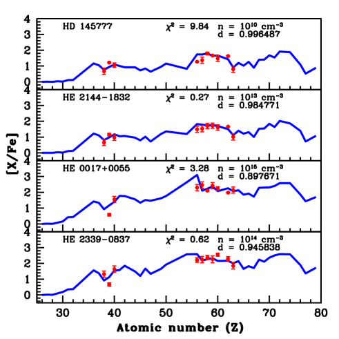
Figure 12: Best-fitting i-process model (solid blue curve) for the stars. The points with error bars indicate the observed abundances.

8.3 Classification of the programme stars

As discussed in Section 1, different authors (Beers & Christlieb, 2005; Jonsell et al., 2006; Masseron et al., 2010; Abate et al., 2016; Frebel, 2018; Hansen et al., 2019) have used different criteria to classify the CEMP stars into various subclasses. Four objects in our sample, HD 145777, HE 0017+0055, HE 2144$-$1832, and HE 2339$-$0837, show overabundances of Ba and Eu along with other light-s and heavy-s elements. With 0 $<$ [Ba/Eu] $<$ 0.5, all four objects fall in the category of CEMP-r/s stars if the classification criteria of Beers & Christlieb (2005) for CEMP-r/s stars is followed. But, according to the classification scheme of Abate et al. (2016), CEMP-r/s stars are those that have [Ba/Fe] and [Eu/Fe] values that are greater than unity. This criterion classifies HE 2144$-$1832 ([Ba/Fe] = 1.49 and [Eu/Fe] = 1.01), HE 0017$+$0055 ( [Ba/Fe] = 2.30 and [Eu/Fe] = 2.14), and HE 2339$-$0837 ([Ba/Fe] = 2.21 and [Eu/Fe] = 1.84) as CEMP-r/s stars, and HD 145777 (with [Ba/Fe] = 1.27 and [Eu/Fe] = 0.80) as a CEMP-s star. All four of these objects fall in the category of CEMP-r/s stars if we use the criteria 0.0 $<$ [La/Eu] $<$ 0.6 given by Frebel (2018) for the CEMP-i subclass (we use the ‘CEMP-r/s’ nomenclature). We could not estimate the abundances of Hf, Ir, and Pb, hence the other criteria, namely [Hf/Ir] $\sim$ 1.0 for the CEMP-i subclass and [Ba/Pb] $>$ $-$1.5 for the CEMP-s subclass put forward by Frebel (2018), could not be used. However, the lower limit given on [Ba/Eu] ($>$ 0.5) by Frebel (2018) for the CEMP-s subclass clearly indicates that these four stars cannot be classified as CEMP-s stars. If we use [Sr/Ba] as a classifier, as discussed in Hansen et al. (2019) with values [Sr/Ba] $\sim$ $-$0.60, $-$0.83, and $-$0.89 respectively for HD 145777, HE 2144$-$1832, and HE 2339$-$0837, they fall in the category of CEMP-r/s stars. As the abundance of Sr could not be estimated for the object HE 0017+0055, [Sr/Ba] could not be used to classify this object.

The object CD$-$27 14351 is found to satisfy the criteria for the CEMP-s stars of all four classification schemes, hence this object with [Ba/Fe] = 1.82, [Eu/Fe] $<$ 0.39, [Ba/Eu] $>$ 1.43, [La/Eu] $>$ 1.17, and [Sr/Ba] = $-$0.08 is classified as a CEMP-s star.

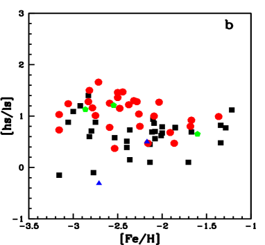
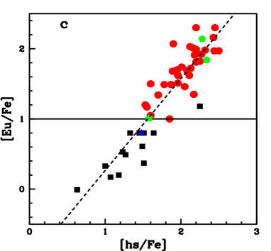
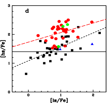
Figure 13: Probing [hs/ls] as a classifier of CEMP-s and CEMP-r/s stars. The filled red circles represent CEMP-r/s stars, filled black squares represent CEMP-s stars, and filled blue triangles and filled green pentagons respectively represent CEMP-s and CEMP-r/s stars in this work. In panel (a) $\mu$ and $\sigma$ represent the mean and standard deviation of [hs/ls] respectively for CEMP-s and CEMP-r/s stars. In panel (c) the short-dashed black line represents the correlation between [hs/Fe] and [Eu/Fe] for CEMP-s and CEMP-r/s stars. In panel (d) the short-dashed black line and long-dashed red line represent the correlation between [hs/Fe] and [ls/Fe] for CEMP-s and CEMP-r/s stars, respectively.

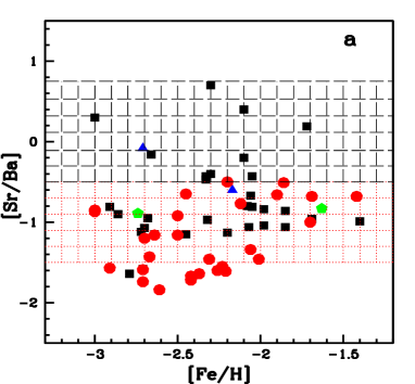
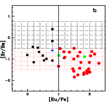
Figure 14: [Sr/Ba] as a classifier of CEMP-s and CEMP-r/s stars. The filled red circles represent CEMP-r/s stars, filled black squares represent CEMP-s stars, and filled blue triangles and filled green pentagons respectively represent CEMP-s and CEMP-r/s stars in this work. The grid formed by the dashed black lines represents the region of CEMP-s stars, and the grid formed by the dotted red lines represents the region of CEMP-r/s stars put forward by Hansen et al. (2019). In panel (b) the solid black line at [Eu/Fe] = 1.0 separates the CEMP-s and CEMP-r/s stars according to the classification criteria adopted by Abate et al. (2016).

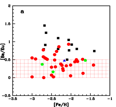
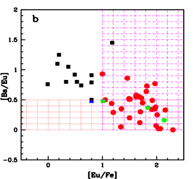
Figure 15: Same as Fig. 14, but for [Ba/Eu]. The filled red circles represent CEMP-r/s stars, filled black squares represent CEMP-s stars, and filled blue triangles and filled green pentagons respectively represent CEMP-s and CEMP-r/s stars in this work. The grid formed by the dotted red lines represents the region of CEMP-r/s stars put forward by Beers & Christlieb (2005). The grid formed by the dashed magenta lines represents the region of CEMP-r/s stars put forward by Abate et al. (2016).

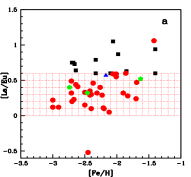
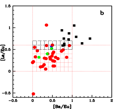
Figure 16: Same as Fig. 14, but for [La/Eu]. The filled red circles represent CEMP-r/s stars, filled black squares represent CEMP-s stars, and filled blue triangles and filled green pentagons respectively represent CEMP-s and CEMP-r/s stars in this work. In panel (a) the grid formed by the dotted red lines represents the region of CEMP-r/s stars put forward by Frebel (2018). In panel (b) we can see that all the CEMP-r/s stars but two fall inside the grid formed by the dotted red lines bound by 0.0 $<$ [La/Eu] $<$ 0.6 and 0.0 $<$ [Ba/Eu] $<$ 1.0. The grid formed by the black dashed lines bound by 0.5 $<$ [La/Eu] $<$ 0.7 represents the uncertain region in the upper boundary of the classification put forward by Frebel (2018) for CEMP-r/s stars.

8.3.1 Probing [hs/ls] as a classifier

It has been noted from various studies in the past (Bisterzo et al., 2011, 2012; Abate et al., 2015, 2016; Hampel et al., 2016) that [hs/ls] exhibit higher values for CEMP-r/s stars than that of CEMP-s stars. In this section we explore whether [hs/ls] can be used to distinguish CEMP-r/s and CEMP-s stars, and hence if this ratio can be used as a classifier.

To accomplish this we carried out a literature survey and compiled data for 40 CEMP-s and 32 CEMP-r/s stars, and calculated [hs/ls], [Sr/Ba], and [Ba/Eu] for these stars on a homogeneous scale. We adopt the CEMP classifications of the literature objects given by the original studies and without any ambiguity. However, for some objects different groups have provided different atmospheric parameters and elemental abundances, and have assigned different classes to them. For instance, Allen et al. (2012) considered HE 0336+0113 to be a CEMP-s star, but Masseron et al. (2010) considered it a CEMP-r/s star. HE 0336+0113 exhibits [Eu/Fe] $>$ 1.0 and shows the highest value of [Ba/Eu] (= 1.45) among the CEMP stars (Cohen et al., 2006). Hampel et al. (2019), after comparing the object’s observed abundances with i-process models, reported that the characteristic properties of HE 0336+0113 are more of s-process than i-process. This analysis prompted us to classify HE 0336+0113 as a CEMP-s star. Bisterzo et al. (2011, 2012) studied most of the CEMP-s stars in Table 13 and explained their abundance peculiarities with the help of AGB models with initial masses of 1.3 $-$ 2.0 M$\odot$. Except for SDSS J1349$-$0229, which is classified as a CEMP-r/s star (Behara et al., 2010), all other CEMP-r/s stars in Table 13 have been examined with i-process model predictions and their abundance patterns are well reproduced with i-process model yields (Hampel et al., 2016, 2019; Goswami & Goswami, 2020).

The elemental abundances of the objects reported by different authors differ from each other. As different authors use different codes, model atmospheres, and line lists for their abundance analyses, it is not surprising to see the differences in their results; however, it is not an easy task to select one analysis over the others. Thus, for the objects for which the elemental abundance results from several different groups are available, we take the mean value of [Fe/H], and similarly the mean abundance for each element. For these cases, we use the mean [X/Fe] to calculate [hs/ls], [Sr/Ba], and [Ba/Eu]. To calculate [ls/Fe], we take the mean of the abundances of light-s elements (Sr, Y, Zr); similarly, the abundances of heavy-s elements (Ba, La, Ce, Nd) are averaged out to calculate [hs/Fe]. We do not consider the two second peak s-process elements Pr and Sm, as r-process contributes more than s-process to the isotopic abundances of these elements (Arlandini et al., 1999). Bisterzo et al. (2012) noted that light-s elements when plotted against each other show large scatter. Heavy-s elements also show scatter for some objects, although not as large. In order to reduce the systematic error, we calculated [ls/Fe] and [hs/Fe] only for those stars for which abundance estimates are available at least for two light s-process and two heavy s-process elements. To calculate [ls/Fe] and [hs/Fe], we also excluded those elements for which only the upper limit of abundance is mentioned in the literature. Table 13 presents the list of objects and their elemental abundance ratios of C, N, and heavy elements used for this analysis. Our estimates of [hs/ls] are also presented in this table. Estimates of [hs/ls], when plotted with respect to [Fe/H], show a large scatter (Figure 13(b)). The use of different sets of elemental abundances instead of using a consistent set of elements for hs and ls abundances may also contribute to this observed scatter. Nevertheless, it is not always possible to have the same set of hs and ls elements for all stars, and using a consistent set of elements will tremendously affect the number of stars used to carry out the test. As metallicity decreases, the neutron-to-iron seed ratio increases and hence heavier elements are synthesised to a greater extent (i.e. [hs/ls] increases as metallicity decreases; Gallino et al. 1998). In Figure 13(b) we can clearly see this trend for both CEMP-s (black filled squares) and CEMP-r/s (red filled circles) stars. However, even though they have the same metallicity range, we note that the CEMP-r/s stars exhibit higher values of [hs/ls] than the CEMP-s stars (Bisterzo et al., 2011, 2012). This implies that neutron density has to be higher for the formation of CEMP-r/s stars than of CEMP-s stars. Similarly, in Figure 13(d), we can see that the mean abundances of ls elements have the same range in the cases of CEMP-s and CEMP-r/s stars, but in CEMP-r/s stars the hs elements are more enhanced than in CEMP-s stars. This indicates that the heavy elements observed in CEMP-r/s stars are synthesised with a higher neutron density than those in CEMP-s stars. This is because the higher neutron density can easily overcome the barrier ($\tau$ $\sim$ 0.05 mb^-1) at the magic neutron number 50 (the ls peak), and effectively produces the hs peak at the magic neutron number 82. As seen from Figure 13(c), [Eu/Fe] increases with [hs/Fe], showing a tight correlation between [Eu/Fe] and [hs/Fe]. This correlation between heavy-s elements and Eu observed in the CEMP-r/s stars can only be explained with the help of a formation mechanism where both the s-process and r-process elements are produced in a single stellar site, which provides much support for i-process as a possible formation mechanism for CEMP-r/s stars. As [hs/ls] does not depend upon the dilution of the AGB processed material on the companion star, using a sample of CEMP-s and CEMP-r/s stars from the literature, we examined whether this ratio could be used to distinguish between CEMP-s and CEMP-r/s stars. We find that CEMP-s stars peak at around [hs/ls]$\sim$0.65 with a standard deviation of 0.35, and CEMP-r/s stars peak at [hs/ls]$\sim$1.06 with a standard deviation of 0.32. However, even though they peak at different values of [hs/ls], we see an overlap of CEMP-s and CEMP-r/s stars in the range 0.0$<$[hs/ls]$<$1.5 (Figure 13(a) and 13(b)). Hence, [hs/ls] cannot be used as a useful classifier for CEMP-s and CEMP-r/s stars. In Figure 13(d) all the CEMP-r/s stars lie above the solid black line at [hs/Fe]$\sim$1.4; however, a limiting value of [hs/Fe]$\geq$1.4 also cannot be used as a classifier as many CEMP-s stars also exhibit [hs/Fe] $\geq$1.4.

8.3.2 Identification of classifier based on available data

In order to explain the nature of the emerging CEMP stars, Beers & Christlieb (2005) introduced for the first time four subclasses of CEMP stars using only two neutron-capture elements, Ba and Eu (due to the observational limitations). This scheme of classification is a guide to the community to use the unifying nomenclature and to facilitate further advances. However, since the classification of Beers & Christlieb (2005), various authors (Jonsell et al., 2006; Masseron et al., 2010; Norris et al., 2010; Bisterzo et al., 2011; Bonifacio et al., 2015; Maeder & Meynet, 2015; Yoon et al., 2016; Abate et al., 2016; Hansen et al., 2016c; Frebel, 2018; Hansen et al., 2019; Skúladóttir et al., 2020) put forward different criteria for identification and classification of the CEMP stars. The community has not had much time to understand the physics behind the observed abundance patterns. The ever-growing data sets and the advancement of theoretical predictions require further revisions of the classification schemes, and thus revisiting these classification schemes is extremely important and unavoidable.

We have seen that one of our programme stars, HD 145777, is classified as a CEMP-r/s star by three classification schemes (Beers & Christlieb, 2005; Frebel, 2018; Hansen et al., 2019) and as a CEMP-s star by the criteria discussed by Abate et al. (2016). So, we tried to figure out which of the classification scheme discussed above fits the literature data. As the programme stars are CEMP-s and CEMP-r/s types, we focus on the classification schemes that discuss the criteria to distinguish these two subclasses.

[Sr/Ba] as a classifier
We first discuss the most recent classifier, [Sr/Ba]. When we plot [Sr/Ba] versus [Fe/H] (Figure 14(a)), we can see that there is a clear overlap of CEMP-s and CEMP-r/s stars with respect to [Sr/Ba] (as seen in the case of [hs/ls]) in the range $-$1.6 $<$ [Sr/Ba] $<$ $-$0.5. In Figure 14(a)  and 14(b) the grid formed by the dashed black lines and the grid formed by the dotted red lines represent the region of CEMP-s and CEMP-r/s stars, respectively, put forward by the classification scheme of Hansen et al. (2019). In Figure 14(b), it is seen that a few CEMP stars (Table 13) with an underabundance of Eu ([Eu/Fe] $<$ 1.0) also fall in the region defined for CEMP-r/s stars. The number difference of CEMP-s stars in Figure 14(a) and 14(b) falling in the CEMP-r/s region indicates that many CEMP stars with the absence of Eu also fall in the category of CEMP-r/s stars by this classification criterion. We cannot separate CEMP-s and CEMP-r/s stars with the help of the [Sr/Ba] criterion (Hansen et al., 2019), and hence it cannot be used effectively. Moreover, it is worth mentioning that the abundances of Sr and Ba are highly uncertain due to NLTE effects (Bisterzo et al., 2012). However, as mentioned by Hansen et al. (2019), this criterion may be useful to roughly distinguish between the different CEMP subclasses in low-resolution, low S/N large surveys as absorption lines of Eu are much weaker than Sr.

[Ba/Eu] as a classifier
In Figure 15(a) and 15(b) the grid formed by the dotted red lines bound the region (0.0 $<$ [Ba/Eu] $<$ 0.5) allowed by Beers & Christlieb (2005) for CEMP-r/s stars. Although most of the CEMP-r/s stars (filled red circles), including our programme stars (filled green pentagons), reside inside the region, some fall outside the boundary. Abate et al. (2016) did not put an upper limit to [Ba/Eu] for CEMP-s and CEMP-r/s stars, so this criterion could be used more effectively (HE 0336+0113 is the only outlier). According to this criterion, CEMP-r/s stars are a subclass of CEMP-s stars and the criterion [Eu/Fe] $>$ 1.0 separates the CEMP-r/s stars from the CEMP-s stars (Abate et al., 2016). Jonsell et al. (2006) and Masseron et al. (2010) also adopted the same classification scheme as Abate et al. (2016) to distinguish between CEMP-s and CEMP-r/s stars; however, their criteria to classify the other two subclasses (CEMP-r & CEMP-no) differ. Abundances of many of the CEMP-r/s stars, (e.g. CS 22881$-$036, CS 29497$-$030, HE 0143$-$0441, HE 2258$-$6358, and LP 625$-$44) having [Ba/Eu] $>$ 0.5 are found to fit well with the i-process model (Hampel et al., 2016) of higher neutron density (n$\sim$10¹⁴ cm^-3) (Hampel et al., 2019). This is in contrast to 0.0 $<$ [Ba/Eu] $<$ 0.5 of Beers & Christlieb (2005) for CEMP-r/s stars and also [Ba/Eu] $>$ 0.5 of Frebel (2018) for CEMP-s stars.

[La/Eu] as a classifier
Unlike other classification schemes, Frebel (2018) used different sets of elements to classify CEMP-s and CEMP-r/s stars. While Ba, Eu, and Pb are used in the case of CEMP-s stars, La, Eu, Hf, and Ir are used to classify CEMP-r/s stars. The abundances of Hf and Ir are usually derived from the absorption lines of Hf and Ir that are normally found in the NUV spectra. As we could not get the abundances for these two elements in the literature, the criterion [Hf/Ir] $\sim$ 1.0 could not be tested with our compiled data. Theoretical validation of this criterion can be found in Table 4 of Hampel et al. (2016). In Figure 16(a), two CEMP-r/s stars are found to lie outside the region (the grid formed by dotted red lines) defined by 0.0 $<$ [La/Eu] $<$ 0.6, and two CEMP-s stars are located near the upper boundary ([La/Eu] $\sim$ 0.6) of the region.

Modifications to the classifiers [Ba/Eu] and [La/Eu]
Frebel (2018) kept provisions for future adjustments to the classifying criteria. In Figure 16(b), except for two stars (CD$-$28 1082 and HD 209621), all the CEMP-r/s stars fall inside the region (the grid formed by the dotted red lines) bound by 0.0 $<$ [La/Eu] $<$ 0.6 and 0.0 $<$ [Ba/Eu] $<$ 1.0. As a few CEMP-(s & r/s) stars also fall very close to the upper boundary, we can put uncertainty on the upper limit of [La/Eu] (i.e. [La/Eu] $<$ 0.6 $\pm$ 0.1). We suggest that an object satisfying the criteria 0.0 $<$ [Ba/Eu] $<$ 1.0 and 0.0 $<$ [La/Eu] $<$ 0.5 can be classified as a CEMP-r/s star; however, if [La/Eu] = 0.6 $\pm$ 0.1 the condition [Eu/Fe] $>$ 1.0 also needs to be satisfied for the star to be a CEMP-r/s star. The two outliers exhibit differences in the range 0.5$-$0.7 dex between the abundances of La and the other hs elements. In Figure 15(b) we can see that a CEMP-s star HE 0336+0113, which is Eu ($>$ 1.0) enhanced with very high value for [Ba/Eu] (=1.45), falls in the region allowed for CEMP-r/s stars. The upper limit of [Ba/Eu] ($<$ 1.0) is chosen so as to avoid misclassifying such stars as CEMP-r/s stars.

[La/Ce] as a classifier
As models with higher neutron densities are required to reproduce the observed overabundance of heavy elements in the CEMP-r/s stars, the possibility of ²²Ne($\alpha$, n)²⁵Mg being the primary neutron source cannot be discarded as it can produce a higher neutron density than the ¹³C($\alpha$, n)¹⁶O reaction. Masseron et al. (2010) discussed the requirement of the ²²Ne($\alpha$, n)²⁵Mg neutron source for the production of heavy elements in CEMP-r/s stars on the basis of [La/Ce]. In general, [La/Ce] gives higher values in CEMP-r/s stars, which is possible only when ²²Ne($\alpha$, n)²⁵Mg operates. We have found [La/Ce] $>$ 0.0 only in HE 0017+0055 among our programme stars. Jorissen et al. (2016a) also recorded a positive value for [La/Ce] for this object. In the case of the other two CEMP-r/s stars (HE 2144$-$1832 and HE 2339$-$0837), [La/Ce] is found to be negative. In the literature, such negative values are seen in a few other CEMP-r/s stars as well (Table 13). Furthermore, from the simulations of Hampel et al. (2016) at higher neutron densities (n $\sim$ 10^12-15 cm^-3), it can be seen that [La/Ce] does not yield a positive value for all the neutron densities (see Table 4 of Hampel et al. 2016). For n $\sim$ 10¹² and 10¹³ cm^-3 [La/Ce] gives positive values, but for n $\sim$ 10¹⁴ and 10¹⁵ cm^-3 [La/Ce] $<$ 0. So we propose that [La/Ce] needs to be reconsidered as an indicator of neutron source.

[As/Ge] and [Se/Ge] as classifiers
Roederer et al. (2016) suggested that supersolar [As/Ge] and solar or subsolar [Se/Ge] could indicate the operation of i-process. Although, due to the lack of high-quality NUV spectra, the abundances of these elements (As, Se, Ge) are currently limited, in the future the neutron-capture elements found in the NUV region are likely to play important roles in characterising the i-process. This will also help to validate the claim that [As/Ge] and [Se/Ge] could be used as classifiers of i-process.

The difficulty in drawing sharp boundaries to distinguish CEMP-s and CEMP-r/s stars is clearly visible in all the classifiers. Moreover, the smooth transition of CEMP-s and CEMP-r/s stars, as seen in Figure 13(c), may indicate that s- and i-process neutron densities are not distinctly different and have a continuous range from n $\sim$ 10⁷ to 10¹⁵ cm^-3.

9 Conclusions

We have estimated the atmospheric parameters and abundances of twenty-four elements including C, N, $\alpha$-elements, Fe-peak elements, and neutron-capture elements for HD 145777, CD$-$27 14351, HE 0017+0055, HE 2144$-$1832, and HE 2339$-$0837. The object HE 2144$-$1832 is found to be a metal-poor star with [Fe/H] ${\sim}$ $-$1.63, and the other four belong to the very metal-poor class with [Fe/H]$<-2$. The kinematic analysis shows that HD 145777, HE 2144$-$1832, and HE 0017$-$0055 belong to the thick disc population, and the objects HE 2339$-$0837 and CD$-$27 14351 are members of the halo population.

All the programme stars are found to be bright giants with surface gravity 0.60$\leq$ log g $\leq$1.40 and enhanced in carbon with a maximum of [C/Fe] ${\sim}$ 2.98 for CD$-$27 14351, and a minimum of ${\sim}$ 1.80 for HE 2144$-$1832. While nitrogen is mildly enhanced in HD 145777 and HE 2144-1832, it shows overabundance with [N/Fe]$\sim$2.83 and 1.88 in HE 0017+0055 and CD$-$27 14351, respectively. In the stars HD 145777 and HE 2144$-$1832, the $\alpha$-elements Mg and Ca show mild overabundance ([X/Fe] $\sim$ 0.5). Neutron-capture elements Sr, Y, Zr, Ba, La, Ce, Nd, Sm, Pr, and Eu show mild to high enhancements in all the programme stars.

Adopting the classification of Abate et al. (2016), we have found that HE 2144$-$1832, HE 0017+0055, and HE 2339$-$0837 with [Ba/Fe] $>$ 1, [Eu/Fe] $>$ 1, and [Ba/Eu] $>$ 0 are CEMP-r/s stars and HD 145777 and CD$-$27 14351 with [Ba/Fe] $>$ 1, [Eu/Fe] $<$ 1, and [Ba/Eu] $>$ 0 are CEMP-s stars. We do not confirm the high abundance of Eu reported in a previous study (Karinkuzhi et al., 2017) for the object CD$-$27 14351.

In the context of the double enhancement (enhanced in both s- and r-process elements) seen in four of the programme stars, we have discussed different formation scenarios of CEMP-r/s and CEMP-s stars. The absence of Tc lines and the low values of ¹²C/¹³C indicate the extrinsic nature of the programme stars. We have seen that i-process models of Hampel et al. (2016) can satisfactorily reproduce the observed overabundance of heavy elements in the CEMP-r/s stars. The i-process model (Hampel et al., 2016) with neutron density, n$\sim$10¹³ cm^-3, n$\sim$10¹⁵ cm^-3, and n$\sim$10¹⁴ cm^-3 give the best fit to the observed overabundance of heavy elements in the stars HE 2144$-$1832, HE 0017+0055, and HE 2339$-$0837, respectively. Such a high neutron density explains the enhancement of both s- and r-process elements in these stars. For HD 145777, in order to fit the observed abundances, an i-process model with neutron density of 10¹⁰ cm^-3 is needed. This is towards the higher limit of the neutron density required for s-process nucleosynthesis. Although the Eu abundance in HD 145777 is not high enough to make it a CEMP-r/s star, Eu is still enhanced, and this enhancement can be attributed to this high neutron density.

With the help of a sample of 72 CEMP-s and CEMP-r/s stars from the literature, we have critically analysed the different criteria used by various authors for CEMP-s and CEMP-r/s stars. We have found that the set of criteria adopted by Abate et al. (2016) is suitable and fits well with the literature data. The criterion 0.0 $<$ [La/Eu] $<$ 0.6 put forward by Frebel (2018) to classify CEMP-r/s stars is also found to be suitable with a slight modification to the upper limit. As [hs/ls] gives higher values for CEMP-r/s stars than CEMP-s stars, we have examined whether [hs/ls] can be used as a classifier. Even though they peak at different values of [hs/ls], CEMP-s and CEMP-r/s stars show an overlap in the range 0.0 $<$ [hs/ls] $<$1.5. Thus, this ratio alone cannot be used as a definitive classifier of CEMP-s and CEMP-r/s stars. The best criteria to distinguish the CEMP-s and CEMP-r/s stars are found to be the following:

• CEMP: [C/Fe] $\geq$ 0.7

• CEMP-r/s: [Ba/Fe] $\geq$ 1.0, [Eu/Fe] $\geq$ 1.0

  • 0.0 $\leq$ [Ba/Eu] $\leq$ 1.0 and/or 0.0 $\leq$ [La/Eu] $\leq$ 0.7;

• CEMP-s: [Ba/Fe] $\geq$ 1.0

  • [Eu/Fe] $<$ 1.0, [Ba/Eu] $>$ 0.0 and/or [La/Eu] $>$ 0.5;

  • [Eu/Fe] $\geq$ 1.0, [Ba/Eu] $>$ 1.0 and/or [La/Eu] $>$ 0.7.

Appendix A

Table 12: Differential abundance ($\Delta$log$\epsilon$) of different species due to the variations in stellar atmospheric parameters for HE 2144$-$1832.

Element	$\Delta$Teff	$\Delta$Teff	$\Delta$log g	$\Delta$log g	$\Delta\zeta$	$\Delta\zeta$	$\Delta$[Fe/H]	$\Delta$[Fe/H]	$(\Sigma\sigma_{i}^{2})^{1/2}$	$(\Sigma\sigma_{i}^{2})^{1/2}$	$\sigma$[X/Fe]	$\sigma$[X/Fe]
	(+100 K)	($-$100 K)	(+0.2 dex)	($-$0.2 dex)	(+0.2 kms-1)	($-$0.2 kms-1)	(+0.2 dex)	($-$0.2 dex)	(+$\Delta$)	($-\Delta$)	(+$\Delta$)	($-$$\Delta$)
C (C2, 5165 $\AA$)	-0.03	0.02	0.01	0.00	0.00	0.00	0.00	0.01	0.03	0.02	0.15	0.15
C (C2, 5635 $\AA$)	-0.04	0.05	0.03	-0.02	0.00	0.00	-0.01	0.01	0.05	0.05	0.16	0.16
C (CH, 4310 $\AA$)	-0.04	0.04	0.01	0.00	0.00	0.00	-0.04	0.03	0.06	0.05	0.16	0.16
N	0.10	-0.10	-0.15	0.13	0.00	0.00	0.00	0.00	0.18	0.16	0.23	0.22
Na I	0.10	-0.10	-0.03	0.03	-0.04	0.04	-0.04	0.04	0.12	0.12	0.20	0.20
Mg I	0.09	-0.08	-0.04	0.03	-0.09	0.08	-0.03	0.03	0.14	0.12	0.22	0.21
Ca I	0.16	-0.16	-0.03	0.03	-0.10	0.11	-0.05	0.05	0.20	0.20	0.25	0.26
Ti I	0.24	-0.22	-0.01	0.02	-0.06	0.08	-0.03	0.05	0.25	0.24	0.30	0.29
Ti II	-0.03	0.04	0.05	-0.03	-0.09	0.12	0.03	-0.01	0.11	0.13	0.19	0.20
V I	0.22	-0.21	0.00	0.00	-0.03	0.03	-0.04	0.04	0.23	0.22	0.27	0.26
Cr I	0.23	-0.20	0.00	0.02	-0.14	0.18	-0.03	0.05	0.27	0.27	0.32	0.32
Mn I	0.15	-0.12	-0.02	0.04	0.02	-0.02	-0.04	0.05	0.16	0.14	0.22	0.20
Fe I	0.10	-0.10	0.10	-0.08	-0.12	0.14	0.20	-0.20	0.27	0.27
Fe II	-0.13	0.18	0.13	-0.09	-0.06	0.09	0.20	-0.20	0.28	0.30
Co I	0.10	-0.08	0.00	0.01	-0.02	0.02	0.00	0.01	0.10	0.08	0.18	0.17
Ni I	0.06	-0.04	0.00	0.01	-0.07	0.07	-0.01	0.01	0.09	0.08	0.19	0.19
Zn I	-0.09	0.10	0.03	-0.01	-0.06	0.06	0.01	0.00	0.11	0.12	0.19	0.19
Sr I	0.20	-0.20	0.00	0.00	-0.05	0.05	-0.03	0.03	0.21	0.21	0.26	0.26
Y II	-0.01	0.02	0.06	-0.05	-0.14	0.16	0.04	-0.03	0.16	0.17	0.22	0.23
Zr I	0.25	-0.24	-0.01	0.01	-0.04	0.05	-0.03	0.04	0.26	0.25	0.31	0.31
Ba II	0.01	-0.02	0.03	-0.03	-0.16	0.16	0.02	-0.03	0.16	0.17	0.22	0.22
La II	0.10	-0.05	0.10	-0.05	-0.15	0.25	0.00	0.00	0.21	0.26	0.25	0.30
Ce II	0.02	-0.02	0.04	-0.03	-0.12	0.15	0.02	-0.02	0.13	0.16	0.21	0.23
Pr II	0.03	-0.02	0.07	-0.07	-0.09	0.11	0.05	-0.04	0.13	0.14	0.22	0.22
Nd II	0.02	-0.02	0.06	-0.05	-0.13	0.16	0.03	-0.03	0.15	0.17	0.22	0.24
Sm II	0.04	-0.04	0.05	-0.05	-0.11	0.12	0.03	-0.03	0.13	0.14	0.23	0.24
Eu II	0.00	0.00	0.10	-0.05	0.00	0.02	0.05	-0.02	0.11	0.06	0.18	0.16

Table 13: CEMP-s and CEMP-r/s stars from the literature: 1. Aoki et al. (2001), 2. Aoki et al. (2002), 3. Aoki et al. (2008), 4. Barbuy et al. (2005), 5. Barklem et al. (2005), 6. Behara et al. (2010), 7. Cohen et al. (2003), 8. Cohen et al. (2006), 9. Karinkuzhi & Goswami (2014), 10. Goswami et al. (2006), 11. Hill et al. (2000), 12. Ishigaki et al. (2010), 13. Ivans et al. (2005), 14. Johnson & Bolte (2002), 15. Johnson & Bolte (2004), 16. Jonsell et al. (2005), 17. Jonsell et al. (2006), 18. Lucatello et al. (2003), 19. Purandardas et al. (2019), 20. Preston & Sneden (2001), 21. Pereira & Drake (2009), 22. Sivarani et al. (2004), 23. Van Eck et al. (2003), 24. Zacs et al. (1998), 25. Zhang et al. (2009), 26. Jorissen et al. (2016a), 27. this work, 28. Goswami & Aoki (2010), 29. Liu et al. (2012), 30. Allen et al. (2012), 31. Hansen et al. (2019), 32. mean of the presented data, 33. Burris et al. (2000) 34. Vanture (1992), 35. Masseron et al. (2010), 36. Placco et al. (2013).

. CEMP-s stars Star Name [Fe/H] [C/Fe] [N/Fe] [C/N] [Sr/Fe] [Y/Fe] [Zr/Fe] [Ba/Fe] [La/Fe] [Ce/Fe] [Nd/Fe] [Sm/Fe] [Eu/Fe] [Pb/Fe] [ls/Fe] [hs/Fe] [hs/ls] [Ba/Eu] [Sr/Ba] Ref BD+04 2466 -1.99 1.17 1.10 0.07 - 0.52 0.79 1.49 1.20 1.07 1.35 - - 1.92 0.66 1.28 0.62 - - 32 -1.92 1.17 1.10 0.07 - 0.47 0.79 1.70 1.20 1.07 1.35 - - 1.92 - - - - - 21 -2.10 - - - - 0.54 - 1.36 - - - - - - - - - - - 12 -1.92 - - - - 0.55 - 1.31 - - - - - - - - - - - 25 -2.00 - - - - - - 1.60 - - - - - - - - - - - 33 BD-01 2582 -2.25 - - - - - - 1.50 - - - - - - - - - - - 33 BS 16077-0077^d,e -2.05^a 2.25 - - -0.06 -0.12 -0.02 0.75 0.58 0.60 0.60 - -0.01 - -0.07 0.63 0.70 0.76 -0.81 30 CD-38 2151 -1.72 1.50 1.40 0.10 1.16 0.44 1.50 0.97 1.09 1.30 1.17 1.07 - - 1.03 1.13 0.10 - 0.19 32 -2.03 1.50 1.40 0.10 1.16 0.57 2.00 0.97 0.88 1.24 1.34 1.53 - - - - - - - 19 -1.40 - - - - 0.30 1.00 - 1.30 1.35 1.00 0.61 - - - 34 CS 22880-074^d -1.85 1.41 0.05 1.36 0.27 0.38 0.73 1.33 1.16 1.22 1.20 - 0.53 1.90 0.46 1.23 0.77 0.80 -1.06 32 -1.76 1.51 0.20 1.31 0.14 0.60 0.73 1.34 1.24 - - - 0.55 - - - - - - 20 -1.93 1.30 -0.10 1.40 0.39 0.16 - 1.31 1.07 1.22 1.20 - 0.50 1.90 - - - - - 2 CS 22942-019 -2.66 2.10 0.50 1.60 1.55 1.58 1.69 1.71 1.53 1.54 1.26 1.64 0.80 $\leq$1.60 1.61 1.51 -0.10 0.91 -0.16 32 -2.67 2.20 0.70 1.50 1.40 - - 1.50 1.85 - - - 0.80 - - - - - - 20 -2.64 2.00 0.30 1.70 1.70 1.58 1.69 1.92 1.20 1.54 1.26 1.64 0.79 $\leq$1.60 - - - - - 2 CS 22949-008^d -2.45^a 2.00 - - -0.17 1.25 1.61 0.98 - 1.49 1.98 0.61 - - 0.90 1.48 0.58 - -1.15 30 CS 29512-073^d -2.06^a 1.40 - - 0.75^b 0.60 0.59 1.42 1.42 1.63 1.57 1.88 0.37 - 0.65 1.51 0.86 1.05 -0.67 30 CS 30301-015^d -2.64 1.60 0.60 1.00 0.30 0.29 - 1.45 0.84 1.16 1.25 0.85 0.20 1.70 0.30 1.18 0.88 1.25 -1.15 2 G 18-24 -1.62 - - - - 0.58 - 1.17 - - - - - - - - - - - 12 G 24-25^d -1.40 1.03 - - 0.36^b 0.70 0.95^b 1.35 1.55 1.59 1.47 1.40 0.61 1.68 0.67 1.49 0.82 0.74 -0.99 29 HD 5223 -2.05 1.57 - - 1.39 0.63 1.57 1.82 1.76 1.87 1.54 1.68 - $<$2.21 1.19 1.75 0.56 - -0.43 10 HD 30443^d -1.69 1.68 0.40 1.28 0.74 1.37 1.60 1.70 - 1.62 2.47 2.24 - - 1.24 1.93 0.69 - -0.96 19 HD 196944 -2.33 1.31 1.30 0.01 0.84 0.57 0.63 1.27 0.96 1.20 0.83 0.69 0.17 2.00 0.68 1.07 0.39 1.10 -0.43 32 -2.45 1.42 - - - 0.58 - 1.56 - 1.49 0.94 - - - - - - - - 24 -2.25 1.20 1.30 -0.10 0.84 0.56 0.66 1.10 0.91 1.01 0.86 0.78 0.17 1.90 - - - - - 2 -2.23 - - - - - - 1.14 - - - - - - - - - - - 16 -2.40 - - - - - 0.60 - 1.00 1.10 0.70 0.60 - 2.10 - - - - - 23 HD 198269 -1.40 - - - - 0.50 1.20 - 1.40 1.60 1.00 0.90 0.80 - 0.85 1.33 0.48 - - 34 HD 201626 -1.35 - - - - 1.00 1.30 2.12 1.68 1.90 1.97 1.57 - - 1.15 1.92 0.77 - - 32 -1.39 - - - - - - 2.12 1.76 1.89 2.24 1.63 - - - - - - - 9 -1.30 - - - - 1.00 1.30 - 1.60 1.90 1.70 1.50 - - - - - - - 34

a $-$ [Fe/H] is from Fe I lines; b $-$ Average abundance from neutral and ionised species; c $-$ Outliers of the classifier of Beers & Christlieb (2005); d $-$ Outliers of the classifier of Hansen et al. (2019); e $-$ Outliers of the classifier of Frebel (2018); f $-$ Outlier of the classifier of Abate et al. (2016).

Table A.2 – continued
CEMP-s stars Star Name [Fe/H] [C/Fe] [N/Fe] [C/N] [Sr/Fe] [Y/Fe] [Zr/Fe] [Ba/Fe] [La/Fe] [Ce/Fe] [Nd/Fe] [Sm/Fe] [Eu/Fe] [Pb/Fe] [ls/Fe] [hs/Fe] [hs/ls] [Ba/Eu] [Sr/Ba] Ref HE 0012-1441 -2.52^a 1.59 0.64 0.95 - - - 1.15 - - - - - $<$1.92 - - - - - 8 HE 0024-2523^d -2.72^a 2.60 2.10 0.50 0.34 $<$0.91 $<$1.22 1.46 1.80 - - - $<$1.10 3.30 - 1.63 - - -1.12 18 HE 0202-2204^d -1.98 1.16 - - 0.57 0.41 0.47 1.41 1.36 1.30 1.02 1.03 0.49 - 0.48 1.27 0.79 0.92 -0.84 5 HE 0231-4016^d -2.08 1.36 - - 0.67 0.72 - 1.47 1.22 1.53 1.35 - - - 0.70 1.39 0.69 - -0.80 5 HE 0253-6024 -2.10 1.30 0.20 1.10 1.50 0.80 - 1.70 1.50 1.20 2.00 - $<$1.00 - 1.15 1.60 0.45 - -0.20 31 HE 0317-4705 -2.30 1.40 0.40 1.00 1.70 0.60 - 1.00 1.40 1.50 1.30 - $<$1.00 - 1.15 1.30 0.15 - 0.70 31 HE 0336+0113^f -2.68^a 2.25 1.60 0.65 1.68 1.40 - 2.63 1.93 2.30 2.12 - 1.18 $<$2.28 1.54 2.25 0.71 1.45 -0.95 8 HE 0430-4404^d -2.07 1.44 - - 0.56 0.60 - 1.62 1.41 - - - - - 0.58 1.52 0.94 - -1.06 5 HE 1031-0020^d -2.86^a 1.63 2.48 -0.85 0.31 0.25 - 1.21 1.16 1.40 1.72 - $<$0.87 2.66 0.28 1.37 1.09 - -0.90 8 HE 1135+0139 -2.33 1.19 - - 0.66 0.36 0.46 1.13 0.93 1.17 0.77 - 0.33 - 0.49 1.00 0.51 0.80 -0.47 5 HE 1152-0355 -1.29 0.58 - - - 0.14 0.00 1.58 1.57 - 0.43 0.87 - - 0.07 1.19 1.12 - - 10 HE 1430-1123^d -2.71 1.84 - - 0.24 0.50 - 1.82 - - 1.72 - - - 0.37 1.77 1.40 - -1.58 5 HE 1434-1442 -2.39^a 1.95 1.40 0.55 - 0.37 - 1.23 - - 1.70 - - 2.18 - 1.47 - - - 8 HE 1443+0113 -2.07^a 1.84 - - - - - 1.40 - - - - - - - - - - - 8 HE 1509-0806^d -2.91^a 1.98 2.23 -0.25 1.12 0.95 - 1.93 1.67 1.89 2.18 - $<$0.93 2.61 1.04 1.92 0.88 - -0.81 8 HE 2138-3336^d -2.79 2.43 1.66 0.77 0.27 0.48 0.81 1.91 1.60 1.81 1.57 1.53 $<$1.09 3.84 0.52 1.72 1.20 - -1.64 36 HE 2150-0825^d -1.98 1.35 - - 0.66 0.85 0.97 1.70 1.41 1.48 1.42 - - - 0.83 1.50 0.67 - -1.04 5 HE 2158-0348^d -2.70^a 1.87 1.52 0.35 0.52 0.87 1.74 1.59 1.55 1.89 1.51 $<$2.40 0.80 2.60 1.04 1.64 0.60 0.79 -1.07 8 HE 2158-5134 -3.00 2.60 0.80 1.80 2.60 1.80 - 2.30 $<$2.00 $<$2.20 1.80 - - - 2.20 2.05 -0.15 - 0.30 31 HE 2227-4044^d -2.32 1.67 - - 0.41 - - 1.38 1.28 - - - - - - 1.33 - - -0.97 5 HE 2232-0603^d -1.85^a 1.22 0.47 0.75 0.55 0.60 - 1.41 1.23 1.45 - - - 1.55 0.58 1.36 0.78 - -0.86 8 HE 2240-0412^d -2.20 1.35 - - 0.24 - - 1.37 - - - - - - - - - - -1.13 5 HE 2258-4427 -2.10 1.40 -0.10 1.50 1.70 1.00 - 1.30 1.40 1.60 1.50 - 0.80 - 1.35 1.45 0.10 0.50 0.40 31 HE 2339-4240 -2.30 1.70 0.60 1.10 1.60 0.80 - 2.00 2.00 1.70 2.00 - - - 1.20 1.93 0.73 - -0.40 31 CEMP-r/s stars Star Name [Fe/H] [C/Fe] [N/Fe] [C/N] [Sr/Fe] [Y/Fe] [Zr/Fe] [Ba/Fe] [La/Fe] [Ce/Fe] [Nd/Fe] [Sm/Fe] [Eu/Fe] [Pb/Fe] [ls/Fe] [hs/Fe] [hs/ls] [Ba/Eu] [Sr/Ba] Ref BS 16080-175^e -1.86 1.75 $<$0.80 - 1.04 1.07 1.29 1.55 1.65 - - - 1.05 2.60 1.13 1.60 0.47 0.50 -0.51 30 BS 17436-058 -1.90 1.50 1.25 0.25 0.95 0.73 0.93 1.61 1.49 - - - 1.17 2.26 0.87 1.55 0.68 0.44 -0.66 30 CD-28 1082^e -2.45 2.19 2.73 -0.54 1.44 1.61 - 2.09 1.55 1.97 1.99 2.29 2.07 - 1.53 1.90 0.37 0.02 -0.65 19 CS 22183-015^c,d -2.91 2.13 1.78 0.35 0.44 0.50 0.68 2.01 1.61 1.72 1.78 - 1.49 2.99 0.54 1.78 1.24 0.52 -1.57 32 -2.75^a 1.92 1.77 0.15 0.34 0.52 - 2.04 1.70 1.88 1.91 - 1.70 2.79 - - - - - 8 -3.12 - - - - 0.45 0.62 2.09 1.59 1.55 1.65 - 1.39 3.17 - - - - - 14 -2.85 2.34 1.79 0.55 0.54 0.54 0.74 1.89 1.53 - - - 1.37 3.00 - - - - - 30 CS 22881-036^c -2.06 1.96 1.00 0.96 0.59 1.01 0.95 1.93 1.59 - 2.04 - 1.00 - 0.85 1.85 1.00 0.93 -1.34 20 CS 22887-048^c -1.70 1.84 $<$1.29 - 1.00 0.99 1.23 2.00 1.73 - - - 1.49 3.40 1.07 1.87 0.80 0.51 -1.00 30 CS 22898-027^d -2.23 2.16 1.11 1.05 0.70 0.76 1.23 2.25 2.20 2.13 2.12 2.08 1.91 2.87 0.90 2.18 1.28 0.34 -1.55 32 -2.15 1.95 1.20 0.75 0.60 0.95 1.39 2.27 2.28 - 2.00 - 1.94 - - - - - - 20 -2.30 2.34 1.24 1.10 0.59 0.60 1.28 2.26 2.19 - - - 1.91 2.89 - - - - - 30 -2.25 2.20 0.90 1.30 0.92 0.73 1.01 2.23 2.13 2.13 2.23 2.08 1.88 2.84 - - - - - 2 CS 22948-027 -2.50 2.19 1.55 0.64 0.90 1.00 - 2.06 2.32 2.20 2.22 - 1.99 2.72 0.95 2.20 1.25 0.07 -1.16 32 -2.47 2.43 1.75 0.68 0.90 1.00 - 2.26 2.32 2.20 2.22 - 1.88 2.72 - - - - - 4 -2.57 2.10 1.10 1.00 - - - 1.67 - - - - - - - - - - - 20 -2.47^a 2.05 1.80 0.25 0.90 1.00 - 2.26 2.32 2.20 2.22 - 2.10 - - - - - - 11 CS 29497-034 -3.00 2.61 2.16 0.45 1.20 0.97 - 2.05 2.25 2.00 2.16 - 2.03 2.95 1.09 2.12 1.03 0.02 -0.85 32 -2.90 2.63 2.38 0.25 1.00 1.10 - 2.03 2.12 1.95 2.09 - 1.80 2.95 - - - - - 4 -2.90^a 2.50 2.30 0.20 1.00 1.10 - 2.03 2.12 1.95 2.09 - 2.25 - - - - - - 11 -3.20 2.70 1.80 0.90 1.60 0.70 - 2.10 2.50 2.10 2.30 - - - - - - - - 31 CS 29497-030^c -2.64 2.43 2.00 0.43 1.09 0.84 1.42 2.25 2.16 2.12 2.00 - 1.72 3.60 1.12 2.13 1.01 0.53 -1.16 32 -2.57 2.47 2.12 0.35 1.34 0.97 1.40 2.32 2.22 2.10 2.14 - 1.99 3.65 - - - - - 13 -2.70 2.38 1.88 0.50 0.84 0.71 1.43 2.17 2.10 2.14 1.85 - 1.44 3.55 - - - - - 22 CS 29503-010 -1.69^a 1.65 - - 1.13^b 1.09 1.26 1.81 2.16 2.05 2.31 2.34 1.69 - 1.16 2.08 0.92 0.12 -0.68 30 CS 29526-110^d -2.21 2.22 1.40 0.82 0.65 1.32 1.39 2.26 2.12 2.15 2.10 - 2.01 3.23 1.12 2.16 1.04 0.25 -1.61 32 -2.07 2.07 - - 0.77 1.34 1.26 2.39 2.09 - - - - 3.16 - - - - - 3 -2.38 2.20 1.40 0.80 0.88 - 1.11 2.11 1.69 2.01 2.01 - 1.73 3.30 - - - - - 2 -2.19^a 2.38 - - 0.29 1.29 1.79 2.29 2.57 2.29 2.19 - 2.28 - - - - - - 30 CS 29528-028 -2.12^a 2.76 - - 1.72^b 1.99 2.17 2.49 2.21 2.47 2.54 - 2.16 - 1.96 2.43 0.47 0.33 -0.77 30 CS 31062-050^c,d -2.37 1.91 1.20 0.71 0.91 0.48 0.94 2.55 2.28 2.06 2.12 2.06 1.82 2.86 0.78 2.25 1.47 0.73 -1.64 32 -2.41 1.82 - - - 0.48 0.85 2.80 2.12 2.02 1.99 1.96 1.79 2.81 - - - - - 15 -2.32 2.00 1.20 0.80 0.91 - 1.02 2.30 2.44 2.10 2.24 2.15 1.84 2.90 - - - - - 2 HD 187861 -2.01 2.02 2.18 -0.16 - 0.00 - 1.39 1.89 1.69 1.80 0.70 1.34 2.86 - 1.70 - 0.05 - 32 -1.65 - - - - 0.00 - - 2.05 2.00 1.80 0.70 - - - - - - - 34 -2.36 2.02 2.18 -0.16 - - - 1.39 1.73 1.37 - - 1.34 2.86 - - - - - 35 HD 209621^e -1.42 1.25 - - 1.02 0.73 1.80 1.70 2.41 2.42 2.14 1.46 1.35 1.88 1.18 2.17 0.99 0.35 -0.68 32 -1.93 1.25 - - 1.02 0.36 1.80 1.70 2.41 2.04 1.87 1.46 1.35 1.88 - - - - - 28 -0.90 - - - - 1.10 - - - 2.80 2.40 - - - - - - - - 34 HD 224959 -1.83 1.77 1.88 -0.11 - 0.80 - 2.19 2.02 2.01 1.80 1.40 1.74 3.06 - 2.01 - 0.45 - 32 -1.60 - - - - 0.80 - - 2.00 2.10 1.80 1.40 - - - - - - - 34 -2.06 1.77 1.88 -0.11 - - - 2.19 2.03 1.91 - - 1.74 3.06 - - - - - 35 HE 0002-1037 -2.40 1.90 1.00 0.90 $<$1.00 0.40 - 2.00 2.00 1.70 2.10 - 1.70 - - 1.95 - 0.30 - 31 HE 0017+0055 -2.40 2.17 2.47 -0.30 - 0.50 1.60 $>$1.90 2.40 2.00 2.20 1.90 2.30 - 1.05 2.20 1.15 - - 26 HE 0059-6540 -2.20 1.30 1.20 0.10 1.20 0.40 - 1.70 1.60 1.40 1.70 - 1.50 - 0.80 1.60 0.80 0.20 -0.50 31 HE 0131-3953^c,d -2.71 2.45 - - 0.46 - - 2.20 1.94 1.93 1.76 - 1.62 - - 1.96 - 0.58 -1.74 5 HE 0143-0441^c -2.31^a 1.98 1.73 0.25 0.86 0.59 1.05 2.32 1.78 1.93 2.17 - 1.46 3.11 0.83 2.05 1.22 0.86 -1.46 8 HE 0151-6007 -2.70 1.40 0.20 1.20 1.10 0.80 - 2.30 2.50 2.40 2.60 - 2.30 - 0.95 2.45 1.50 0.00 -1.20 31 HE 0338-3945^d -2.42 2.10 1.55 0.55 0.74 0.78 1.20 2.41 2.27 2.19 2.20 2.25 1.92 3.10 0.91 2.27 1.36 0.49 -1.67 32 -2.41 2.07 - - 0.73 0.73 - 2.41 2.26 2.21 2.09 - 1.89 - - - - - - 5 -2.42 2.13 1.55 0.58 0.74 0.83 1.20 2.41 2.28 2.16 2.30 2.25 1.94 3.10 - - - - - 17 HE 1105+0027^c,d -2.42 2.00 - - 0.73 0.75 - 2.45 2.10 - 2.06 - 1.81 - 0.74 2.20 1.46 0.64 -1.72 5 HE 1305+0007 -2.01 1.84 - - 0.86 0.73 2.09 2.32 2.56 2.53 2.59 2.60 1.97 2.37 1.23 2.50 1.27 0.35 -1.46 10 HE 2148-1247^d -2.26 1.91 1.65 0.26 0.76 0.83 1.47 2.36 2.38 2.28 2.27 1.99 1.98 3.12 1.02 2.32 1.30 0.38 -1.60 7 HE 2258-6358^c -2.67 2.42 1.44 0.98 0.80 0.70 0.69 2.23 1.91 1.66 1.76 1.81 1.68 3.32 0.73 1.89 1.16 0.55 -1.43 36 LP 625-44^c,d -2.71 2.10 1.00 1.10 1.15 0.99 1.34 2.74 2.46 2.27 2.30 2.21 1.97 2.55 1.16 2.44 1.28 0.77 -1.59 1 LP 706-7^c,d -2.61 2.13 1.50 0.63 0.18 0.42 $<$1.16 2.02 1.92 1.99 1.90 $<$2.21 1.51 2.40 0.30 1.96 1.66 0.51 -1.84 32 -2.53 2.14 - - 0.08 - - 2.08 1.92 - - - - 2.53 - - - - - 3 -2.55 2.10 1.20 0.90 0.30 0.59 - 1.98 2.02 2.12 1.79 - 1.62 2.40 - - - - - 2 -2.74 2.15 1.80 0.35 0.15 0.25 $<$1.16 2.01 1.81 1.86 2.01 $<$2.21 1.40 2.28 - - - - - 1 SDSS J0912+0216 -2.50 2.17 1.75 0.42 0.57 0.61 1.08 1.49 1.35 2.17 1.12 2.60 1.20 2.33 0.75 1.53 0.78 0.29 -0.92 6 SDSS J1349-0229^c -3.00 2.82 1.60 1.22 1.30 1.29 1.56 2.17 1.74 2.63 1.91 2.35 1.62 3.09 1.38 2.11 0.73 0.55 -0.87 6 Our Work Star Name [Fe/H] [C/Fe] [N/Fe] [C/N] [Sr/Fe] [Y/Fe] [Zr/Fe] [Ba/Fe] [La/Fe] [Ce/Fe] [Nd/Fe] [Sm/Fe] [Eu/Fe] [Pb/Fe] [ls/Fe] [hs/Fe] [hs/ls] [Ba/Eu] [Sr/Ba] Ref HD 145777^c,d,e -2.17 2.43 0.67 1.76 0.67 1.22 1.05 1.27 1.37 1.79 1.48 1.63 0.80 - 0.98 1.48 0.50 0.47 -0.60 27 CD-27 14351 -2.71 2.98 1.88 1.10 1.74 1.97 2.21 1.82 1.56 1.89 1.37 - $<$0.39 - 1.97 1.66 $-$0.31 $>$1.43 -0.08 27 HE 0017+0055 -2.46 2.73 2.83 -0.10 - 0.58 1.55 2.30 2.46 2.11 2.25 1.98 2.14 - 1.07 2.28 1.21 0.16 - 27 HE 2144-1832 -1.63 1.85 0.50 1.35 0.66 1.16 0.97 1.49 1.53 1.70 1.61 1.78 1.01 - 0.93 1.58 0.65 0.48 -0.83 27 HE 2339-0837 -2.74 3.04 - - 1.32 0.67 1.64 2.21 2.24 2.37 2.55 2.29 1.84 - 1.21 2.34 1.13 0.37 -0.89 27

a $-$ [Fe/H] is from Fe I lines; b $-$ Average abundance from neutral and ionised species; c $-$ Outliers of the classifier of Beers & Christlieb (2005); d $-$ Outliers of the classifier of Hansen et al. (2019); e $-$ Outliers of the classifier of Frebel (2018); f $-$ Outlier of the classifier of Abate et al. (2016).

Table 4. Equivalent widths (in mÅ) of Fe lines used for deriving atmospheric parameters.

Wavelength Element E_low log gf HD 145777 CD$-$27 14351 HE 0017$+$0055 HE 2144$-$1832 HE 2339$-$0837 References (Å) (eV) 4466.573 Fe I 0.11 $-$4.464 - - 101.9 (5.08) - - 1 4476.019 2.85 $-$0.570 - 112.1 (4.71) - - - 2 4871.318 2.87 $-$0.410 157.0 (5.63) - - 152.9 (5.67) - 1 4882.143 3.42 $-$1.640 49.3 (5.65) - - 54.6 (5.73) - 1 4890.755 2.88 $-$0.430 - 131.8 (4.77) - - - 1 4903.310 2.88 $-$1.080 93.9 (5.07) 67.9 (4.62) 72.3 (4.85) 133.9 (5.93) 25.7 (4.69) 1 4924.770 2.28 $-$2.220 - 80.7 (5.10) 66.1 (5.10) - - 1 4982.499 4.10 0.164 - 55.8 (4.79) - - - 1 4994.130 0.92 $-$3.080 155.7 (5.43) 134.0 (4.72) 119.1 (4.95) 169.2 (5.85) 44.3 (4.72) 1 5006.119 2.83 $-$0.615 - - - - 53.6 (4.68) 1 5079.223 2.20 $-$2.067 108.6 (5.32) 66.6 (4.66) 83.7 (5.08) 133.9 (5.88) 20.7 (4.75) 1 5166.282 0.00 $-$4.195 171.9 (5.44) 167.7 (4.91) 145.8 (5.19) - - 1 5171.596 1.49 $-$1.793 180.9 (5.38) 179.0 (4.84) 162.5 (5.26) - 84.4 (4.77) 1 5192.344 3.00 $-$0.421 - - - - 53.9 (4.66) 1 5194.941 1.56 $-$2.090 156.3 (5.28) 131.4 (4.54) - - 63.0 (4.77) 1 5198.711 2.22 $-$2.135 98.7 (5.23) 58.1 (4.65) - 137.6 (6.01) - 1 5202.336 2.18 $-$1.838 - 122.6 (5.03) 100.2 (5.06) - 35.4 (4.80) 1 5216.274 1.61 $-$2.150 132.8 (4.95) 118.4 (4.50) - - 48.2 (4.65) 1 5217.389 3.21 $-$1.162 - 73.1 (5.09) - - - 1 5226.862 3.04 $-$0.555 115.4 (5.07) 106.9 (4.71) 114.5 (5.19) - 45.4 (4.69) 1 5227.189 1.56 $-$1.228 - - 168.7 (4.89) - - 1 5232.940 2.94 $-$0.190 - - - - 78.2 (4.79) 1 5242.491 3.63 $-$0.840 45.0 (5.05) - 50.0 (5.21) 91.6 (5.79) - 1 5247.050 0.09 $-$4.946 126.1 (5.40) 96.6 (4.89) 83.5 (5.00) - - 1 5253.462 3.28 $-$1.670 - - - 85.7 (6.03) - 1 5266.555 3.00 $-$0.490 132.8 (5.26) 93.4 (4.43) 104.4 (4.88) 150.2 (5.70) 61.4 (4.85) 1 5281.790 3.04 $-$1.020 107.2 (5.38) 65.8 (4.69) 73.6 (4.97) 144.6 (6.17) 25.9 (4.78) 1 5283.621 3.24 $-$0.630 122.3 (5.54) 100.1 (4.97) - - - 1 5307.361 1.61 $-$2.987 91.2 (5.08) 70.5 (4.79) - 130.4 (5.80) - 1 5324.179 3.21 $-$0.240 127.1 (5.20) 119.5 (4.78) 105.8 (4.94) 149.8 (5.72) 54.0 (4.71) 1 5328.531 1.56 $-$1.850 180.2 (5.46) 165.3 (4.72) 142.9 (4.94) - - 1 5339.929 3.27 $-$0.680 103.5 (5.29) 94.5 (4.97) - - - 1 5341.024 1.61 $-$2.060 152.0 (5.18) 147.2 (4.75) - - - 1 5367.466 4.42 0.350 74.0 (5.32) 42.9 (4.80) 57.9 (5.13) 106.7 (5.91) - 1 5369.961 4.37 0.350 67.8 (5.17) - - 91.0 (5.56) - 1 5415.199 4.39 0.500 - 60.6 (4.84) - - - 1 5466.396 4.37 $-$0.630 - - - 48.3 (5.83) - 1 5586.756 3.37 $-$0.210 126.8 (5.31) 87.4 (4.53) 108.5 (5.11) 153.5 (5.90) 48.2 (4.75) 1 5638.262 4.22 $-$0.870 - - - 56.6 (5.99) - 1 5753.122 4.26 $-$0.760 35.6 (5.60) - - 69.5 (6.13) - 1 6027.051 4.08 $-$1.210 - - - 53.5 (6.07) - 1 6056.005 4.73 $-$0.460 - - - 30.1 (5.77) - 1 6136.615 2.45 $-$1.400 157.8 (5.62) 119.7 (4.78) - - 55.2 (4.93) 1 6137.691 2.59 $-$1.403 128.1 (5.33) 100.7 (4.76) - 167.5 (6.06) 43.6 (4.91) 1 6151.617 2.18 $-$3.299 30.4 (5.24) - - 84.0 (5.98) - 1 6180.203 2.73 $-$2.780 28.2 (5.43) - - 50.6 (5.76) - 1 6230.722 2.56 $-$1.281 132.0 (5.21) 121.2 (4.81) 111.8 (5.03) - 43.7 (4.75) 1 6252.555 2.40 $-$1.687 138.9 (5.49) 91.9 (4.69) 91.5 (4.92) 164.5 (5.98) 32.4 (4.77) 1 6318.018 2.45 $-$2.228 - - - 111.9 (5.81) - 1 6335.330 2.20 $-$2.230 118.6 (5.42) 74.0 (4.77) 75.5 (4.96) 137.8 (5.74) - 1 6421.350 2.28 $-$2.027 - 111.8 (5.05) - - - 1 6593.870 2.43 $-$2.422 79.0 (5.37) - - 112.5 (5.83) - 1 4233.172 Fe II 2.58 $-$2.000 75.3 (5.39) - - - - 1 4515.339 2.84 $-$2.480 39.2 (5.40) - - - - 1 4520.224 2.81 $-$2.600 20.4 (4.98) - - - - 1 4583.837 2.81 $-$2.020 - 54.7 (4.74) 58.4 (5.08) - 49.6 (4.87) 1 4923.927 2.89 $-$1.320 98.1 (5.56) 96.9 (4.81) - - 71.7 (4.73) 1 5197.577 3.23 $-$2.100 - - 29.5 (5.03) 62.0 (5.87) - 1 5234.625 3.22 $-$2.050 - - - 65.2 (5.88) 24.4 (4.76) 1 5276.002 3.20 $-$1.940 - 40.5 (4.87) 37.6 (5.03) - 26.4 (4.68) 1

The numbers in the parenthesis in columns 5 to 9 give the derived abundances from the respective line.
References: 1. Fuhr et al. (1988), 2. Bridges & Kornblith (1974).

Table 6. Equivalent widths (in mÅ) of lines used for calculation of elemental abundances.

Wavelength Element E_low log gf HD 145777 CD$-$27 14351 HE 0017$+$0055 HE 2144$-$1832 HE 2339$-$0837 References (Å) (eV) 5682.633 Na I 2.10 $-$0.700 40.2 (4.61) 52.9 (5.05) - 69.8 (5.05) 36.3 (5.06) 1 5688.205 2.10 $-$0.450 45.1 (4.44) 51.0 (4.77) - 93.7 (5.16) 47.2 (5.02) 1 6160.747 2.10 $-$1.260 - - - 45.1 (5.20) - 1 4571.096 Mg I 0.00 $-$5.691 - - - - - 2 5528.405 4.35 $-$0.620 149.7 (6.42) 170.9 (6.70) - 176.5 (6.71) 142.2 (7.03) 3 5711.088 4.35 $-$1.833 53.9 (6.09) - - 94.4 (6.56) - 3 4318.652 Ca I 1.90 $-$0.208 106.5 (4.45) 79.3 (4.36) - 138.1 (5.08) 53.4 (4.10) 4 5349.465 2.71 $-$1.178 36.5 (4.91) - - - - 5 5512.980 2.93 $-$0.290 - - - 67.3 (4.82) - 4 5588.749 2.53 0.210 - - - - 36.6 (3.93) 4 5590.114 2.52 $-$0.710 57.6 (4.50) - - 86.3 (4.97) - 4 5594.462 2.52 $-$0.050 - - - - 40.8 (4.27) 4 5857.451 2.93 0.230 101.4 (4.80) - - - - 4 6102.723 1.88 $-$0.890 97.8 (4.31) 79.6 (4.34) - 151.4 (5.15) - 4 6166.439 2.52 $-$0.900 61.7 (4.68) 42.9 (4.67) - 100.1 (5.28) - 4 6169.042 2.52 $-$0.550 94.8 (4.84) 76.5 (4.79) - 113.6 (5.16) - 4 6169.563 2.53 $-$0.270 93.4 (4.54) - - 125.1 (5.07) - 4 6439.075 2.53 0.470 169.9 (4.87) 135.4 (4.56) - - 58.0 (4.06) 4 6572.779 0.00 $-$4.290 - - - 147.5 (5.34) - 4 4840.874 Ti I 0.90 $-$0.509 - 82.1 (3.34) - 123.3 (3.54) - 6 4926.148 0.82 $-$2.170 - - - 38.8 (3.70) - 6 4999.503 0.83 0.250 165.8 (3.32) 123.1 (2.97) - - - 6 5024.844 0.82 $-$0.602 - 83.2 (3.27) - 131.1 (3.57) - 6 5210.385 0.05 $-$0.884 - - 118.3 (3.13) - - 6 5460.499 0.05 $-$2.880 - - - 75.5 (3.60) - 7 5918.535 1.07 $-$1.460 - - - 47.3 (3.33) - 6 5922.109 1.05 $-$1.466 - - - 58.8 (3.46) - 6 5978.541 1.87 $-$0.496 49.5 (3.56) - - - - 6 4443.794 Ti II 1.08 $-$0.700 - - - - 101.3 (2.65) 6 4563.761 1.22 $-$0.960 - - - - 93.6 (2.82) 6 4764.526 1.24 $-$2.770 60.3 (3.43) - - - - 5 4779.985 2.05 $-$1.370 72.8 (3.39) 82.0 (3.27) 66.1 (3.19) - - 6 4798.521 1.08 $-$2.430 86.2 (3.35) 92.9 (3.18) - - - 6 4805.085 2.06 $-$1.100 93.4 (3.56) 82.2 (3.01) 75.6 (3.12) 90.3 (3.54) - 6 4865.612 1.12 $-$2.610 - - - 78.2 (3.46) - 6 5185.913 1.89 $-$1.350 94.4 (3.44) - - - - 6 5226.543 1.57 $-$1.300 - - 104.3 (3.10) - 56.5 (2.53) 6 5336.771 1.58 $-$1.700 - 109.7 (3.18) - 102.6 (3.53) 33.5 (2.49) 6 5381.015 1.57 $-$2.080 - 99.7 (3.37) - - - 6 5206.037 Cr I 0.94 0.019 - - - - 58.9 (2.56) 6 5296.691 0.98 $-$1.400 104.2 (3.31) - - 145.6 (4.04) - 6 5298.272 0.98 $-$1.150 122.1 (3.34) 65.4 (2.95) - - - 6 5300.745 0.98 $-$2.120 49.0 (3.22) - - 101.7 (4.00) - 6 5345.796 1.00 $-$0.980 136.3 (3.41) 86.1 (3.07) - - - 6 5348.315 1.00 $-$1.290 91.8 (3.03) - 33.4 (2.68) 129.9 (3.65) - 6 5409.784 1.03 $-$0.720 142.5 (3.26) 121.6 (3.30) - 172.3 (3.89) - 6 4813.467 Co I 3.22 0.050 - - - 44.9 (3.46) - 5 5342.695 4.02 0.690 - - - 24.9 (3.41) - 5 5483.344 1.71 $-$1.490 51.4 (2.85) - - - - 8 6116.996 1.79 $-$2.490 - - - 22.4 (3.39) - 8 4756.510 Ni I 3.48 $-$0.270 - - - 80.4 (4.85) - 9 5146.480 3.71 0.120 - - - 94.4 (4.87) - 10 6175.360 4.09 $-$0.530 - - - 57.3 (5.16) - 8 6176.807 4.09 $-$0.530 - - - 58.7 (5.19) - 9 6177.236 1.83 $-$3.500 - - - 51.5 (4.91) - 8 4810.528 Zn I 4.08 $-$0.137 58.0 (3.02) - 45.0 (2.62) 49.6 (2.85) - 11 4854.863 Y II 0.99 $-$0.380 - - 74.1 (0.42) - 41.4 (0.18) 12 5200.406 0.99 $-$0.570 - - 63.0 (0.27) 130.8 (1.71) 35.8 (0.21) 12 5205.724 1.03 $-$0.340 - - 73.1 (0.30) - 35.8 (0.03) 12 5289.815 1.03 $-$1.850 - 63.2 (1.36) - - - 12 5402.774 1.84 $-$0.510 56.4 (1.25) 90.9 (1.50) - 83.5 (1.83) - 13 5662.925 1.94 0.160 89.7 (1.28) 132.6 (1.56) - 105.3 (1.68) - 13 4739.480 Zr I 0.65 0.230 57.0 (1.55) - - - - 14 4772.323 0.62 0.040 - - - 79.1 (2.03) - 14

The numbers in the parenthesis in columns 5 to 9 give the derived abundances from the respective line.
References: 1. Kurucz & Peytremann (1975), 2. Laughlin & Victor (1974), 3. Lincke & Ziegenbein (1971), 4. NBS in kurucz database, 5. K88 in kurucz database, 6. MFW in kurucz database, 7. Smith & Kuehne (1978), 8. Fuhr et al. (1988), 9. Laurent & Weniger (1970), 10. Heise (1974), 11. Warner (1968), 12. Hannaford et al. (1982), 13. Cowley & Corliss (1983), 14. Biemont et al. (1981).

Table 6 –continued

Wavelength Element E_low log gf HD 145777 CD$-$27 14351 HE 0017$+$0055 HE 2144$-$1832 HE 2339$-$0837 References (Å) (eV) 4805.889 0.69 $-$0.420 - - - 27.0 (1.72) - 14 6134.585 0.00 $-$1.280 29.4 (1.36) 34.9 (2.07) - 79.7 (2.02) - 14 4048.680 Zr II 0.80 $-$0.345 - - - - 75.3 (1.48) 13 4457.418 1.37 $-$0.610 - - 51.0 (1.64) - - 15 4962.310 0.97 $-$2.000 - - 27.1 (1.49) - - 15 5112.297 1.67 $-$0.590 - 102.1 (2.09) 73.2 (1.89) - - 16 4257.119 Ce II 0.46 $-$1.116 - - - - 30.2 (1.18) 17 4336.244 0.70 $-$0.564 - - - 74.2 (1.45 ) - 17 4427.916 0.54 $-$0.460 89.1 (1.29) - - - - 17 4460.207 0.17 0.478 - 160.4 (0.79) - - - 17 4483.893 0.86 0.010 88.0 (1.26) 83.3 (0.91) - 103.1 (1.70) - 17 4486.909 0.30 $-$0.474 - - - 107.2 (1.43) - 17 4562.359 0.48 0.081 119.2 (1.23) - - - - 17 4725.069 0.52 $-$1.204 - - - 77.2 (1.71) 34.0 (1.35) 17 4873.999 1.11 $-$0.892 - - - 58.2 (1.80) - 6 5187.458 1.21 $-$0.104 66.1 (1.16) 45.6 (0.59) 66.8 (1.19) 93.9 (1.80) - 17 5191.633 0.87 $-$0.689 - - 72.0 (1.28) - - 17 5330.556 0.87 $-$0.760 53.0 (1.07) - - - 27.5 (1.10) 17 5259.728 Pr II 0.63 0.080 - - - 64.4 (0.79) 37.8 (0.09) 9 5322.772 0.48 $-$0.315 70.5 (0.22) - 90.6 (0.68) 106.1 (0.99) - 17 6165.891 0.92 $-$0.205 46.8 (0.22) 44.3 (-0.03) - 68.1 (0.64) 26.9 (0.39) 17 4451.980 Nd II 0.00 $-$1.340 - 30.3 (-0.09) - - - 17 4594.447 0.20 $-$1.550 - - 68.3 (1.07) - - 17 4645.760 0.56 $-$0.750 - - - 90.2 (1.40) - 17 4706.543 0.00 $-$0.880 - - - - 77.6 (1.31) 17 4797.153 0.56 $-$0.950 47.3 (0.61) - 81.0 (1.35) 75.1 (1.22) - 17 4811.342 0.06 $-$1.140 91.9 (0.91) 57.1 (0.12) - - 67.0 (1.31) 17 4825.478 0.18 $-$0.860 - 78.0 (0.32) - 126.2 (1.65) 64.8 (1.10) 17 5212.361 0.20 $-$0.870 - 55.1 (-0.09) - - - 17 5255.505 0.20 $-$0.820 104.7 (0.87) 68.1 (0.03) - - 74.8 (1.28) 17 5293.163 0.82 $-$0.060 90.4 (0.76) 73.5 (0.18) 108.5 (1.20) 120.7 (1.48) 70.7 (1.15) 18 5356.967 1.26 $-$0.250 - - - 71.3 (1.30) - 18 5442.264 0.68 $-$0.910 - - - 94.1 (1.53) - 18 5688.518 0.99 $-$0.250 56.7 (0.50) - 96.2 (1.23) 91.9 (1.21) - 18 4318.927 Sm II 0.28 $-$0.613 - - - - 47.3 (0.37) 17 4424.337 0.48 $-$0.260 - - - - 62.5 (0.65) 17 4458.509 0.10 $-$1.110 69.5 (0.44) - 65.0 (0.45) 106.5 (1.34) 41.9 (0.51) 17 4704.400 0.00 $-$1.562 - - - 84.7 (1.03) - 17 4815.805 0.18 $-$1.420 - - 54.3 (0.50) - - 17 4854.368 0.38 $-$1.873 17.3 (0.40) - - 39.2 (0.95) - 17

The numbers in the parenthesis in columns 5 to 9 give the derived abundances from the respective line.
References: , 6. MFW in kurucz database, 9. Laurent & Weniger (1970), 13. Cowley & Corliss (1983), 14. Biemont et al. (1981), 15. CB in kurucz database, 16. Saffman & Whaling (1979), 17. MC in kurucz database, 18. Ward et al. (1985).