Exactness of quadrature formulas

Abstract

The standard design principle for quadrature formulas is that they should be exact for integrands of a given class, such as polynomials of a fixed degree. We show how this principle fails to predict the actual behavior in four cases: Newton–Cotes, Clenshaw–Curtis, Gauss–Legendre, and Gauss–Hermite quadrature. Three further examples are mentioned more briefly.

1 Introduction

A quadrature formula is an approximation

$$I_{n}(f)=\sum_{j=1}^{n}w_{j}f(x_{j})$$ (1)

to a definite integral

$$I(f)=\int_{D}f(x)\kern 0.5ptdx.$$ (2)

Here $D$ is a domain such as an interval in one dimension or a hypercube in $s$ dimensions, the points $\{x_{k}\}$ are distinct nodes in $D$, and the numbers $\{w_{k}\}$ are weights. Sometimes a further weight function $w(x)$ is introduced in (2), as we shall see in section 5.  Quadrature formulas generally come in families defined by a rule that specifies how the nodes and weights are determined for each choice of $n$, and we shall use the word “formula” to refer to both the fixed $n$ case and the family. The aim with any quadrature formula is that the error

$$E_{n}(f)=I_{n}(f)-I(f)$$ (3)

should be small, and in particular, one would like $E_{n}(f)$ to decrease rapidly as $n\to\infty$ when $f$ is smooth.

There is a standard design principle used in deriving quadrature formulas: the formula should be exact when applied to a certain class of integrands $f$. In the case of quadrature on an interval, this is often the set $P_{n-1}$ of polynomials of degree at most $n-1$, in which case the result returned by the quadrature formula is equal to the integral of the unique degree $n-1$ polynomial interpolant through the data $\{f(x_{k})\}$ at the points $\{x_{k}\}$. This exactness principle has proved effective for a wide range of problems. Nevertheless, it is not a reliable guide to the actual accuracy of quadrature formulas, as we shall show in this article by considering four cases from this point of view: the Newton–Cotes, Clenshaw–Curtis, and Gauss formulas on $[-1,1]$, and the Gauss–Hermite formula on $(-\infty,\infty)$. The failure of the exactness principle is particularly extreme in the cases of Newton–Cotes quadrature (as is well known) and Gauss–Hermite quadrature (not so well known).

There are a number of excellent books on quadrature, including the classic by Davis and Rabinowitz [8] and the more recent work by Brass and Petras [4].

2 Newton–Cotes quadrature

Here and in the next two sections, our domain is the interval $D=[-1,1]$. The Newton–Cotes formula, going back to Isaac Newton in 1676 and Roger Cotes in 1722, is the formula that results from taking $\{x_{k}\}$ as equally spaced points from $-1$ to $1$, with $\{w_{k}\}$ determined so that $I_{n}(f)=I(f)$ for all $f\in P_{n-1}$. Most numerical analysis textbooks have a chapter on numerical integration in which they discuss two quadrature formulas. First, the Newton–Cotes formula is introduced and it is observed that it has polynomial exactness degree $n-1$. Then Gauss quadrature is presented, based on optimal points $\{x_{k}\}$ as defined by exactness degree (section 4), and it is said to be better because it has exactness degree $2n-1$.

This is spectacularly misleading. Gauss quadrature is indeed better than Newton–Cotes, but this has nothing to do with its doubled polynomial exactness degree. In fact Clenshaw–Curtis quadrature, as we shall discuss in the next section, has similar behavior to Gauss quadrature but only the same exactness degree $n-1$ as Newton–Cotes. What makes the difference spectacular is that Newton–Cotes doesn’t merely converge less quickly as $n\to\infty\kern 0.5pt$; it diverges at an exponential rate, even for many analytic integrands. Meanwhile the Gauss and Clenshaw–Curtis formulas converge for all continuous $f$, and at an exponential rate if $f$ is analytic.

The failure of Newton–Cotes quadrature for larger values of $n$ is well known. This became apparent to experts after the appearance in 1901 of Runge’s paper on polynomial interpolation in equispaced points [38], which shows that these interpolants experience oscillations whose amplitude grows exponentially as $n\to\infty$, even for many analytic functions $f$ (Figure 1). The conclusion was made rigorous by Pólya in 1933 [37]. Pólya also showed that convergence as $n\to\infty$ for all $f\in C([-1,1])$ occurs if and only if the sum $\sum_{j=1}^{n}|w_{j}|$ is bounded as $n\to\infty$. Since $\sum_{k=1}^{n}w_{j}=2$, this condition certainly holds if the weights are positive, as is the case for the Gauss and Clenshaw–Curtis formulas. The Newton–Cotes weights, however, have alternating signs and grow in amplitude at a rate of order $2^{n}$ as $n\to\infty$. Figure 1 illustrates the divergence of the Newton–Cotes formula with a plot of the degree $29$ polynomial interpolant to $f(x)=1/(1+25x^{2})$ (the celebrated Runge function). The corresponding quadrature estimate is $I_{30}(f)\approx-21.8$. Even the sign is wrong, and the amplitude grows exponentially, with $I_{50}(f)\approx-24{,}965$, for example.

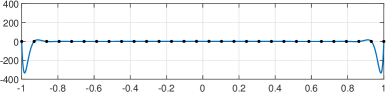
Fig. 1: Degree $29$ polynomial interpolant to the integrand $f(x)=1/(1+25x^{2})$ in $30$ equispaced points of $[-1,1]$. The Runge phenomenon of oscillations near the boundary leads to exponential divergence of the Newton–Cotes formula as $n\to\infty$.

Table 1: Errors in Newton–Cotes integration of polynomials $x^{k}$ and $T_{k}(x)$ with $n=30$. (Only even values of $k$ are shown since the integrals and errors are zero when $k$ is odd.) The errors for $T_{k}(x)$ are huge for $k\geq n$, a reflection of exponentially large quadrature weights of alternating signs.

$~{}~{}~{}k~{}~{}~{}$	$|E_{n}(x^{k})|$	$|E_{n}(T_{k}(x))|$
⋮	⋮	⋮
26	0	0
28	0	0
30	.0000007	399.5
32	.000005	2711.1
34	.00002	8923.1
36	.00004	18765.9
38	.00009	27812.9
⋮0	⋮	⋮

What is not well known is how this failure relates to the exactness principle, which we now consider in Table 1. With $n=30$, the Newton–Cotes formula integrates $x^{k}$ exactly for $k<30$, with $E_{n}(x^{k})=0$. A check of $E_{n}(x^{k})$ for $k\geq 30$ looks unexpectedly promising, with the errors coming out very small, smaller than one would have dreamed of for a quadrature formula of exactness degree $n-1$. However, this apparent good behavior is an illusion associated with the exponential ill-conditioning of monomial bases on $[-1,1]$. (Numerically speaking, $x^{k}$ has degree only $O(k^{1/2})$ for large $k$ [31].) Switching to the well-conditioned basis of Chebyshev polynomials $T_{k}(x)$ reveals that huge errors set in immediately at degree $k=30$.

Evidently for the Newton–Cotes formula, exact integration of degree $n-1$ polynomials has told us next to nothing about accuracy in integrating other functions.

3 Clenshaw–Curtis quadrature

The Clenshaw–Curtis formula, originating in 1960 [6], consists of integrating the degree $n-1$ polynomial interpolant through $n$ Chebyshev points

$$x_{j}=\cos(\kern 0.7ptj\pi/(n-1)),\quad 0\leq j\leq n-1.$$ (4)

This is the natural formula to apply in the context of Chebyshev spectral collocation methods for differential equations, and it is essentially the method by which Chebfun integrates a function, after first reducing it to a polynomial of sufficiently high degree [12]. Alternatively, nodes and weights can be computed explicitly in $O(n\log n)$ operations [48] and are available in Chebfun with the command [x,w] = chebpts(n).

Clenshaw–Curtis quadrature, like Newton–Cotes, has polynomial exactness degree $n-1$, but with none of the misbehavior as $n\to\infty$ since the weights are always positive. Pólya’s theory guarantees convergence for all $f\in C([-1,1])$ at a rate that follows the smoothness of $f$; if $f$ is analytic, the convergence is exponential [46, Theorems 19.3 and 19.4]. Thus the obvious expectation for Clenshaw–Curtis quadrature is that it should converge like Gauss quadrature, but at approximately half the rate, since Gauss has polynomial exactness degree $2n-1$.

This is not what happens. Gauss quadrature behaves as expected; the surprise is that Clenshaw–Curtis often converges at the Gauss rate too [46, Theorem 19.5]. Figure 2 shows a typical example. This effect was noted experimentally by Clenshaw and Curtis themselves, who wrote: “We see that the Chebyshev formula, which is much more convenient than the Gauss, may sometimes nevertheless be of comparable accuracy” [6]. A paper on the subject was published by O’Hara and Smith in 1968, who wrote: “The Clenshaw–Curtis method gives results nearly as accurate and Gaussian quadratures for the same number of abscissae” [32]. Subsequently the effect was mentioned in books of Evans [13] and Kythe and Schäferkotter [23] and then became more widely known through a paper of mine in 2008 [43].

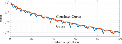
Fig. 2: Convergence of the Clenshaw–Curtis and Gauss quadrature formulas for the integrand $f(x)=\exp(-1/x^{2})$. The Gauss convergence is at the expected rate; the surprise is that Clenshaw–Curtis converges at this rate too.

O’Hara and Smith’s explanation of the unexpected accuracy of the Clenshaw–Curtis formula is that although its errors in integrating degree $k$ polynomials are nonzero for $k\geq n$, they are still very small for $n\leq k\ll 2n$. Note that this is precisely a failure of exactness as a guide to accuracy. The small errors are shown numerically in Table 2, a repetition of Table 1 (without the distracting $x^{k}$ column) for Clenshaw–Curtis. Figure 3 gives a visual picture of what is going on.

Table 2: Errors in Clenshaw–Curtis integration of polynomials $T_{k}(x)$ with $n=30$. Though nonzero, the errors for $n\leq k\ll 2n$ are small, of order $O(n^{-2})$. This is the explanation given by O’Hara and Smith [32] of the unexpected accuracy of Clenshaw–Curtis.

$~{}~{}~{}k~{}~{}~{}$	$|E_{n}(T_{k}(x))|$
⋮	⋮
26	0
28	0
30	0.0003
32	0.001
34	0.002
⋮0	⋮
54	0.1
56	0.7
58	2.0
60	0.7
⋮0	⋮

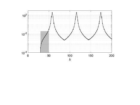
Fig. 3: Errors in Clenshaw–Curtis integration with $n=30$ of $T_{k}(x)$ as a function of even indices $k$. The shading highlights the small errors for $n\leq k\ll 2n$.

The effect shown in Table 2 and Figure 3 leads readily to an understanding of the surprising convergence rate of Clenshaw–Curtis quadrature as seen in Figure 2. Any Lipschitz continuous integrand $f$ will have an absolutely and uniformly convergent Chebyshev series,

$$f(x)=\sum_{j=0}^{\infty}a_{j}T_{j}(x),$$ (5)

from which it follows that the error (3) in Clenshaw–Curtis quadrature is

$$E_{n}(f)=\sum_{\scriptstyle{j=n}\atop\hbox{\scriptsize~{}$j$ even\kern 4.0pt}}^{\infty}a_{j}E_{n}(T_{j}).$$ (6)

If all the errors $E_{n}(T_{j})$ were of the same size $O(1)$, then $E_{n}(f)$ would depend just on the Chebyshev coefficients $\{a_{j}\}$, and this is approximately what happens in the regime $2n\leq j<\infty$. For the “shaded coefficients” $a_{j}$ with $n\leq j\ll 2n$, however, the errors $E_{n}(T_{j})$ are of size $O(n^{-2})$, and whether they contribute significantly to $E_{n}(f)$ depends on the rate of decrease of $\{a_{j}\}$ as $j\to\infty$, hence on the regularity of $f$. If $f$ is not analytic, as in the example of Figure 2, then $\{a_{j}\}$ decrease slowly enough that $a_{j}E_{n}(T_{j})$ is much smaller for $n\leq j\ll 2n$ than for $j\approx 2n$, making the contributions of the shaded coefficients to $E_{n}(f)$ negligible and producing the doubled-degree effect in its cleanest form. (There is still a complication, however, in that both Clenshaw–Curtis and Gauss converge at a rate faster than expected by one power of $n$ [52].) If $f$ is analytic, then $\{a_{j}\}$ decrease exponentially, and the terms $a_{j}E_{n}(T_{j})$ for $n\leq j\ll 2n$ are no longer negligible in comparison to the later ones, making the asymptotic convergence rate of Clenshaw–Curtis indeed half that of Gauss. For details, including the “kink phenomenon” observed for Clenshaw–Curtis quadrature of analytic integrands as the initial Gauss convergence rate cuts in half after a certain value of $n$, see [43, 50].

4 Gauss quadrature

Gauss quadrature, discovered by Gauss in 1814 [16], is defined by having the maximum possible polynomial degree of exactness, $2n-1$. This is achieved by taking the nodes $\{x_{j}\}$ as the roots of the degree $n$ Legendre polynomial $P_{n}$, and the name Gauss–Legendre is also used to distinguish this case from that of integrals in which a nonconstant weight function is introduced in (2) (next section). The weights for Gauss quadrature $\{w_{j}\}$ are all positive, and the formula is extremely effective in practice. Thanks to new algorithms introduced in the past 15 years and available with the Chebfun command [x,w] = legpts(n), the nodes and weights can be computed in a fraction of a second even when $n$ is in the millions [3, 12, 19].

Gauss quadrature is often described as optimal, but this is only precisely true in senses that are tied to polynomials. Specifically, it can be shown to be optimal by certain measures for integrating functions that are analytic in a Bernstein ellipse, an ellipse in the complex plane with foci $\pm 1$; see [36] and sections 4.9 and 6.9 of [4]. Analyticity in an ellipse, however, is a skewed form of smoothness, requiring more of a function in the middle of the interval than near the endpoints. Polynomials can resolve much faster wiggles near endpoints than in the interior [11], and Gauss quadrature (likewise Clenshaw–Curtis) inherits this property—as one sees intuitively from its strong clustering of sample points near the ends. For example, Gauss quadrature converges faster for the integrand $\sqrt{1.01-x}$ than for $\sqrt{0.1i-x}$, though the singularity of the first function is ten times closer to $[-1,1]$ than that of the second.

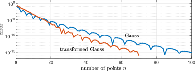
Fig. 4: Convergence of the Gauss formula and a conformally transformed Gauss formula $(\ref{Ing})$ for the same integrand $f(x)=\exp(-1/x^{2})$ as in Figure 2. While such transformed formulas have a limited role in practice, they illustrate that Gauss quadrature is not optimal.

From a user’s point of view, it would seem more natural to consider integrands with uniform smoothness across $[-1,1]$. In the analytic case, one might require analyticity in an $\varepsilon$-neighborhood of this interval, and quadrature formulas based on this assumption can be derived by transplanting Gauss quadrature via a conformal map $g$ with $g([-1,1])=[-1,1]$ of a Bernstein ellipse onto a cigar, or more simply, an infinite strip. Here the integral (2) becomes

$$I(f)=\int_{-1}^{1}g^{\prime}(s)f(g(s))\kern 0.5ptds,$$ (7)

and applying Gauss quadrature in the $s$ variable gives the transformed quadrature formula

$$I_{n}(f)=\sum_{j=1}^{n}w_{j}\kern 0.8ptg^{\prime}(s_{j})f(g(s_{j})).$$ (8)

An example is shown in Figure 4, with $g$ taken as the conformal map of the Bernstein ellipse with parameter $\rho=1.4$ (the sum of the semiminor and semimajor axes) onto an infinite strip. Such transplanted formulas were introduced in [20], and the conformal mapping idea goes back in the theoretical literature to Bakhvalov in 1967 [2] and was applied for spectral methods by Kosloff and Tal-Ezer [22]. As expected, the transformed quadrature nodes are much more uniformly distributed, with density ${\approx}\kern 0.7pt\pi/2$ times greater in the middle of the interval than for Gauss quadrature (not shown). In the limit $n\to\infty$ and $\rho\downarrow 1$, $\approx$ becomes $\sim\kern 0.7pt$.

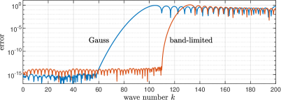
Fig. 5: Errors of $50$-point Gauss and band-limited quadrature formula integrating $\exp(ikx)$ for $k\in[-c,c\kern 0.5pt]$, with $c$ given by $(\ref{c})$. By this measure of integrating complex exponentials, the band-limited formula is notably more efficient.

A different approach to developing quadrature formulas with more uniform behavior, band-limited quadrature, is based on time-frequency analysis. Suppose one seeks a formula (1) that will integrate the functions $\exp(ikx)$ to high accuracy for all the wave numbers $k\in[-c,c\kern 0.5pt]$ for some $c>0$. Note that this is a continuum of wave numbers, not just the integer multiples of $\pi$ that would make the integrand 2-periodic. No choice of nodes and weights can integrate the continuum exactly, because its dimension is infinite. However, it has been known since the work of Slepian, Landau, and Pollak at Bell Labs in the 1950s and 1960s that the numerical dimension of this space is finite, just a bit larger than $2c/\pi$ [24, 25, 39]. Specifically, the singular values $\sigma_{j}$ of the bivariate kernel function $\exp(ikx)$ for $x\in[-1,1]$, $k\in[-c,c\kern 0.5pt]$ decrease exponentially for $j>2\kern 0.5ptc/\pi$. By applying the method known as generalized Gauss quadrature [5, 34] to an appropriate set of prolate spheroidal wave functions (PSWFs), one can develop quadrature rules that integrate these functions to high accuracy, as shown by Xiao, Rokhlin, and Yarvin [34, 53]. Later work has led to fast methods for calculating the nodes and weights of these formulas numerically [33, 34]. For $15$-digit accuracy, a good choice of $c$ (with the log correction term empirically determined; see [26] and [34, Thm. 2.4 and Prop. 17] for relevant theory) is

$$c=\pi n-12\log n\qquad(n\geq 8).$$ (9)

Figure 5 shows the accuracy of the band-limited quadrature formula with $n=50$ for approximating $\exp(ikx)$. Figure 6 repeats the convergence comparison of Figures 2 and 4.

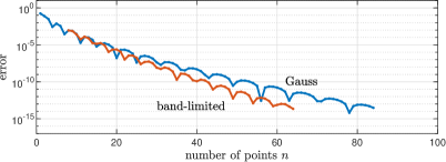
Fig. 6: Comparison of the Gauss and band-limited quadrature formulas for the integrand $f(x)=\exp(-1/x^{2})$, as in Figures 2 and 4. The curves stop at accuracy $10^{-13}$ because our computation of nodes and weights in the band-limited case is a few digits off machine accuracy, as was evident in Figure 5.

The term “band-limited quadrature” is convenient, but misleading. It is true that if one has an integrand that is band-limited to a known range $k\in[-c,c\kern 0.5pt]$, or nearly so, then these formulas will be excellent. But as equation (9) and Figure 6 illustrate, this is not the only potential application, and to say that these formulas are for integration of band-limited functions is not unlike saying that Gauss quadrature is for integration of polynomials.

Both of the alternatives to Gauss quadrature we have outlined in this section lead to the conclusion that the potential gain is a factor of $\pi/2$ in convergence rate. This is hardly enough to be very important in practice (at least in one space dimension [44, Fig. 11]), and I share the view, which is discussed with particular substance in section 6.9 of [4], that Gauss quadrature is the best choice known for general use.

5 Gauss–Hermite quadrature

Gauss–Hermite quadrature is the standard Gauss quadrature method for integrals over the whole real line. One supposes that a function $f$ is given and one wants to compute the integral

$$I=\int_{-\infty}^{\infty}e^{-x^{2}}\kern-2.0ptf(x)\kern 0.7ptdx,$$ (10)

which is (2) with $D=(-\infty,\infty)$ modified by the introduction of the weight function $\exp(-x^{2})$. The approximation will take the form (1) as usual, now with nodes $\{x_{j}\}$ in $(-\infty,\infty)$, and the Gauss–Hermite formula is defined by the nodes and weights taking the unique values such that $I(f)=I_{n}(f)$ whenever $f$ is a polynomial of degree $2n-1$. According to Gautschi [17], this method was introduced by Gourier in 1883 [18]. As with its unweighted progenitor discussed in the last section, Gauss–Hermite quadrature is intimately associated with orthogonal polynomials [40]. These are the Hermite polynomials $H_{0}(x)=1$, $H_{1}(x)=2x$, $H_{2}(x)=4x^{2}-2,\dots,$ which are orthogonal over $(-\infty,\infty)$ with respect to the inner product

$$\langle f,g\rangle=\int_{-\infty}^{\infty}e^{-x^{2}}\kern 2.0pt\overline{f(x)}\kern 1.0ptg(x)\kern 0.7ptdx.$$ (11)

The nodes $\{x_{k}\}$ are the roots of $H_{n}$, and as with Gauss–Legendre quadrature, algorithms have been developed to compute the nodes and weights with just $O(n)$ work [15, 42]. In Chebfun, [x,w] = hermpts(n).

In an application, one might start from an integrand $g(x)$ with Gaussian decay, so that $g$ can be written $g(x)=\exp(-x^{2})f(x)$ with $f(x)=O(1)$ on $(-\infty,\infty)$. It has been recognized from the beginning that there may be problems in practice with determining the right decay behavior. What if $g(x)$ looks more like $\exp(-\sigma x^{2})$ for some $\sigma\neq 1$, or decays in a non-Gaussian manner? We shall stay away from these questions and assume that $\exp(-x^{2})$ well approximates the shape of $g$.

Even in this most favorable setting, Gauss–Hermite quadrature is terribly inefficient as $n\to\infty$. For large $n$, most of the nodes lie far enough out along the real axis that their weights are minuscule; these terms then contribute negligibly to the sum (1) and can be thrown away! This curious phenomenon is known to experts, but I am unaware of any discussion in the literature of where the reasoning that led to the Gauss–Hermite formula has broken down. How can a formula that is optimal in a precise mathematical sense be so plainly suboptimal in practice? We shall first illustrate the problem, and then give an answer to this question.

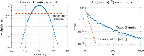
Fig. 7: A practitioner’s view of the inefficiency of Gauss–Hermite quadrature for large $n$. Many of the weights $w_{k}$ lie below machine precision—a fraction approaching $100\%$ as $n\to\infty$. The convergence rate is just root-exponential, whereas if one truncates to a finite interval and applies a standard quadrature method, it becomes exponential. The missing dots for the trapezoidal rule correspond to errors that are exactly zero in floating point arithmetic.

Figure 7 presents the inefficiency of Gauss–Hermite quadrature as a practitioner might encounter it. For the integrand we take $f(x)=\cos(x^{3})$, mixing energy at all wave numbers. The errors for Gauss–Hermite quadrature as a function of $n$ line up along a parabola on a semilog scale, corresponding to slow root-exponential convergence, and even with $n=1000$ the error is no smaller than $10^{-13}$. Yet $\exp(-x^{2})$ is of the order of $10^{-16}$ or less for $|x|>6$, so for practical purposes, this integral might as well be posed on the compact interval $[-6,6]$. Sure enough, the periodic trapezoidal rule applied on that interval shows much faster exponential convergence down to machine precision, and the convergence would be similarly fast for the Clenshaw–Curtis or Gauss formulas on $[-6,6]$. If $f(x)$ is changed to $\exp(-1/x^{2})$ as in Figure 2 (not shown), the convergence curves have about the same shapes though with about half the convergence rate.

The left side of Figure 7 shows how the Gauss–Hermite formula wastes its effort. For $n=100$, about half the weights lie below machine precision, 48 of them to be exact, and this fraction will increase with $n$. For $n=1000$, the number of weights below machine precision is 836. Clearly if $f$ is of order $1$, these function samples will not contribute usefully to the evaluation of the integral. Figure 8 illustrates the problem from another angle, plotting the Hermite functions

$$\psi_{n}(x)=H_{n}(x)\kern 0.7pte^{-x^{2}/2}(\sqrt{2\pi}\kern 0.7ptn!)^{-1/2},\quad n=0,1,\dots$$ (12)

for three values of $n$. These functions form a complete orthonormal set in the unweighted space $L^{2}(-\infty,\infty)$, and Gauss–Hermite quadrature implicitly expands $f$ in this basis. It is clear from the figure that this is going to be be an inefficient way of capturing the part of $f$ that matters to the integral, with $\psi_{32}$, for example, taking values of size $O(1)$ all across the interval $[-8,8\kern 0.8pt]$ even though $\exp(-8^{2}\kern 0.5pt)\approx 10^{-28}$.

Fig. 8: Hermite functions $(\ref{hermfuns})$, a complete orthonormal set in $L^{2}(-\infty,\infty)$ whose zeros are the Gauss–Hermite quadrature nodes $\{x_{k}\}$. The interval around $x=0$ where the amplitude is $O(1)$ broadens in proportion to $\sqrt{n}$, even though the integrand of $(\ref{gaussherm})$ decays at the rate $\exp(-x^{2})$.

Looking more deeply, there is no need for machine epsilon to be part of the discussion. For mathematical convergence of $I_{n}(f)$ to $I(f)$ when $I_{n}$ is defined by quadrature over a finite interval, the length of the interval will need to grow as $n\to\infty$, and the right choice for analytic functions $f(x)$ of size $O(1)$ on $(-\infty,\infty)$ is an interval of size $[-O(n^{1/3}),O(n^{1/3})]$, which balances a domain-truncation error of order $\exp(-n^{2/3})$ and a discretization error of the same order since the sample step size will be $h=O(n^{-2/3})$. (Discretization errors for the trapezoidal rule are quantified in [47]; the tool for such estimates is Cauchy integrals.) From this balance one can quantify the inefficiency of Gauss–Hermite quadrature, which places nodes approximately uniformly in $[-O(n^{1/2}),O(n^{1/2})]$ whereas $[-O(n^{1/3}),O(n^{1/3})]$ would suffice. Thus in effect only a fraction of order $n^{1/3}/n^{1/2}=n^{2/3}$ of the nodes are utilized, meaning that Gauss–Hermite quadrature employs more nodes than necessary by a factor of order $n^{1/3}$. The ratio increases to nearly order $n^{1/2}$ for nonanalytic functions $f$, where intervals growing just logarithmically rather than algebraically with $n$ are appropriate for balancing domain-truncation and discretization errors.

A theorem makes the point precise; the proof is given in the appendix.

Theorem 1.

Let $f(x)$ be analytic and bounded for $x\in(-\infty,\infty)$, and suppose $\exp(-x^{2})f(x)$ extends to a bounded analytic function in an infinite strip $-a<\hbox{\rm\kern 0.3ptIm\kern 1.0pt}x<a$. Let $L>0$ be fixed, and for each $n\geq 1$, let $I_{n}$ be the estimate of the integral $I$ of $(\ref{gaussherm})$ obtained by applying Gauss–Legendre, Clenshaw–Curtis, or trapezoidal quadrature on the truncated interval $[-Ln^{1/3},Ln^{1/3}\kern 0.7pt]$. Then for some $C>0$,

$$|I-I_{n}|=O(\exp(-Cn^{2/3})),\qquad n\to\infty.$$ (13)

In the literature, several authors have recommended adjustments to Gauss–Hermite quadrature that are related in one manner or another to truncating the domain to a finite interval such as $[-O(n^{1/3}),O(n^{1/3})]$. Mastroianni and Monegato and their coauthors have published a number of papers in this direction, focussing mainly on the analogous case of Gauss–Laguerre quadrature on $[\kern 0.5pt0,\infty)$ [28, 29] (see next section). Townsend, Trogdon and Olver note that for large $n$, only about $25\sqrt{n}$ of the weights $w_{k}$ are greater than the smallest machine number ${\approx}\kern 1.0pt10^{-308}$ in IEEE double precision, and recommend “subsampling” to retain only nodes and weights that will matter [42]. In unpublished work presented at a conference in 2018, Weideman showed how $O(\exp(-n^{2/3}))$ convergence with a particularly favorable constant can be obtained by applying the Gauss–Hermite formula with the weight function $\exp(-(n/2)^{1/3}x^{2})$ rather than $\exp(-x^{2})$ [49].

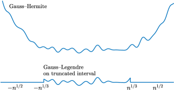
Fig. 9: Schematic illustration of the approximation problems $f\approx v\in V_{n}$ associated with Gauss–Hermite quadrature for $(\ref{gaussherm})$ and the alternative method of applying the Gauss–Legendre formula on a truncated interval $[-O(n^{1/3}),O(n^{1/3})]$, as in Theorem 1. The Gauss–Legendre method only needs to approximate $f$ on $[-O(n^{1/3}),O(n^{1/3})]$ to achieve an error $(\ref{1norm})$ of size $O(\exp(-O(n^{2/3})))$. The Gauss–Hermite method is effectively forced to approximate on a wider interval $[-O(n^{1/2}),O(n^{1/2})]$ just to keep the growth of polynomials under control.

However, the literature seems not to confront the conceptual question: what has gone wrong with the Gauss–Hermite notion of optimality? Here is an answer, summarized schematically in Figure 9. Suppose we have a quadrature formula for (10) that is exact for all functions $v$ in an $n$-dimensional space $V_{n}$. Its effectiveness will depend on how well $f$ can be approximated by functions $v\in V_{n}$ in the weighted $1$-norm

$$\|f-v\|=\int_{-\infty}^{\infty}e^{-x^{2}}|f(x)-v(x)|\kern 0.7ptdx.$$ (14)

(The study of weighted approximation problems on the real line was initiated by Bernstein [27].) Now Gauss–Hermite quadrature corresponds to taking $V_{n}$ as the space of polynomials of degree $n-1$, and this space is terribly inefficient for these weighted approximations since polynomials grow so fast as $|x|$ increases. For example, $x^{n}\exp(-x^{2})$ reaches a maximum of $(n/2\kern 0.3pte)^{n/2}$ at $x=\sqrt{n/2}$ — about $10^{6}$ for $n=20$ and $10^{17}$ for $n=40$. These huge numbers force a polynomial approximation to $f$ to pay attention to the whole interval $[-O(n^{1/2}),O(n^{1/2})]$, just to keep (14) under control. By contrast, when we apply Gauss–Legendre quadrature on a truncated interval $[-O(n^{1/3}),O(n^{1/3})]$, we are changing the approximation space $V_{n}$ to the set of polynomials of degree $n-1$ multiplied by the characteristic function of this interval. The approximation can focus just on the short interval, where much better accuracy is achievable.

6 Three more examples

We now mention briefly three further examples of quadrature formulas for which exactness proves an inaccurate guide to accuracy.

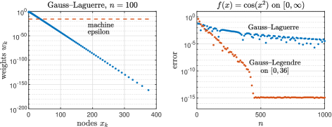
Fig. 10: Analogue of Figure 7 for Gauss–Laguerre quadrature, now with $f(x)=\cos(x^{2})$. As with Gauss–Hermite, many of the weights lie below machine precision and the convergence rate is just root-exponential; one does much better by discarding nodes and weights or truncating to a finite interval.

The first is Gauss–Laguerre quadrature, the analogue of (10) for integration over a semi-infinite interval:

$$I=\int_{0}^{\infty}\kern-1.0pte^{-x}f(x)\kern 0.7ptdx.$$ (15)

The design principle is that the nodes and weights should be such that the formula is exact when $f$ is a polynomial of degree $2n-1$. (In Chebfun, they can be computed by [x,w] = lagpts(n), an implementation of a fast algorithm of Huybrechs and Opsomer [21].) As with Gauss–Hermite quadrature, one finds that many of the weights are so small that the corresponding terms contribute negligibly to the result. For $n=100$ the minimal weight is $10^{-162}$ (decreasing exponentially with $n$), and just 38 weights lie above standard machine precision (a fraction increasing as $O(n^{1/2})$). For analytic $f$ of size $O(1)$ on $[\kern 0.5pt0,\infty)$ one has a domain-truncation error of size $\exp(-O(n))$ and a discretization error of order $\exp(-O(n^{1/2}))$, so the two are out of balance. By dropping nodes and weights or truncating to a shorter interval one can do much better, as illustrated in Figure 10. Truncated Laguerre formulas have been investigated in detail by Mastroianni and Monegato and their coauthors, though mostly for more general functions $f$ with the property that $e^{-x}f(x)$ may decay only algebraically as $x\to\infty$ [28, 29].

The second example involves the trapezoidal rule, that is, the approximation of an integral of a function $f(x)$ by the integral of its piecewise linear interpolant in a given set of sample points. Here the exactness principle is that $I_{n}(f)=I(f)$ whenever $f$ is a piecewise linear function with breaks at the nodes, which leads readily to an $O(h^{2})$ accuracy bound for any $f$ that is twice continuously differentiable. However, there is an important special case in which the convergence is much faster, which we exploited in Figure 7: when $f$ is smooth and periodic and the nodes are equally spaced. If $f$ is analytic, the convergence becomes exponential, at a rate $\exp(-O(n))$. The exactness principle based on piecewise linears fails to detect this, but it can be rescued (at least up to a Gauss factor of 2 attributable to aliasing) by the observation that for equispaced points, the piecewise linear interpolant has the same integral as a trigonometric interpolant. (Proof: in both cases the integral is equal to the mean of the sample data times the length of the interval.) For the trigonometric interpolant, fast convergence is readily proved via contour integrals or aliasing of Fourier series. Thus the special accuracy of the periodic equispaced trapezoidal rule can be understood by an exactness principle after all, so long as it is based on trigonometric interpolants instead of piecewise linears. For details see [47].

The third example concerns cubature formulas for integration in the $s$-dimensional hypercube $D=[\kern 0.7pt0,1]^{s}$. Following an idea introduced by James Clerk Maxwell in 1877 [30], one may approximate $I$ by the integral of a degree $d$ multivariate polynomial interpolant through a set of data values at $n$ points $x_{k}\in D$. For each $d\geq 0$, the dimension of the space of polynomials is $N={s+d\kern 1.0pt\choose s}$, and one would hope to be able to have $n\leq N$ nodes with positive weights. A theorem of Tchakaloff asserts that this is indeed possible (in greater generality, not just for a uniformly weighted integrals over a hypercube), even though a suitable set of nodes may be difficult to determine [41]. For extensive information about cubature formulas, see the survey article by Cools [7].

The difficulty with the exactness principle for cubature formulas concerns the limitations of multivariate polynomials as a guide to accuracy. The standard definition of the degree $d$ of a multivarate polynomial is the maximum 1-norm of its exponents; thus $p(x,y)=x^{3}y^{4}$, for example, has degree $d=7$. This definition has the property of isotropy (i.e., rotation-invariance) in $s$-space: if the variables are transformed by a rotation, the degree of a polynomial $p$ is unchanged. However, the hypercube is itself far from isotropic. The diagonals are $\sqrt{s}$ times longer than the diameters, and there are $2^{d}$ of them, so most of its volume is “in the corners” in the sense of lying outside the inscribed hypersphere. As a consequence, cubature formulas designed on Maxwell’s principle will behave anisotropically in $[\kern 0.7pt0,1]^{2}$, giving better accuracy for an integrand $f(x)=\varphi(x_{1})$ aligned along one axis, say, than for the same function rotated to $f(x)=\varphi((x_{1}+\cdots+x_{s})/\sqrt{s}\kern 1.0pt)$. For angle-independent resolution in the hypercube it would be necessary to base cubature formulas instead on the Euclidean degree, defined in terms of the 2-norm of the exponents. (For example, the Euclidean degree of $x^{3}y^{4}$ is $5$.) This effect was first pointed out in [44], and a theorem making it precise was published in [45]. Note the analogy to the discussion of Gauss quadrature on $[-1,1]$ in section 4. There the issue was translation-invariance, whereas here it is rotation-invariance.

It would be interesting to provide a numerical illustration of the suboptimality of standard cubature formulas. In preparing this article, however, I have come to realize that cubature formulas are not used much in practice, making it unclear exactly what nodes and weights might be appropriate for such a comparison. It appears that most multiple integrals are handled by essentially 1D methods such as tensor products, or by Monte Carlo methods and their relatives, or by other more specialized tools [10]. Nevertheless we can estimate how much efficiency should be lost, in principle, by building cubature formulas in the standard manner on the total degree. The number of coefficients needed to specify a polynomial of Euclidean degree $d$ is $d^{s}$ times the volume of an orthant of the $s$-hypersphere,

$$N_{\rm euclidean}={d^{s}\pi^{s/2}\over 2^{s}(s/2)!}\sim{d^{s}\over\sqrt{\pi s}\kern 0.7pt}\left({\pi e\over 2s}\right)^{\kern-1.5pts/2}\kern-2.0pt,$$

with the asymptotic approximation $\sim$ referring to the limit $d\to\infty$. To get the same resolution via the total degree would require the number of coefficients to be $d^{s}$ times the volume of the $s$-simplex expanded by $\sqrt{s}$ in each direction,

$$N_{\rm total}={d^{s}s^{s/2}\over s!}\sim{d^{s}e^{s}\over s^{s/2}\sqrt{2\pi s}\kern 0.7pt}\kern 1.0pt.$$

The inefficiency ratio associated with the standard design principle of cubature formulas is accordingly

$${N_{\rm total}\over N_{\rm euclidean}}={(s/2)!\over s!}\left({4s\over\pi}\right)^{\kern-1.5pts/2}\kern-2.0pt\sim{1\over\sqrt{2}\kern 0.7pt}\left({2\kern 0.5pte\over\pi}\right)^{\kern-1.5pts/2}\kern-2.0pt\approx(1.3)^{s-1}.$$

For dimensions $s=1$, $2$, $5$, $20$, and $40$ the ratios are about $1$, $1.27$, $2.83$, $171$, and $41104$.

7 Discussion

Quadrature theory is an edifice built over 200 years, featuring both detailed estimates and general theories. Often it may be hard to extract the important points, not least because valid estimates have a way of turning out to be far from sharp. In this article I have focussed on the theme of the exactness principle and how it may mislead, for this principle is the basis of how quadrature is presented to students in our textbooks. Unfortunately, on each particular topic, there are undoubtedly relevant results in the literature I am unaware of, for which I apologize.

Quadrature theory is not a hot research area nowadays; like complex analysis, it is a field that we use all the time but which has a way of seeming finished. A book that I have found particularly valuable is the 2011 monograph by Brass and Petras [4]. The opening chapter presents a “standard estimation framework” that elegantly makes precise the central question: given a quadrature formula, how can we speak quantitatively of its degree of optimality in integrating functions of particular classes? The book is full of results and references to detailed work on these problems. A definite integral is just one example of a linear functional, and the estimation framework for quadrature is related to wide-ranging theories including $n$-widths, information-based complexity, and optimal recovery. A recent contribution in this area is [9], and a textbook by Simon Foucart is forthcoming that will present links to data science and machine learning [14].

The exactness principle for designing quadrature formulas is algebraic, a matter of whether certain quantities are exactly zero or not. Quadrature, however, is a problem of analysis, concerned with whether certain quantities are small or not. It is to be expected that there will be some discrepancy between the two. Still, it is surprising that sometimes the discrepancy can be huge without our having fully noticed it, as in the case of Gauss–Hermite quadrature.

Appendix. Proof of Theorem 1

Proof.

Write $g(x)=\exp(-x^{2})f(x)$, and for fixed $L>0$ and each $n\geq 1$, let $J_{n}$ denote the interval $J_{n}=[-Ln^{1/3},Ln^{1/3}\kern 0.7pt]$. Since $f(x)$ is bounded for $x\in(-\infty,\infty)$, truncating $(-\infty,\infty)$ to $J_{n}$ introduces an error in the integral of $g$ of size $O(\exp(-Cn^{2/3}))$ for some $C$. Thus it is enough to show that the Gauss–Legendre, Clenshaw–Curtis, and trapezoidal approximations to the integral of $g$ over $J_{n}$ also have accuracy of this order.

For the trapezoidal rule, this follows from contour integral arguments as given in Section 5 of [47]. Theorem 5.1 of that section has additional assumptions concerning integrals of $g(x)$ along horizontal lines in the strip and decay of $g(x)$ to $0$ as $|x|\to\infty$, but these are only needed to derive an exact decay exponent. For our purposes, where the claim is just accuracy $O(\exp(-Cn^{2/3}))$ for some $C$, boundedness of $g$ is enough.

For the Gauss–Legendre and Clenshaw–Curtis formulas, the error estimate follows from Theorem 19.3 of [46]. That theorem asserts $O(\kern 0.7pt\rho^{-n})$ accuracy for integration of an analytic function on $[-1,1]$, assuming it can be analytically continued to a bounded analytic function in the Bernstein $\rho$-ellipse with foci $\pm 1$. Here, the ellipse must be scaled to foci $\pm Ln^{1/3}$, and for it to lie in the given fixed strip of analyticity as $n\to\infty$, we can take decreasing values $\rho=1+d\kern 0.5ptn^{-1/3}$ for a sufficiently small fixed value of $d$. The rescaled Theorem 19.3 of [46] now gives errors of size $O(n^{1/3}(1+d\kern 0.5ptn^{-1/3})^{-n})=O(\exp(-Cn^{2/3}))$, as required. ∎

References

- [1] A. P. Austin and L. N. Trefethen, Trigonometric interpolation and quadrature in perturbed points, SIAM J. Numer. Anal., 55 (2017), pp. 2113–2122.
- [2] N. S. Bakhvalov, On the optimal speed of integrating analytic functions, Comput. Math. Math. Phys., 7 (1967), pp. 63–75.
- [3] I. Bogaert, Iteration-free computation of Gauss–Legendre quadrature nodes and weights, SIAM J. Sci. Comput., 36 (2014), pp. A1008–A1026.
- [4] H. Brass and K. Petras, Quadrature Theory: The Theory of Numerical Integration on a Compact Interval, Amer. Math. Soc., 2011.
- [5] J. Bremer, Z. Gimbutas, and V. Rokhlin, A nonlinear optimization procedure for generalized Gauss quadratures, SIAM J. Sci. Comp., 32 (2010), pp. 1761–1788.
- [6] C. W. Clenshaw and A. R. Curtis, A method for numerical integration on an automatic computer, Numer. Math., 2 (1960), pp. 197–205.
- [7] R. Cools, Constructing cubature formulae: the science behind the art, Acta Numer. 6, (1997), pp. 1–54.
- [8] P. J. Davis and P. Rabinowitz, Methods of Numerical Integration, Academic Press, 1975.
- [9] R. DeVore, S. Foucart, G. Petrova, and P. Wojtaszczyk, Computing a quantity of interest from observational data, Constr. Approx., 49 (2019), pp. 461–508.
- [10] J. Dick, F. Y. Kuo, and I. H. Sloan, High-dimensional integration: The quasi-Monte Carlo way, Acta Numer., 22 (2013), pp. 133–288.
- [11] Z. Ditzian and V. Totik, Moduli of Smoothness, Springer Science & Business Media, 2012.
- [12] T. A. Driscoll, N. Hale, and L. N. Trefethen, Chebfun Guide, Pafnuty Publications, Oxford, 2014; see www.chebfun.org.
- [13] G. Evans, Practical Numerical Integration, Wiley, Chicehster, UK, 1993.
- [14] S. Foucart, Mathematical Pictures at a Data Science Exhibition, to appear.
- [15] A. Gil, J. Segura, and N. M. Temme, Fast, reliable and unrestricted iterative computation of Gauss–Hermite and Gauss–Laguerre quadratures, Numer. Math., 143 (2019), pp. 649–682.
- [16] C. F. Gauss, Methodus nova integralium valores per approximationem inveniendi, Comment. Soc. Reg. Gotting. Recent., 1814 (also in Gauss’s Werke, vol. III, pp. 163–196).
- [17] W. Gautschi, A survey of Gauss–Christoffel quadrature formulae, in EB Christoffel: The Influence of his work on Mathematics and the Physical Sciences, P. L. Butzer and F. Fehér, eds., Birkhäuser, Basel, 1981, pp. 72–147.
- [18] G. Gourier, Sur une méthode capable de fournir une valeur approchée de l’intégrale , C. R. Acad. Sci. Paris, 97 (1883), pp. 79–82.
- [19] N. Hale and A. Townsend, Fast and accurate computation of Gauss–Legendre and Gauss-Jacobi quadrature nodes and weights, SIAM J. Sci. Comput., 35 (2013), pp. A652–A674.
- [20] N. Hale and L. N. Trefethen, New quadrature formulas from conformal maps, SIAM J. Numer. Anal., 46 (2007), pp. 930–948.
- [21] D. Huybrechs and P. Opsomer, Construction and implementation of asymptotic expansions for Laguerre-type orthogonal polynomials, IMA J. Numer. Anal., 38 (2018), pp. 1085–1118.
- [22] D. Kosloff and H. Tal-Ezer, A modified Chebyshev pseudospectral method with an time step restriction, J. Comput. Phys., 104 (1993), pp. 457–469.
- [23] P. K. Kythe and M. R. Schäferkotter, Handbook of Computational Methods for Integration, Chapman and Hall/CRC, Boca Raton, FL, 2005.
- [24] H. J. Landau and H. O. Pollak, Prolate spheroidal wave functions, Fourier analysis and uncertainty—II, Bell Syst. Tech. J., 40 (1961), pp. 65–84.
- [25] H. J. Landau and H. O. Pollak, Prolate spheroidal wave functions, Fourier analysis and uncertainty—III: the dimension of the space of essentially time-and band-limited signals, Bell Syst. Tech. J., 41 (1962), pp. 1295–1336.
- [26] H. J. Landau and H. Widom, Eigenvalue distribution of time and frequency limiting, J. Math. Anal. Applics., 77 (1980), pp. 469–481.
- [27] D. S. Lubinsky, A survey of weighted approximation for exponential weights, arXiv preprint math/0701099, 2007.
- [28] G. Mastroianni and G. Monegato, Truncated Gauss–Laguerre quadrature rules, in Recent Trends in Numerical Analysis, D. Trigiante, ed., Nova Science, Hauppauge, NY, 2000, pp. 213–221.
- [29] G. Mastroianni and G. Monegato, Truncated quadrature rules over and Nyström-type methods, SIAM J. Numer. Anal., 41 (2003), pp. 1870–1892.
- [30] J. C. Maxwell, On approximate multiple integration between limits of summation, Proc. Cambridge Philos. Soc., 3 (1877), pp. 39–47.
- [31] D. J. Newman and T. J. Rivlin, Approximation of monomials by lower degree polynomials, Aequationes Math. 14 (1976), pp. 451–455.
- [32] H. O’Hara and F. J. Smith, Error estimation in the Clenshaw–Curtis quadrature formula, Comput. J., 11 (1968), pp. 213–219.
- [33] A. Osipov and V. Rokhlin, On the evaluation of prolate spheroidal wave functions and associated quadrature rules, Appl. Comput. Harmon. Anal., 36 (2014), pp. 108–142.
- [34] A. Osipov, V. Rokhlin, and H. Xiao, Prolate Spheroidal Wavefunctions of Order Zero: Mathematical Tools for Bandlimited Approximation, Springer, 2013.
- [35] J. Ouspensky, Sur les valeurs asymptotiques des coefficients de Cotes, Bull. Amer. Math. Soc., 31 (1925), pp. 145–156.
- [36] K. Petras, Gaussian versus optimal integration of analytic functions, Constr. Approx., 14 (1998), pp. 231–245.
- [37] G. Pólya, Über die Konvergenz von Quadraturverfahren, Math. Z., 37 (1933), pp. 264–286.
- [38] C. Runge, Über empirische Funktionen und die Interpolation zwischen äquidistanten Ordinaten, Z. Math. Phys., 46 (1901), pp. 224–243.
- [39] D. Slepian and H. O. Pollak, Prolate spheroidal wave functions, Fourier analysis and uncertainty—I, Bell Syst. Tech. J., 40 (1961), 43–63.
- [40] G. Szegő, Orthogonal Polynomials, 4th ed., Amer. Math. Soc., 1975.
- [41] V. Tchakaloff, Formules de cubatures mécaniques à coefficients non négatifs, Bull. des Sciences Math., 2nd series, 81 (1957), pp. 123–134.
- [42] A. Townsend, T. Trogdon, and S. Olver, Fast computation of Gauss quadrature nodes and weights on the whole real line, IMA J. Numer. Anal., 36 (2016), pp. 337–358.
- [43] L. N. Trefethen, Is Gauss quadrature better than Clenshaw–Curtis?, SIAM Rev., 50 (2008), pp. 67–87.
- [44] L. N. Trefethen, Cubature, approximation, and isotropy in the hypercube, SIAM Rev., 59 (2017), pp. 469–491.
- [45] L. N. Trefethen, Multivariate polynomial approximation in the hypercube, Proc. Amer. Math. Soc., 145 (2017), pp. 4387–4844.
- [46] L. N. Trefethen, Approximation Theory and Approximation Practice, Extended Edition, SIAM, 2019.
- [47] L. N. Trefethen and J. A. C. Weideman, The exponentially convergent trapezoidal rule, SIAM Rev., 56 (2014), pp. 385–458.
- [48] J. Waldvogel, Fast construction of the Fejér and Clenshaw–Curtis quadrature rules, BIT Numer. Math., 46 (2006), pp. 195–202.
- [49] J. A. C. Weideman, Gauss–Hermite vs trapezoidal rule, talk at SIAM Annual Meeting, Portland, Oregon, July 2008.
- [50] J. A. C. Weideman and L. N. Trefethen, The kink phenomenon in Fejér and Clenshaw–Curtis quadrature, Numer. Math., 107 (2007), pp. 707–727.
- [51] S. Xiang, Asymptotics on Laguerre or Hermite polynomial expansions and their applications in Gauss quadrature, J. Math. Anal. Appl., 393 (2012), pp. 434–444.
- [52] S. Xiang and F. Bornemann, On the convergence rates of Gauss and Clenshaw–Curtis quadrature for functions of limited regularity, SIAM J. Numer. Anal., 50 (2012), pp. 2581–2587.
- [53] H. Xiao, V. Rokhlin, and N. Yarvin, Prolate spheroidal wavefunctions, quadrature and interpolation, Inv. Problems, 17 (2001), pp. 805–828.