We present an overview of a proposal in relativistic proton-proton ($pp$) collisions emphasizing the thermal or kinetic freeze-out stage in the framework of the Tsallis distribution. In this paper we take into account the chemical potential present in the Tsallis distribution by following a two step procedure. In the first step we used the redundancy present in the variables such as the system temperature, $T$, volume, $V$, Tsallis exponent, $q$, chemical potential, $\mu$, and performed all fits by effectively setting to zero the chemical potential. In the second step the value $q$ is kept fixed at the value determined in the first step. This way the complete set of variables $T,q,V$ and $\mu$ can be determined. The final results show a weak energy dependence in $pp$ collisions at the centre-of-mass energy $\sqrt{s}=6$ GeV to 13 TeV. The chemical potential $\mu$ at kinetic freeze-out shows an increase with beam energy. This simplifies the description of the thermal freeze-out stage in $pp$ collisions as the values of $T$ and of the freeze-out radius $R$ vary only mildly over a wide range of beam energies.

1 Introduction

It has been estimated [1] that about 30,000 particles (pions, kaons, protons, antiprotons)) are produced in a central heavy ion collision at the Large Hadron Collider (LHC) at 5.02 TeV. Hence it is natural to use concepts from statistical mechanics to analyze the produced particles. This procedure has a long and proud history with contributions from three Nobel prize winners: E. Fermi [2, 3], W. Heisenberg [4] and L.D. Landau [5]. To quote Landau:

“Fermi originated the ingenious idea of considering the collision process at very high energies by the use of thermodynamic methods.”

This turned out to be useful also at much higher beam energies than those initially envisaged. The main ingredient in the hadron resonance gas model (referred to as thermal model here) is that all resonances listed in the Review of Particle Physics [6] are in thermal and chemical equilibrium. This reduces the number of available parameters and just a few thermodynamic variables characterize the system.

The chemical freeze-out stage is well understood and is strongly supported by experimental results (see e.g., [7] for a recent review) with a strong connection to results obtained using Lattice Quantum Chromodynamics (LQCD) as the chemical freeze-out temperature is consistent with the phase transition temperature calculated in LQCD. Indeed, for the most central Pb-Pb collisions, the best description of the ALICE data on yields of particles in one unit of rapidity at mid-rapidity was obtained for a chemical freeze-out temperature given by $T_{ch}=156.6\pm 1.7$ MeV [7, 8]. Remarkably, this value of $T_{ch}$ is close to the pseudo-critical temperature $T_{c}=156.5\pm 1.5$ MeV obtained from first principles Lattice QCD (LQCD) calculations [9], albeit with the possibility of a broad transition region [10].

For several decades, a well-established procedure using hydrodynamics [11] and variations thereof has existed to describe this stage. In this paper we review another possibility to describe the thermal freeze-out stage which has shown considerable potential especially to describe the final state in proton–proton (pp) collisions. Most of these approaches are based on variations of a distribution proposed by Tsallis about 40 years ago [12] to describe entropy by introducing an additional parameter called $q$. In the limit $q\rightarrow 1$ this reproduces the standard Boltzmann–Gibbs entropy. The advantage is that thermodynamic variables like temperature, energy density, pressure and particle density can still be used and thermodynamic consistency is maintained.

This paper is an extension of [13]. For completeness and for the convenience of the reader we have included the tables presented there and considerably improved on them, the inclusion of the NA61/SHINE [14] is new and contributes very much to the understanding of the energy dependence of the parameters, also all figures are new.

2 Thermal Freeze-Out

We will focus here on one particular form of the Tsallis distribution, satisfying thermodynamic consistency relations [15, 16] and given by:

$$E\frac{d^{3}N}{d^{3}p}=gVE\frac{1}{(2\pi)^{3}}\left[1+(q-1)\frac{E-\mu}{T}\right]^{-\frac{q}{q-1}},$$ (1)

where $V$ is the volume, $q$ is the Tsallis parameter, $T$ is the corresponding temperature, $E$ is the energy of the particle, $p$ is the momentum, $g$ is the degeneracy factor and $\mu$ is the chemical potential. In terms of variables commonly used in high-energy physics, rapidity $y$, transverse mass $m_{T}=\sqrt{p_{T}^{2}+m^{2}}$:

$$\frac{d^{2}N}{dp_{T}dy}=gV\frac{p_{T}m_{T}\cosh y}{(2\pi)^{2}}\left[1+(q-1)\frac{m_{T}\,\cosh\,y-\mu}{T}\right]^{-\frac{q}{q-1}}.$$ (2)

In the limit where the parameter $q$ tends to unity one recovers the well-known Boltzmann–Gibbs distribution (with $p_{T}$ being the particle transverse momentum):

$$\lim_{q\rightarrow 1}\frac{d^{2}N}{dp_{T}dy}=gV\frac{p_{T}m_{T}\cosh y}{(2\pi)^{2}}\exp\left(-\frac{m_{T}\,\cosh\,y-\mu}{T}\right).$$ (3)

The main advantage of Equation (2) over Equation (3) is that it has a polynomial decrease with increasing $p_{T}$ which is what is observed experimentally.

It was recognized early on [17] that there is a redundancy in the number of parameters in this distribution, namely the four parameters $T,V,q$ and $\mu$ in Equation $(\ref{YieldNonZeroMu})$ can be replaced by just three parameters $T_{0},V_{0},q$ with the help of the following transformation:

$$T_{0} = T\left[1-(q-1)\frac{\mu}{T}\right],\qquad\mu\leq\frac{T}{q-1},$$ (4)

$$V_{0} = V\left[1-(q-1)\frac{\mu}{T}\right]^{\frac{q}{1-q}},$$ (5)

leading to a transverse momentum distribution which can thus be written equivalently as

$$\frac{d^{2}N}{dp_{T}dy}=gV_{0}\frac{p_{T}m_{T}\cosh y}{(2\pi)^{2}}\left[1+(q-1)\frac{m_{T}\,\cosh\,y}{T_{0}}\right]^{-\frac{q}{q-1}},$$ (6)

where the chemical potential does not appear explicitly.

Corresponding to the volumes $V$ and $V_{0}$ defined in Equations (1) and (5) we also introduce the corresponding radii $R$ and $R_{0}$

$$V = \frac{4\pi}{3}R^{3},$$ (7)

$$V_{0} = \frac{4\pi}{3}R_{0}^{3}.$$ (8)

It is to be noted that most previous analyses have confused the two Equations (2) and (6) and reached conclusions that are incorrect, namely that at LHC energies, different hadrons, $\pi,K,p,...$ cannot be described by the same values of $T$ and $V$. As we will show this is based on using $T_{0}$ and $V_{0}$ and not $T$ and $V$. Many authors have followed this conclusion because at LHC energies equal numbers of particles and antiparticles are being produced and, furthermore, at chemical equilibrium, one has indeed $\mu=0$ MeV for all quantum numbers. However the equality of particle and antiparticle yields, at thermal freeze-out, only implies that e.g., $\pi^{+}$ and $\pi^{-}$ have the same chemical potential but they are not necessarily zero. We emphasize that Equations (2) and (6) carry a different meaning, notice the difference in parameters: $T_{0}$ is not equal to $T$ and neither is $V$ equal to $V_{0}$. Notice also that we do not have $\mu$ in Equation (6).

It is the purpose of the present paper to resolve this issue. The procedure we choose is the following:

1. Use Equation (6) to fit the transverse momentum distributions. This determines the three parameters $T_{0}$, $q$ and $V_{0}$.

2. Fix the parameter $q$ thus obtained.

3. Perform a new fit to the transverse momentum distributions using Equation (2) keeping $q$ as determined in the previous step. This determines the parameters $T$ and $V$ and the chemical potential $\mu$.

4. Check the consistency with Equations (4) and (5).

Each step in the fitting procedure thus involves only three parameters to describe the transverse momentum distributions. This procedure was presented in [13] and the present paper is an extension with more details in this paper, some of the entries in Table 2 have been corrected.

We emphasize that the chemical potentials at kinetic freeze-out (described here with a Tsallis distribution), are not related to those at chemical freeze-out. At chemical freeze-out, where thermal and chemical equilibrium have been well established the chemical potentials are zero. At kinetic freeze-out however, there is no chemical equilibrium and the observed particle-antiparticle symmetry only implies that the chemical potentials for particles must be equal to those for antiparticles. However, due to the absence of chemical equilibrium they do not have to be zero. The only constraint is that they should be equal for particles and antiparticles.

We remind the reader here of the advantage of using the above distribution as they follow a consistent set of thermodynamic relations (see e.g., [17]). From this, it is thus clear that the parameter $T$ can indeed be considered as a temperature in the thermodynamic sense since the relation below holds

$$T=\left.\frac{\partial E}{\partial S}\right|_{V,N},$$ (9)

where the entropy $S$ is the Tsallis entropy.

In the next section we include the chemical potential parameter in the Tsallis fits to the transverse momentum spectra. Previously, it was first noted by [17] that the variables $T,V,q$ and $\mu$ in the Tsallis distribution function Equation $(\ref{Yield})$ have a redundancy for $\mu\neq 0$ MeV and recently [18] considered the mass of a particle in place of chemical potential. This necessitates work on determining the chemical potential from the transverse momentum spectra.

3 Comparison of Fit Results

As mentioned in the introduction, we reproduce here for completeness the values extracted from the results published by the ALICE Collaboration [19, 20, 21, 22]. The data at the centre-of-mass energy $\sqrt{s}=0.9$ TeV had the smallest range in $p_{T}$ (for all the ALICE Collaboration results considered here), of about an order of magnitude less than the experimental data at $\sqrt{s}=2.76$ GeV and $\sqrt{s}=7$ TeV with ALICE.

In general the data were described very well; the figures showing the actual fits results are not included in this paper since they form part of previous publications. The least squares method was performed by the Minuit package [23] as part of the fitting procedure in the code. There was no manual selection in the choice of parameters, all parameters were initialized at the beginning and the code returned the best fit parameter values. We did not particularly fix the value of $T$ and tried to obtain the other parameters. In particular, the value of $\mu$ did not affect $V$.

We did not observe any trend which suggested a deterioration of the fits with the centre-of-mass energy. In Tables 1 and 2; we give the $\chi^{2}$ values. Comparing the values of $\chi^{2}$ from 2.76 to 7.0 TeV, in Tables 1 and 2, there was no clear trend with increasing energy.

Table 1: Fit results at $\sqrt{s}$ = 0.9 [19], 2.76 [20], 5.02 [21] and 7 TeV [21, 22], using data from the ALICE Collaboration using Equations (6) and (7).

$\sqrt{s}$ (TeV)	Particle	$R_{0}$ (fm)	$q$	$T_{0}$ (GeV)	$\chi^{2}$/NDF
0.9	$\pi^{+}$	4.83 $\pm$ 0.14	1.148 $\pm$ 0.005	0.070 $\pm$ 0.002	22.73/30
	$\pi^{-}$	4.74 $\pm$ 0.13	1.145 $\pm$ 0.005	0.072 $\pm$ 0.002	15.83/30
	$K^{+}$	4.52 $\pm$ 1.30	1.175 $\pm$ 0.017	0.057 $\pm$ 0.013	13.02/24
	$K^{-}$	3.96 $\pm$ 0.96	1.161 $\pm$ 0.016	0.064 $\pm$ 0.013	6.21/24
	$p$	42.7 $\pm$ 19.8	1.158 $\pm$ 0.006	0.020 $\pm$ 0.004	14.29/21
	$\bar{p}$	7.44 $\pm$ 3.95	1.132 $\pm$ 0.014	0.052 $\pm$ 0.016	13.82/21
2.76	$\pi^{+}+\pi^{-}$	4.80 $\pm$ 0.10	1.149 $\pm$ 0.002	0.077 $\pm$ 0.001	20.64/60
	$K^{+}+K^{-}$	2.51 $\pm$ 0.13	1.144 $\pm$ 0.002	0.096 $\pm$ 0.004	2.46/55
	$p+\bar{p}$	4.01 $\pm$ 0.62	1.121 $\pm$ 0.005	0.086 $\pm$ 0.008	3.51/46
5.02	$\pi^{+}+\pi^{-}$	5.02 $\pm$ 0.11	1.155 $\pm$ 0.002	0.076 $\pm$ 0.002	20.13/55
	$K^{+}+K^{-}$	2.44 $\pm$ 0.17	1.15 $\pm$ 0.005	0.099 $\pm$ 0.006	1.52/48
	$p+\bar{p}$	3.60 $\pm$ 0.55	1.126 $\pm$ 0.005	0.091 $\pm$ 0.009	2.56/46
7.0	$\pi^{+}+\pi^{-}$	5.66 $\pm$ 0.17	1.179 $\pm$ 0.003	0.066 $\pm$ 0.002	14.14/38
	$K^{+}+K^{-}$	2.51 $\pm$ 0.15	1.158 $\pm$ 0.005	0.097 $\pm$ 0.005	3.11/45
	$p+\bar{p}$	3.07 $\pm$ 0.41	1.124 $\pm$ 0.005	0.101 $\pm$ 0.008	6.03/43

Table 2: Fit results at $\sqrt{s}$ = 0.9 [19], 2.76 [20], 5.02 [21] and 7 TeV [21, 22], using data from the ALICE Collaboration with $q$ from Table 1 following Equations (2) and (8).

$\sqrt{s}$ (TeV)	Particle	$R$ (fm)	$\mu$ (GeV)	$T$ (GeV)	$\chi^{2}$/NDF
0.9	$\pi^{+}$	3.64 $\pm$ 0.21	0.055 $\pm$ 0.012	0.079 $\pm$ 0.002	3.66/30
	$\pi^{-}$	3.53 $\pm$ 0.21	0.059 $\pm$ 0.012	0.080 $\pm$ 0.002	2.18/30
	$K^{+}$	3.76 $\pm$ 0.33	0.029 $\pm$ 0.017	0.062 $\pm$ 0.003	5.31/24
	$K^{-}$	3.89 $\pm$ 0.35	0.003 $\pm$ 0.018	0.065 $\pm$ 0.003	3.38/24
	$p$	3.34 $\pm$ 0.27	0.233 $\pm$ 0.020	0.057 $\pm$ 0.007	7.44/21
	$\bar{p}$	3.93 $\pm$ 0.33	0.097 $\pm$ 0.024	0.065 $\pm$ 0.002	7.69/21
2.76	$\pi^{+}+\pi^{-}$	4.32 $\pm$ 2.68	0.022 $\pm$ 0.130	0.080 $\pm$ 0.019	20.48/60
	$K^{+}+K^{-}$	4.75 $\pm$ 0.03	$-$0.140 $\pm$ 0.008	0.075 $\pm$ 0.004	2.48/55
	$p+\bar{p}$	4.47 $\pm$ 5.50	$-$0.071 $\pm$ 0.253	0.077 $\pm$ 0.030	3.52/46
5.02	$\pi^{+}+\pi^{-}$	4.19 $\pm$ 2.64	0.038 $\pm$ 0.134	0.082 $\pm$ 0.021	20.14/55
	$K^{+}+K^{-}$	4.49 $\pm$ 0.03	$-$0.142 $\pm$ 0.009	0.078 $\pm$ 0.0005	1.52/48
	$p+\bar{p}$	4.00 $\pm$ 4.48	$-$0.075 $\pm$ 0.243	0.081 $\pm$ 0.031	2.56/46
7.0	$\pi^{+}+\pi^{-}$	3.67 $\pm$ 0.02	0.081 $\pm$ 0.141	0.081 $\pm$ 0.003	14.15/38
	$K^{+}+K^{-}$	3.80 $\pm$ 0.22	$-$0.098$\pm$ 0.014	0.082 $\pm$ 0.002	3.13/55
	$p+\bar{p}$	4.07 $\pm$ 0.27	$-$0.127$\pm$ 0.018	0.085 $\pm$ 0.002	6.03/43

The fits to the transverse momentum distributions were then repeated using Equation (2) but this time keeping the parameter $q$ fixed to the value determined in the previous section and listed in Table 1. The results are listed in Table 2, where we present the fit results for non-zero chemical potential for $pp$ collisions at four different beam energies by the ALICE Collaboration.

In the first case, we set the chemical potential as the mass of the respective particle and compare our results to [18] for $pp$ collisions at $0.9$ TeV with the CMS Collaboration, secondly we set the chemical potential as a free parameter to fit the data and analysis of the fit results and lastly, we calculated the chemical potential directly from Equation $(\ref{poland_mu})$.

In Table 3 we present the extracted values of $T,\,\,q\,,R$ and $\mu$ at four different energies with the CMS Collaboration.

Table 3: The extracted values of $T,\,\,q\,,R,\,\mu\,\mathrm{and}\,\,\chi^{2}/NDF$ parameters, using the data published in [24, 26, 25] for $pp$ collisions with the CMS experiment.

$\sqrt{s}$ (TeV)	Particle	$T$ (MeV)	$q$	$R$ (fm)	$\mu$ (MeV)	$\chi^{2}/NDF$
$0.9$ [24]	$\pi^{+}$	$77\pm 1$	$1.164\pm 0.004$	$0.070\pm 0.102$	$66\pm 4$	$8.111/18$
	$K^{+}$	$74\pm 1$	$1.158\pm 0.008$	$3.724\pm 0.126$	$-25\pm 9$	$2.123/13$
	$p^{+}$	$71\pm 1$	$1.139\pm 0.003$	$3.536\pm 0.105$	$94\pm 9$	$9.596/23$
$2.76$ [25]	$\pi^{+}$	$76\pm 1$	$1.189\pm 0.005$	$3.906\pm 0.100$	$80\pm 5$	$5.711/18$
	$K^{+}$	$78\pm 1$	$1.162\pm 0.008$	$3.883\pm 0.019$	$-5\pm 1$	$2.447/13$
	$p^{+}$	$67\pm 1$	$1.166\pm 0.004$	$3.508\pm 0.099$	$107\pm 9$	$27.43/23$
$7.0$ [25]	$\pi^{+}$	$77\pm 1$	$1.203\pm 0.005$	$3.994\pm 0.105$	$89\pm 1$	$14.29/18$
	$K^{+}$	$87\pm 1$	$1.152\pm 0.009$	$3.900\pm 0.135$	$-96\pm 11$	$2.074/13$
	$p^{+}$	$67\pm 1$	$1.184\pm 0.004$	$3.509\pm 0.099$	$84\pm 9$	$12.22/23$
$13.0$ [26]	$\pi^{+}$	$76\pm 2$	$1.215\pm 0.008$	$3.932\pm 0.157$	$88\pm 3$	$3.546/18$
	$K^{+}$	$88\pm 3$	$1.142\pm 0.0150$	$4.044\pm 0.27$	$-124\pm 22$	$1.828/13$
	$p^{+}$	$59\pm 1$	$1.213\pm 0.008$	$3.135\pm 0.130$	$191\pm 14$	$8.892/22$

In Figure 1 we compare the values for $T_{0}$ and $T$ at four different beam energies. The results obtained for $T$ were more stable for different particle types than the values obtained for $T_{0}$. We will come back to this with more detail later in this paper.

An interesting proposal to determine the chemical potential was made in [27], where the observation was made that the radius $R_{0}$ given in Table 1 is larger than the one obtained from a femtoscopy analysis [28] by a factor $\kappa$ estimated to be about 3.5, i.e.,

$$R_{\rm femto}\approx\frac{1}{\kappa}R_{0}.$$ (10)

Hence in [27] the suggestion is made to identify the corresponding volume $V_{\rm femto}$ with the volume $V$ appearing in Equation (1).

Hence

$$V_{0}\approx V\cdot\kappa^{3}.$$ (11)

Combining this with Equations $(\ref{T0})$ and $(\ref{V0})$ this leads to a chemical potential given by

$$\mu=\frac{T_{0}}{q-1}\left(\kappa^{3(q-1)/q}-1\right),$$ (12)

Hence, using this proposal, a knowledge of $T_{0}$ would lead to a determination of $\mu$.

We compared the resulting values of the chemical potential $\mu$ using this proposal [27] to the values using the procedure outlined above starting Equation (2) and concluded that the results are very different; hence, our results do not support this assumption and thus the volume $V$ appearing in Equation (2) cannot be identified with the volume determined from femtoscopy. The volume $V$ must be considered to be specific to the Tsallis distribution as is the case with all the other variables used in this paper.

A clearer picture of the energy dependence emerges when including results from the NA61/SHINE Collaboration [14] for $\pi^{-}$’s. The procedure outlined above was repeated in this case using the data published in [14], first we used Equation (6) and collect the results in Table 4. Next we fix the values of $q$ obtained this way and repeat the fits using Equation (1); the results are then collected in Table 5.

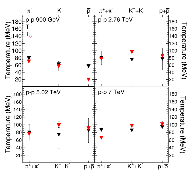
Figure 1: A comparison of the values of temperatures $T$ and $T_{0}$ of different hadron species for $pp$ collisions at $\sqrt{s}$ = 0.9 [19], 2.76 [20], 5.02 [21] and $7$ [22] TeV.

Table 4: The extracted values of $T_{0},\,\,q\,,R_{0}\,\,\mathrm{and}\,\,\chi^{2}/NDF$ parameters, using the data published in [14] for $pp$ collisions with the NA $61$ Collaboration.

$\sqrt{s}$ (GeV)	Particle	$T_{0}$ (MeV)	$q$	$R_{0}$ (fm)	$\chi^{2}/NDF$
$6.3$	$\pi^{-}$	$98\pm 6$	$1.042\pm 0.015$	$2.55\pm 0.14$	$4.454/15$
$7.7$	$\pi^{-}$	$95\pm 3$	$1.057\pm 0.008$	$2.72\pm 0.09$	$4.561/15$
$8.8$	$\pi^{-}$	$96\pm 2$	$1.055\pm 0.006$	$2.76\pm 0.06$	$8.423/15$
$12.3$	$\pi^{-}$	$95\pm 2$	$1.064\pm 0.006$	$2.90\pm 0.06$	$6.775/15$
$17.3$	$\pi^{-}$	$93\pm 3$	$1.069\pm 0.006$	$3.07\pm 0.08$	$2.176/15$

Table 5: The extracted values of $T,\,\,\mu\,,R\,\,\mathrm{and}\,\,\chi^{2}/NDF$ parameters, using the data published in [14] for $pp$ collisions with the NA $61$ Collaboration.

$\sqrt{s}$ (GeV)	Particle	$R$ (fm)	$\mu$ (GeV)	$T$ (GeV)	$\chi^{2}/NDF$
$6.3$	$\pi^{-}$	$2.451\pm 0.399$	$0.011\pm 0.046$	$0.098\pm 0.003$	$4.454/15$
$7.3$	$\pi^{-}$	$2.529\pm 0.223$	$0.020\pm 0.024$	$0.096\pm 0.002$	$4.561/15$
$8.8$	$\pi^{-}$	$2.548\pm 0.016$	$0.022\pm 0.002$	$0.097\pm 0.001$	$8.423/15$
$12.3$	$\pi^{-}$	$2.638\pm 0.171$	$0.026\pm 0.018$	$0.096\pm 0.001$	$6.776/15$
$17.3$	$\pi^{-}$	$2.785\pm 0.216$	$0.025\pm 0.021$	$0.095\pm 0.002$	$2.179/15$

The values for $T_{0}$ as a function of beam energy are shown in Figure 2. As one can see a fairly strong energy dependence was present when comparing the two sets of data.

However, this picture changes when plotting the temperature $T$ as a function of beam energy as shown in Figure 3. The energy dependence becomes weaker and the values of $T$ decrease with increasing beam energy from about 10 GeV all the way up to 13,000 GeV. A similar decrease of the kinetic freeze-out energy was also observed by the STAR collaboration [29] at the Brookhaven National Laboratory.

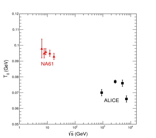
Figure 2: The energy dependence of the temperature parameter $T_{0}$. The triangular points are values of $T_{0}$ extracted from data in $pp$ collisions obtained by the NA61/SHINE [14] Collaboration for pions (see Table 4). The squares are the $T_{0}$ values in Table 1. All points were obtained by fits using Equation (6).

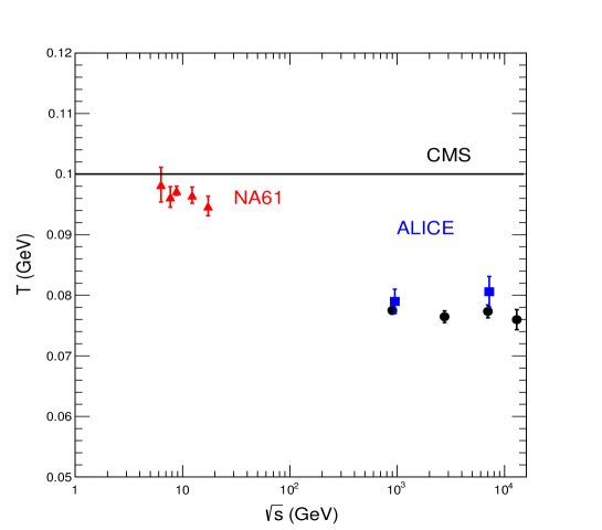
Figure 3: The energy dependence of the temperature $T$ for pions in $pp$ collisions. The triangular points are values of $T$ extracted from data in $pp$ collisions obtained by the NA61/SHINE [14] Collaboration for pions (see Table 5). The squares are the $T$ values in Tables  2 and 3. All points were obtained by fits using Equation (2). The straight line at $T$ = 0.1 GeV is there to guide the eye only.

Similarly when plotting the results obtained for the radius $R_{0}$ one sees a strong dependence on the beam energy as seen in Figure 4.

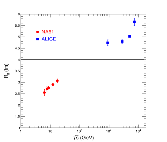
Figure 4: The energy dependence of the freeze-out radius $R_{0}$ of pions in $pp$ collisions. The round (red) points are obtained from fits to the results of the NA61/SHINE Collaboration [14] (see Table 4), the square points are for the ALICE Collaboration data (see Table 1). The straight line at $R_{0}$ = 4 fm is there to guide the eye only.

However, similarly to the case with the temperatures $T$ and $T_{0}$, the energy dependence s weakened when plotting the radius $R$ where only a very mild energy dependence could be noticed, see Figure 5.

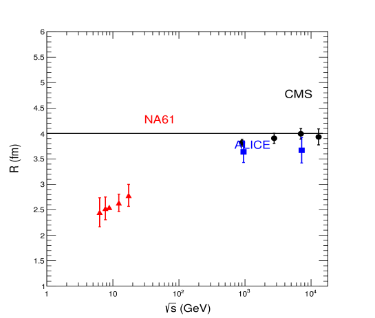
Figure 5: The energy dependence of the freeze-out radius $R$ of pions in $pp$ collisions. The round (red) points are obtained from fits to the results of the NA61/SHINE Collaboration [14] (see Table 5), the square (blue) points are for the ALICE Collaboration data (see Table 2), while the round (black) points are for the CMS Collaboration data (see Table 3). The straight line at $R$ = 4 fm is there to guide the eye only.

Finally the parameter which was most influenced by deviations from chemical equilibrium, namely the chemical potential $\mu$ which is shown in Figure 6. Here one sees a very clear increase with beam energy.

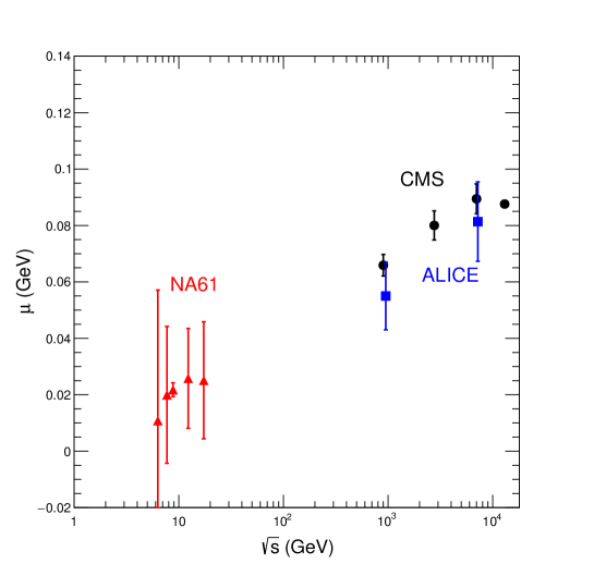
Figure 6: The energy dependence of the freeze-out chemical potential $\mu$ for pions in $pp$ collisions. The round (red) points are obtained from fits to the results of the NA61/SHINE Collaboration [14] (see Table 5), the square (blue) points are for the ALICE Collaboration data (see Table 2), while the round (black) points are for the CMS Collaboration data (see Table 3).

4 Conclusions

In this paper we have taken into account the chemical potential present in the Tsallis distribution Equation (1) by following a two step procedure. In the first step we used the redundancy present in the variables $T,V,q$ and $\mu$ expressed in Equations (4) and (5) and performed all fits using Equation (6), i.e., effectively setting the chemical potential equal to zero. The only variable which is common between Equations (1) and (6) is the Tsallis parameter $q$; hence, in the second step of our procedure we fixed the value of $q$ and performed all fits using Equation (1). This way we finally obtained the set of variable $T,V$ and $\mu$. The results are shown in several figures.  It is to be noted that $T$ and $R$ (as deduced from the volume $V$) show a weak energy dependence in proton-proton ($pp$) collisions at the centre-of-mass energies from $\sqrt{s}$ = 20 GeV up to 7 and 13 TeV. This is not the case for the variables $T_{0}$ and $V_{0}$. The chemical potential at kinetic freeze-out shows an increase with beam energy as presented in Figure 6. This simplifies the resulting description of the thermal freeze-out stage in $pp$ collisions as the values of $T$ and $R$ vary mildly over a wide range of beam energies.

References

- [1] D. Adamová et al., Phys. Lett. B 2017, 772, 567–577.
- [2] Fermi, E. Prog. Theor. Phys. 1950, 5, 570–583.
- [3] Fermi, E. Phys. Rev. 1951, 81, 683–687.
- [4] Heisenberg, W. Z. Phys. 1952, 133, 65.
- [5] Landau, L. Izv. Akad. Nauk Ser. Fiz. 1953, 17, 51–64.
- [6] M. Tanabashi et al. Review of particle physics. Phys. Rev. D 2018, 98, 030001.
- [7] A. Andronic, P. Braun-Munzinger, K. Redlich, J. Stachel, Nature 2018, 561, 321–330.
- [8] A. Andronic, P. Braun-Munzinger, B. Friman, P.M. Lo, K. Redlich, J. Stachel, Phys. Lett. B 2019, 792, 304–309.
- [9] A. Bazavov et al. Phys. Lett. B 2019, 795, 15–21.
- [10] S. Borsanyi, Z. Fodor, J.N. Guenther, R. Kara, S.D. Katz, P. Parotto, A. Pasztor, C. Ratti, K.K. Szabo, Phys. Rev. Lett. 2020, 125, 052001.
- [11] J. Sollfrank, P. Koch, U. W. Heinz, Phys. Lett. B 1990, 252, 256–264.
- [12] C. Tsallis, J. Statist. Phys. 1988, 52, 479–487.
- [13] J. Cleymans and M. Paradza, arXiv 2010, arxiv:2010.05565
- [14] N. Abgrall et al., Eur. Phys. J. C 2014, 74, 2794.
- [15] J. Cleymans and D. Worku, J. Phys. G 2012, 39, 025006.
- [16] J. Cleymans and D. Worku, Eur. Phys. J. A 2012, 48, 160.
- [17] J. Cleymans, G. Lykasov, A. Parvan, A. Sorin, O. Teryaev, D. Worku, Phys. Lett. B 2013, 723, 351–354.
- [18] Bíró, G.; Barnaföldi, G.G.; Biró, T.S. arXiv 2020, arXiv:2003.03278.
- [19] K. Aamodt et al., Eur. Phys. J. C 2011, 71, 1655.
- [20] B.B. Abelev et al., Phys. Lett. B 2014, 736, 196–207.
- [21] J. Adam et al., Phys. Lett. B 2016, 760, 720–735.
- [22] J. Adam et al., Eur. Phys. J. C 2015, 75, 226.
- [23] F. James and M. Roos, Comput. Phys. Commun. 1975, 10, 343.
- [24] S. Chatrchyan et al., JHEP 2011, 8, 86.
- [25] S. Chatrchyan et al., Eur. Phys. J. C 2012, 72, 2164.
- [26] A. M. Sirunyan et al. Phys. Rev. D 2017, 96, 112003.
- [27] M. Rybczynski and Z. Wlodarczyk, Eur. Phys. J. C 2014, 74, 2785.
- [28] T.C. Awes et al. Phys. Rev. D 2011, 84, 112004.
- [29] J. Adam et al. Phys. Rev. C 2020, 102, 034909.