Deep Anti-aliasing of Whole Focal Stack Using Slice Spectrum

Abstract

The paper aims at removing the aliasing effects of the whole focal stack generated from a sparse-sampled 4D light field, while keeping the consistency across all the focal layers. We first explore the structural characteristics embedded in the focal stack slice and its corresponding frequency-domain representation, i.e., the Focal Stack Spectrum (FSS). We observe that the energy distribution of the FSS always resides within the same triangular area under different angular sampling rates, additionally the continuity of the Point Spread Function (PSF) is intrinsically maintained in the FSS. Based on these two observations, we propose a learning-based FSS reconstruction approach for one-time aliasing removing over the whole focal stack. Moreover, a novel conjugate-symmetric loss function is proposed for the optimization. Compared to previous works, our method avoids an explicit depth estimation, and can handle challenging large-disparity scenarios. Experimental results on both synthetic and real light field datasets show the superiority of the proposed approach for different scenes and various angular sampling rates.

I Introduction

LIGHT field imaging [1] enables digital refocusing at different focal planes after the time of capture. Basically this is performed by integrating a light field over the angular domain, which corresponds to the slice operation in the frequency domain [2]. However, with a sparse angular sampling, i.e., the disparity between adjacent views is more than one pixel [3], there will be significant aliasing artifacts in the out-of-focus regions in the refocused images [4], as shown in Fig.1(a).

To enhance visual quality, many approaches [4, 5, 6, 7, 8, 9, 10] have been proposed to remove the aliasing effects based on view interpolation [7, 11, 12], depth-based filtering [3], or multi-scale fusion [4]. However, since most of these methods rely on depth estimation [13, 14], inaccurate depth maps will cause severe degradation in anti-aliasing performance. Moreover, existing methods only consider an individual refocused image, which is corresponding to a specific depth layer in the whole focal stack. Without taking all layers together into consideration, they could not provide consistent enhancement over the focal stack (as shown in Fig.18). Namely, along the axial direction in the focal stack, the PSF-continuity can not be maintained well. This will become more critical for the refocused images with large disparities or complex occlusions.

In the paper, we focus on exploring the structural characteristics embedding in the focal stack and its corresponding Fourier spectrum, named Focal Stack Spectrum (FSS). Different from the EPI (a 2D representation for a light field) where the slopes of the EPI lines vary with depths, for a given light field, the FSSs for different depths share the same cone-shaped pattern (as shown in the Fig.3). In other words, the energy distribution of the FSS locates within the same triangular area. Furthermore, the PSF-continuity is intrinsically maintained in the FSS. These important characteristics of the FSS make it possible to exploit a unified anti-aliasing scheme for whole depth contents.

Figure 1: Aliasing effect and aliasing-removed result. (a) Input with aliasing and the view count is $1\times 9$. (b) Anti-aliasing output by our method. From top to bottom, refocused image at a certain depth, focal stack slice along the red line, and corresponding FSS.

The main contributions of the paper are,

1) Two important characteristics of the frequency-domain representation for the light field focal stack are explored. The FSS can preserve the PSF-continuity and provide the same bounds of spectral support along the focal axis under different angular sampling rates.

2) A deep FSS-based anti-aliasing algorithm is proposed to perform one-time aliasing removal for all the refocused layers and meanwhile preserve the consistency across focal layers, only a rough disparity range estimation being needed.

3) A novel and robust conjugate-symmetric loss function is adopted in the U-Net for optimization.

II Related Work

II-A Light Field Refocusing

The 4D light field $L(u,v,x,y)$ [6, 15] records light rays in a 3D space, where $(u,v)$ and $(x,y)$ denote the ray’s intersections with the angular and spatial planes, respectively. So far, many studies have been done for analysing the 4D light field sampling characteristics and digital refocusing. In the spatial domain, by re-parameterizing the light rays and integrating them along the angular dimensions, the scene can be refocused [1]. In the Fourier domain, Ng [16] points out that the spectrum of a light field concentrates on a 3D manifold and each focal image could be synthesized by applying an inverse Fourier transform to a 2D slice in the manifold. After that, Dansereau et al. [9] extend the capability of refocus from a single depth layer to a volumetric range of depths by replacing the slice operation with a depth-dependent band-pass filter. It is worth noting that angular undersampling will cause severe aliasing artifacts and the above-mentioned methods can not remove this kind of aliasing.

II-B Anti-aliasing for Light Field Refocusing

Anti-aliasing usually requires either abundant angular sampling or appropriate filters. This problem has been widely studied in both spatial and frequency domains.

Spatial-domain methods. Most previous approaches rely on light field prefiltering. Levoy and Hanrahan [6] employ a prefiltering to reduce the spatial artifacts. However, the prefiltering inevitably introduces over-smoothness in the focused areas. In order to mitigate the over-smoothness issue, some depth-based methods are proposed to remove the aliasing. Levin et al. [17] propose to use the mixture-of-Gaussians derivative priors to recover a nearly aliasing-free light field given the scene depths. Chang et al. [7] propose an anti-aliasing algorithm by interpolating angular sampling within each sampling interval using depth information. Lin et al. [13] analyse the symmetry characteristic of the focal stack slice in the spatial domain and prove it is possible to use depth-based light field rendering to reduce the aliasing. All these methods need accurate scene depths. Recently, with the development of light field reconstruction techniques [12, 18, 19, 20], many light field angular super-resolution methods have been proposed to reduce the aliasing. Kalantari et al. [11] propose two convolutional neural networks to estimate the depth and color of each viewpoint sequentially. Wu et al. [12] remove the aliasing by performing angular super-resolution on the EPI. Yeung et al. [18] propose a learning-based algorithm to reconstruct a densely-sampled LF rapidly and accurately from a sparsely-sampled LF in one forward pass. Srinivasan1 et al. [20] predict the Multiplane Image (MPI) scene representation from a narrow baseline stereo pair, which can be used for view synthesis. Mildenhall et al. [19] propose to render novel views by blending adjacent local light fields. These techniques require solving the scene reconstruction problem, which is a traditional challenge. Without reconstruction, Bishop et al. [21] eliminate the aliasing by fusing multiview information. By analysing the angular aliasing model in the spatial domain, Xiao et al. [4] first detect the aliasing contents and then use lower-frequency terms of decomposition to remove the angular aliasing at the refocusing stage. Dayan et al. [10] propose a convolutional neural network to remove the aliasing effects from a sparse light field.

Frequency-domain methods. Isaksen et al. [1] propose a frequency-planar light field filter. Chai et al. [3] conduct a comprehensive analysis on the trade-off between sampling density and depth resolution in the frequency domain and reconstruct the EPI spectral using depth filters. Ng [16] suggests that band-limited filtering in the frequency domain and slicing can effectively inhibit the aliasing effects. In terms of view reconstruction, Le Pendu et al. [22, 23] present a Fourier Disparity Layer (FDL) representation for light fields. Once the layers are known, they can be simply shifted and filtered to produce different viewpoints to remove the aliasing. Shi et al. [24] propose to complete the angular spectrum of a light field in the continuous Fourier domain. Vagharshakyan et al. [25] iteratively compensate the high frequency spectrum of a sparse EPI representation in shearlet domain.

However, all these methods have their specific limitations. Prefiltering techniques can eliminate aliasing only while the focused areas are also over-smoothed. Depth and view reconstruction based techniques are prone to depth or reconstruction errors. When the refocused depth is far away from the original focused depth, the aliasing is aggravated. Moreover, all these methods tackle each refocused image individually so that they can not provide a PSF-continuous aliasing-removed focal stack (as shown in Fig.18). Different from these methods, the proposed FSS representation enables the same cone-shaped distribution pattern in the frequency domain shared by different scenarios, which provides a unified depth-independent solution for generating the PSF-continuous anti-aliasing focal stack in one single pass.

III Focal Stack Spectrum

In this section, we first elucidate the way to obtain the FSS from a light field, and then analyse the characteristics of the FSS. Without loss of generality, a 2D EPI instead of a full 4D one is used here to deliver good demonstrations.

III-A Definition of FSS

Figure 2: Analysis for the EPI in the $u$-$x$ space, the focal stack in the $f$-$x$ space and the FSS in the $\omega_{f}$-$\omega_{x}$ space. (a)-(c) Original and sheared EPIs with different parameters. (d) Aliased focal stack. (e) Continuous focal stack. (f) Fourier spectrum of (d). For better visualization, only one single pixel $P$ is considered here.

For better understanding, the notations used in the paper are given in Tab. I. $E(u,x)$ denotes a 2D EPI of a 4D light field, where $u$ and $x$ refer to the angular and spatial dimensions, respectively. $E_{d}(u,x)$ denotes the sheared EPI at a specific disparity $d$,

$$\small E_{d}(u,x)=E(u,x+d(u-u_{ref})),$$ (1)

where $u_{ref}$ refers to the reference view. Once the sheared EPI with an arbitrary disparity $f\in[d_{min},d_{max}]$ is integrated for all views, the focal stack $F(f,x)$ is formed,

$$\small F(f,x)\!=\!\int\!\!E(u,x+f(u-u_{ref})){d}u.$$ (2)

Subsequently, the Fourier form of $F(f,x)$ is

$$\small\mathcal{F}(\omega_{f},\omega_{x})=FT(F(f,x)),$$ (3)

where $FT(\cdot)$ refers to the 2D Fourier transform operator. Specifically, the view number of the given light field is $N_{u}$.

TABLE I: Notations used in the paper

Term	Definition
$E(u,x)$	A 2D EPI of a 4D light field
$E_{d}(u,x)$	Sheared EPI at the disparity $d$
$u$	Angular coordinate
$x$	Spatial coordinate
$f$	Focal layer’s disparity
$F(f,x)$	Focal stack formed by $E(u,x)$
$\mathcal{F}(\omega_{f},\omega_{x})$	Focal stack spectrum
$FT(\cdot)$	Fourier transform operator
$u_{ref}$	Reference view
$N_{u}$	View number

III-B Characteristics of Focal Stack and Its Spectrum

III-B1 Aliasing and Defocus in the Focal Stack

Sparse views and aliased focal stack. Fig.2(a) shows an EPI with 5 views, where the baseline between neighboring views is defined as 1 unit. A 3D point is imaged as $P_{0},P_{1},P_{2},P_{3},P_{4}$ in different views. The disparity of $P$ is $d^{*}$. When the EPI is sheared using Eqn.1 with $d=d^{*}$, the disparity of $P$ becomes $0$ (Fig.2(b)). When the EPI is sheared with parameter $\alpha$, compared with the original EPI (Fig.2(a)), the shearing parameter $d=d^{*}+\alpha$ and the current disparity of $P$ becomes $-\alpha$ now (Fig.2(c)).

By accumulating these three EPIs along the angular axis using Eqn.2, we get three focal images, i.e., the three dotted lines in Fig.2(d). It is noticed that the distribution of $P$ varies from slice to slice. Originally, the imaging of $P$ is aliased and $P$ is decomposed as $P_{0}$, $P_{1}$, $P_{2}$, $P_{3}$, $P_{4}$. When the EPI is sheared with $d=d^{*}$, these five pixels are converged into one pixel $P$. In the third slice, $P$ is aliased again and decomposed as $P_{0}^{\prime}$, $P_{1}^{\prime}$, $P_{2}^{\prime}$, $P_{3}^{\prime}$, $P_{4}^{\prime}$. The imaging range of $P$, i.e., the distance from $P_{0}$ to $P_{4}$ or $P_{0}^{\prime}$ to $P_{4}^{\prime}$, can be calculated by

$$\small l_{P_{0},P_{4}}=|\alpha|(N_{u}-1).$$ (4)

Repeat the above shearing process with the sampling interval $\Delta\alpha$ to construct a focal stack (Fig.2(d)). The distribution of $P$ forms a cone-shaped pattern in the focal stack, i.e., the similar triangles $\triangle PP_{0}P_{4}$ and $\triangle PP_{0}^{\prime}P_{4}^{\prime}$. The apex angle $\varphi$ of such a triangle is

$$\varphi=2\arctan(\frac{1}{2}\Delta\alpha(N_{u}-1)).$$ (5)

The slope of each component $PP_{i}$ in the $f-x$ coordinates of Fig.2(d) could be computed by

$$Slope(PP_{i})=\frac{1}{\Delta\alpha(u_{i}-u_{ref})}.$$ (6)

Dense views and defocused focal stack. By inserting more views between neighboring views $u_{i}$ and $u_{i+1}$ in Fig.2(a)(b)(c), more lines appear between the line $PP_{i}$ and $PP_{i+1}$ in Fig.2(d). When the views are dense enough, the aliasing becomes defocus blur (Fig.2(e)). The defocus diameter of $P$ could also be calculated using Eqn.4. Noting that, since the baseline between neighboring views is scaled by $\frac{1}{M+1}$ when inserting $M$ views, the defocus diameter in Fig.2(e) is equal to the aliasing distance in Fig.2(d). The apex angle $\varphi$ does NOT change (the same cone-shaped pattern still exists, as shown in Fig.2(e)).

Continuous focal stack. The above analysis focuses on the focal stack with a sampling interval $\Delta\alpha$. When the focal stack is constructed in the continuous domain, Eqns.5 and 6 could be rewritten as

$$\varphi_{con}=2\arctan(\frac{1}{2}(N_{u}-1)).$$ (7)

$$Slope(PP_{i})_{con}=\frac{1}{u_{i}-u_{ref}}.$$ (8)

According to Eqns.5-8, we get the following observations,

1. The shapes of defocus blur or aliasing lines are determined by the refocus parameter $\Delta\alpha$ and the view index, which is independent of depth.

2. All aliasing lines from the same view have the same slope (as the lines $PP_{i}$ shown in Fig.2 (d)).

Figure 3: Comparisons of a light field under different angular sampling rates. From top to bottom: EPI and its spectrum, focal stack slice and corresponding FSS. From left to right: (a) Dense sampling with $121$ views. (b) $5\times$ downsampling. (c) $15\times$ downsampling.

III-B2 Aliasing and Defocus in the FSS

Given a focal stack formed from a $N_{u}$-view light field, there are $N_{u}$ frequency lines in the FSS according to the property of the Fourier transformation [26] : each line corresponds to a specified view and more views lead to more lines. Consequently, the FSS also has the following properties,

1. The shape of the FSS is determined by the refocus parameter $\Delta\alpha$ and the view index, which is independent of depth.

2. According to the property of the Fourier transformation [27], the FSS is conjugate symmetric.

III-C EPI Spectrum vs. FSS

In this section, we will analyse the differences between the EPI spectrum and the proposed FSS. Insufficient sampling will result in repeated and overlapped aliasing patterns in the Fourier spectrum of the EPI [3, 19, 20] and the bound on the spectral support depends on the depth range ($[z_{min},z_{max}]$). While FSS is the integral result in the frequency domain. With changing focus depths, all contents from the same view will be gathered in the same line in the FFS (refer to Sec.III-B).

Fig.3 shows the comparisons between the aliased EPI spectrum and the aliased FSS under different sampling rates. Taking a closer look at these two spectra, more repeating areas appear in the EPI spectrum with respect to the decrease in the number of views, while the structural distribution of the FSS still remains. Additionally, there is a one-to-one correspondence between the line in the FSS and the view when $\Delta\alpha$ is fixed. As shown in Fig.3(c) (the rightmost column), 9 views in the EPI correspond to 9 lines in the FSS.

Because the EPI spectrum overlaps in the frequency domain, appropriate low-pass filtering is needed to remove the overlapping of aliased components during reconstruction or rendering. However, these low-pass filters tend to result in an over-smoothness in the focused regions. By contrast, the FSS has no overlapping spectrum so that there is no such “spectrum isolation” problem in the proposed solution. As discussed in Sec.III-B2, insufficient angular sampling causes aliasing effects in the focal stack. Considering the properties that each line of the FSS corresponds to a specific view and more views lead to more lines, the anti-aliasing problem could be formulated as a spectrum completion one based on the FSS.

Fig.4(c) shows the anti-aliasing result at $15\times$ downsampling using a low-pass filter on the EPI, and Fig.4(d) shows the result using the proposed FSS-based deep anti-aliasing algorithm. The EPI-based result is over-smoothed at the focused points (the area pointed by the green arrow). The proposed method not only eliminates the aliasing effects but also maintains the sharpness of focused points and edges.

Figure 4: $15\times$ downsampling anti-aliasing results on different focal layers. (a) GT (1$\times$ $121$ views). (b) Input (1$\times$ 9 views). Anti-aliasing results by performing (c) low-pass filtering on the EPI and (d) our FSS-based deep anti-aliasing algorithm.

Figure 5: The pipeline of the proposed FSS-based deep anti-aliasing algorithm.

IV Proposed Method

As mentioned in Sec. III-B, aliasing effects are caused by insufficient angular sampling and there is a relationship between the number of views and the FSS. As a result, the anti-aliasing problem could be modeled as a spectrum completion one. The pipeline of the proposed FSS-based anti-aliasing algorithm is shown in Fig.5.

Specifically, the aliasing focal stack $F_{a}(f,x)$ is obtained from the undersampled EPI using Eqn.2. Then the Fourier transform operator $FT(\cdot)$ is applied to obtain the FSS $\mathcal{F}_{a}(\omega_{f},\omega_{x})$. Finally, a CNN $\phi$ parameterized by $\sigma$ is proposed to reconstruct the aliasing-removed FSS $\mathcal{F}(\omega_{f},\omega_{x})$ from $\mathcal{F}_{a}(\omega_{f},\omega_{x})$,

$$\underset{\sigma}{\arg\min}\left\{\left\|\mathcal{F}_{gt},\phi_{\sigma}(\mathcal{F}_{a})\right\|\right\},$$ (9)

where $\mathcal{F}_{gt}$ is the ground truth FSS.

As shown in Fig.6, to deal with complex number inputs, a dual-stream U-Net [28] is designed. The power spectrum and the phase angle are firstly fed into two sub-networks respectively. Then the generated features are combined using the Euler’s formula to obtain the real and imaginary parts, which are concatenated and fed to another network for optimization. Fig.7 shows more details of the adopted U-Net architecture.

Figure 6: The structure of the proposed FSS completion network.

Figure 7: The U-Net architecture adopted in the paper [28].

The loss function is,

$${loss}=\|\mathcal{F}-{\mathcal{F}_{gt}}\|_{2}+\lambda\cdot{loss}_{s},$$ (10)

where ${loss}_{s}$ constrains the conjugate symmetry of the reconstructed FSS. The scalar $\lambda$ is set to 1.5 for balancing the two loss terms,

$$\small{loss}_{s}=\frac{1}{N_{C}W}\sum\limits_{i=0}^{N_{C}-1}\sum\limits_{j=0}^{W-1}\left|\mathcal{F}(\omega_{i},\omega_{j})-{\mathcal{F}^{*}(-\omega_{i},-\omega_{j})}\right|,$$ (11)

where $|\cdot|$ refers to the norm of a complex number, $*$ indicates the standard conjugate operation on a complex number. $N_{C}$ and $W$ denote the number of refocus layers and the image width respectively.

The complete FSS-based deep anti-aliasing algorithm is summarized in Algorithm 1.

Algorithm 1 The FSS-based deep anti-aliasing algorithm

0:    An angularly undersampled 3D light field $L(u,x,y)$, with $N_{u}$ views of $H\times W$ pixels.

0:    An anti-aliasing 3D focal stack.

1:  for $y=1$ to $H$ do

2:     Get the 2D light field $E(u,x)$.

3:     Obtain the focal stack slice $F_{a}(f,x)$ by Eqn.2.

4:     Get the aliasing FSS $\mathcal{F}_{a}(\omega_{f},\omega_{x})$ by Eqn.3.

5:     Reconstruct the aliasing-reduced FSS $\mathcal{F}(\omega_{f},\omega_{x})$ with the dual-stream U-Net.

6:     Perform an inverse Fourier transform on $\mathcal{F}(\omega_{f},\omega_{x})$.

7:  end for

8:  Get the anti-aliasing 3D focal stack.

V Experimental Results

In this section, we demonstrate the performance of the proposed FSS-based anti-aliasing algorithm on both synthetic and real light fields. The robustness of the proposed method is firstly validated on light fields with different sampling rates. Then, an ablation experiment is conducted to verify the effectiveness of the conjugate-symmetric loss. Finally, both the quantitative and qualitative comparisons with SOTAs are provided to demonstrate the superiority of the proposed method. Additional experiments on light fields captured from a camera array further verify the generalization of the proposed method.

V-A Datasets and Implementation Details

To train and verify the proposed network, both synthetic and real light fields are used. For synthetic data, 6 light fields are rendered using the light field automatic generator [29] and POV-Ray [30], of which 4 for training and 2 for testing. For real data, the high angular resolution light field datasets [31] are used, of which 10 for training and 2 for testing. Note that only $121$ views are used. Additionally, the Stanford [32] and the Disney [33] light fields are used to verify the performance of the proposed method on unseen light fields captured by a camera array. Tab. II shows the details of these light field datasets. Notice that, the spatial resolutions for Couch and Church light fields ($2670\times 4020$ and $2622\times 4007$ respectively) are resized in our experiments.

Details of light field scene selection. Fig.8 shows the reference views in our synthetic light field datasets. In the synthetic datasets, the scenes Pot-cube (Fig.8(a)) and Tree (Fig.8(b)) are used for testing, since the occlusions in these two scenes are more complex. In the real light field datasets [31], the scenes Bicycle and Hydrant are selected for testing due to the larger disparity ranges, which could better verify the generalization of the proposed method under different scenes. In the Disney datasets [33], the scenes Couch and Church are selected for testing since they are motion-free and exhibit larger disparities. Besides, we also choose the StillLife scene from the HCI datasets [34] for testing. Different from other datasets which provide sufficient views, the angular sampling of StillLife is inadequate, i.e., there is aliasing in refocused images even all the views are used. The proposed method is capable of eliminating the implied aliasing effect in this scene, as shown in Fig.1.

Figure 8: Reference views of our synthetic light field datasets.

In order to verify the capability of the proposed method for large disparity, we conduct experiments with different angular sampling rates. At present, only single direction disparity is concerned, so the 2D EPI can be used to represent the input light field. Fig.9 shows details of testing light fields under $5\times$ and $15\times$ downsampling scales. For each light field, the focal stack $F(f,x)$ is constructed by performing refocusing operations 199 times with $\Delta\alpha=0.01$. Tab. II shows the ranges of refocus operation ($d$).

Figure 9: EPIs under different view downsampling rates. (a) Reference view. (b) Original EPI. (c) $5\times$ downsampling. (d) $15\times$ downsampling.

The network converges after 150 epochs where each epoch contains 30 iterations. The Adam optimizer [35] is used for iterative optimization. The learning rate is initially set to 0.001. The first and second moments of the gradients are set to 0.9 and 0.99 respectively to enable adaptive learning rates. The network is implemented using the TensorFlow framework with 7 GTX 1080Ti GPUs.

TABLE II: Details of light fields evaluated in the experiments.

Dataset	Rang of $d$	Angular Res.	Spatial Res.
Syn. LF	[-1.00,0.98]	$1\times 121$	$526\times 526$
Real LF [31]	[-1.00,0.98]	$1\times 121$	$376\times 526$
Couch [33]	[-2.60,-0.60]	$1\times 101$	$628\times 1024$
Church [33]	[-1.45,-0.53]	$1\times 101$	$670\times 1024$
Lego [32]	[-1.00,0.98]	$1\times 17$	$1024\times 1024$

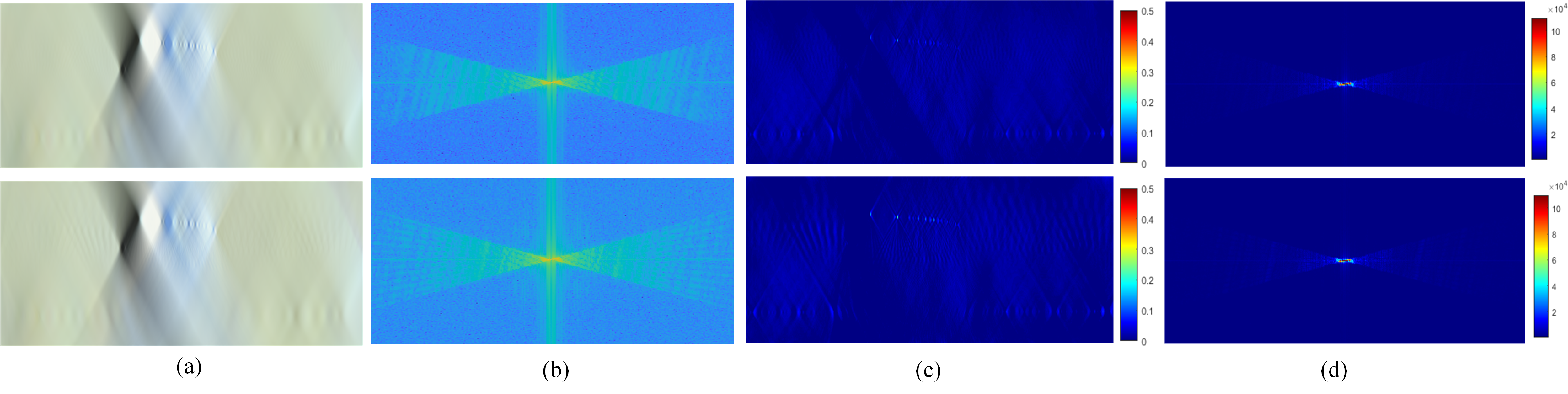
Figure 10: Reconstructed focal stack slices and FSS under different downsampling settings. Top: $5\times$ downsampling. Bottom: $15\times$ downsampling. (a) Anti-aliasing on the focal stack. (b) Reconstructed FSS. (c) Error map of the focal stack. (d) Error map of the FSS.

Figure 11: Aliasing-removed results at different focal layers under $5\times$ and $15\times$ downsampling rates. (a) Input image. (b) Ground truth. (c) Our result.

V-B Method Capacity

TABLE III: Average spectral energy loss on different test scenarios.

Dataset	$5\times$	$15\times$
Syn. LFs	2.03%	3.58%
Real LFs [31]	2.50%	3.13%
Lego [32]	0.56% ($2\times$)
Couch [33]	2.71% ($10\times$)
Church [33]	0.67% ($10\times$)

Figure 12: Quantitative results of our method across focal layers under different downsampling settings. Top: Tree scene. Bottom: Bicycle scene. (a) Absolute PSNR. (b) Relative PSNR. (c) Absolute SSIM. (d) Relative SSIM.

Spectrum Domain. In this subsection, we demonstrate the performance of our approach with respect to different sampling rates. Comparing Fig.3(b)(c) with Fig.10, we can see that, for different sampling rates, our method achieves a preferable performance on anti-aliasing rendering in both spatial and frequency domains. It is important to note that the errors in the frequency domain mainly come from the Direct Component (DC) of the spectrum. The main reason is that the energies of DC and its near neighborhoods are much larger than those of other components [27]. Also deep learning is more inclined to learn low-frequency components from an input signal map [36]. The differences will cause color defects during the FSS reconstruction stage. To tackle this problem, we replace the DC and its near neighborhoods ($5\times 5$ patch around the central pixel) of the output spectrum with those of the input spectrum. Tab. III shows the average spectral energy loss on different test scenarios. From Tab. III and Tab. V, it is found that the PSNR of our method is greatly affected by energy loss, while SSIM is little affected by it. According to [37], human visual system is more sensitive to the structural similarity than PSNR. Based on this assumption, the errors of defocus blur in refocused images are hard to detect by human eyes. Therefore a higher SSIM value in Tab. V demonstrates better performance of the proposed method.

Image Domain. Fig.11 shows the results of anti-aliasing in different focal images under $5\times$ and $15\times$ downsampling settings. For the $5\times$ downsampling setting, the proposed method could remove aliasing around severely occluded objects (trees in the top row). The middle and bottom rows show the anti-aliasing results at different focal layers for the same scene (Bicycle) when the focused depth is beyond and within the range for the scene depth respectively. Although the radius of defocus blur varies, the proposed method could simultaneously eliminate the aliasing effects (the middle row) and retains the sharp edges (the bottom row), which shows the PSF-continuity is well maintained by the proposed method. For the $15\times$ downsampling setting, although the aliasing is more severe due to the larger disparity, our method can still obtain satisfied aliasing-removed results.

Fig.12 shows the quantitative results of our method across focal layers under different downsampling settings. The relative PSNR is obtained by subtracting the PSNR of the input focal layer image from the absolute PSNR. The same operation holds for the relative SSIM. As shown in Fig.12(b)(d), both PSNR and SSIM fluctuate with refocusing depth. It is noticed that, the relative PSNR/SSIM curves are not smooth. We believe it is due to the Tree scene is composed of trees with complex occlusion (see rightmost column of Fig.9), which causes many jitters in the PSNR/SSIM curves of the input focal stacks. Also when there is mild aliasing in the refocused image, the promotion of PSNR and SSIM is less obvious (see the bottom row in Fig.11). However, the varying trends of PSNR/SSIM curves demonstrate our approach maintains the continuity of PSF in the focal stack.

Figure 13: Anti-aliasing results on the Lego Knights scene [32] along the directions of $y-v$. From top to bottom: refocused image at a certain depth, partial focal stack along the yellow solid line, and corresponding FSS. (a) Input with aliasing (the view number is $17\times 1$); (b) Anti-aliasing result.

Figure 14: Aliasing-removed results under $5\times$, $15\times$, $20\times$ and $25\times$ downsampling rates. (a) Ground truth. (b) Input. (c) Output.

Figure 15: Quantitative comparisons of anti-aliasing results in Fig.14.

Figure 16: Anti-aliasing results on Bicycle from the HCI datasets [38] when refocusing at $d=-0.75$. (a) Ground truth. (b) Input with aliasing (the number of views is $1\times 2$). Results by (c) Dayan et al. [10] and (d) our method.

Figure 17: Anti-aliasing results under $15\times$ downsampling (refocused images and error maps). (a) Input focal image and ground truth. Results by (b) our method, (c) Kalantari et al. [11], (d) Xiao et al. [4], (e) Wu et al. [12] and (f) Le Pendu et al. [22]. The left half shows synthetic LFs and the right half shows real LFs. Several local areas are zoomed in for better visualization.

Figure 18: Anti-aliasing results on the focal stack slice under $15\times$ downsampling. (a) Ground truth. (b) Input. Results by (c) our method, (d) Kalantari et al. [11], (e) Xiao et al. [4], (f) Wu et al. [12] and (g) Le Pendu et al. [22]. The red arrow locates one of the focus points. The upper half shows synthetic LFs and the lower half shows real LFs. Several local areas are zoomed in for better visualization.

TABLE IV: Average PSNR/SSIM using different loss functions.

Scene	w/o. ${loss}_{s}$	w. ${loss}_{s}$
Tree (Syn. LF)	34.97 / 0.880	35.92 / 0.912
Bicycle (Real LF) [31]	33.08 / 0.949	34.45 / 0.960

Conjugate symmetry loss. To verify the effectiveness of the conjugate symmetry loss, an ablation experiment is conducted. Tab. IV shows the average PSNR/SSIM over the whole focal stack under $15\times$ downsampling with or without the $loss_{s}$. It is noticed that both PSNR and SSIM are improved by applying the conjugate symmetry loss in the U-Net.

Vertical EPI. All the above experiments are carried out in the $x\!-\!u$ subspace. Fig.13 shows the aliasing-removed results in the $y\!-\!v$ subspace on the Stanford light fields [32], from which we find that our method is also effective in the $y\!-\!v$ subspace of a 4D light field.

Undersampled light fields To verify the effectiveness of our method on undersampled light fields, we also conduct relative experiment on the HCI datasets [34]. For the StillLife scene, the disparity between adjacent views is larger than $\pm 1$ pixel, which produces severe aliasing effects when refocusing. As shown in Fig.1, when refocusing on the red cloth in the background, the bees and wooden balls in the foreground will be severely aliased. Our method can eliminate the aliasing well, which verifies the generalization of the proposed deep anti-aliasing algorithm.

Bound analysis and minimal angular sampling. In order to analyse the robustness of our method, we conduct experiments under $5\times$, $15\times$, $20\times$ and $25\times$ downsampling settings on the real light field [31] respectively. As shown in Fig.14, the refocused depth is located at the foreground yellow step. For the $5\times$ and $15\times$ downsampling settings, the proposed method could completely remove the aliasing. For the $20\times$ downsampling, although our method still works, the quality of the anti-aliased image decreases slightly (refer to the quantitative analysis in Fig.15). For the $25\times$ downsampling, there exits significant unremoved aliasing in the red rectangle. Fig.15 shows quantitative comparisons (PSNR/SSIM/LPIPS) at different focal layers.

Moreover, we utilize a light field containing only $1\times 2$ views and compare our method with the approach proposed by Dayan et al. [10] to verify the effectiveness of our method on the minimal angular sampling light field. We select the 3rd and 6th horizontal views for refocusing on the Bicycle scene [38]. As shown in Fig. 16, our method not only remove the aliasing in the defocus area but also maintains the scene structure well, especially for the thin structures (see the blue rectangle in Fig.16).

TABLE V: Quantitative comparisons with SOTAs under different downsampling rates on both synthetic and real LFs.

		Syn. LFs		Real LFs [31]		Lego [32]	Couch [33]	Church [33]
		$5\times$	$15\times$	$5\times$	$15\times$	$2\times$	$10\times$	$10\times$
Kalantari [11]	PSNR$\uparrow$	34.12	28.65	32.72	32.14	38.14	31.54	35.26
	SSIM$\uparrow$	0.852	0.825	0.864	0.851	0.907	0.954	0.887
	LPIPS$\downarrow$	0.113	0.154	0.095	0.17	0.094	0.084	0.141
Xiao [4]	PSNR$\uparrow$	31.75	30.51	32.91	32.71	39.09	34.38	35.97
	SSIM$\uparrow$	0.903	0.844	0.907	0.872	0.939	0.964	0.937
	LPIPS$\downarrow$	0.108	0.179	0.085	0.130	0.097	0.086	0.147
Wu [12]	PSNR$\uparrow$	33.67	32.47	34.32	33.62	41.57	34.65	35.25
	SSIM$\uparrow$	0.926	0.887	0.957	0.946	0.945	0.933	0.881
	LPIPS$\downarrow$	0.106	0.146	0.084	0.112	0.042	0.066	0.115
Le Pendu [22]	PSNR$\uparrow$	34.20	32.41	33.69	32.78	39.16	34.99	35.28
	SSIM$\uparrow$	0.936	0.849	0.951	0.862	0.952	0.938	0.905
	LPIPS$\downarrow$	0.079	0.112	0.069	0.123	0.088	0.076	0.107
Ours	PSNR$\uparrow$	34.41	33.76	34.19	34.04	41.18	34.70	37.98
	SSIM$\uparrow$	0.952	0.923	0.962	0.956	0.962	0.961	0.951
	LPIPS$\downarrow$	0.072	0.097	0.046	0.064	0.052	0.065	0.094

V-C Comparison with SOTAs

Figure 19: Quantitative comparisons on two test scenes in Fig.17. The upper two rows are for synthetic LFs and the lower two rows are for real LFs.

In this subsection, we compare our method against 4 SOTAs, Kalantari et al. [11] , Xiao et al. [4], Wu et al. [12] and Le Pendu et al. [22]. Tab. V shows the average PSNR/SSIM/LPIPS on both synthetic (abbreviated in Syn.) and real light fields (Real for short) over all focal layers. Our proposed method achieves the best anti-aliasing performance for all scenes among all the methods. Qualitative comparisons on two test scenes are shown in Figs.17 and 18. Fig.19 shows the quantitative comparisons of Fig.17 at each focal layer.

Figure 20: Anti-aliasing results on the Disney datasets. (a) Ground truth. (b) Input focal image under $10\times$ downsampling. Results by (c) our method, (d) Kalantari et al. [11], (e) Xiao et al. [4], (f) Wu et al. [12], and (g) Le Pendu et al. [22]. Several local areas are zoomed in for better visualization.

Fig.17 compares the anti-aliasing results under $15\times$ downsampling. Our method outperforms all other methods. The method by Kalantari et al. [11] adopts a view synthesis network to eliminate the aliasing. However, this method does not perform well for view synthesis under large parallax. The object edges are distorted significantly. Extensive disparities and complex occlusions further lead to severe aliasing in the out-of-focus regions. For the second test scene, the focal plane is located on the yellow step ahead, so significant aliasing appears in the background. The method proposed by Wu et al. [12], which performs view synthesis via EPI interpolation, cannot deal with the light fields with large disparities and causes aliasing in the occlusion boundary areas and non-focus areas (as shown in the left half of Fig.17(e)). Although the method by Xiao et al. [4] can detect the aliasing area, it can not deal with the massive disparity situation. Moreover, to remove aliasing, this method increases the number of pyramid layers and then utilizes a multi-scale image fusion strategy to eliminate aliasing, however, the whole image will be consequently blurred (as shown in the left half of Fig.17(d)). The FDL model proposed by Le Pendu et al. [22] is prone to produce visible errors due to large occlusion areas or non-Lambertian effects, such as the occlusion and edge areas shown in the error map of Fig.17(f).

According to the analysis in Section III-B, the focal stack is PSF-continuous, i.e., the radius of defocus is linearly and smoothly changed along the $f$-axis and symmetrical with the focused depth layer. Maintaining this characteristic is one of the most important indicators for evaluating the anti-aliasing effects. Fig.18 shows the results with different focal parameters under the $15\times$ downsampling setting. View synthesis methods (Kalantari et al. [11], Wu et al. [12] and Le Pendu et al. [22]) could only provide non-aliasing results on certain focal layers with moderate defocus radii, and for the focal layers with large defocus radii these methods suffer a severe performance drop. Specifically, as shown in the red rectangles on synthetic scenes, obvious aliasing still exists in the results of view synthesis methods (Fig.18(d)(f)(g)). Also, the focused points could be over-smoothed (green rectangle and areas pointed by the red arrow on the synthetic scenes). Apart from this, previous anti-aliasing methods (e.g. Xiao et al. [4]) eliminate aliasing on different layers separately. This makes the radius of defocus no longer change linearly or smoothly, thus the PSF-continuity in the focal stack is broken. Specifically, we can observe discontinuous changes in the radius of defocus in the green rectangles on synthetic scenes (Fig.18(e)), also the sudden jumps along the yellow curve in Fig.19. On the contrary, the proposed method provides consistent anti-aliasing results and preserves the PSF-continuity in the focal stack.

Quantitative results are shown in Fig.19. We report quantitative performance using the standard PSNR and SSIM metrics (server uptime), as well as the state-of-the-art LPIPS [39] perceptual metric (server performance), which is based on a weighted combination of neural network activations tuned to match human judgements on image similarity. In most cases, our method outperforms the SOTAs, especially in the case of large parallax ($15\times$ downsampling). The PSNRs of Xiao et al. [4] are higher than those of our method on several focal layers, however, since Xiao et al. [4] process each refocused image separately and can not guarantee the continuity of the PSF, the overall trends of its PSNR, SSIM and LPIPS curves fluctuate along the sampling rate.

Results on light fields captured by a camera array. In order to verify the generalization of our algorithm, we test our method on the Disney datasets [33] and the Lego scene from the Stanford datasets [32]. Because the angular resolutions of these two LFs differ from other synthetic and real LFs (see Tab. III and V), we set the sampling rates for these two datasets as $10\times$ and $2\times$ respectively to guarantee the same angular resolution in the downsampling LFs (9 views). Fig.20 compares the anti-aliasing results on Church. When the image is refocused on the tree in front, there are obvious aliasing effects in the non-focusing areas. Comparing with SOTAs, our method can not only significantly remove the aliasing effects in the non-focusing areas, such as the white building in the distance (red rectangle) but also eliminate the aliasing near thin structures (green rectangle). The average PSNR, SSIM and LPIPS over the whole aliasing-removed focal stack are listed in the last three rows of Tab. V. Please refer to the supplementary video for more anti-aliasing results.

Figure 21: Focal stack slice and its FSS on Lego [32]. The focal stack and FSS are obtained using vertical-horizontal direction ($u,v$) views and horizontal direction ($u$) views only respectively. The top row shows the focal stack and the bottom displays the corresponding FSS. (a) The number of views is 9$\times$9 ($2\times$ downsampling). (b) The number of views is 1$\times$9 ($2\times$ downsampling).

V-D Discussion and Limitation

Currently, the proposed method could only process the light field with one angular dimension. For a 4D light field with two angular dimensions, the contents from different image rows break the linear structure (the cone-shaped pattern) in the focal stack (see red rectangle in Fig.21), which means the characteristics of the FSS are disabled.

To perform the anti-aliasing operation on a full 4D light field, we adopt a two-stage sequential strategy. As shown in Eqns.12 and 13, a 4D refocus operation could be decomposed into two 3D refocus operations in the horizontal and vertical 3D light field respectively.

$$\small I=\frac{1}{{{N_{v}}}}\sum\limits_{v}{\frac{1}{{{N_{u}}}}}\sum\limits_{u}{LF(u,v,x+ud,y+vd)}.$$ (12)

$$\begin{array}[]{l}L{F_{3D}}(v,x,y)=\frac{1}{{{N_{u}}}}\sum\limits_{u}{LF(u,v,x+ud,y)}\\ I=\frac{1}{{{N_{v}}}}\sum\limits_{v}{L{F_{3D}}}(v,x,y+vd)\end{array}.$$ (13)

Following Eqn.13, we first perform the horizontal aliasing-removing, and then the vertical aliasing-removing. Figs.22(c)-(f) show the anti-aliasing results on the Origami LF [38] where $d=1$. Figs.22(g)-(i) show quantitative results at different focal layers. Compared with existing methods (Xiao et al. [4], Wu et al. [12] and Le Pendu et al. [22]), the proposed method successfully removes the aliasing in the foreground and meanwhile keeps the focused areas unaffected.

However, there are still some limitations of the 4D solution. In terms of the results, since we remove the aliasing in the horizontal and vertical dimensions sequentially, accumulation errors are introduced and the PSNR/SSIM values decrease to a certain degree compared with the case on a 3D light field. In addition, anti-aliasing based on EPI can not guarantee the consistency from row-to-row well. In terms of applications, the two-stage sequential solution requires a structured view distribution (such as Fig.23(a)) and can not handle light fields with unstructured view distributions (such as Fig.23(b)).

Figure 22: Aliasing-removed results on the 4D Origami LF [38]. (a) Ground truth (the view count is $9\times 9$). (b) Input image (the number of views is $5\times 5$). (c) Our result. (d) PSNR. (e) SSIM. (f) LPIPS.

Figure 23: Schematic diagram of views distribution. (a) Structured arrangement. (b) Unstructured arrangement.

VI Conclusions and Future Work

In this paper, we propose an FSS-based deep anti-aliasing method for angularly undersampled light fields. The FSS representation preserves the PSF-continuity and spectrum distribution under different angular sampling rates. Since the depth cue is implicitly embedded in the FSS, the proposed anti-aliasing method only needs a rough depth range estimation instead of explicit depth estimations and can simultaneously enhance different refocused images along the focal direction. Experimental results show the effectiveness and robustness of the proposed method for challenging situations, such as large disparities and complex occlusions.

To better reveal the relation between the angular sampling rate and the FSS, for now, we mainly concern a 3D light field which contains either horizontal or vertical angular sampling. By simply extending the proposed method to a 4D light field (Sec.V-D), the accumulative errors are introduced and thus hinder the anti-aliasing results. In the future, we will focus on this issue and explore the FSS formed from a 4D light field.

Supplementary.pdf,1-2

References

- [1] A. Isaksen, L. McMillan, and S. J. Gortler, “Dynamically reparameterized light fields,” in ACM SIGGRAPH. ACM Press/Addison-Wesley Publishing Co., 2000, pp. 297–306.
- [2] R. Ng, “Digital light field photography,” Ph.D. dissertation, Stanford university, 2006.
- [3] J.-X. Chai, X. Tong, S.-C. Chan, and H.-Y. Shum, “Plenoptic sampling,” in ACM SIGGRAPH. ACM Press/Addison-Wesley Publishing Co., 2000, pp. 307–318.
- [4] Z. Xiao, Q. Wang, G. Zhou, and J. Yu, “Aliasing detection and reduction scheme on angularly undersampled light fields,” IEEE TIP, vol. 26, no. 5, pp. 2103–2115, 2017.
- [5] T. Georgiev and A. Lumsdaine, “Reducing plenoptic camera artifacts,” in Computer Graphics Forum, vol. 29, no. 6. Wiley Online Library, 2010, pp. 1955–1968.
- [6] M. Levoy and P. Hanrahan, “Light field rendering,” in ACM SIGGRAPH. ACM, 1996, pp. 31–42.
- [7] A.-C. Chang, T.-P. Sung, K.-T. Shih, and H. H. Chen, “Anti-aliasing for light field rendering,” in IEEE ICME. IEEE, 2014, pp. 1–6.
- [8] A. Lumsdaine, T. Georgiev et al., “Full resolution lightfield rendering,” Indiana University and Adobe Systems, Tech. Rep, vol. 91, p. 92, 2008.
- [9] D. G. Dansereau, O. Pizarro, and S. B. Williams, “Linear volumetric focus for light field cameras,” ACM TOG, vol. 34, no. 2, p. 15, 2015.
- [10] S. Ben Dayan, D. Mendlovic, and R. Giryes, “Deep sparse light field refocusing,” in BMVC. Springer, 2020.
- [11] N. K. Kalantari, T.-C. Wang, and R. Ramamoorthi, “Learning-based view synthesis for light field cameras,” ACM TOG, vol. 35, no. 6, pp. 193:1–193:10, 2016.
- [12] G. Wu, M. Zhao, L. Wang, Q. Dai, T. Chai, and Y. Liu, “Light field reconstruction using deep convolutional network on epi,” in IEEE CVPR, 2017, pp. 1638–1646.
- [13] H. Lin, C. Chen, S. B. Kang, and J. Yu, “Depth recovery from light field using focal stack symmetry,” in IEEE ICCV, 2015.
- [14] T. Broad and M. Grierson, “Light field completion using focal stack propagation,” in ACM SIGGRAPH 2016 Posters, 2016, pp. 1–2.
- [15] S. J. Gortler, R. Grzeszczuk, R. Szeliski, and M. F. Cohen, “The lumigraph,” in Proceedings of the 23rd annual conference on Computer graphics and interactive techniques, 1996, pp. 43–54.
- [16] R. Ng, “Fourier slice photography,” in ACM TOG, vol. 24, no. 3. ACM, 2005, pp. 735–744.
- [17] A. Levin, W. T. Freeman, and F. Durand, “Understanding camera trade-offs through a bayesian analysis of light field projections,” in Springer ECCV, 2008, pp. 88–101.
- [18] H. W. F. Yeung, J. Hou, J. Chen, Y. Y. Chung, and X. Chen, “Fast light field reconstruction with deep coarse-to-fine modelling of spatial-angular clues,” in Springer ECCV, 2018, pp. 137–152.
- [19] B. Mildenhall, P. P. Srinivasan, R. Ortiz-Cayon, N. K. Kalantari, R. Ramamoorthi, R. Ng, and A. Kar, “Local light field fusion: Practical view synthesis with prescriptive sampling guidelines,” TOG, vol. 38, no. 4, pp. 1–14, 2019.
- [20] P. P. Srinivasan, R. Tucker, J. T. Barron, R. Ramamoorthi, R. Ng, and N. Snavely, “Pushing the boundaries of view extrapolation with multiplane images,” in IEEE CVPR, 2019, pp. 175–184.
- [21] T. E. Bishop and P. Favaro, “The light field camera: Extended depth of field, aliasing, and superresolution,” TPAMI, vol. 34, no. 5, pp. 972–986, 2011.
- [22] M. Le Pendu, C. Guillemot, and A. Smolic, “A fourier disparity layer representation for light fields,” IEEE TIP, vol. 28, no. 11, pp. 5740–5753, Nov 2019.
- [23] M. Le Pendu and A. Smolic, “High resolution light field recovery with fourier disparity layer completion, demosaicing, and super-resolution,” in 2020 IEEE International Conference on Computational Photography (ICCP). IEEE, 2020, pp. 1–12.
- [24] L. Shi, H. Hassanieh, A. Davis, D. Katabi, and F. Durand, “Light field reconstruction using sparsity in the continuous fourier domain,” ACM TOG, vol. 34, no. 1, pp. 12:1–12:13, 2014.
- [25] S. Vagharshakyan, R. Bregovic, and A. Gotchev, “Light field reconstruction using shearlet transform,” IEEE T-PAMI, vol. 40, no. 1, pp. 133–147, 2018.
- [26] J. Bigun and G. H. Granlund, “Optimal orientation detection of linear symmetry,” in IEEE ICCV, 1987, pp. 433–438.
- [27] R. C. Gonzales and R. E. Woods, “Digital image processing,” 2002.
- [28] O. Ronneberger, P. Fischer, and T. Brox, “U-net: Convolutional networks for biomedical image segmentation,” in International Conference on Medical image computing and computer-assisted intervention. Springer, 2015, pp. 234–241.
- [29] H. Zhu, M. Guo, H. Li, Q. Wang, and A. Robles-Kelly, “Revisiting spatio-angular trade-off in light field cameras and extended applications in super-resolution,” IEEE TVCG, pp. 1–1, 2019.
- [30] POV-ray, http://www.povray.org/.
- [31] M. Guo, H. Zhu, G. Zhou, and Q. Wang, “Dense light field reconstruction from sparse sampling using residual network,” in Springer ACCV, 2018, pp. 1–14.
- [32] “The new stanford light field archive,” http://lightfield.stanford.edu/lfs.html.
- [33] C. Kim, H. Zimmer, Y. Pritch, A. Sorkine-Hornung, and M. H. Gross, “Scene reconstruction from high spatio-angular resolution light fields,” ACM TOG, vol. 32, no. 4, pp. 73:1–73:12, 2013.
- [34] K. Honauer, O. Johannsen, D. Kondermann, and B. Goldluecke, “4D light field dataset,” https://www.cvia.uni-konstanz.de/code-and-datasets/, 2016.
- [35] D. P. Kingma and J. Ba, “Adam: A method for stochastic optimization,” in ICLR, 2015.
- [36] N. Rahaman, A. Baratin, D. Arpit, F. Draxler, M. Lin, F. Hamprecht, Y. Bengio, and A. Courville, “On the spectral bias of neural networks,” in ICML. PMLR, 2019, pp. 5301–5310.
- [37] Z Wang, A. C. Bovik, H. R. Sheikh, and E. P. Simoncelli, “Image quality assessment: from error visibility to structural similarity,” IEEE TIP, vol. 13, no. 4, pp. 600–612, 2004.
- [38] K. Honauer, O. Johannsen, D. Kondermann, and B. Goldluecke, “A dataset and evaluation methodology for depth estimation on 4d light fields,” in Asian Conference on Computer Vision. Springer, 2016, pp. 19–34.
- [39] R. Zhang, P. Isola, A. A. Efros, E. Shechtman, and O. Wang, “The unreasonable effectiveness of deep features as a perceptual metric,” in IEEE CVPR, 2018, pp. 586–595.