Oscillation time and damping coefficients in a nonlinear pendulum

Abstract

We establish a relationship between the normalized damping coefficients and the time that takes a nonlinear pendulum to complete one oscillation starting from an initial position with vanishing velocity. We establish some conditions on the nonlinear restitution force so that this oscillation time does not depend monotonically on the viscosity damping coefficient.

ASC2020: 34C15, 34C25

Keywords. oscillation time, damping, damped oscillations

This paper is dedicated to the memory of Prof. Alan Lazer (1938-2020), University of Miami. It was my pleasure to discuss with him some of the results presented here

1 Introduction

The pendulum is perhaps the oldest and fruitful paradigm for the study of an oscillating system. The apparent regularity of an oscillating mass going to and fro through the equilibrium position has fascinated the scientists well before Galileo. There are plenty of mathematical models accounting for almost any observed behavior of the pendulum’s oscillation. From the sheer amount of the literature on the subject, one would expect that there is no reasonable question regarding a pendulum that has no been already answered. And that might be true. Yet, for whatever reason, it is not impossible to take on a question whose answer does not seem to follow immediately from the classical sources.

In a typical experimental setup with no noticeable damping, the oscillations of a pendulum are periodic. Now, if the damping cannot be neglected, we still observe oscillations, even though they are non periodic. However, we can measure the time spent by a complete oscillation, and this time is a natural generalization of the period. But, how does depend this oscillation time on the characteristic of the medium, say on the viscosity of the surrounding atmosphere? It seems that there is no much information on how the damping affects the oscillation time. There are plenty of new publications regarding damping and oscillations, ranging from analytical solutions ([5], [3],[6]), to very clever experimental setups (see for example [4]). The nature of the damping has been also extensively considered ([8], [2]), but the dependence of the oscillation time on the damping or on the non-linearity seems to be less investigated.

For the sake of simplicity we analyze the oscillation time in the frame of a model that appear in almost any text book of ordinary differential equations (see for example [1]):

$$\ddot{x}+2\alpha\,\dot{x}+x\left(1+f\left(x\right)\right)=0,$$ (1)

where $x=x(t)$ measures the pendulum’s deviation with respect to a vertical axis of equilibrium and $\alpha\geq 0$ denote the viscous damping coefficient. The term $x\,f(x)$ models the nonlinear part of the restoring force. We’ve rescaled the time so that the period of the linear undamped oscillation is exactly $2\pi$.

The math of the solutions $x=x(t)$ is classical. If $f$ is smooth and $x_{0}$ and $v_{0}$ are given real values, then there exists a unique solution satisfying the given conditions $x(0)=x_{0}$ and $\dot{x}(0)=v_{0}.$ Moreover, if $f(0)=0$, then $x=0$ is a stable equilibrium solution of (1). As a consequence, $x(t)$ is defined for all $t\geq 0$ provided $|x_{0}|\ll 1$ and $|v_{0}|\ll 1$. Notice that the points of vanishing derivative of a solution $x=x(t)$ to (1) are isolated and those points correspond, either to local maxima or to local minima. Denote by $\tau(x_{0},\alpha)$ the amount of time spent (by the mass) completing one oscillation starting from $x_{0}$ with vanishing velocity ($v_{0}=0$). To be precise, if $x=x(t)$ starts from $x_{0}$ with vanishing velocity, then $x$ reaches a local maximum at $t=0$, and the oscillation is completed when $x$ reaches the next local maximum. Certainly, the oscillation time generalizes the period of solutions for the undamped model ($\alpha=0$). In this investigation we analyze the dependence of $\tau$ on $x_{0}$ and on $\alpha$ under the following working hypothesis:

Assumption 1.1.

On small $\epsilon-$neighborhood of $0$ the function $f$ is even and for some constant $a>0$ we have

$$f(x)=-a\,x^{2}+O\left(|x|^{4}\right),$$

We shall show that for $x_{0}$ fixed, $\tau$ reaches a positive minimum at some $0<\alpha_{0}<1.$ It does not seem obvious that an increase in the damping coefficient $\alpha$ might cause a decrease in $\tau$. It is also worth noticing that the existence of a minimum of $\tau$ is a consequence the sign of the constant $a$ in the above assumption. Indeed, according to numerical experiments carried out by the author, $\tau$ does not reach a positive minimum if $a<0$. The author is not aware of a similar result in the current literature nor whether this phenomena has been experimentally addressed. The whole paper was written with the aim at the mathematical pendulum $x(1+f(x))=\sin{x}.$ In that case, Figure 1 summarize our findings by picturing the numerically simulated value for $\tau(x_{0},\alpha)$. Interestingly, our qualitative analysis accurately reflects variations of $\tau$ that are not easy to spot numerically. For instance, the minimum of $\tau(x_{0},\alpha)$ for $x_{0}=0.1$ is not evident in Figure 1.

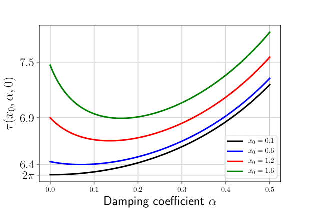
Figure 1: Numerical simulation $\tau(x_{0},\alpha)$ depending on $\alpha$ for several values of $x_{0}$. The nonlinear term $f$ was chosen so that $x(1+f(x))=\sin{x}.$

The arguments and proofs in this paper are entirely based on well established techniques of ODE theory. However, the main result (Theorem 3.1) rests on delicate estimates involving a differential equation describing the dependence of the solution $x=x(t)$ with respect to $\alpha$.

2 Underdamped oscillations

Definitions of underdamped oscillations in linear systems naturally carry over to solutions of (1). From now on, $x(\cdot,x_{0},\alpha)$ stands for the unique solution to (1) satisfying the initial condition $x(0)=x_{0}$ and $\dot{x}(0)=0.$ We also write $\tau(x_{0},\alpha)$ to highlight the dependence of the oscillation time on $x_{0}$ and $\alpha$. We will write simply $\tau$ or $x$ when no confusion can arise. It is convenient to represent (1) in the phase space $(x,v)$ with $\dot{x}=v:$

$$\begin{split}\dot{x}&=v\\ \dot{v}&=-2\alpha\,v-x-x\,f\left(x\right).\\ \end{split}$$ (2)

Equation (2) is explicitly solvable whenever $f\equiv 0$, and in that case, its solution is given by

$$\begin{split}x_{l}(t)=&\frac{e^{-\alpha\,t}}{\omega}\left(\omega\,\cos{\omega\,t}+\alpha\,\sin{\omega\,t}\right)x_{0}\\ v_{l}(t)=&-\frac{e^{-\alpha\,t}}{\omega}\,\sin{\omega\,t}\,x_{0}\end{split}$$ (3)

where $\omega=\sqrt{1-\alpha^{2}}$. Moreover, the oscillation time $\tau_{l}$ is given by

$$\tau_{l}=\frac{2\pi}{\omega}=\frac{2\pi}{\sqrt{1-\alpha^{2}}}.$$

Notice that $\tau_{l}$ is an increasing function that solely depends on $\alpha$.

Though a closed-form solution of (1) is either not known or impractical, we could express the relevant solutions implicitly. To that end, we rewrite (2) so that the nonlinear term $-x\,f\left(x\right)$ assumes the role of a non homogeneous forcing term. The expression for the solution $(x,v)$ is implicitly given by

$$\begin{split}x(t)=&x_{l}(t)-\frac{1}{\omega}\int_{0}^{t}e^{-\alpha\left(t-s\right)}\sin\omega\left(t-s\right)x(s)\,f(x(s))\,ds\\ v(t)=&v_{l}(t)-\frac{1}{\omega}\int_{0}^{t}e^{-\alpha\left(t-s\right)}\left(\omega\,\cos{\omega\left(t-s\right)}-\alpha\sin\omega\left(t-s\right)\right)x(s)\,f(x(s))\,ds\end{split}$$ (4)

Next, we estimate the solutions of (2) in the conservative case ($\alpha=0$) in which all solutions are periodic and the period is given by $\tau\equiv\tau(x_{0},0).$

Lemma 2.1.

If $(x,v)$ stands for the solution to (2) with $\alpha=0$ that satisfies $(x(0),v(0))=(x_{0},0)$, then there exists $\delta>0$ so that for all $|x_{0}|\leq\delta$ and all $0\leq t\leq\tau$ we have

$$x(t)=x_{0}\,\cos t+R_{1}(t,x_{0}),\quad v(t)=-x_{0}\,\sin t+R_{2}(t,x_{0}),$$ (5)

where

$$|R_{i}(t,x_{0})|\leq\text{const }\,|x_{0}^{3}|,\quad i=1,2.$$

Proof.

Letting $\alpha=0$ in (4) we obtain

$$R_{1}(t,x_{0})=-\int_{0}^{t}\cos(t-s)\,x(s)\,f(x(s))\,ds.$$ (6)

Since $(0,0)$ is a stable equilibrium solution to (2), there exists $\delta>0$ and $\epsilon>0$ so that any solution $(x,v)$ to (2) starting at $(x_{0},0)$, with $|x_{0}|\leq\delta$ satisfies $|x(t)|\leq\epsilon$. Now write $F(z)=-z\,f(z)$ and notice that for some $\xi\in(-\epsilon,\epsilon)$ we have

$$F(x(s))=F\left(x_{0}\cos{s}+R_{1}\left(s,x_{0}\right)\right)=F\left(x_{0}\cos{s}\right)+R_{1}\left(s,x_{0}\right)F^{\prime}\left(\xi\right).$$

Next, identity (6), Assumption (1.1) and some standard estimations yield

$$|R_{1}(t,x_{0})|\leq 2a|x_{0}^{3}|+c_{2}\int_{0}^{t}|R_{1}(s,x_{0})|\,ds$$

where $c_{2}=\max_{z\in[-\epsilon,\epsilon]}|F^{\prime}(z)|$. The first claim follows now from Gronwall’s inequality. The proof of the estimation for $R_{2}$ is analogous. ∎

At this point it is appropriated to define the half oscillation time $\hat{\tau}=\hat{\tau}(x_{0},\alpha)$ to be the time spent by the solution $x(t,x_{0},\alpha),$ $t\geq 0,$ reaching the next local minimum. If $\alpha=0$ and $f$ is even, the symmetry of the solution (1) yields. $2\hat{\tau}=\tau.$

Lemma 2.2.

If $\hat{\tau}=\hat{\tau}(x_{0},\alpha)$ denote the half oscillation time and $a$ is the constant of Assumption 1.1, then

$$\hat{\tau}(x_{0},\alpha)>\frac{\pi}{\sqrt{1-\alpha^{2}}}\quad\text{and}\quad\lim_{x_{0}\to 0^{+}}\hat{\tau}(x_{0},0)=\pi+\frac{a\,\pi}{8}\,x_{0}^{2}+o(x_{0}^{3}).$$

Proof.

We introduce introduce the polar coordinates

$$r=\sqrt{x^{2}+v^{2}},\quad\tan{\theta}=\frac{x}{v},$$

to obtain

$$\begin{split}\dot{\theta}&=-\left(1+\alpha\,\sin{2\theta}+\sin^{2}{\theta}\,f\left(x\right)\right)\\ \dot{r}&=-\frac{v}{r}\left(2\alpha\,v+x\,f\left(x\right)\right)\\ \end{split}$$ (7)

As a consequence of equation (7) we obtain the following expression for the half oscillation time $\hat{\tau}=\hat{\tau}(x_{0},\alpha)$

$$\hat{\tau}=\int_{0}^{\pi}\frac{d\theta}{1+\alpha\,\sin{2\theta}+\sin^{2}{\theta}\,f\left(x(\theta)\right)}.$$ (8)

Now, the effect of the nonlinearity on the oscillation time is clear. By Assumption 1.1 we obtain

$$\hat{\tau}(x_{0},\alpha)>\int_{0}^{\pi}\frac{d\theta}{1+\alpha\,\sin{2\theta}}=\frac{\pi}{\sqrt{1-\alpha^{2}}}.$$

For $\alpha=0$ we use estimation (5) to obtain

$$\hat{\tau}(x_{0},0)=\int_{0}^{\pi}\frac{d\theta}{1-a\,x_{0}^{2}\,\sin^{2}{\theta}\,\cos^{2}{t(\theta)}}+o(x_{0}^{3}).$$

Now a straightforwards computation yields

$$\lim_{x_{0}\to 0^{+}}\hat{\tau}(x_{0},0)=\pi,\;\lim_{x_{0}\to 0^{+}}\frac{\partial\hat{\tau}}{\partial x_{0}}(x_{0},0)=0.$$

Now, the expression for $\frac{\partial^{2}\hat{\tau}}{\partial x_{0}^{2}}(x_{0},0)$ is somewhat cumbersome. However, taking into account that $\lim_{x_{0}\to 0}t(\theta)=\theta$, we readily obtain

$$\lim_{x_{0}\to 0^{+}}\frac{\partial^{2}\hat{\tau}}{\partial x_{0}^{2}}(x_{0},0)=\int_{0}^{\pi}2a\,\sin^{2}{\theta}\,\cos^{2}{\theta}\,d\theta=\frac{2\,a\pi}{8},$$

and the second claim of the lemma follows by the second order Taylor expansion of $\hat{\tau}(x_{0},0)$ around $x_{0}$ ∎

A reasoning analogous to that in the proof of the preceding lemma shows that

$$\tau(x_{0},\alpha)>\frac{2\pi}{\sqrt{1-\alpha^{2}}}\equiv\tau_{l}.$$

This inequality is illustrated in Figure 2 when $a=1$. Had we considered in Assumption 1.1 negative values for $a$, then the inequality would reverse to $\tau(x_{0},\alpha)<\tau_{l}$ as it is depicted in Figure 2.

3 The role of the viscous damping

It is not difficult at all to obtain a differential equation describing the movement of the pendulum depending on the viscous damping coefficient. Indeed, writing

$$X(t,x_{0},\alpha)=\frac{\partial x}{\partial\alpha}\left(t,x_{0},\alpha\right),\quad V(t,x_{0},\alpha)=\frac{\partial v}{\partial\alpha}\left(t,x_{0},\alpha\right).$$

Derivation of equation (2) with respect to $\alpha$ yields:

$$\begin{split}\dot{X}&=V\\ \dot{V}&=-2\alpha\,V-X-2v-\left(x\,f^{\prime}\left(x\right)+f\left(x\right)\right)X.\end{split}$$ (9)

As for the initial conditions we have

$$X(0,x_{0},\alpha)=0,\quad V(0,x_{0},\alpha)=0.$$

Let us write $G(x)=-\frac{d}{dx}\left(x\,f\left(x\right)\right)$. Again, as we did with equation (2), equation (9) can be seen as a linear homogeneous part plus the forcing term $-2v+G(x)\,X.$ The solution $X,V$ is implicitly given by

$$\begin{split}X(t)=&\frac{1}{\omega}\int_{0}^{t}e^{-\alpha\left(t-s\right)}\sin\omega\left(t-s\right)\big{\{}\\ &\qquad-2v(s)+G(x(s))\,X(s)\left.\right\}ds\\ V(t)=&\frac{1}{\omega}\int_{0}^{t}e^{-\alpha\left(t-s\right)}\left(\omega\,\cos{\omega\left(t-s\right)}-\alpha\sin\omega\left(t-s\right)\right)\big{\{}\\ &\qquad-2v(s)+G(x(s))\,X(s)\left.\right\}ds\end{split}$$

In particular, for $\alpha=0$ the above expressions reduce to

$$\begin{split}X(t)=&\int_{0}^{t}\sin\left(t-s\right)\big{\{}-2v(s)+G(x(s))\,X(s)\big{\}}\,ds\\ V(t)=&\int_{0}^{t}\cos{\left(t-s\right)}\big{\{}-2v(s)+G(x(s))\,X(s)\big{\}}\,ds\end{split}$$ (10)

The following lemma does the heavy lifting to deliver the main result of the paper.

Lemma 3.1.

Under Assumption 1.1, if $\hat{\tau}=\hat{\tau}(x_{0},0)$ denotes the half oscillation time when $\alpha=0$, then for $0<x_{0}\ll 1$ we have $V(\hat{\tau},x_{0},0)>0.$

Proof.

We start with an auxiliary estimate for $X(t)$ in equation (10). By Lemma (2.1) and by Assumption 1.1, for $0<t\leq\pi$ we have

$$X(t)=x_{0}\left(-t\,\cos{t}+\sin{t}\right)+3a\,x_{0}^{2}\,\int_{0}^{t}\sin\left(t-s\right)\cos^{2}{s}\,X(s)\,ds+O(|x_{0}|^{4})$$ (11)

Notice that $X_{1}(t)\equiv x_{0}\left(-t\,\cos{t}+\sin{t}\right)$ does not vanish on $(0,\pi)$ and that $G(x(s))>0$ provided $0<x_{0}\ll 1$. Further, the initial conditions for $X(t)$ at $t=0$ and equation (9) yield that

$$X(0)=0=\dot{X}(0)=\ddot{X}(0)\text{ and }\dddot{X}(0)=2x_{0}\left(1+f\left(x_{0}\right)\right)>0,$$

meaning that $X(t)$ is positive on an interval $(0,\epsilon)$ with $\epsilon>0$. We claim that $X(t)>0$ for $0<t\leq\pi.$ On the contrary, there exists $\epsilon<t_{0}<\pi$ such that $X(t_{0})=0$ and $X(t)>0$ for $t\in(0,t_{0})$. Now, by Lemma 2.2 we know that $\hat{\tau}>\pi$. Therefore, the polar angle $\theta(t)$ in (7) satisfies $-\pi<\theta(t)<0$ for all $0<t<\pi$ and a fortiori $v(t)<0$ on $(0,\pi]$. But this is a contradiction to the first equation of (10) evaluated at $t=t_{0}$ since for $s\in(0,t_{0})$ we have

$$\sin\left(t_{0}-s\right)\big{\{}-2v(s)+G(x(s))\,X(s)\big{\}}>0.$$

Next, by the equation (11) it follows immediately that $X(t)=X_{1}(t)+O(|x_{0}|^{3})$. Analogously, for $V(t)$ we obtain

$$\begin{split}V(t)=&x_{0}\,t\,\sin{t}+3a\,x_{0}^{2}\int_{0}^{t}\cos\left(t-s\right)\cos^{2}{s}\,X_{1}(s)\,ds+O(|x_{0}|^{4})\\ \equiv&V_{1}(t)+V_{2}(t)+O(|x_{0}|^{4})\end{split}$$

where $V_{1}(t)\equiv x_{0}\,t\,\sin{t}$. Now, $V_{2}(t)$ can be explicitly evaluated. For the reader’s convenience, we write the complete expression for $V_{2}:$

$$\begin{split}V_{2}(t)=&3a\,x_{0}^{3}\Big{(}-\frac{1}{32}\,(6\,t^{2}+5)\,\cos{t}-\frac{3}{32}\,t\,\sin{3\,t}-\\ &\frac{1}{16}\,t\,\sin{t}-\frac{17}{128}\,\cos{3\,t}+\frac{37}{128}\,\cos{t}\Big{)}.\end{split}$$

Moreover, it is somewhat tedious but straightforward to show that $V_{2}$ is positive and increasing on a small neighborhood of $\pi$. By Lemma 2.2 $\hat{\tau}>\pi$, therefore

$$V_{2}(\hat{\tau})>V_{2}(\pi)=\frac{9a\,x_{0}^{3}\,\pi^{2}}{16}.$$

Again, by Lemma 2.2 we obtain

$$\begin{split}V_{1}(\hat{\tau})=&V_{1}(\pi)+\left(\hat{\tau}-\pi\right)V_{1}^{\prime}(\pi)+O(|x_{0}|^{4})\\ =&-\frac{a\,x_{0}^{3}\,\pi^{2}}{8}+O(|x_{0}|^{4}),\end{split}$$

so that $V(\hat{\tau})=V_{1}(\hat{\tau})+V_{2}(\hat{\tau})>0.$ ∎

Now we are in a position to show the main result of the paper

Theorem 3.1.

Under Assumption 1.1, there exists a $\delta>0$ such that for $0<x_{0}<\delta$ fixed, the oscillation time $\tau(x_{0},\alpha)$, for $0<\alpha<1$, reaches a positive minimum at some $0<\alpha<1$. Moreover,

$$\lim_{\alpha\to 1^{-}}\tau(x_{0},\alpha)=\infty.$$

Proof.

We let $0<x_{0}\ll 1$ fixed by now and denote by $(x,v)$ be the solution of equation (2). By definition of $\hat{\tau}$ we have $v(\hat{\tau},\alpha)=0$, so that the Implicit Function Theorem yields

$$\frac{\partial\hat{\tau}}{\partial\alpha}\,\dot{v}(\hat{\tau},\alpha)+V(\hat{\tau},\alpha)=0,$$

therefore

$$\frac{\partial\hat{\tau}}{\partial\alpha}=\frac{V(\hat{\tau},\alpha)}{x\left(\hat{\tau},\alpha\right)\left(1+f\left(x\left(\hat{\tau},\alpha\right)\right)\right)}.$$

Since $x\left(\hat{\tau},\alpha\right)$ is negative, it follows from Lemma 3.1 that and $\frac{\partial\hat{\tau}}{\partial\alpha}|_{\alpha=0}<0$. Now we shall show that the last inequality holds for the oscillation time $\tau$. To do that, write $\hat{x}_{0}=-x(\hat{\tau}(\alpha,x_{0}),x_{0})$ and see that

$$\tau(\alpha,x_{0})=\hat{\tau}(\alpha,x_{0})+\hat{\tau}(\alpha,\hat{x}_{0}).$$

That is to say, the half oscillation time depends on $|x_{0}|$ only. Notice that $\hat{x}_{0}\leq x_{0}$ and the equality holds in the conservative case $\alpha=0$ only. Therefore

$$\frac{\partial\tau}{\partial\alpha}(\alpha,x_{0})=\frac{\partial\hat{\tau}}{\partial\alpha}(\alpha,x_{0})+\frac{\partial\hat{\tau}}{\partial\alpha}(\alpha,\hat{x}_{0})-\frac{\partial\hat{x}_{0}}{\partial\alpha}(\alpha,x_{0})\,\frac{\partial\hat{\tau}}{\partial\alpha}(\alpha,x_{0})=0.$$

Moreover, since

$$\frac{\partial\hat{x}_{0}}{\partial\alpha}(\alpha,x_{0})=v(\hat{\tau}(\alpha,x_{0}),x_{0})=0,$$

we have that

$$\lim_{x_{0}\to 0^{+}}\frac{\partial\tau}{\partial\alpha}(\alpha,x_{0})=2\lim_{x_{0}\to 0^{+}}\frac{\partial\hat{x}_{0}}{\partial\alpha}(\alpha,x_{0})$$

Finally, by the first claim of Lemma 2.2, $\tau(\alpha,x_{0})$ must attain a minimum at some $0<\alpha<1$. ∎

4 Conclusions and final remarks

An oscillating mass exhibits gradually diminishing amplitude in the presence of damping. The time spent by the mass completing one oscillation depends on several factors, as the model for the restoring force, how the oscillation starts, and the nature of the damping. For the sake of our discussion we consider a vertical pendulum with a nonlinear restoring force resembling the mathematical pendulum, letting the oscillation start at a small amplitude with vanishing velocity and a viscous damping model with a (normalized) viscosity coefficient $\alpha$. We have proved that the oscillation time $\tau\equiv\tau(\alpha)$ does not depend monotonically on $\alpha$, meaning that there exists a threshold $\alpha_{0}$ (which depends on the starting amplitude of the oscillation) such that $\tau$ reaches a local minimum at $\alpha_{0}$ (see Figure 1). It is worth noticing that this behavior cannot be observed if the restitution force is linear, i. e., what we report in this paper is essentially a nonlinear phenomenon.

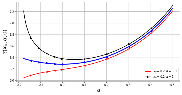
Figure 2: Numerical simulation of the oscillation time $\tau$ depending on the damping coefficient $\alpha$ with starting amplitude $x_{0}=0.2$ and non linear restoring term given by $f(x)=-a\,x^{2}$, $a=\pm 1$. The curve with the round marker (blue in the online version) corresponds to the oscillation time $\tau_{l}$ of the linear case $f\equiv 0$

The proof of existence of a positive minimum for the oscillation time rests heavily on the fact that the constant $a$ in Assumption 1.1 is positive. Just to experiment the effect of changing the sign of the constant $a$, we carried out some numerical simulations of $\tau$ with the nonlinear term $f(x)=-a\,x^{2}$ for $a=1,-1$. The corresponding equations are particular cases of an unforced Duffing oscillator [7]. The numerical results are shown in Figure 2. Just for the sake of the numerical experimentation we also considered negative values for $\alpha$. If $a=1$ we see that $\tau$ reaches its minimum at a positive value for $\alpha$. By contrast, if $a=-1$ no minimum seems to exist. The curve with the round marker (blue in the online version) corresponds to the oscillation time of the linear case $\tau_{l}=\frac{2\pi}{\sqrt{1-\alpha^{2}}}$.

The numerical experimentation of the oscillation time $\tau$ (not shown in this paper) assuming a quadratic damping exhibits the same behavior as the graphics of Figure 2. If the readers are curious about the numerical experiments, they could take a look at the author’s GitHub page

https://github.com/arangogithub/Oscillation-time

and download a Jupyter notebook with the python code featuring the results shown in Figures 1 and 2

References

- [1] V. I. Arnold. Mathematical Methods of Classical Mechanics. Springer, 1989.
- [2] L. Cveticanin. Oscillator with strong quadratic damping force. Publ. Inst. Math. (Beograd) (N.S.), 85(99):119–130, March 2009.
- [3] A Ghose-Choudhury and Partha Guha. An analytic technique for the solutions of nonlinear oscillators with damping using the abel equation arxiv:1608.02324 [nlin.si], 2016.
- [4] Remigio Cabrera-Trujillo Niels C Giesselmann Dag Hanstorp Javier Tello Marmolejo, Oscar Isaksson. A fully manipulable damped driven harmonic oscillator using optical levitation. American Journal of Physics, 88(6):490–498, sep 2018.
- [5] Kim Johannessen. An analytical solution to the equation of motion for the damped nonlinear pendulum. European Journal of Physics, 35(3):035014, mar 2014.
- [6] D Kharkongor and Mangal C Mahato. Resonance oscillation of a damped driven simple pendulum. European Journal of Physics, 39(6):065002, sep 2018.
- [7] S. Wiggins. Introduction to Applied Nonlinear Dynamical Systems and Chaos. Springer, 1990.
- [8] L F C Zonetti, A S S Camargo, J Sartori, D F de Sousa, and L A O Nunes. A demonstration of dry and viscous damping of an oscillating pendulum. European Journal of Physics, 20(2):85–88, jan 1999.