The HI-halo mass relation at redshift $z\sim 1$ from the Minkowski functionals of 21 cm intensity maps

Abstract

The mean and the scatter of the HI content of a dark-matter halo as a function of the halo mass are useful statistics that can be used to test models of structure and galaxy formation. We investigate the possibility of constraining this HI-halo mass relation (HIHMR) from intensity maps of the redshifted 21 cm line. In particular, we use the geometry and topology of the brightness-temperature isocontours in a single frequency channel as quantified by the Minkowski functionals. First, we generate mock maps from a large N-body simulation considering the impact of thermal noise and foreground removal. We then use the Fisher information formalism to forecast constraints on a parametric model for the HIHMR. We consider a 20,000 deg² survey (originally proposed for dark-energy science) conducted with the Square Kilometre Array Phase 1 (SKA-1) MID observatory operating in single-dish mode. For a channel bandwidth of 2 MHz, we show that an integration time of a few$\,\times\,10^{4}$ s per pointing is sufficient to image the smoothed HI distribution at redshift $z\simeq 1$ and to measure the HIHMR in a nearly optimal way from the Minkowski functionals. Tighter constraints on some of the parameters can be obtained by using also an independent measurement of the mean HI density. Combining the results from different frequency channels provides exquisite constraints on the evolution of the HIHMR, especially in the central frequency range of the data cube.

1 Introduction

Cold-gas reservoirs in galaxies provide the raw fuel for star formation. Assessing how they vary across different galaxy populations and environments is of paramount importance to constrain models of galaxy assembly and evolution.

Neutral hydrogen (HI) makes up the bulk of the cold gas. In the post-reionisation Universe, HI can be found almost exclusively within self-shielded clouds inside galaxies and galaxy clusters. The total HI content of dark-matter (DM) haloes is thus a simple descriptive statistic that can be used to compare theoretical models with observations. It gives the HI mass in a halo by summing up the contributions from central and satellite galaxies (as well as from diffuse gas). A strong theoretical prejudice is that this quantity should mainly depend on the halo mass. In fact, gas-accretion rates (both from the intergalactic medium and via galaxy mergers) are expected to be regulated by the halo masses and so are also several processes that deplete the HI content (like the efficiency of galactic winds or photoionisation). Extra dependencies on top of the halo mass will appear as scatter around the mean relation. Measuring the amplitude of this scatter provides an empirical test of the assumption that halo mass is the main driver of the HI content.

The HI-halo mass relation (HIHMR) has been the subject of many studies based on (post-processed) hydrodynamical simulations (Davé et al., 2013; Villaescusa-Navarro et al., 2014; Crain et al., 2017; Villaescusa-Navarro et al., 2018; Ando et al., 2019) and semi-analytical models of galaxy formation (Kim et al., 2017; Zoldan et al., 2017; Baugh et al., 2019; Spinelli et al., 2020). In parallel, observational constraints at redshift $2.2\lesssim z\lesssim 5$ have been obtained for damped Lyman-$\alpha$ absorbers (Barnes & Haehnelt, 2014). On the other hand, in the local Universe, extensive investigations have been carried out to elucidate the HIHMR of HI-rich galaxies from the Arecibo Fast Legacy ALFA Survey (ALFALFA, Giovanelli et al., 2005). For instance, Paul et al. (2018) have predicted the HIHMR by assuming that there exists a scaling relation between the HI content and the optical properties of a galaxy. By cross matching the ALFALFA HI sources with the optical group catalog from the Sloan Digital Sky Survey, Ai & Zhu (2018) have estimated the total HI mass for rich galaxy groups containing eight members or more. Combining a similar technique with information about the HI-weighed clustering of the ALFALFA sources, Obuljen et al. (2019) have constrained the parameters of an analytical model for the HIHMR. A direct measurement of the relation has been recently performed by Guo et al. (2020) who stacked the ALFALFA spectra of the members of the SDSS groups.

At intermediate redshifts ($0.1\lesssim z\lesssim 2.2$), we have very little information on the HI content of DM haloes as the 21 cm line is too faint to observe individual galaxies with reasonable integration times. A way out is to detect the collective emission from galaxies that occupy large ‘voxels’ in our past-light cone defined by the angular resolution and the bandwidth of the observations (21 cm tomography). The principal challenge for these intensity-mapping experiments is the subtraction of Galactic and extra-galactic foregrounds that are orders of magnitude brighter than the 21 cm signal. In order to filter them out, their properties and the instrumental systematics need to be characterized to extremely precise levels.

There is increasing interest in developing large-scale surveys that map the intensity of the 21 cm emission from neutral hydrogen to probe unprecedented volumes. Such experiments are expected to provide pivotal contributions to cosmology (e.g. Barkana & Loeb, 2005; Loeb & Wyithe, 2008; Monsalve et al., 2019) and, at higher redshifts, to our understanding of the epoch of reionisation (e.g. Yue & Ferrara, 2019).

Information about the HIHMR is key for predicting the signal of 21 cm intensity-mapping experiments. In full analogy with the halo model for dark-matter (e.g. Cooray & Sheth, 2002) and galaxy clustering (e.g. Scoccimarro et al., 2001), the HI distribution on large scales can be described in terms of its halo-occupation properties. By using the halo model to fit a compilation of data at low and high redshift, Padmanabhan et al. (2015) have estimated that the amplitude of the intensity-mapping signal at intermediate redshifts is between 50 and 100 per cent uncertain. Switzer et al. (2013) have obtained the first observational constraint on the amplitude of 21 cm fluctuations at $z\simeq 0.8$. There are some difficulties, however, in fitting this result together with the low-redshift studies and the Damped Lyman-$\alpha$ systems (DLAs) data into a consistent picture (Padmanabhan & Refregier, 2017; Padmanabhan et al., 2017).

In this work, we take the opposite step and investigate the possibility of inferring the HIHMR from the 21 cm intensity maps. However, in order not to weaken the constraining power of these experiments for cosmology, we do not use the power spectrum and focus on the geometrical and topological properties of the highly non-Gaussian maps as quantified by the Minkowski functionals (MFs) of their isocontours. Several morphological indicators have been already discussed in the 21 cm literature to characterise the growth of HII bubbles during the epoch of reionisation, namely, the genus curve (Hong et al., 2010), the MFs (Gleser et al., 2006; Chen et al., 2019), and the Minkowski tensor (Kapahtia et al., 2018). Here, we apply one of these methods to the post-reionisation Universe in order to constrain a parametric model for the HIHMR (mean and scatter). We use mock data based on a large N-body simulation and the Fisher information matrix to derive the constraints on the model parameters. The rationale behind our method is rather simple: since DM haloes of different masses trace the underlying mass-density distribution differently, the detailed morphology of the brightness-temperature maps should reflect the HIHMR.

We analyse here two-dimensional maps corresponding to individual frequency channels in a tomographic data cube. The main reason for this choice is that we can robustly estimate the covariance matrix of the data without having to run hundreds of high-resolution N-body simulations. Our method, however, can be straightforwardly generalised to three-dimensions by directly measuring the MFs in the full data cube.

The proposed approach requires rather long radio integration times as it is necessary to image the redshifted 21 cm signal with a sufficient signal-to-noise ratio to measure the MFs reliably. In order to reduce the observing time, we smooth the maps with an isotropic Gaussian filter before measuring the MFs.

We compute how the constraints on the HIHMR vary with the observing time for an array of radio telescopes used in single-dish mode. As a reference case, we consider the Square Kilometre Array Phase 1 (SKA-1) MID observatory. We provide a proof of concept of the method by only considering mock data at $z\simeq 1$ but, of course, there is no particular difficulty to repeat the investigation for other redshifts.

The paper is organised as follows. In section 2, we introduce the HIHMR and explain how we use it to generate mock intensity maps starting from a large N-body simulation. The definitions of the MFs and their application to the 21 cm intensity maps are presented in section 3. Our implementation of the Fisher matrix formalism is described in section 4. Our results are presented in section 5 and discussed in section 6. Finally, in section 7, we briefly summarize the philosophy behind our approach and our main findings.

2 Mock 21 cm intensity maps

In the post-reionisation Universe, HI is mostly found within the DM haloes that host galaxies and galaxy clusters. However, it is a matter of fact that HI intensity-mapping experiments will survey large fractions of the sky. Therefore, in order to forecast the constraining power of the forthcoming 21 cm experiments for cosmology and astrophysics, we need to simulate the large-scale structure of the Universe over sizeable volumes while resolving low-mass structures and accounting for the physics that regulates hydrodynamics, feedback, and radiative transfer in the interstellar medium. Fulfilling all these requirements together is prohibitive for state-of-the-art software and computing facilities. A possible way forward is to operate at a simpler level of understanding by combining high-resolution N-body simulations with a statistical description of the HI content of DM haloes. In this section, we describe how we construct mock HI intensity maps following this approach. Finally, we illustrate how we account for the different sources of noise in the intensity maps.

2.1 N-body simulation

We use the MultiDark-Planck (MDPL) simulation (Klypin et al., 2016) that assumes a $\Lambda$CDM background and considers a set of cosmological parameters which is compatible with the fit in Planck Collaboration et al. (2014). The simulation evolves $N=3840^{3}$ DM particles of mass $m_{\mathrm{p}}=1.51\times 10^{9}h^{-1}\mathrm{M}_{\odot}$ (where the Hubble constant is written as $H_{0}=100\,h$ km s^-1 Mpc^-1) in a (periodic) cubic box of comoving side $L=1\,h^{-1}\,\rm{Gpc}$. DM haloes are identified using a standard ‘friends-of-friends’ algorithm with a linking length of $\ell=0.2\,L/N^{1/3}$. Only haloes containing at least 20 particles are considered in this work.

2.2 HI-halo mass relation

A common working hypothesis is that mass is the main driver for the HI content of a DM halo. In this case, it makes sense to introduce the HIHMR $M_{\mathrm{HI}}(M)$ that gives the mean HI mass found in a DM halo of mass $M$ (Pontzen et al., 2008; Bagla et al., 2010; Barnes & Haehnelt, 2014; Seehars et al., 2016; Padmanabhan & Refregier, 2017; Padmanabhan et al., 2017; Villaescusa-Navarro et al., 2018; Baugh et al., 2019). We adopt the following functional form,

$$M_{\mathrm{HI}}(M)=M_{0}\left(\frac{M}{M_{\mathrm{min}}}\right)^{\alpha}\exp\left[-\left(\dfrac{M_{\mathrm{min}}}{M}\right)^{\gamma}\right]\;.$$ (1)

The HIHMR is a scale-invariant power law of slope $\alpha>0$ with an exponential cutoff at small halo masses (i.e. for $M\lesssim M_{\mathrm{min}})$. This suppression reflects the fact that low-mass haloes cannot self-shield from the UV background and gas cooling is inhibited in them (e.g. Rees, 1986; Efstathiou, 1992). The parameter $\gamma>0$ determines how sharp the cutoff is while $M_{0}$ fixes the overall normalisation of the HIHMR – note that $M_{\mathrm{HI}}(M_{\mathrm{min}})=M_{0}/e$. For our forecasts at $z=1$, we assume the fiducial values $M_{0}=1.5\times 10^{10}h^{-1}M_{\odot}$, $M_{\mathrm{min}}=6.0\times 10^{11}h^{-1}\mathrm{M}_{\odot}$, $\alpha=0.53$, and $\gamma=0.35$ which provide an accurate description of the Illustris TNG simulation (Villaescusa-Navarro et al., 2018, where the local HI density is obtained by subtracting the molecular fraction estimated with a chemical-equilibrium model from the total hydrogen abundance) and are also in agreement with the current observational estimates for the HI density (see e.g. Crighton et al., 2015; Hu et al., 2019).

In reality, many other factors influence the HI content of a DM halo, for instance, hydrodynamic processes as well as radiative and mechanical feedback from star formation and accretion onto compact objects. The clustering properties of HI-rich galaxies in the present-day Universe suggest that halo spin also plays a role in determining the cold-gas content (Papastergis et al., 2013). We treat these secondary dependencies beyond halo mass in a statistical way as scatter around the HIHMR. Therefore, we assume that, at fixed halo mass, $M_{\mathrm{HI}}$ is a random variable that follows a lognormal distribution whose mean is given by equation (1). This is equivalent to say that $\ln[M_{\mathrm{HI}}/(1\,h^{-1}M_{\odot})]$ (at fixed $M$) is a Gaussian random variable with mean $\ln[M_{\mathrm{HI}}(M)/(1\,h^{-1}M_{\odot})]-\sigma^{2}/2$ and standard deviation $\sigma$. We use the fiducial value of $\sigma=1$ as it approximately matches the scatter measured in the semi-analytical models analysed in Spinelli et al. (2020).

2.3 From haloes to brightness temperature

We associate a HI mass to each DM halo by randomly sampling the corresponding lognormal distribution. We then use the Cloud-In-Cell mass-assignment scheme to build a map of the HI density on a regular Cartesian grid with $210^{3}$ cells. In order to account for redshift-space distortions, we deposit the HI at the location

$$\mathbf{s}=\mathbf{x}+\frac{1+z}{H(z)}\mathbf{v}_{\parallel},$$ (2)

where $\mathbf{x}$ is the actual comoving position of the halo, $\mathbf{v}_{\parallel}$ is its peculiar velocity along the line of sight, and $H(z)$ denotes the Hubble parameter in the background. Note that this neglects both the relative position and the relative motion of the neutral hydrogen with respect to the halo centre of mass.

Eventually, we compute the brightness temperature using

$$\delta T_{b}(\mathbf{s})=189\,h\,\dfrac{H_{0}}{H(z)}\,(1+z)^{2}\,\dfrac{\rho_{\rm HI}(\mathbf{s})}{\rho_{\mathrm{c},0}}\,\mathrm{mK}\;,$$ (3)

where $\rho_{\mathrm{c},0}$ is the critical density of the Universe at redshift $z=0$ and $H_{0}$ denotes the Hubble constant.

2.4 Frequency bandwidth and angular resolution

We now perform a mock 21 cm tomography of the simulated data. For each pointing of the radio telescope, spectroscopic information is collected by partitioning the total receiver bandwidth into a number of frequency channels. The signal-to-noise ratio of radio images depends critically on the channel bandwidth (see section 2.5). By indicating with $\chi$ the radial comoving distance in the background cosmological model, a channel bandwidth $\Delta\nu$ at redshift $z$ corresponds to the radial separation

$$\Delta\chi=\int_{z_{-}}^{z_{+}}c\dfrac{\mathrm{d}z}{H(z)}$$ (4)

where

$$z_{\mp}=\dfrac{1}{\displaystyle{\frac{1}{1+z}\pm\frac{\Delta\nu}{2\nu_{\mathrm{rest}}}}}-1\;.$$ (5)

For a rest-frame frequency of $\nu_{\mathrm{rest}}=1420.406$ MHz, the cell size of the Cartesian grid we use to sample the HI density corresponds to $\Delta\nu\simeq 1$ MHz at $z=1$. In order to produce synthetic maps with a larger $\Delta\nu$, we average $\delta T_{b}$ at a fixed position on the sky over the corresponding length scale $\Delta\chi$. This way, we can produce $210\,(1\,\mathrm{MHz}/\Delta\nu)$ non-overlapping intensity maps of the 21 cm signal at $z=1$. One example with $\Delta\nu=2$ MHz is shown in the top-left panel of figure 1. Wherever some HI is found along the line of sight, a brightness temperature fluctuation of a few mK is recorded.

In order to account for the finite angular resolution of the instrument, we convolve the two-dimensional maps with the telescope beam. For a single dish of diameter $D$, we assume a Gaussian beam with full width at half maximum

$$\theta_{\rm FWHM}=1.2\,\dfrac{\lambda_{\rm rest}\,(1+z)}{D},$$ (6)

and perform the convolution in Fourier space. After setting $D=15\,\mathrm{m}$ (for SKA-1 MID) and $\lambda_{\mathrm{rest}}=21.16$ cm, this corresponds to an isotropic Gaussian smoothing in the plane of the sky with standard deviation

$$\Sigma=\dfrac{\theta_{\rm FWHM}\,(1+z)\,d_{\mathrm{a}}}{2\sqrt{2\ln 2}}\;,$$ (7)

where $d_{\mathrm{a}}$ is the angular-diameter distance to redshift $z$ in the background (in a flat universe, $(1+z)\,d_{\mathrm{a}}=\chi$). It follows that, at $z=1$, $\theta_{\rm FWHM}\approx 1.94\,\rm{deg}$ and $\Sigma\approx 33.1\,h^{-1}\,\rm{Mpc}$. Once convolved with the beam, the typical 21 cm signal from $z=1$ assumes values of the order of 0.1 mK (see the top-right panel of figure 1 for an example).

Figure 1: Steps towards building mock 21 cm intensity maps. The original brightness-temperature distribution associated with the DM haloes in the simulation (top-left panel, see section 2.3) is smoothed to simulate the finite angular resolution of radio telescopes (top-right, see section 2.4). Long-wavelength Fourier modes in the data cube are lost during the foreground removal (section 2.6) which shifts the mean signal towards zero (centre-left, note the different color scale). Thermal noise is generated at the pixel level (central panel, see section 2.5) and added to the signal (centre-right). Finally, some smoothing is applied as a data processing technique to enhance the signal-to-noise ratio (bottom-left). The smoothed noise map and the signal-to-noise map are shown in the bottom-central and bottom-right panels, respectively.

2.5 Thermal noise

The output of a radio telescope is contaminated by thermal noise. For single-dish observations, the noise is Gaussian to good approximation. Based on the radiometer equation, the rms noise fluctuation associated with an integration time (per pointing) $t_{\mathrm{pix}}$ is

$$\sigma_{\mathrm{N}}=\frac{T_{\mathrm{sys}}}{\sqrt{t_{\mathrm{pix}}\,\Delta\nu}}$$ (8)

where $T_{\mathrm{sys}}$ is the total system temperature. For an antenna of SKA-1 MID, the system temperature can be obtained by summing up several components (Square Kilometre Array Cosmology Science Working Group et al., 2018)

$$T_{\rm sys}(\nu)=T_{\rm spl}+T_{\rm CMB}+T_{\rm gal}(\nu)+T_{\rm rx}(\nu),$$ (9)

where $T_{\rm spl}\approx 3\,\rm{K}$ and $T_{\rm CMB}\approx 2.73\,\rm{K}$ denote the spill-over and the cosmic-microwave-background contributions, respectively. The Galaxy contribution can be modelled as

$$T_{\rm gal}(\nu)=25\left(\dfrac{408\,\rm{MHz}}{\nu}\right)^{2.75}\,\rm{K}$$ (10)

and the receiver-noise temperature as

$$T_{\rm rx}(\nu)=15\,\rm{K}+30\left(\dfrac{\nu}{\rm{GHz}}-0.75\right)^{2}\,\rm{K}.$$ (11)

For the 21 cm line emitted at $z=1$, we obtain $T_{\mathrm{sys}}=26.22$ K. The rms noise is thus much larger than $\delta T_{b}$ and integration times of a few days per pointing are needed to see the HI signal emerge above the noise at the pixel level (for a narrow bandwidth of $\Delta\nu=2$ MHz).

We now imagine to build a pointed map. Assuming that multiple antennas can be used simultaneously, the total time required to map the large-scale structure of the Universe over the solid angle $\Omega_{\mathrm{surv}}$ is then

$$t_{\mathrm{obs}}=\frac{t_{\mathrm{pix}}}{N_{\mathrm{dish}}\,N_{\mathrm{beam}}}\frac{\Omega_{\mathrm{surv}}}{\Omega_{\mathrm{pix}}}\;,$$ (12)

where $N_{\mathrm{dish}}$ is the number of available dishes (each with $N_{\mathrm{beam}}$ feedhorns, typically 1 or 2) and $\Omega_{\mathrm{pix}}\simeq\theta_{\mathrm{pix}}^{2}$ is the solid angle covered by a single pixel. In order to satisfy the Nyquist-Shannon theorem and produce a properly sampled map, $\theta_{\mathrm{pix}}$ must be smaller than $\theta_{\mathrm{FWHM}}/2$. In practice, it is usually chosen to be between $\theta_{\mathrm{FWHM}}/7$ and and $\theta_{\mathrm{FWHM}}/3$ (Marr et al., 2015).

As an example, we estimate the time that would be needed to map the HI distribution in the MDPL box at $z=1$. The simulation box subtends a solid angle $\Omega_{\mathrm{surv}}\simeq 591$ deg² and we use $42^{2}$ pixels to cover the whole area. Assuming to observe with all the 197 antennas of the SKA-I MID telescope, we find $t_{\mathrm{obs}}\simeq 9\,t_{\mathrm{pix}}$ (for $N_{\mathrm{beam}}=1$), i.e. of the order of a month for $\Delta\nu=2$ MHz.

2.6 Foreground removal

Reaching the necessary sensitivity is only one of the difficulties that we need to face in order to map the large-scale structure of the Universe in 21 cm. Actually, the major challenge is the presence of Galactic and extra-galactic foregrounds that are several orders of magnitude brighter than the HI signal. In particular, extragalactic point sources and synchrotron emission from the Milky Way give major contributions. At first, it might seem impossible to separate these components. However, foregrounds should vary smoothly as a function of frequency (at a given position on the sky) while the fluctuating 21 cm signal is expected to be poorly correlated in frequency space. It has been suggested that this difference could be exploited to separate the 21 cm signal from the foregrounds (e.g. Shaver et al., 1999; Di Matteo et al., 2002; Oh & Mack, 2003; Zaldarriaga et al., 2004). Although the concept is very promising, complex details need to be taken into account in practical implementations like, for instance, dealing with frequency-dependent beam shapes.

In spite of the difficulties, several foreground-cleaning techniques have been proposed and tested against simulated data (see e.g. Wolz et al., 2015, for a recent review). In addition to separating the foregrounds, these methods usually introduce unintended consequences such as removing large-scale power from the 21 cm signal. Following Alonso et al. (2017) and Cunnington et al. (2019), we assume that the foreground subtraction erases all the Fourier modes of $\delta T_{b}$ with comoving radial wavenumber

$$k_{\parallel}<k_{\parallel}^{\rm FG}\approx\dfrac{\pi\,H(z)}{c\,(1+z)\,\xi}\;,$$ (13)

where $\xi$ is a dimensionless parameter of order unity. Basically, $k_{\parallel}^{\rm FG}$ denotes the minimum wavenumber for which foregrounds are separable from the signal. It is difficult to assign a precise value to $\xi$ (which is method dependent), however, assuming $\xi\simeq 0.1$ appears to be a reasonable estimate (Cunnington et al., 2019). For the cut-off scale at $z=1$, we therefore adopt $k_{\parallel}^{\rm FG}\approx 0.01\,h\,\mathrm{Mpc}^{-1}$. This value is only slightly larger than the fundamental frequency $k_{\mathrm{f}}=2\pi/L$ associated with our simulation box. We thus only erase the Fourier modes with $k_{\parallel}=0$ and $k_{\parallel}=k_{\mathrm{f}}$. Note that subtracting the $\mathbf{k}=\mathbf{0}$ mode has the important consequence of setting the mean value of $\delta T_{b}$ (over the whole simulation box) to zero (from the original value of approximately $0.2$ mK in the beam-convolved maps, cf. the top-right and centre-left panels in figure 1). This, of course, makes the sensitivity requirement for detecting the signal even more demanding.

2.7 Smoothed maps

The middle-left panel in figure 1 shows the 21 cm signal that one would obtain after the foreground removal but in the absence of thermal noise. In this particular map, $\delta T_{b}$ has a mean value of -0.0065 mK and an rms scatter of 0.035 mK. The adjacent panel on the right-hand side shows a realisation of the thermal noise (assuming $t_{\mathrm{pix}}=2.46\times 10^{5}$ s) with an rms scatter of 0.038 mK. Comparing at face value these two maps gives the wrong impression that 68 hours of integration time might not be enough to image the line emission coming from $z=1$. This is because the 21 cm signal has been smoothed by the telescope beam while we have generated the thermal noise at the pixel level (as we are assuming to have a different pointing per pixel). The observed map (i.e. the sum of the signal and the noise) is shown in the middle-right panel of figure 1. In order to reduce the impact of the fine-grained noise on the measurement of the MFs, we further smooth the observed map with a two-dimensional Gaussian filter that has the same width as the telescope beam (we adopt Gaussian smoothing for simplicity although Wiener filtering would be a nearly optimal choice given that the signal is only weakly non-Gaussian, see section 6). In the bottom panels, we show, from left to right, the smoothed total map, the smoothed noise map (in which the rms scatter drops to 0.007 mK), and the corresponding signal-to-noise ratio (which assumes the peak value of 2.3). It is evident that the smoothed observed map (bottom-left) presents the same characteristic features of the original one (middle-left) and can be used to study the morphological properties of the 21 cm signal. This is the subject of the next section.

Figure 2: In order to investigate the impact of thermal noise on the MFs, we consider here three intensity maps obtained at $z=1$ (with $\Delta\nu=2$ MHz) from the same region of the sky presented in figure 1 but obtained varying the integration time per pixel (from top to bottom, $t_{\mathrm{pix}}=9.82\times 10^{3}$ s, $2.46\times 10^{5}$ s, $\infty$). The left set of figures shows the regions above (dark blue) and below (light blue) three brightness-temperature thresholds (from left to right, $\tau=-0.04$ mK, 0 mK, 0.04 mK). The right set of figures shows the corresponding MFs for the selected threshold values (triangle, star, and circle symbols) and as a function of $\tau$ (black solid lines). As a reference, we also show the mean (coloured solid lines) and the rms scatter (shaded regions) of the MFs extracted from the 105 volume slices (with transverse size $L^{2}$ and line-of-sight thickness corresponding to $\Delta\nu=2$ MHz) that fill the MDPL simulation box at $z=1$.

Figure 3: Dependence of the MFs on the parameters of the HIHMR in the absence of thermal noise (i.e. assuming $t_{\mathrm{pix}}\to\infty$). We vary each parameter by $\pm 50$ per cent with respect to the fiducial value at $z=1$. Shown are the corresponding MFs averaged over the 105 volume slices that cover the MDPL simulation box (dotted and dashed lines). As a reference, we also show the results for the fiducial case (black solid lines) and their rms scatter (shaded region). The vertical dash-dotted lines indicate the set of thresholds we use in the final analysis presented in Section 4. We make use of slightly different values when we account for thermal noise.

3 Minkowski Functionals

3.1 Basics

A digital image can be thought of as a polyconvex set formed by the finite union of compact and convex subsets in $\mathbb{R}^{d}$ (its pixels). For such a system, the field of integral geometry provides a family of morphological descriptors known as MFs (or quermassintegrals or intrinsic volumes). Basically, these functionals (Minkowski, 1903) measure the size and the connectivity of subsets of $\mathbb{R}^{d}$ in terms of different quantities. In $d$ dimensions, there exist $d+1$ MFs that we denote with the symbols $V_{0},\dots,V_{d}$ (as frequently done in the mathematical literature for the intrinsic volumes). Hadwiger’s completeness (or characterisation) theorem (Hadwiger, 1957) states that the linear combinations of the MFs, ${\mathcal{F}}=\sum_{i}f_{i}\,V_{i}$ (where $f_{i}\in\mathbb{R}$ and the index $i$ runs from 0 to $d$), are the only functionals that satisfy the following properties: i) additivity, ${\mathcal{F}}(A\cup B)={\mathcal{F}}(A)+{\mathcal{F}}(B)-{\mathcal{F}}(A\cap B)$; ii) invariance under rigid motion, ${\mathcal{F}}(gA)={\mathcal{F}}(A)$ where $g$ is an element of the group of translations and rotations in $\mathbb{R}^{d}$; iii) conditional continuity under the Hausdorff measure. In this sense, the MFs completely characterize the morphology of a compact subset of $\mathbb{R}^{d}$. All the notions above can be generalised to non-Euclidean spaces of constant curvature, like the celestial sphere (see e.g. Schmalzing & Gorski, 1998, and references therein).

The MFs have been first introduced in cosmology by Mecke et al. (1994) and Schmalzing & Buchert (1997, see also ()) in order to characterize the large-scale distribution of galaxies. Subsequently, they have been used to measure the morphology of temperature anisotropies in the cosmic microwave background (e.g. Schmalzing & Gorski, 1998; Novikov et al., 1999). More recently, MFs have been employed to study the morphology and characterize the different stages of cosmic reionisation (Gleser et al., 2006; Chen et al., 2019).

3.2 Application to 21 cm maps

Although it would be possible to compute the MFs of $\delta T_{b}$ in the three-dimensional data cube, we perform here a simpler experiment and compute the MFs of two-dimensional maps corresponding to one frequency channel. The main motivation for this choice is that we can more easily estimate the covariance matrix for the measurements without having to generate hundreds of high-resolution simulation boxes (see also section 4). To this end, we do not build a mock light cone by stitching together different snapshots of the MDPL simulation but only analyse the simulation output at $z=1$. As already mentioned in section 2.4, this provides us with $210\,(1\,\mathrm{MHz}/\Delta\nu)$ non-overlapping intensity maps of the 21 cm signal at $z=1$. Although these maps are not fully independent (due to correlations along the line of sight), we use them to derive the expected signal in one channel (i.e. the average over the different maps) and the corresponding covariance matrix (see section 4 for further details).

Let us consider the brightness-temperature map corresponding to a frequency channel and chose a threshold value $\tau$. The excursion set $E_{\tau}=\left\{\boldsymbol{\varphi}\in\Omega:\delta T_{b}(\boldsymbol{\varphi})>\tau\right\}$ collects all the points where $\delta T_{b}$ exceeds the threshold. We define the MFs of the excursion set as

$$V_{0}(\tau)=\int_{E_{\tau}}\!\!\!\!\!\mathrm{d}\Omega\;,$$ (14)

$$V_{1}(\tau)=\int_{\partial E_{\tau}}\!\!\!\!\!\!\!\mathrm{d}\ell\;,$$ (15)

$$V_{2}(\tau)=\frac{1}{2\pi}\int_{\partial E_{\tau}}\!\!\!\!\!\!\!\kappa\,\mathrm{d}\ell\;,$$ (16)

where $\mathrm{d}\Omega$ is the surface element of $E_{\tau}$, $\mathrm{d}\ell$ is the length element of its (smooth) boundary $\partial E_{\tau}=\left\{\boldsymbol{\varphi}\in\Omega:\delta T_{b}(\boldsymbol{\varphi})=\tau\right\}$, and $\kappa$ is the local geodesic curvature of $\partial E_{\tau}$. In simple words, $V_{0}$ gives the surface area covered by the excursion set while $V_{1}$ is the perimeter of its boundary. Finally, in the flat-sky approximation used here, $V_{2}$ coincides with the Euler characteristic $\chi$ of $E_{\tau}$, i.e. the number of connected regions in the excursion set, $N_{+}$, minus the number of holes, $N_{-}$.

There exist efficient algorithms to compute the MFs for digitised images (e.g. Schmalzing & Buchert, 1997; Schmalzing & Gorski, 1998). We use the public code minkfncts2d which only exploits information within the image and does not require boundary conditions as described in Mantz et al. (2008). Isolines are built with the ‘marching square’ algorithm which uses contouring cells obtained by combining $2\times 2$ blocks of pixels. In consequence, given an input image with $N^{2}$ pixels, the code analyses the central $(N-1)^{2}$ pixels and neglects a narrow ‘frame’ with half-pixel thickness lying along the boundary (corresponding to an area of $2N-1$ pixels).

Some illustrative examples are provided in the left half of figure 2. We use the slice with $\Delta\nu=2$ MHz presented in figure 1, observe it for three different observation times $t_{\mathrm{pix}}$ (rows, increasing from top to bottom), and consider three different temperature thresholds (columns, increasing from left to right). The dark regions in each sub-panel represent the excursion set (above threshold). The right half of the figure shows the MFs as a function of the threshold temperature. The triangle, star and circle highlight the values for the images displayed in the panels on the left. The black solid line, instead, shows how the MFs change when many more thresholds are considered. This trend is compared with the mean and the standard error obtained by averaging over the 105 slices contained in our simulation box (coloured lines and shaded regions). The usefulness of the MFs can be more clearly understood by connecting the different plots. When $\tau$ is low (left column), the whole observed domain is included in the excursion set with the exception of a few isolated holes. Therefore, $V_{0}$ is large while $V_{1}$ is small (as only the boundaries of the holes contribute to it) and $\chi$ is negative as in ‘swiss-cheese’ sets dominated by the holes. On the other hand, when $\tau$ approaches the median value of the brightness temperature (middle panels), $V_{0}$ assumes intermediate values, $V_{1}$ reaches a local maximum, and $\chi$ is close to zero as in ‘sponge-like’ structures where the regions above and below threshold are interconnected. Finally, when $\tau$ is large (right panels), only a few isolated regions form the excursion set. In this case, both $V_{0}$ and $V_{1}$ are low while $\chi$ is large and positive as in meatball topologies dominated by isolated connected regions. Although this trend holds true for every smooth temperature distribution, the morphological properties of $\delta T_{b}$ are encoded in the precise shape of the $V_{i}(\tau)$ curves.

It is interesting to investigate how the general pattern is altered by thermal noise. As $t_{\mathrm{pix}}$ is reduced (moving from the bottom up), more and more small-scale structures appear in the excursion sets that substantially modify the values of the MFs. In particular, their presence reduces the range of variability of $V_{0}$, shifts $V_{1}$ towards larger values, and increases the extreme positive and negative values of $V_{2}$.

The sensitivity of the MFs to the HIHMR is investigated in figure 3, in which we individually vary the parameters of the relation given in equation (1) by $\pm 50$ per cent and compare the results to the fiducial case and its standard error. Notice that each parameter modifies differently, and to a varying extent, the shape of the MFs and the location of their extremal points. In particular, increasing $M_{0}$ has a similar effect as decreasing $M_{\mathrm{min}}$ and vice versa. The figure clearly shows that information on the HIHMR is encoded in the MFs. Modifying the parameters of the HIHMR also changes the mean HI density of the Universe and, through equation (3), the amplitude of $\delta T_{b}$. However, this systematic shift is lost due to the procedure of foreground subtraction.

The bottom panel of figure 3 shows that the MFs are basically unaffected by relatively large variations of the parameter $\sigma$. This reflects the fact that the comoving volume associated with a cylinder of radius $\Sigma$ and height $\Delta\nu$ is large enough to wash out any stochasticity in the HIHMR. For this reason, we do not consider $\sigma$ any further in this work and only provide forecasts for the mean HI mass as a function of halo mass.

3.3 Selected observables

In practice, we need to select a finite number of threshold values with which to perform the measurements. Although, in principle, one might want to consider a large number of thresholds, there is an actual limitation due to the fact that we need to estimate the covariance matrix of the measurement errors. Since we can only use $S=105$ slices for this purpose, we need to limit the size of the data set. The smoothness of the black solid curves in figure 2 reveals that the MFs measured from the same map using different values of $\tau$ are strongly correlated. This effect is particularly evident for $V_{0}$ and $V_{1}$. After long experimenting in the attempt to minimize these correlations (and get nearly optimal constraints on the HIHMR using a small number of thresholds), we end up picking two values of $\tau$ for $V_{0}$, two for $V_{1}$ and five for $V_{2}$ (as indicated in figure 3).

In order to simplify the notation, we combine all the measurements into a single seven-dimensional data vector $\mathbf{M}$.

The parameters in equation (1) also determine the mean HI density, $\bar{\rho}_{\mathrm{HI}}(z)$, and thus the overall level of the fluctuations, $\delta T_{b}$. However, due to the foreground subtraction, we cannot measure the mean brightness temperature of the 21 cm fluctuations. This fact might weaken the constraints that the MFs can impose on the HIHMR. In fact, the differences between the curves in figure 3 would be larger if one could measure the shift in brightness temperature associated with the change in the mean HI density. In order to account for this missing piece of information, we combine the measurements of the MFs with observational constraints on the cosmic abundance of HI, conventionally parameterized as $\Omega_{\mathrm{HI}}(z)=\bar{\rho}_{\mathrm{HI}}(z)/\rho_{\mathrm{c},0}$ (for a recent review see e.g. Péroux & Howk, 2020). Current estimates at $z\sim 1$ are not fully consistent. In fact, while some studies of DLAs at $z\sim 1$ find $\Omega_{\mathrm{HI}}\simeq(6\pm 2)\times 10^{-4}$ (Rao et al., 2006; Rao et al., 2017), other estimates are approximately a factor of three lower (Neeleman et al., 2016). Similarly, stacking the 21 cm emission from star-forming galaxies gives $\Omega_{\mathrm{HI}}<3.7\times 10^{-4}$ (Kanekar et al., 2016). Attempts to combine data from low to high redshifts and fit the evolution of the HI abundance with a smooth curve give $\Omega_{\mathrm{HI}}(z=1)=(6.1\pm 0.4)\times 10^{-4}$ (Crighton et al., 2015; Hu et al., 2019). We use this result to set constraints on the parameters of the HIHMR.

4 Fisher matrix

4.1 Minkowski functionals

Let us now imagine to fit the measurements of the MFs with a theoretical model $\mathbf{M}_{\mathrm{mod}}(\boldsymbol{\theta})$ that depends on a set of tunable parameters, $\boldsymbol{\theta}$. Assuming that the measurement errors follow a multivariate Gaussian distribution, we can write the likelihood function $\mathcal{L}$ of the model parameters as

$$-2\ln\mathcal{L}(\boldsymbol{\theta})\propto(\mathbf{M}-\mathbf{M}_{\mathrm{mod}})^{T}\cdot\mathsf{C}^{-1}\cdot(\mathbf{M}-\mathbf{M}_{\mathrm{mod}})\;,$$ (17)

where $\mathsf{C}$ denotes the covariance matrix of the data. In order to forecast the model constraints that can be set by future measurements, we use the Fisher-information formalism. We thus compute the Fisher matrix with elements

$$F_{ij}=\dfrac{\partial\,\mathbf{M}_{\mathrm{mod}}^{T}}{\partial\theta_{i}}\cdot\mathsf{C}^{-1}\cdot\dfrac{\partial\,\mathbf{M}_{\mathrm{mod}}}{\partial\theta_{j}}\;.$$ (18)

This expression assumes that $\mathsf{C}$ is computed for the fiducial model and not varied with the model parameters (as routinely done in cosmological studies). We finally use $\mathsf{F}^{-1}$ as a proxy for the asymptotic covariance matrix of the estimates for $\boldsymbol{\theta}$. This matrix represents the main result of our study.

It is not easy to build a theoretical model for the MFs of the 21 cm signal. For a zero-mean Gaussian random field $y$ over a two-dimensional space, the MFs can be expressed in terms of the power spectrum (Adler, 1981; Tomita, 1990; Novikov et al., 2000),

$$V_{0}(\tau)=\dfrac{1}{2}\mathrm{erfc}\left(\dfrac{\tau}{\sqrt{2}\sigma_{0}}\right),$$ (19)

$$V_{1}(\tau)=\dfrac{1}{2^{7/2}}\dfrac{\sigma_{1}}{\sigma_{0}}\exp\left[-\dfrac{1}{2}\left(\dfrac{\tau}{\sigma_{0}}\right)^{2}\right],$$ (20)

$$V_{2}(\tau)=\dfrac{1}{2^{5/2}\pi^{3/2}}\left(\dfrac{\sigma_{1}}{\sigma_{0}}\right)^{2}\dfrac{\tau}{\sigma_{0}}\exp\left[-\dfrac{1}{2}\left(\dfrac{\tau}{\sigma_{0}}\right)^{2}\right],$$ (21)

where $\tau$ is the threshold defining the excursion set, see Section 3.2, $\sigma_{0}^{2}=\langle y^{2}\rangle$ is the variance of the Gaussian random field, and $\sigma_{1}^{2}=\langle y_{;i}y^{;i}\rangle$ (where the index $i$ runs from 1 to 2 and we adopted Einstein summation convention) is the variance of its covariant derivative. For a weakly non-Gaussian field, they can be perturbatively expanded in terms of ‘skewness parameters’ (Matsubara, 2003). However, in the general case, one must rely on numerical simulations. A convenient method for 21 cm tomography is to paint HI on top of DM haloes extracted from a N-body simulation as we have done to generate our mock data cubes. In this case, at fixed cosmology, the model parameters coincide with those of the HIHMR. Therefore, we replace $\mathbf{M}_{\mathrm{mod}}(\boldsymbol{\theta})$ with the expectation value of our mock observations $\bar{\mathbf{M}}(\boldsymbol{\theta})$, i.e. averaged over sample variance and thermal noise.

We first consider the limit $t_{\mathrm{pix}}\to\infty$, in which thermal noise is irrelevant. In this case, we denote the MFs obtained from the $s^{\mathrm{th}}$ slice with the symbol $M_{i}^{(s)}$ where the index $i$ runs from 1 to 9. We compute the expectation values of the MFs as

$$\bar{M}_{i}(\boldsymbol{\theta})=\dfrac{1}{S}\sum_{s=1}^{S}M_{i}^{(s)}(\boldsymbol{\theta})\;.$$ (22)

These quantities represent the mean measurement that would be obtained by averaging over the sample variance and many realisations of thermal noise. Of course, this is an abstract quantity which is useful to compute the Fisher matrix but cannot be measured in practice as we can only access one data set. Similarly, we approximate $\mathsf{C}$ with the sample covariance matrix of the $S$ slices:

$$\hat{C}_{ij}=\dfrac{1}{S-1}\,\sum_{s=1}^{S}\left(M_{i}^{(s)}-\bar{M}_{i}\right)\,\left(M_{j}^{(s)}-\bar{M}_{j}\right)\;,$$ (23)

where all quantities are evaluated using the fiducial set of model parameters. The corresponding correlation matrix is shown in figure 4. Particularly strong correlations are noticeable in the $V_{1}$ sector and among the first and last thresholds for $V_{2}$. Note that, by using equation (23), we are implicitly assuming that the measurements extracted from neighbouring slices are independent while there are certainly some correlations along the line of sight. Anyway, we have checked that considering only one slice every two or three does not change the overall structure of $\hat{\mathsf{C}}$. Equation (23) gives an unbiased (but noisy, due to the fact that $S$ is finite) estimate of the covariance matrix. However, since matrix inversion is a highly non-linear operation, the resulting $\hat{\mathsf{C}}^{-1}$ is a biased estimate of the precision matrix. In order to (statistically) correct for this bias, we compute the Fisher matrix by replacing ${\mathsf{C}}^{-1}$ with $\Gamma\,\hat{\mathsf{C}}^{-1}$ where $\Gamma=\frac{S-13-2}{S-1}\simeq 0.865$ (Kaufman, 1967; Hartlap et al., 2007).

We make sure that the numerical evaluation of the partial derivatives in equation (18) gives stable results when the increment of the model parameters is changed. Before differentiating, we preventively smooth the function $V_{2}(\tau)$ using a Savitzky-Golay filter that irons out small-scale fluctuations appearing due to the fact that the Euler characteristics is integer valued (see the right panels in figure 2). This is a necessary step that makes the derivatives and the Fisher matrix meaningful. Our results are stable with respect to reasonable changes in the free parameters of the Savitzky-Golay method.

Considering the impact of thermal noise adds an extra level of complication. In order to extract the expected signal as a function of $t_{\mathrm{pix}}$ we proceed as follows. We consider 10 different values for $t_{\mathrm{pix}}$ and, for each of them, we generate $N=30$ different realisations of the thermal noise over the full MDPL box. We then combine them with the 21 cm signal obtained using a particular set of parameters $\boldsymbol{\theta}$ and measure the MFs in each slice (frequency channel) of the foreground-cleaned data cubes. We denote the MFs obtained from the $s^{\mathrm{th}}$ slice and the $n^{\mathrm{th}}$ noise realisation with the symbol $M_{i}^{(s,n)}$. We compute the expectation values of the MFs as

$$\bar{M}_{i}(\boldsymbol{\theta})=\dfrac{1}{S\times N}\sum_{s=1}^{S}\sum_{n=1}^{N}M_{i}^{(s,n)}(\boldsymbol{\theta})\;,$$ (24)

and substitute them for $\mathbf{M}_{\mathrm{mod}}(\boldsymbol{\theta})$ in equation (18). However, a problem arises with the estimate of the covariance matrix. We find, in fact, that $\hat{\mathsf{C}}$ depends on the noise realisation, in particular when $t_{\mathrm{pix}}$ becomes small. This has important consequences as the calculation of the Fisher matrix requires inverting $\Gamma^{-1}\,\hat{\mathsf{C}}$ which prevents us from averaging the estimates of the covariance matrix over the noise realisations. We thus compute a Fisher matrix and produce forecasts for each noise realisation independently. We present our results in terms of the distribution of the parameter constraints.

Figure 4: The sample correlation matrix of the MFs for $t_{\mathrm{pix}}\rightarrow\infty$.

4.2 Scaling with the survey area

So far, we have always considered a region of the sky with a linear transverse size that matches the comoving side of the MDPL simulation box. By considering only half or a quarter of this region, we have checked that the data covariance matrix defined in equation (23) scales proportionally to the survey area. Therefore, in order to consider a larger survey area, it is enough to correct the covariance matrix by the multiplicative factor $\zeta=\sqrt{\Omega_{\mathrm{surv}}/\Omega_{\mathrm{MDPL}}}$.

4.3 Constraints from $\Omega_{\mathrm{HI}}$

In order to compute the constraints coming from the measurements of $\Omega_{\mathrm{HI}}$, we use a second Fisher matrix

$$G_{ij}=\frac{1}{\sigma^{2}_{\Omega_{\mathrm{HI}}}}\,\dfrac{\partial\Omega_{\mathrm{HI}}}{\partial\theta_{i}}\dfrac{\partial\Omega_{\mathrm{HI}}}{\partial\theta_{j}}\;,$$ (25)

with $\sigma^{2}_{\Omega_{\mathrm{HI}}}$ the standard error of the (observed) HI cosmic abundance. The combined constraints from the MFs and $\Omega_{\mathrm{HI}}$ are obtained using $(\mathsf{F}+\mathsf{G})^{-1}$.

5 Results

In this section, we present the main results of our study: a Fisher forecast for the HIHMR. As a reference, we consider a (future) wide HI intensity-mapping survey conducted with the SKA-1 MID observatory. The experiment was originally designed in order to measure the power spectrum of the maps and subsequently constrain the dark-energy equation of state at a competitive level with respect to the forthcoming generation of galaxy redshift surveys (Bull et al., 2015).

5.1 The SKA-1 MID dark-energy survey

This intensity-mapping survey is expected to cover an area of the sky of $\Omega_{\mathrm{surv}}\simeq 20,000$ deg² (corresponding to $\zeta\approx 5.8$) and a frequency range of $350<\nu<1050$ MHz (i.e. $0.35<z<3.06$). The total observation time should be of approximately 10,000 h. Using the same pixel size as in section 2.5, this set-up corresponds to $t_{\mathrm{pix}}=9.5\times 10^{4}$ s which should be enough to determine the HIHMR in a nearly optimal way.

5.2 Constraints from individual channels

Our Fisher forecasts are presented in figure 5. We first discuss the ideal situation corresponding to $t_{\mathrm{pix}}\to\infty$ which we use as a reference and represent with horizontal lines in the figure). By combining measurements of the MFs and $\Omega_{\mathrm{HI}}$, all parameters of the mean HIHMR are constrained to better than 10 per cent (68.3 per cent credibility) as indicated by the orange dotted lines. Of course, these constraints progressively deteriorate by decreasing $t_{\mathrm{pix}}$ (orange curves). However, they change very little if $t_{\mathrm{pix}}\gtrsim 4\times 10^{4}$ s and worsen significantly only if $t_{\mathrm{pix}}\ll 10^{4}$ s.

Considering only the MFs (blue curves) deteriorates the constraints on $\alpha$ and $\gamma$ by nearly a factor of 2 while it does not affect the other parameters for large values of $t_{\mathrm{pix}}$ (blue dashed lines). On the other hand, for lower $t_{\mathrm{pix}}$, the constraints on all parameters become worse.

An example of the joint (68.3 and 95.4 per cent) credible regions for all parameter pairs is shown in figure 6. This plot has been obtained from one particular realization of thermal noise with $t_{\mathrm{pix}}=3.9\times 10^{4}$ s. The dashed lines show the results obtained from the MFs while the shaded regions refer to the combination with $\Omega_{\mathrm{HI}}$.

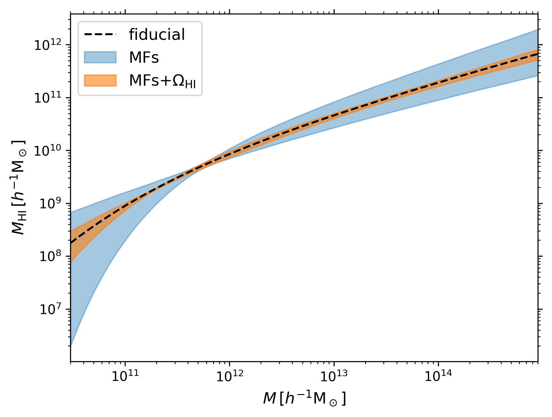
In figure 7, we show that the MFs and $\Omega_{\mathrm{HI}}$ are very informative regarding the halo occupation properties of HI. The posterior distribution of the mean HIHMR shows little scatter around the fiducial model. Uncertainties on $M_{\mathrm{HI}}$ are particularly small for halo masses $M\simeq 10^{12}\,h^{-1}$ M_⊙ (which corresponds to a few $M_{\mathrm{min}}$ and identifies the haloes containing most HI) and increase as one moves away in both directions.

Figure 5: The relative marginalised uncertainty (68.3 per cent credibility interval) for each model parameter as a function of $t_{\mathrm{pix}}$. The orange lines and shaded regions show the mean and rms scatter of the results over the 30 noise realisations. They refer to the combination of the MFs with the $\Omega_{\mathrm{HI}}$ data. The blue lines show the mean uncertainty when only the MFs are considered (in order to improve readability, we do not show the scatter which is similar to the previous case). Finally, the dotted and dashed lines indicate the results obtained in the absence of thermal noise, i.e. in the limit $t_{\mathrm{pix}}\to\infty$.

Figure 6: Joint marginalised $68.3$ per cent and $95.4$ per cent credible regions for all pairs of model parameters that determine the HIHMR. The figure refers to a particular realisation of thermal noise obtained assuming $t_{\mathrm{pix}}=3.9\times 10^{4}$ s. Dashed ellipses show the results obtained from the Fisher information matrix for the MFs while shaded ellipses refer to the combination with measurements of $\Omega_{\mathrm{HI}}$.

Figure 7: Central 68.3 per cent credibility interval of the mean HIHMR at $z=1$ obtained by fitting the MFs (light blue) and their combination with estimates of $\Omega_{\mathrm{HI}}$ (orange) in a single frequency channel at $z=1$. This result is obtained by marginalising equation (1) over the posterior distribution of the model parameters shown in figure 6, and thus assumes $t_{\mathrm{pix}}=3.9\times 10^{4}$ s. The dashed curve indicates the fiducial relation.

Table 1: Fiducial values and forecast uncertainties for the model parameters that regulate the HIHMR. The top section gives the results from the Fisher-information analysis for one channel at $z=1$. The bottom sections refer to fits of either second-order polynomials, $\theta(z)=\theta_{0}+\theta_{1}\,(z-1)+\theta_{2}\,(z-1)^{2}$ or constants, $\theta(z)=\theta_{0}$, to the measurements in the data cubes for $0.5<z<1.5$. The optimistic case (opt) treats all channels as independent data points while the pessimistic one (pes) considers only one channel every five.

	$\alpha$				$M_{0}$				$M_{\rm min}$				$\gamma$
					$[10^{10}h^{-1}\,\mathrm{M}_{\odot}]$				$[10^{11}h^{-1}\,\mathrm{M}_{\odot}]$
Fiducial value $\theta$	0.53				1.50				6.00				0.35
$\Delta\theta$ single channel	0.05				0.15				0.23				0.11
	$\theta_{0}$	$\theta_{1}$	$\theta_{2}$		$\theta_{0}$	$\theta_{1}$	$\theta_{2}$		$\theta_{0}$	$\theta_{1}$	$\theta_{2}$		$\theta_{0}$
Fiducial value $\theta_{i}$	0.53	0.20	-0.06		1.50	-1.49	1.38		6.00	-8.21	6.02		0.35
$\Delta\theta_{i}$ data cube (opt)	0.01	0.01	0.06		0.02	0.05	0.16		0.02	0.07	0.23		0.01
$\Delta\theta_{i}$ data cube (pes)	0.01	0.03	0.11		0.03	0.09	0.33		0.05	0.15	0.49		0.02

5.3 Constraints from the full data cube

So far, we have focused on a single frequency channel corresponding to a narrow redshift bin centered around $z=1$ and constrained the HIHMR using the MFs of the two-dimensional HI intensity map. We want now to make use of the full data cube that the radio observations will provide. With this aim in mind, we imagine to repeat the measurement of the MFs in each frequency channel and then fit the redshift evolution of the model parameters. In fact, it is reasonable to expect that the parameters of the HIHMR should vary smoothly with redshift. In order to exemplify the power of this technique, we synthesize the data at $z\simeq 1$ in table 1 of Villaescusa-Navarro et al. (2018) in terms of the second-order Taylor expansions

$$\alpha =0.53+0.18\,(z-1)-0.11\,(z-1)^{2}\;,$$ (26)

$$M_{0} =[1.5-1.5\,(z-1)+1.3\,(z-1)^{2}]\times 10^{10}\,h^{-1}\,\mathrm{M}_{\odot}\;,$$ (27)

$$M_{\mathrm{min}} =[6.0-8.2\,(z-1)+5.8\,(z-1)^{2}]\times 10^{11}\,h^{-1}\,\mathrm{M}_{\odot}\;,$$ (28)

$$\gamma =0.35\;,$$ (29)

and use them as the fiducial model for the evolution of the HIHMR in the redshift range $0.5<z<1.5$. This interval contains 189 channels with $\Delta\nu=2$ MHz. We can measure the MFs in each of them and then fit the marginalised constraints on the individual model parameters with second-order polynomials of $z-1$. Results obtained by assuming independent data points are reported in table 1. Since the thickness of each channel along the line of sight is only a few times larger than the correlation length of the density field and redshift-space distortions can also shift HI by comparable distances, it might be inappropriate to consider the results obtained from consecutive channels as independent. We thus repeat the analysis by considering only one channel every five. Of course, the uncertainty on the model parameters slightly increases in this case (see table 1). Note that, if we compare the results obtained for $z=1$ from the multi-channel fits to those presented in section 5.2, we note an improvement of the error bars up to a factor of ten.

6 Discussion

It has been shown that the MFs are powerful data-analysis tools to characterise –and extract information from– various cosmological datasets. However, they are sub-optimal in the case of Gaussian random fields for which the whole statistical information is contained in the power spectrum. In fact, many of the practical issues associated with the MFs (dealing with a masked sky, modelling the impact of noise) are solved problems for inferences based on power spectra. A question then naturally arises: are the fluctuations in the 21-cm-brightness-temperature distribution departing from a Gaussian random field so that to justify the use of the MFs in our study? This question is particularly relevant given the large beam of the SKA-1 MID telescopes which corresponds to a transverse size of approximately 50 comoving Mpc at $z=1$ (that we use in combination with frequency channels that extend for nearly 13 comoving Mpc along the line of sight).

In figure 8, we show the probability density function (PDF) of the brightness temperature extracted from our simulation box in the absence of thermal noise (i.e. assuming $t_{\mathrm{pix}}\rightarrow\infty$). In order to facilitate visual comparison with the Gaussian case, we also plot a normal distribution with the same mean and standard deviation as the simulated data (solid line). The PDF of the brightness temperature is clearly asymmetric (with a skewness of $1.04\pm 0.01$) and has heavier tails than a Gaussian distribution (with a kurtosis of $0.708\pm 0.006$)

It is also interesting to check how much the MFs in the mock maps depart from the expected values for a Gaussian random field. Analytical formulae have been derived for the MFs of a Gaussian random field on the Euclidean plane or on the two sphere (see section 4.1). However, important corrections need to be applied when the domain of the random field is a small subset of the above mentioned spaces. Moreover, the overall normalisation of the curves $V_{i}(\tau)$ depends on the power spectrum of the random field. For these two reasons, we compute the Gaussian MFs by averaging over many realisations obtained by shuffling the phases between the Fourier modes of the simulated data (in the absence of thermal noise, as in figure 3). Our results are shown in figure 9. While the surface area $V_{0}(\tau)$ covered by the excursion set is hardly distinguishable from the Gaussian case, larger differences are noticeable for the perimeter of the boundary $V_{1}(\tau)$ and for the Euler characteristic, in particular, for extreme values of the threshold parameter $\tau$ both on the low and high sides.

A related issue is whether the information encoded in the MFs on the large scales probed by the SKA-1 MID is enough to constrain all the parameters that influence the mean HIHMR. In fact, by reasoning in terms of the halo model (see Cooray & Sheth, 2002, for a review), one expects the data to be fully in the so-called ‘two-halo’ regime where all the information about the HIHMR is collapsed into the linear bias parameter of the HI with respect to the mass. Effectively, this would mean that the exercise we are proposing tries to constrain several parameters from the measurement of a single quantity. This line of reasoning assumes that the bias relation between HI and matter fluctuations is linear on scales of 10-50 Mpc. It is well known, however, that this is only true to first approximation. Several non-linear corrections are needed to accurately model the spatial distribution of dark-matter haloes, especially when one considers statistics that are more sensitive to non-Gaussian features than the power spectrum. State-of-the-art models include, at least, extra terms that scale quadratically with the matter density or linearly with the tidal field (see e.g. Desjacques et al., 2018, for a review). Our results can thus be interpreted as providing evidence that the same corrections are needed to describe the non-Gaussian features of the HI distribution. Further evidence has been recently provided by Cunnington et al. (2021) in a study of the bispectrum of 21-cm intensity maps. Nevertheless, some level of degeneracy between the model parameters is indeed present in our results, as shown in figure 6. This is mostly broken when independent measurements of the HI abundance are considered in combination with the MFs.

Figure 8: The PDF of the brightness-temperature fluctuations in our mock maps (shaded histogram) is contrasted with a Gaussian distribution with the same mean and variance.

Figure 9: The mean MFs (solid) and their rms scatter (shaded region) extracted from our simulations in the absence of thermal noise are compared with the mean signal for a Gaussian random field with the same power spectrum and domain (dotted lines).

7 summary

Determining the overall content and the spatial distribution of HI in the post-reionization Universe is pivotal to understand galaxy formation and evolution. An important step in this direction is the determination of the HIHMR which gives the mean and scatter of the total HI mass contained within a dark-matter halo of mass $M$. In this paper, we have investigated the possibility of constraining parametric models of the HIHMR from 21 cm intensity maps at redshift $z\simeq 1$. In particular, we have used the geometry and topology of the maps as quantified by the MFs of the brightness-temperature isocontours.

For practical reasons, we have considered a specific parameterization for the HIHMR in which the mean HI mass at fixed halo mass is given by equation (1) and a lognormal scatter of size $\sigma$ is assumed (see section 2.2). By assuming a set of fiducial values based on previous numerical studies, we have generated mock data from a large N-body simulation and used the Fisher information matrix to derive the forecast constraints on the model parameters. As a reference case, we have considered the SKA-1 MID dark-energy survey at $z=1$ (conducted in single-dish mode) and assumed frequency channels of width $\Delta\nu=2$ MHz.

Our main results can be summarised as follows.

1. After subtracting the foregrounds, the 21 cm signal is of the order of a few mK, nearly 1000 times lower than the system temperature of the telescopes. In order to beat thermal noise and reach the sensitivity necessary for imaging the HI distribution, long integration times per pixel, $t_{\mathrm{pix}}$, are thus required. By using the MFs of the 21 cm intensity map in a single frequency channel, we find that the parameters of the HIHMR can be measured with a signal-to-noise ratio of one if $t_{\mathrm{pix}}\simeq 9.8\times 10^{3}$ s. Nearly optimal error bars are obtained using $t_{\mathrm{pix}}\simeq$ a few $\times 10^{4}$ s. This corresponds to a total observing time of 4 - 5 days.

2. Information on the mean HI density, $\Omega_{\mathrm{HI}}$, is lost during the foreground removal from the intensity maps. This loss can be restored by combining the MFs with independent measures of $\Omega_{\mathrm{HI}}$. This addition slightly improves the constraints on some of the parameters that regulate the HIHMR, in particular on the slope $\alpha$ defined in equation (1).

3. The mean HIHMR is very tightly constrained for haloes with $M\simeq 10^{12}h^{-1}$ M_⊙ which contain most of the HI at $z=1$. Uncertainties grow larger as both larger and smaller halo masses are considered.

4. Combining measurements of the MFs in different frequency channels provides exquisite constraints on the redshift evolution of the HIHMR (both for the mean and the scatter), especially for redshifts that lie around the center of the data cube along the frequency axis. In this case, we forecast uncertainties on the model parameters that are an order of magnitude smaller with respect to those extracted from a single channel.

In this paper, we have used the SKA-1 MID dark-energy survey as an example of what can be achieved with forthcoming facilities. Observations at higher angular resolution with SKA precursors like the Hydrogen Intensity and Real-time Analysis eXperiment (HIRAX, Newburgh et al., 2016) in the southern hemisphere and the Canadian Hydrogen Intensity Mapping Experiment (CHIME, Bandura et al., 2014) in the northern hemisphere will probe length scales at which the HI-to-mass bias relation is more non-linear. Given long enough integration times, these experiments might be able to partially remove the degeneracy among the model parameters of the HIHMR and even constrain them more tightly. We will investigate this possibility in our future work.

Data availability statement

The data underlying this article will be shared on reasonable request to the corresponding author.

References

- Adler (1981) Adler R. J., 1981, The Geometry of Random Fields. John Wiley & Sons, Chichester
- Ai & Zhu (2018) Ai M., Zhu M., 2018, ApJ, 862, 48
- Alonso et al. (2017) Alonso D., Ferreira P. G., Jarvis M. J., Moodley K., 2017, Phys. Rev. D, 96, 043515
- Ando et al. (2019) Ando R., Nishizawa A. J., Hasegawa K., Shimizu I., Nagamine K., 2019, MNRAS, 484, 5389
- Bagla et al. (2010) Bagla J. S., Khandai N., Datta K. K., 2010, MNRAS, 407, 567
- Bandura et al. (2014) Bandura K., et al., 2014, Ground-based and Airborne Telescopes V
- Barkana & Loeb (2005) Barkana R., Loeb A., 2005, ApJ, 626, 1
- Barnes & Haehnelt (2014) Barnes L. A., Haehnelt M. G., 2014, MNRAS, 440, 2313
- Baugh et al. (2019) Baugh C. M., et al., 2019, MNRAS, 483, 4922
- Bull et al. (2015) Bull P., Ferreira P. G., Patel P., Santos M. G., 2015, Astrophysics Journal, 803
- Chen et al. (2019) Chen Z., Xu Y., Wang Y., Chen X., 2019, ApJ, 885, 23
- Chen et al. (2020) Chen T., Battye R. A., Costa A. A., Dickinson C., Harper S. E., 2020, MNRAS, 491, 4254
- Cooray & Sheth (2002) Cooray A., Sheth R., 2002, Phys. Rep., 372, 1
- Crain et al. (2017) Crain R. A., et al., 2017, MNRAS, 464, 4204
- Crighton et al. (2015) Crighton N. H. M., et al., 2015, MNRAS, 452, 217
- Cunnington et al. (2019) Cunnington S., Harrison I., Pourtsidou A., Bacon D., 2019, MNRAS, 482, 3341
- Cunnington et al. (2021) Cunnington S., Watkinson C., Pourtsidou A., 2021, arXiv e-prints, p. arXiv:2102.11153
- Davé et al. (2013) Davé R., Katz N., Oppenheimer B. D., Kollmeier J. A., Weinberg D. H., 2013, MNRAS, 434, 2645
- Desjacques et al. (2018) Desjacques V., Jeong D., Schmidt F., 2018, Phys. Rep., 733, 1
- Di Matteo et al. (2002) Di Matteo T., Perna R., Abel T., Rees M. J., 2002, ApJ, 564, 576
- Efstathiou (1992) Efstathiou G., 1992, MNRAS, 256, 43P
- Giovanelli et al. (2005) Giovanelli R., et al., 2005, AJ, 130, 2598
- Gleser et al. (2006) Gleser L., Nusser A., Ciardi B., Desjacques V., 2006, MNRAS, 370, 1329
- Gott et al. (1990) Gott J. Richard I., Park C., Juszkiewicz R., Bies W. E., Bennett D. P., Bouchet F. R., Stebbins A., 1990, ApJ, 352, 1
- Guo et al. (2020) Guo H., Jones M. G., Haynes M. P., Fu J., 2020, ApJ, 894, 92
- Hadwiger (1957) Hadwiger H., 1957, Vorlesungen ueber Inhalt, Oberflache und Isoperimetrie. Springer
- Hall (2005) Hall P. J., 2005, The Square Kilometre Array: An Engineering Perspective
- Hallinan et al. (2019) Hallinan G., et al., 2019, in Bulletin of the American Astronomical Society. p. 255 (arXiv:1907.07648)
- Hartlap et al. (2007) Hartlap J., Simon P., Schneider P., 2007, A&A, 464, 399
- Hong et al. (2010) Hong S. E., Ahn K., Park C., Kim J., Iliev I. T., Mellema G., 2010, 2D Genus Topology of 21-cm Differential Brightness Temperature During Cosmic Reionization (arXiv:1008.3914)
- Hu et al. (2019) Hu W., et al., 2019, MNRAS, 489, 1619
- Kanekar et al. (2016) Kanekar N., Sethi S., Dwarakanath K. S., 2016, ApJ, 818, L28
- Kapahtia et al. (2018) Kapahtia A., Chingangbam P., Appleby S., Park C., 2018, J. Cosmology Astropart. Phys., 2018, 011
- Kaufman (1967) Kaufman G., 1967, Center for Operations Research and Econometrics Discussion Paper
- Kim et al. (2017) Kim H.-S., Wyithe J. S. B., Baugh C. M., Lagos C. d. P., Power C., Park J., 2017, MNRAS, 465, 111
- Klypin et al. (2016) Klypin A., Yepes G., Gottlöber S., Prada F., Heß S., 2016, MNRAS, 457, 4340
- Loeb & Wyithe (2008) Loeb A., Wyithe J. S. B., 2008, Phys. Rev. Lett., 100, 161301
- Mantz et al. (2008) Mantz H., Jacobs K., Mecke K., 2008, Journal of Statistical Mechanics: Theory and Experiment, 2008, 12015
- Marr et al. (2015) Marr J., Snell R., Kurtz S., 2015, Fundamentals of Radio Astronomy: Observational Methods. Series in Astronomy and Astrophysics, CRC Press, https://books.google.de/books?id=T54oCwAAQBAJ
- Matsubara (2003) Matsubara T., 2003, Astrophysics Journal, 584, 1
- Mecke et al. (1994) Mecke K. R., Buchert T., Wagner H., 1994, A&A, 288, 697
- Minkowski (1903) Minkowski H., 1903, Mathematische Annalen, 57, 447
- Monsalve et al. (2019) Monsalve R. A., Fialkov A., Bowman J. D., Rogers A. E. E., Mozdzen T. J., Cohen A., Barkana R., Mahesh N., 2019, ApJ, 875, 67
- Neeleman et al. (2016) Neeleman M., Prochaska J. X., Ribaudo J., Lehner N., Howk J. C., Rafelski M., Kanekar N., 2016, ApJ, 818, 113
- Newburgh et al. (2016) Newburgh L. B., et al., 2016, in Hall H. J., Gilmozzi R., Marshall H. K., eds, Society of Photo-Optical Instrumentation Engineers (SPIE) Conference Series Vol. 9906, Ground-based and Airborne Telescopes VI. p. 99065X (arXiv:1607.02059), doi:10.1117/12.2234286
- Novikov et al. (1999) Novikov D., Feldman H. A., Shandarin S. F., 1999, International Journal of Modern Physics D, 8, 291
- Novikov et al. (2000) Novikov D., Schmalzing J., Mukhanov V. F., 2000, A&A, 364, 17
- Obuljen et al. (2019) Obuljen A., Alonso D., Villaescusa-Navarro F., Yoon I., Jones M., 2019, MNRAS, 486, 5124
- Oh & Mack (2003) Oh S. P., Mack K. J., 2003, MNRAS, 346, 871
- Padmanabhan & Refregier (2017) Padmanabhan H., Refregier A., 2017, MNRAS, 464, 4008
- Padmanabhan et al. (2015) Padmanabhan H., Choudhury T. R., Refregier A., 2015, MNRAS, 447, 3745
- Padmanabhan et al. (2017) Padmanabhan H., Refregier A., Amara A., 2017, MNRAS, 469, 2323
- Papastergis et al. (2013) Papastergis E., Giovanelli R., Haynes M. P., Rodríguez-Puebla A., Jones M. G., 2013, ApJ, 776, 43
- Paul et al. (2018) Paul N., Choudhury T. R., Paranjape A., 2018, MNRAS, 479, 1627
- Péroux & Howk (2020) Péroux C., Howk J. C., 2020, ARA&A, 58, 363
- Planck Collaboration et al. (2014) Planck Collaboration et al., 2014, A&A, 571, A16
- Pontzen et al. (2008) Pontzen A., et al., 2008, MNRAS, 390, 1349
- Pranav et al. (2019) Pranav P., et al., 2019, Monthly Notices of the Royal Astronomical Society, 485, 4167–4208
- Rao et al. (2006) Rao S. M., Turnshek D. A., Nestor D. B., 2006, ApJ, 636, 610
- Rao et al. (2017) Rao S. M., Turnshek D. A., Sardane G. M., Monier E. M., 2017, MNRAS, 471, 3428
- Rees (1986) Rees M. J., 1986, MNRAS, 218, 25P
- Schmalzing & Buchert (1997) Schmalzing J., Buchert T., 1997, ApJ, 482, L1
- Schmalzing & Gorski (1998) Schmalzing J., Gorski K. M., 1998, MNRAS, 297, 355
- Scoccimarro et al. (2001) Scoccimarro R., Sheth R. K., Hui L., Jain B., 2001, ApJ, 546, 20
- Seehars et al. (2016) Seehars S., Paranjape A., Witzemann A., Refregier A., Amara A., Akeret J., 2016, J. Cosmology Astropart. Phys., 2016, 001
- Shaver et al. (1999) Shaver P. A., Windhorst R. A., Madau P., de Bruyn A. G., 1999, A&A, 345, 380
- Slosar et al. (2019) Slosar A., et al., 2019, in Bulletin of the American Astronomical Society. p. 53 (arXiv:1907.12559)
- Spinelli et al. (2020) Spinelli M., Zoldan A., De Lucia G., Xie L., Viel M., 2020, MNRAS, 493, 5434
- Square Kilometre Array Cosmology Science Working Group et al. (2018) Square Kilometre Array Cosmology Science Working Group et al., 2018, arXiv e-prints, p. arXiv:1811.02743
- Switzer et al. (2013) Switzer E. R., et al., 2013, MNRAS, 434, L46
- Tomita (1990) Tomita H., 1990, Kawasaki K., Suzuki M., and Onuki A. (eds.), Formation, dynamics and statistics of patterns, Vol. 1, pp 113–157. World Scientific
- Vanderlinde et al. (2019) Vanderlinde K., et al., 2019, in Canadian Long Range Plan for Astronomy and Astrophysics White Papers. p. 28 (arXiv:1911.01777), doi:10.5281/zenodo.3765414
- Villaescusa-Navarro et al. (2014) Villaescusa-Navarro F., Viel M., Datta K. K., Choudhury T. R., 2014, J. Cosmology Astropart. Phys., 2014, 050
- Villaescusa-Navarro et al. (2018) Villaescusa-Navarro F., et al., 2018, The Astrophysical Journal, 866, 135
- Wolz et al. (2015) Wolz L., et al., 2015, in Advancing Astrophysics with the Square Kilometre Array (AASKA14). p. 35 (arXiv:1501.03823)
- Yue & Ferrara (2019) Yue B., Ferrara A., 2019, MNRAS, 490, 1928
- Zaldarriaga et al. (2004) Zaldarriaga M., Furlanetto S. R., Hernquist L., 2004, ApJ, 608, 622
- Zoldan et al. (2017) Zoldan A., De Lucia G., Xie L., Fontanot F., Hirschmann M., 2017, MNRAS, 465, 2236