Synthetic Multidimensional Plasma Electron Hole Equilibria

Abstract

Methods for constructing synthetic multidimensional electron hole equilibria without using particle simulation are investigated. Previous approaches have various limitations and approximations that make them unsuitable within the context of expected velocity diffusion near the trapped-passing boundary. An adjustable model of the distribution function is introduced that avoids unphysical singularities there, and yet is sufficiently tractable analytically to enable prescription of the potential spatial profiles. It is shown why simple models of the charge density as being a function only of potential cannot give solitary multidimensional electron holes, in contradiction of prior suppositions. Fully self-consistent axisymmetric electron holes in the drift-kinetic limit of electron motion (negligible gyro-radius) are constructed and their properties relevant to observational interpretation and finite-gyro-radius theory are discussed.

I Introduction

Active space plasma regions are observed to contain long-lived solitary positive potential peaks whose spatial extent is a few Debye lengths; they are mostly identified as electron holes, having an electron charge deficit on trapped orbitsMatsumoto et al. (1994); Ergun et al. (1998); Bale et al. (1998); Mangeney et al. (1999); Pickett et al. (2008); Andersson et al. (2009); Wilson et al. (2010); Malaspina et al. (2013, 2014); Vasko et al. (2015); Mozer et al. (2016); Hutchinson and Malaspina (2018); Mozer et al. (2018). It has been known for a long time that non-zero magnetic field is necessary for the sustainment of electron holes; if it is strong enough, the electron motion and trapping becomes one-dimensional. One-dimensional dynamic treatments have predominated past hole theory, where the gyro-radius $r_{L}$ is neglected relative to the transverse scale length $L_{\perp}$. Although the present theory continues to calculate using only parallel particle dynamics, it takes account qualitatively of one recently discovered important effect of the transverse electric field in a multidimensional electron hole, namely the resonant interaction of the trapped particle bounce motion with the gyro-motion. This interaction essentially always induces a region of stochastic orbits near zero parallel energy: the trapped-passing boundary of phase space. And the energy-depth of this stochastic layer increases with $r_{L}/L_{\perp}$Hutchinson (2020). The anticipated result in the stochastic layer is a large effective phase-space diffusion rate which forces the distribution function (phase-space density) to be approximately independent of energy in that region. It has also been shown recentlyHutchinson (2021), in contradiction of a longstanding suggestion, that regardless of the relative strength of the magnetic field, the screening of the trapped electron deficit charge is isotropic: having approximately Boltzmann dependence. This discredits one speculation concerning how the transverse scale of electron holes relates to magnetic field strength, and reemphasizes the need to understand better multidimensional electron holes, especially since recent multi-satellite measurements are giving unprecedented information about multidimensional holes in space plasmas.

The purpose of the present work is to develop a versatile model of self-consistent multidimensional electron hole equilibria that conform to the physical constraint of having zero distribution slope at and for a controllable depth inside the trapped-passing boundary. Because of the difficulties of taking fully into account finite gyro-radius dynamic effects, the model simply prescribes the parallel velocity distribution as a function of transverse position $r$, and potential $\phi$. This exactly represents the electron dynamics only for the limit of high magnetic field (one-dimensional motion) where the gyro-radius is small. However, even this first step has not previously been achieved taking properly into account the full Poisson equation and resulting non-separable form of its solution for the potential. The present results provide physically self-consistent potential profiles in which the consequences of transverse dynamics, and especially gyro-averaging, will be explored in a separate publication. An illustrative equilibrium found by the present approach (explained fully later) is shown in Fig. 1.

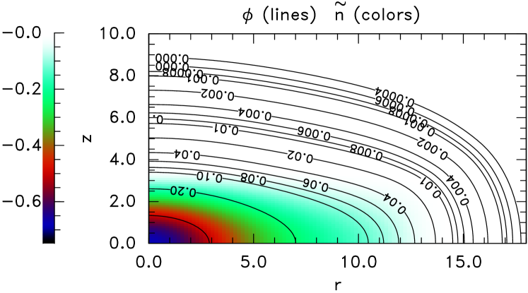
Figure 1: An oblate electron hole equilibrium, axisymmetric about the magnetic field direction $z$, showing color contours of the trapped electron density deficit $\tilde{n}$, and line contours of the self-consistent potential $\phi$.

After a review of prior analysis of multidimensional electron hole equilibria (section 2), a model distribution function with shape controlled by adjustable parameters is introduced in section 3. It avoids the unphysical properties of most previous choices, and from it explicit analytic expressions for the charge deficit and (for some parameters) the one-dimensional potential profile can be derived. It is generalized to separable multidimensional potential forms. In section 4 is explained the subtlety of how to relax the potential iteratively to the non-separable form it always must take. It becomes clear that no solitary multidimensional equilibrium can in fact exist when the charge density is a function only of potential. It must be also an explicit function of transverse position. Iterative relaxation with effectively constant trapped charge deficit embodies sufficient of the physical stabilizing dynamics to produce a convergent scheme. And examples of hole shapes are examined with particular emphasis on the consequences for satellite observations.

For convenience throughout this paper normalized units are used: Debye-length $\lambda_{D}$ for length, inverse plasma frequency $1/\omega_{pe}$ for time, and background temperature $T_{e\infty}$ for energy; with the result that velocity units are $\sqrt{T_{e\infty}/m_{e}}$. Densities are normalized to the distant background electron density $n_{e\infty}$. In steady state, the total energy $W=v^{2}/2-\phi$ (normalized units) of an electron is conserved, and neglecting collisions, the total derivative of the distribution function $df(v)/dt$ along particle orbits is zero. Ions are taken to be a uniform immobile neutralizing background.

II Two dimensional hole equilibria

Electron holes are a type of BGK equilibriumBernstein, Greene, and Kruskal (1957) in which a deficit of the electron velocity distribution on trapped orbits sustains the positive potential that traps them. For decades electron hole analysis was almost all one-dimensional, along the magnetic field and ignored or highly simplified any transverse spatial dependence. This one-dimensional prior theory has been reviewed extensively elsewhereTurikov (1984); Schamel (1986); Eliasson and Shukla (2006); Hutchinson (2017) and will not be discussed in detail here, but a brief review of the relatively few multidimensional electron hole analytic equilibrium studies is appropriate.

Multidimensional electrostatic hole model studies were published for several years following 2000, motivated by new observational data documenting finite transverse hole extent in space plasmas. The model equilibria based their particle dynamics on the one-dimensional Vlasov equation plus drift in a uniform magnetic field, but began to account for transverse potential variation, generally simplifying the problem to axisymmetric cases (independent of $\theta$ in cylindrical coordinates, which is our focus here too).

Chen and Parks (2002) specified the potential to have a separable axisymmetric form and a constant value of $\nabla_{\perp}^{2}\phi/\phi$ , giving $\phi=\phi_{\parallel}(z)J_{0}(l_{0}r/r_{s})$ ( the Bessel function $J_{0}$ has its first zero at argument $l_{0}$). The potential is thus zero, but has finite $\nabla_{\perp}$, at $r=r_{s}$. This represents a “waveguide” configuration, effectively equivalent to the (1979) analysis of SchamelSchamel (1979), rather than an isolated hole far from boundaries. The convenience of the ansatz is that the Laplacian in Poisson’s equation simply acquires from transverse divergence an extra term $k_{\perp}^{2}\phi$ where $k_{\perp}^{2}=(l_{0}/r_{s})^{2}$ is independent of $r$. This term is readily included into an expression for charge density in Poisson’s equation. With potential specified in this way, and an assumed Maxwellian untrapped distribution, the authors solve the integral equation for the trapped parallel distribution function $f_{\parallel}(W_{\parallel})$ (for parallel energy including potential $W_{\parallel}<0$). One commonly discussed criterion is that $f_{\parallel}$ must be non-negative, which constrains the hole parallel length in a way that depends on the perpendicular scale $r_{s}$.

Later, Chen, Thouless, and Tang (2004) analyzed instead Gaussian potential shapes $\phi\propto\exp(-z^{2}/\delta_{z}^{2}-r^{2}/\delta_{\perp}^{2})$ (still separable but far from boundaries), showing that the required trapped density as a function of potential, and trapped distribution as a function of energy, can be derived in closed form for Maxwellian background distribution. They also included the static response of a repelled (ion) Maxwellian species of different temperature.

Muschietti et al. (2002) prescribed a separable potential $\phi\propto[1+\eta\cosh(\beta z)]^{-1}\exp[-(r/\delta_{\perp})^{2}]$, which allows parallel elongation of the hole by flattening its top via the parameter $\eta$, and prescribing its asymptotic scale-length $1/\beta$ at large $z$. Its perpendicular variation is Gaussian, which means that writing $\nabla_{\perp}^{2}\phi(z)=k_{\perp}^{2}\phi$, implies $k_{\perp}^{2}$ varies with $r$. By making a mathematically convenient (non-Maxwellian) choice of the external parallel distribution, they found a closed analytic form for the trapped distribution, satisfying the parallel integral equation self-consistently as a function of energy and radius $r$. This calculation (like those of Chen et al) is carried out in the drift kinetic approximation, assuming the ordering $\omega_{\theta}\ll\omega_{b}\ll\Omega_{e}$ where $\omega_{\theta}$ is the azimuthal drift frequency of the gyrocenter about the axis, $\omega_{b}$ is the parallel bounce frequency, and $\Omega_{e}$ the cyclotron frequency. It also ignores the distinction between guiding-center density and particle density, effectively neglecting the gyro radius relative to the perpendicular scale length. The work explores only limited transverse extent $r/\delta_{\perp}\leq 1.3$.

These three early papers using the “integral equation” solution approach (prescribing the parallel potential shape) all have a slope singularity in the parallel distribution function at the separatrix where the parallel energy $W_{\parallel}$ is zero, $f_{\parallel}(W_{\parallel})-f_{\parallel}(0)\propto(-W_{\parallel}/\psi)^{1/2}$, which Muschietti et al illustrate. And they all use separable potential form.

Jovanović et al. (2002) approached the problem instead by the “differential equation” route, specifying the trapped parallel distribution function to be of the Schamel form ($\propto\exp(\beta W_{\parallel}/T)$), which for small potential gives a density difference from pure Debye shielding (i.e. $n_{e}/n_{0}=1+\phi$) proportional to $-\phi^{3/2}$, and no $f_{\parallel}$-slope singularity. They supposed that the Poisson equation was modified by anisotropic dielectric shielding, becoming effectively $\{\nabla_{\parallel}^{2}+[1+(\omega_{p}/\Omega_{e})^{2}\nabla_{\perp}^{2}]\}\phi=a\phi-(4b/3)\phi^{3/2}$. This supposed modification of Poisson’s equation is erroneous when applied to electron holes, as has been shown elsewhereHutchinson (2021).

Krasovsky, Matsumoto, and Omura (2004a) show that in a plasma with (Debye) shielding length $\lambda_{D}$, a spherically symmetric hole of Gaussian form $\phi=\psi\exp(-R^{2}/\lambda^{2})$ is self-consistent with a trapped parallel distribution function deficit $\tilde{f}_{\parallel}=f_{\parallel trapped}(W_{\parallel})-f_{\parallel}(0)=-(2|W_{\parallel}|/\pi^{2})^{1/2}[1/\lambda_{D}^{2}+(2/\lambda^{2})(1+2\ln(4|W_{\parallel}|/\psi)]$, governed by the Vlasov equation. For mathematical convenience, they invoke instead the presumption that the trapped particle density (deficit), like the shielding density, depends linearly on the potential, which is satisfied by having $\tilde{f}_{\parallel}\propto\sqrt{W_{j}-W_{\parallel}}$ for $W_{\parallel}/W_{j}>1$ and zero for $W_{\parallel}/W_{j}<1$, where $W_{j}=-\phi_{j}$ is some maximum trapped energy ($W_{j}<0$). The advantage is that the linear dependence of density gives rise to Helmholtz’s equation $(\nabla^{2}+k^{2})(\phi-const.)=0$ except with the constant $k^{2}=-dn/d\phi$ different (in magnitude and sign) in the two regions $W_{\parallel}/W_{j}\lessgtr 1$. The potential in the inner region can be expressed in terms of a sum of known harmonic solutions, by specifying the position in $r$ and $z$ of the potential contour at the join $\phi=\phi_{j}$.

In Krasovsky, Matsumoto, and Omura (2004b) these authors venture beyond the pure drift approximation, noting that a potential of the additive form $\phi=\psi\times[1-(z/L)^{2}-(r/R)^{2}]$ gives rise to integrable equations of motion. Although they do not find an equilibrium, they note that the resulting (2-D) Vlasov equation is satisfied by $f(v)$ being an arbitrary function of the energy-like constants of the motion, $w_{\parallel}=v_{z}^{2}/2+(z/L)^{2}\psi$, and $w_{\perp}=v_{r}^{2}/2+(r/R)^{2}\psi+(p_{\theta}/r+Br/2)^{2}/2$, where $p_{\theta}$ is the conserved canonical angular momentum about the axis of symmetry in the magnetic field $B$, and the total energy is actually $W=w_{\perp}+w_{\parallel}-\psi$. They concentrate on the density at $r=0$, $z=0$, noting that orbits that pass through the origin have $p_{\theta}=0$, and are trapped only if they never reach $\phi=0$, which is true if $W_{\parallel}+1/[1+(BR)^{2}/8\psi]W_{\perp}<\psi$. This inequality defines the interior of a trapped ellipse in velocity space at the origin, and thereby limits the maximum possible charge deficit contributable by trapped particles. To make that exceed the passing particle density perturbation (which at a minimum it must), when the field is weak $B\lesssim 1$ and $\psi\ll B$, they show requires $(r_{L}/R)^{2}\sqrt{\psi}\lesssim 1$. Thus, a maximum thermal gyro radius $r_{Le}$ of order the hole’s radial scale length ($R$) times $\psi^{-1/4}$ is permitted. A similar criterion is derived by Krasovsky et al (2006).

After 2006 I am aware of no published analytic assaults on the multi-dimensional hole equilibrium problem until Hutchinson (2020) showed that when transverse potential gradients exist there is always a region of stochastic orbits caused by bounce-cyclotron resonance near $W_{\parallel}=0$. The energy depth of the stochastic region is found as a function of the peak potential $\psi$, $E_{\perp}$, and the magnetic field strength $B$. It deepens rapidly when $B/\sqrt{\psi}\lesssim 2$ and $E_{\perp}$ is significant, eventually extending to the full hole depth. The presence of this stochastic region will prevent the formation of any strong energy gradients of $f_{\parallel}$ near $W_{\parallel}=0$, ruling out any distributions that do not have an approxmately flat region of $f_{\parallel}$ there. As has been noted beforeHutchinson (2017), this forces a requirement that the hole potential fall $\propto\exp(-z/\lambda_{D})$ at large z, but it also constrains $\phi\propto\exp(-r/\lambda_{D})$ at large $r$. Thus, exact Gaussian potential forms, parallel or perpendicular, cannot be physical in the hole wings.

These summaries motivate the key emphases of the present work: insisting upon physically plausible distribution dependence on energy, and abandoning the convenient but unphysical assumption that the potential form is separable. Observing these principles we construct truly physical multidimensional electron hole equilibria, based for the first time on synthetic analysis rather than particle-in-cell simulation.

III Power trapped distribution deficit model

Consider a solitary potential peak which in its own frame of reference is time-independent. The distribution function satisfying the (parallel) Vlasov equation is constant on particle orbits. Since the potential is steady, energy is also constant on orbits, and in the drift approximation in a uniform magnetic field the distribution is a function of parallel ($W_{\parallel}=v_{\parallel}^{2}/2-\phi$) and total ($W$) energy, with those energies conserved.

However, for orbits that are weakly trapped, conservation of magnetic moment (and hence of $W_{\parallel}$ separately from $W=W_{\parallel}+W_{\perp}$) begins to break down because of bounce-gyro resonanceHutchinson (2020), and resulting velocity space diffusion suppresses the difference $\tilde{f}=f_{t}-f_{\infty}(0)$ between the trapped distribution and a flat distribution having the separatrix value $f_{\infty}(0)$. We therefore adopt initially the “differential equation” ($\tilde{f}$ specified) approach to constructing a self consistent equilibrium solution. We suppose, further, that there is a bounding trapped energy $W_{j}$, lying between $-\psi$ and $0$, such that for parallel energy $W_{\parallel}>W_{j}$, $\tilde{f}$ is zero. For the more deeply trapped region where $W_{\parallel}<W_{j}$, $\tilde{f}$ is taken proportional to the energy difference raised to a chosen power $\alpha$: $\tilde{f}\propto(W_{j}-W_{\parallel})^{\alpha}$. This form is convenient because it is continuous and analytically tractable, yet enables monotonic shapes of $\tilde{f}(W_{\parallel})$ to be represented from uniform waterbag ($\alpha=0$), through rounded $\alpha\sim 1/2$ to triangular $\alpha=1$, and beyond, peaked at the maximum trapping depth. It is here called the power deficit model. We take no account of the perpendicular velocity distribution and so $f$ means $f_{\parallel}$ and we drop the parallel suffix for brevity henceforth. Fig. 2 illustrates some of the distribution function shapes that can be prescribed by the power deficit $\tilde{f}$ model.

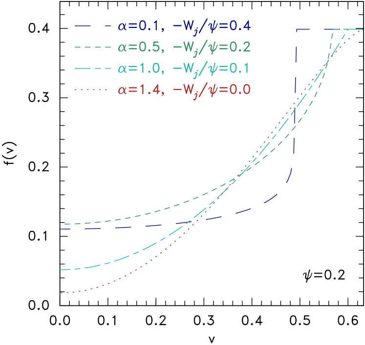
Figure 2: Illustration of shapes of the distribution function in the trapped region of velocity space at potential $\psi$, for the power deficit model.

III.1 One-dimensional

If the overall magnitude of $\tilde{f}$ is represented by its value $\tilde{f}_{\phi}$ at parallel energy $-\phi$ for some specific $\phi>-W_{j}$ (i.e. in the non-zero region), then its value at all other energies ($W_{\parallel}<W_{j}$) is

$$\tilde{f}(W_{\parallel})=\left(W_{j}-W_{\parallel}\over\phi+W_{j}\right)^{\alpha}\tilde{f}_{\phi}=C(W_{j}-W_{\parallel})^{\alpha},$$ (1)

where $C\equiv\tilde{f}_{\phi}/(\phi+W_{j})^{\alpha}$ is a constant (negative because $\tilde{f}$ is negative). We adopt for brevity hereafter the convention that energy combinations taken to some real power give zero if they are negative. The density perturbation produced by $\tilde{f}$ at potential $\phi$ is given by the integral

$$\begin{split}\tilde{n}(\phi)&=\int_{0}^{\sqrt{\phi}}\tilde{f}\,2dv=\int_{-\phi}^{W_{j}}\tilde{f}_{\phi}\left(W_{j}-W_{\parallel}\over\phi+W_{j}\right)^{\alpha}{\sqrt{2}\,dW_{\parallel}\over\sqrt{\phi+W_{\parallel}}}\\ &=2\tilde{f}_{\phi}(\phi+W_{j})^{1/2}\sqrt{2}\int_{0}^{1}(1-\zeta^{2})^{\alpha}d\zeta\\ &=2CG(\phi+W_{j})^{\alpha+1/2}\end{split}$$ (2)

[using the substitution $\zeta\equiv\sqrt{(\phi+W_{\parallel})/(\phi+W_{j})}$, and writing $G$ for the $\zeta$-integral (which is a known function of $\alpha$) $G\equiv\sqrt{2}\int_{0}^{1}(1-\zeta^{2})^{\alpha}d\zeta=\sqrt{\pi/2}\,\Gamma(\alpha+1)/\Gamma(\alpha+3/2)$].

Denote the densities due to trapped electrons $n_{t}$, passing electrons $n_{p}$, and passing plus a flat distribution of trapped electrons $n_{f}$. The charge-density $\rho=1-n_{p}-n_{t}=1-n_{f}-\tilde{n}$ is a function of $\phi$, so Poisson’s equation in one-dimension $d^{2}\phi/dz^{2}=-\rho$ can be integrated once to give

$${1\over 2}\left(d\phi\over dz\right)^{2}=\int(n_{f}-1)+\tilde{n}d\phi\equiv-V_{f}-\tilde{V}=-V_{total}.$$ (3)

For our power deficit model $\tilde{f}$ we have $-\tilde{V}=2CG(\phi+W_{j})^{\alpha+3/2}/(\alpha+3/2)$. The flat-$f$ density for a Maxwellian at small $\phi$ is $n_{f}=1+\phi$, giving (the “classical potential”) $-V_{f}=\phi^{2}/2$, and $\tilde{n}$ can be evaluated at larger $\phi$ or for other distributions, e.g. shifted Maxwellians, numerically. In any case, the implicit solution for the potential form is then $z(\phi)=\int d\phi/\sqrt{-2V_{total}}$. The crucial condition at the hole peak, $z=0$, where $d\phi/dz=0$, is then $V_{total}=0$. The peak potential $\psi=\phi(0)$ is thus the solution of

$$\begin{split}-\tilde{f}_{\psi}{2G(\psi+W_{j})^{3/2}\over\alpha+3/2}&=-2CG{(\psi+W_{j})^{\alpha+3/2}\over\alpha+3/2}\\ &=\tilde{V}(\psi)=-V_{f}(\psi).\end{split}$$ (4)

For the linear $n_{f}$ approximation $V_{f}=-\phi^{2}/2$, this equation gives

$$\tilde{f}_{\psi}/\psi^{1/2}=-{(\alpha+3/2)\over 4G}{1\over(1+W_{j}/\psi)^{3/2}},$$ (5)

which shows that $\tilde{f}_{\psi}\propto\sqrt{\psi}$ with a constant of proportionality that depends only on the $\tilde{f}$ shape parameters $\alpha$ and $W_{j}/\psi$. Also for the linear $n_{f}$ approximation

$$CG=-{(\alpha+3/2)\over 4}{\psi^{1/2-\alpha}\over(1+W_{j}/\psi)^{3/2+\alpha}};$$ (6)

so

$$\tilde{n}(\phi)=-{(\alpha+3/2)\over 2}{\psi^{2}(\phi+W_{j})^{1/2+\alpha}\over(\psi+W_{j})^{3/2+\alpha}}.$$ (7)

There does not appear to be a closed form solution for the $z(\phi)$ integral for general $\alpha$. However, as was by Krasovsky et alKrasovsky, Matsumoto, and Omura (2004a), there is when one adopts the linear $n_{f}$ approximation and $\alpha=1/2$, because the resulting linear dependence of the density on $\phi$ turns Poisson’s equation into the Helmholtz equation for $\phi>-W_{j}$ and the Modified Helmholtz equation for $\phi<-W_{j}$, which match at the join.

$$\begin{array}[]{lll}\displaystyle{d^{2}\phi\over dz^{2}}&=\phi+2CG(\phi+W_{j})\\ &=-k^{2}(\phi-2CGW_{j}/k^{2})&(-\phi<W_{j})\\ &=\phi&(-\phi>W_{j}).\end{array}$$ (8)

The inner region solution is an offset cosine:

$$\phi-2CGW_{j}/k^{2}=(\psi-2CGW_{j}/k^{2})\cos(kz)$$ (9)

where $k^{2}=-(1+2CG)$, and the amplitude comes from requiring $\phi(0)=\psi$. The outer region is an exponential

$$\phi=-W_{j}\exp(z_{j}-z).$$ (10)

The join position is where $\cos(kz_{j})=[k^{2}+2GC]/[k^{2}\psi/W_{j}+2CG]=W_{j}/[k^{2}\psi+2CGW_{j}]$. For $\alpha=1/2$ the value of $G$ is $\pi/(2\sqrt{2})$, and

$$C={\tilde{f}_{\psi}\over(\psi+W_{j})^{1/2}}={\sqrt{2}\over\pi}{1\over(1+W_{j}/\psi)^{2}}.$$ (11)

We note that there are certain constraints on allowable values of the parameters of the power deficit model. One is that the distribution function cannot be negative, so $|\tilde{f}|\leq f_{\infty}(0)=1/\sqrt{2\pi}=0.399$ (unshifted Maxwellian); this limits the allowable maximum $\psi$ to a value of order unity. Another less obvious is that for $\alpha<1/2$ there is a minimum allowable value of $-W_{j}/\psi$ for there to exist a solution to $V(\psi)=0$, and when $V_{f}=-\phi^{2}/2$ it is $-W_{j}/\psi>1/4-\alpha/2$. The minimum value $1/4$ for a waterbag $\tilde{f}$ (i.e. $\alpha\to 0$) was noted long ago by Dupree (1982).

Figure 3: Dependence of the key coefficient on power $\alpha$.

Fig. 3 shows how the numerical coefficient $4G/(\alpha+3/2)$ varies with $\alpha$. Taking into account the allowable minimum of $-W_{j}/\psi$ the maximum value of $(1+W_{j}/\psi)4G/(\alpha+3/2)$ does not rise as steeply for $\alpha<0.5$. This combination is what determines the maximum value of $\psi^{1/2}$ for a given $\tilde{f}_{\psi}$ through eq. 5, and hence how the non-negativity constraint varies with $\alpha$.

So far this is all one-dimensional analysis.

III.2 Multidimensional Generalization: Separable Potential-form

When there is transverse potential gradient, Poisson’s equation contains an additional transverse divergence term $\nabla_{\perp}^{2}\phi$ that couples together Vlasov solutions on adjacent field-lines. If its value at a certain transverse position $r$ is considered a known function of parallel position $z$, then the integration along $z$ can still be carried out and the transverse divergence adds an extra term $V_{\perp}=\int\nabla_{\perp}^{2}\phi\,d\phi$, giving classical potential $V_{total}=\tilde{V}+V_{f}+V_{\perp}$. In the separable case where $\nabla_{\perp}^{2}\phi=\phi/L^{2}$, with $L(r)$ the transverse scale-length independent of $z$, the effective density contribution is again proportional to $\phi$, and $V_{\perp}=\phi^{2}/2L^{2}$. Writing $-2[V_{f}(\psi)+V_{\perp}(\psi)]/\psi^{2}=F_{\perp}$, equations (5), (6), and (7), coming from $V_{total}=0$, can be generalized by multiplying the right hand sides by $F_{\perp}$ as

$$\tilde{f}_{\psi}/\psi^{1/2}=-{(\alpha+3/2)\over 4G}{1\over(1+W_{j}/\psi)^{3/2}}F_{\perp};$$ (12)

$$CG=-{(\alpha+3/2)\over 4}{\psi^{1/2-\alpha}\over(1+W_{j}/\psi)^{3/2+\alpha}}F_{\perp};$$ (13)

and

$$\tilde{n}(\phi)=-{(\alpha+3/2)\over 2}{\psi^{2}(\phi+W_{j})^{1/2+\alpha}\over(\psi+W_{j})^{3/2+\alpha}}F_{\perp}.$$ (14)

These expressions provide the trapped deficit distribution $\tilde{f}(W_{\parallel},r)$ required for a specified transverse potential variation $\psi(r)$ and join energy $W_{j}(r)$, if the potential were separable. However, adopting that distribution does not make the potential separable. In fact $\phi$ is never exactly separable, because (at least) far from the hole (where $\tilde{n}$ is negligible) it becomes a Yukawa potential, which is not separable. Therefore it must be emphasized that synthetic expressions (9) and (10) for potential proportional to $\cos(kz)$ ($\phi>-W_{j}$) and $\exp(-z)$ ($\phi<-W_{j}$), or other separable power deficit potential model approximations, are not fully self-consistent equilibria. Fortunately, the approximation can be quite good, but demonstrating so requires us to find the exact self consistent potential $\phi(r,z)$ corresponding to this distribution using a numerical solution of the Poisson system with the corresponding $\tilde{n}(\phi,r)$.

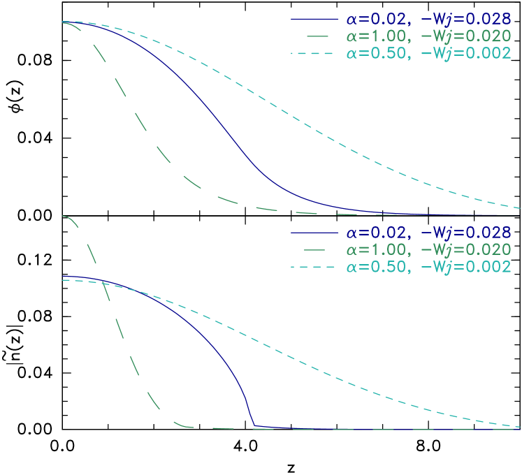
Figure 4: Potential and density deficit $z$-profiles (at $r=0$), illustrating different model parameter settings.

Different types of parallel ($z$) profiles are illustrated in Fig. 4. They are actually profiles at $r=0$ of fully self-consistent multidimensional solutions, whose attainment is the subject of the next section, but they are little different from the separable treatment of this section. When the power is very small, $\alpha=0.02$, the $\tilde{f}$ shape is essentially a waterbag (flat for $W<-W_{j}$, and zero for $W>W_{j}$) giving a density deficit $|\tilde{n}(z)|$ that is nearly elliptical. This case gives the steepest onset of deficit, and has a $\tilde{f}$-slope singularity, but at $W=W_{j}$, not the separatrix. The potential has only moderate curvature at $z=0$.

By contrast, when $\alpha=1$ the $\tilde{f}(W)$ is linear, without a slope singularity anywhere, but naturally tends to peak more near $z=0$, giving charge and potential profiles that are considerably narrower. The case $\alpha=0.5$ makes $|\tilde{n}|$ a linear function of $\phi$; and choosing a small $-W_{j}=0.002$ ($-W_{j}/\psi=0.02$) causes the profiles to extend to considerably larger $z$ than the other examples, even though the $\phi$-curvature at $z=0$ is almost the same as the waterbag case. A limitation of this power deficit model is that it cannot represent the non-monotonic $\tilde{f}(W)$ profiles required to give a flat region of $\phi(z)$ near $z=0$.

IV Relaxation to true non-separable equilibrium

In addition to providing analytic self-consistent solutions when potential gradients are ignorable or separable, the model potential is also suitable for calculating numerically the full non-separable potential form for two and three dimensional potential variation. Obviously, to produce a hole of finite transverse dimension one must have transverse (e.g. radial) variation of the peak potential $\psi$, which will imply for the present model radial variation of $\tilde{f}_{\psi}$ and $W_{j}$ (and possibly $\alpha$ but here we shall suppose $\alpha$ is uniform).

In principle it ought to be possible to construct self-consistent profiles for any specified distribution function of the form $\tilde{f}=\tilde{f}(W_{\parallel},r)$ which gives rise to charge-density $\rho(\phi,r)=1-n_{p}-n_{t}=1-n_{f}-\tilde{n}=1-n(\phi,r)$. When substituted into Poisson’s equation $-\nabla^{2}\phi=\rho(\phi,r)$, a well-posed problem arises with some boundary conditions. It is non-linear in general, of course, so typically will require numerical solution, although in regions where $\tilde{n}$ is zero, the Modified Helmholtz equation (Debye shielding) in multiple dimensions will be obtained when $n_{f}$ is linear in $\phi$.

Particle-in-cell (PIC) simulations have frequently observed multi-dimensional holes arising from initially uniform unstable plasma distributionsMottez et al. (1997); Miyake et al. (1998); Goldman, Oppenheim, and Newman (1999); Oppenheim, Newman, and Goldman (1999); Muschietti et al. (2000); Oppenheim et al. (2001); Singh, Loo, and Wells (2001); Lu et al. (2008). And isolated equilibria depending on non-uniform trapped distributions have been constructed and demonstrated to persist for extended time durations using a PIC code by the present author. But a PIC code uses more physics than just a knowledge of $n(\phi,r)$. It turns out that to find a multidimensional potential structure that is solitary (having boundary conditions only at infinity), based purely on $\rho(\phi)$, is in fact not a well posed problem. The work of Krasovsky, Matsumoto, and Omura (2004a) using the two-region piecewise linear-density variation $\rho(\phi)$ (as discussed above, with $\alpha=1/2$ but without any explicit dependence on $r$) purports to find a non-spherical equilibrium with a universal $\rho(\phi)$ dependence by prescribing a non-spherical contour shape of the join potential $\phi_{j}=-W_{j}$, solving the resulting Helmholtz equation for $\phi$ inside the contour as a sum of harmonics, and thereby prescribing the fixed $\tilde{n}(r,z)$. However, their presumption that this solution can be extended without discontinuity to the external region appears to be incorrect. In any case — and this is the key problem of any multidimensional solitary equilibrium — a $\rho(\phi)$ non-spherical equilibrium prescribed by a $\phi_{j}$ contour shape constraint is unstable to potential changes if the constraint is removed.

A numerical iterative relaxation on a suitable multidimensional mesh of a potential profile in accordance with $-\nabla^{2}\phi=\rho(\phi,r)$ demonstrates this instability. Explorations of such relaxation approaches have shown that schemes based upon iterations in which Poisson’s equation is solved for given $\rho$ followed by updating $\rho$ in accordance with prescribed $\rho(\phi,r)$ do not generally converge to electron holes. The potential either grows without limit in the large-$\phi$ region, or collapses to zero giving a null ($\phi=0$ everywhere) converged solution. And this behavior is independent of the degree of partial relaxation, because it is not merely numerical. The instability is physically intuitive, since $\rho$ is an increasing function of $\phi$ in the positive charge region, and positive $\rho$ generally gives rise to positive $\phi$ in Poisson’s equation, which amounts to positive feedback of a perturbation near the potential peak.

In one dimension, it is sometimes possible to stabilize relaxation iterations so as to converge to the desired equilibrium by using an implicit scheme, but this requires the iteration to start close enough to the final potential profile, otherwise either collapse or stochastic fluctuations result. Normally of course one-dimensional equilibria are obtained for specified $\rho(\phi)$ not by relaxation but by direct integration using the “classical” potential $V(\phi)=\int\rho d\phi$. Such an approach does not readily carry over to multi-dimensional problems, because the transverse field divergence contribution is known only when the potential profile is known. In multiple dimensions, even implicit relaxation schemes experience instability.

Physically steady, stable, solitary electron hole equilibria nevertheless exist. How? The answer is that their actual time-dependent electron dynamics is not represented by prescribing $\rho(\phi,r)$. The most important dynamic effect is probably that a time rate of change of the potential violates the conservation of total energy along particle orbits, thereby dynamically changing the form of $\rho(\phi,r)$ in response to a non-steady perturbation. A successful numerical relaxation scheme to find the equilibrium must represent some of that stabilizing physical dynamics. One way to represent the dynamics approximately is to regard the charge density as being specified as a function of the potential difference between the peak potential $\psi$ (at $z=0$) and the potential elsewhere ($z\not=0$) so that $\rho=\rho(\psi-\phi,r)$. This mocks up the idea that $\rho$ does not change in response to time-dependent evolution of $\phi$ at only a fixed point, but rather has non-local dynamic response contributions. Raising or lowering uniformly the entire potential profile does not then change $\rho(z)$.

I have implemented schemes that take just the trapped particle deficit $\tilde{f}$ to be a fixed function of $\psi-\phi$ (and $r$). The screening response, consisting of the passing particles at positive energy and flat trapped distribution $f_{f}$ at negative energy (which in total I call the flat-trap or reference distribution) remains, as before, a fixed function of $\phi$ (approximately $\propto\phi$). This amounts to supposing that the passing particle density plus the flat contribution in the trapped region responds quickly to changes in potential, while the trapped deficit does not. Heuristic justification is that passing particles are rapidly exchanged out of the hole and the flat trap level $f_{\infty}(0)$ does not depend on $\phi$. Screening is a stabilizing contribution, approximately the Boltzmann response. The power model of density deficit is used; so mathematically the density derived from eq. (14) is

$$\tilde{n}(\phi)=-{(\alpha+3/2)\over 2}{\psi_{d}^{2}(\phi-\psi+\psi_{d}+W_{jd})^{1/2+\alpha}\over(\psi_{d}+W_{jd})^{3/2+\alpha}}F_{\perp},$$ (15)

where $\psi_{d}$, $W_{jd}$, and $F_{\perp}$ (and $\alpha$) are fixed quantities expressing the desired (subscript $d$) $\psi$, $W_{j}$, initialized before the relaxation, and the $F_{\perp}$ value calculated from the $\psi_{d}$ profile $V_{\perp d}$ plus $V_{f}$. The $\phi$ and $\psi$ change with iteration, but by prescription $\tilde{n}$ depends only on their difference.

Two different algorithms for solving for the potential update have been investigated, one using an ad hoc implicit advance along alternating directions. The other (much faster) simply solves Poisson’s equation as a Modified Helmholtz equation in an $rz$-domain, given the difference from pure linear screening (the non-Helmholtz part of the charge density, $\Delta\rho$ using the prior $\phi$) as a source:

$$\nabla^{2}\phi-\phi/\lambda_{s}^{2}=-\Delta\rho=\tilde{n}+n_{f}-1-\phi/\lambda_{s}^{2},$$ (16)

where the screening length is taken as $\lambda_{s}=(dn_{f}/d\phi)^{-1/2}$ at $\phi\to 0$. The Helmholtz equation (16) is solved at each iteration using the cyclic reduction routine sepeli from the “Fishpack” library. Boundary conditions are $d\phi/dr=0$ at $r=0$, $d\phi/dz=0$ at $z=0$, $d\ln\phi/dr=-1/\lambda_{s}-1/r_{max}$ at $r=r_{max}$, and $d\ln\phi/dz=-1/\lambda_{s}$ at $z=z_{max}$. The distant boundaries do not matter much as long as they are far enough away. These two codes use in addition a simple Padé approximation for the fully nonlinear screening (flat-trap) response $n_{f}$ of an external Maxwellian of arbitrary drift velocity (not just the $n_{f}-1=\phi$ approximation). They thus accommodate any speed or depth of hole. The agreement between the two codes helps verify their coding.

IV.1 Global density functional yields only 1-D holes

One version of these relaxation calculations supposes that the potential difference $\psi-\phi$ on which the electron density deficit $\tilde{n}$ depends, is the quantity $\phi(0,0)-\phi(r,z)$. That is, the difference between the local potential and the potential at the origin, which is where the global peak in potential lies. This may be called the “global functional”. The other, called the “parallel functional”, is instead $\phi(r,0)-\phi(r,z)$; that is, the difference at fixed radial position between the local potential and the ridge at $z=0$ along the parallel coordinate $z$.

A summary of the results of the global functional model relaxation is simple. Electron hole equilibria are found, but they are spherically symmetric, no matter what the initial starting state is. Even highly elongated initial potential shapes rapidly relax to spherically symmetric equilibria that depend solely on the spherical radial distance from the origin $R=\sqrt{r^{2}+z^{2}}$. These are therefore one-dimensional, not multidimensional, though the one dimension is spherical radius not a cartesian coordinate.

IV.2 Radially varying density parallel functional gives 2-D holes

In this section we examine the two-dimensional (axisymmetric) holes obtained when the density deficit takes the form of the power model, eq. (15), in which $\psi=\phi(r,0)$, that is, the parallel functional model $\tilde{n}$. The profile $\psi_{d}(r)$ is effectively a free choice but the results shown will use the following parametrization whose monotonic shape is sufficiently versatile for present purposes:

$$\begin{split}&\psi_{d}(r)=\psi_{d0}{1+\exp(r_{t}/\lambda_{s})\over\cosh(r/\lambda_{s})+(1+Dr^{2})\exp(r_{t}/\lambda_{s})},\\ &W_{jd}(r)=W_{j0}\psi_{d}(r)/\psi_{d0}.\end{split}$$ (17)

Here the adjustable (uniform) parameter $r_{t}$, when positive, is approximately the radius of a flattened potential region for $r\lesssim r_{t}$; large negative $r_{t}$ removes all flattening, giving a ${\rm sech}(r/\lambda_{s})$ shape. Parameter $D$ is approximately half an extra negative curvature $-(1/\phi)d^{2}\phi/dr^{2}$ of the potential, modifying the top’s flatness if desired. The uniform screening length $\lambda_{s}$ is not considered to be adjustable, but depends on the passing particle distribution, notably its mean speed relative to the hole, or equivalently the hole speed. The form chosen for eq. (17) recognizes that at large $r$, where $\tilde{n}$ is negligible, the transverse potential variation (at $z=0$) is dominated by the screening length and asymptotes to $1/\cosh(r/\lambda_{s})\to\exp(-r/\lambda_{s})$. The join energy is taken to have a desired profile the same shape as $\psi_{d}$, giving a constant desired ratio $W_{jd}(r)/\psi_{d}(r)=W_{j0}/\psi_{d0}$, with values in the approximate range $-0.05$ to $-0.5$ being physically plausible for most $\alpha$ values. Recall that, for $W_{\parallel}>W_{j}$, the trapped distribution function is independent of energy, equal to $f_{0}(0)$, plausibly accommodating rapid trapping and detrapping of particles on stochastic orbits with energies above $W_{j}$.

Figure 5: Example prescribed desired radial profiles of peak potential $\psi$ and negative join energy $-W_{j}$ ($\alpha=1/2$, $r_{t}=5$, $D=0$).

Fig. 5 shows an example of the prescribed radial profiles of peak potential $\psi$ and negative join energy $-W_{j}$ (for $\alpha=1/2$, $r_{t}=5$, $D=0$).

The final fully self-consistent equilibrium found for this example (after 20 relaxation iterations) is shown in the contour plot of Fig. 6.

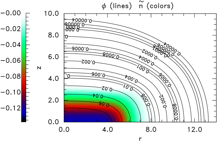
Figure 6: The final self-consistent hole solution based on the prescription of Fig. 5, showing logarithmically spaced contours of potential (lines) and the trapped-density deficit $\tilde{n}$ (colors) that sustains it.

The chosen $r_{t}$ prescribes a hole considerably extended in the transverse dimension. Beyond the region of non-zero electron density deficit $\tilde{n}$, the potential contours gradually become less oblate. The contours there show outward decay of potential that is approximately exponential ${1\over\phi}{\partial\phi\over\partial R}\sim const.$; the spacing of two adjacent contours is almost independent of angle in this $rz$-plane. At radial positions $r\gtrsim r_{t}$ the contour lines are nearly circular, concentric about $r\sim r_{t}$. Nearer the origin, the potential contours are still oblate, but it is evident that they do not follow lines of level density deficit $\tilde{n}$. For this equilibrium, therefore, the deficit charge density $\tilde{\rho}=-\tilde{n}$ is not a function just of $\phi$. It is a function also of $r$. As has already been observed in the previous section, such explicit $r$-dependence is essential to obtain multidimensional (non-spherical) holes. That $r$-dependence is implicitly prescribed by $\psi_{d}(r)$ and $W_{jd}(r)$. All these qualitative comments are observed to apply to essentially the full range of possible equilibria.

In Fig. 7 are shown profiles of several parameters along the radial axis ($z=0$). The solution potential $\psi(r)$ normalized to its peak at the origin ($\psi(0)$) proves to have a shape gratifyingly close to what was prescribed, $\psi_{d}(r)/\psi_{d}(0)$ (the dashed line).

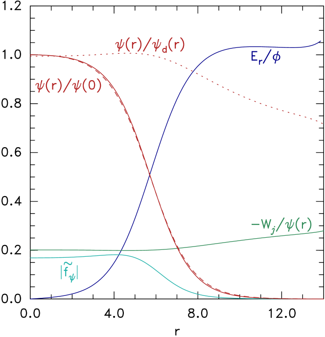
Figure 7: The radial shapes of the solved equilibrium parameters: potential $\psi(r)/\psi(0)$ with (dashed) its desired value $\psi_{d}(r)/\psi_{d}(0)$, and (dotted) their ratio, the peak distribution function deficit $|\tilde{f}_{\psi}|$, the ratio of join energy to potential peak $-W_{j}(r)/\psi(r)$, and the potential logarithmic gradient $E_{r}/\phi$ (at $z=0$).

A way of showing the absolute agreement out to large radii is the dotted line of $\psi(r)/\psi_{d}(r)$, which deviates significantly from unity only at radii far from the hole, where the potential is already small. The $z=0$ value of the distribution function deficit $|\tilde{f}_{\psi}|$, which is fixed by its derivation prior to relaxation from $\psi_{d}$ and $W_{jd}$, is slightly peaked off-axis (at $r>0$). The reason is that it takes into account the transverse electric field divergence $\nabla_{\perp}^{2}\phi$ of the prescribed potential, which requires an enhanced deficit in regions of negative $\psi$-curvature. The deficit $|\tilde{f}_{\psi}|$ falls quickly to zero at large radius where the potential profile is governed essentially by the screening effect of passing particles. If a potential that did not have exponential radial variation in this distant region had been prescribed, $|\tilde{f}_{\psi}|$ would not have become as quickly negligible as it does here. This exponential potential variation at distant $r$ is evident in the asymptotic approximately flat $E_{r}/\phi$ at a value of approximately 1. It is not exactly 1 because, although $\lambda_{s}$ is effectively 1, the solution of the Helmholtz equation is $\phi\propto{1\over r}\exp(-r/\lambda_{s})$ with an extra $1/r$ factor contributing a correction of order $\lambda_{s}/r$ to the slope. The fractional join energy $-W_{j}/\psi$ shows variation with radius that is the inverse of that of $\psi(r)/\psi_{d}(r)$ because the iteration scheme holds the potential difference $\psi-\phi_{j}=\psi_{d}-\phi_{jd}=\psi_{d}+W_{jd}$ fixed.

Fig. 8 shows at a range of $r$ positions (0, 2, 4, …) the relative parallel shape $\phi(z)/\psi$. For $r\lesssim r_{t}$ this shape is practically invariant. In this inner radial range the potential is in fact separable to a good approximation. And, as shown by the point markers plotted over the lines, the agreement with the analytic solution for $\alpha=1/2$ (equations 9 and 10) in this region is excellent.

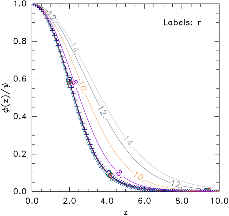
Figure 8: Parallel profiles of potential shape for a range of radial positions, showing the non-separable form of the solution. Marked points show the analytic power deficit model prescribed (‘+’ at $\phi_{d}>-W_{j}$ and ‘$\times$’ at $\phi_{d}<-W_{j}$), in good agreement at small radius.

At larger radii, however, the parallel extent of the potential profile increases, showing that in the wing an assumption of separability is inapplicable.

IV.3 Consequences for satellite observations

Since satellites encountering electron holes measure the components of the electric field, rather than the potential directly. It is helpful to derive from an equilibrium like Fig. 6 contours of the perpendicular and parallel electric field. These are shown in Fig. 9(a).

(a)MMM

(b)

Figure 9: (a) Contours of parallel and perpendicular electric field corresponding to the equilibrium of Fig. 6. (b) Peak values of field along constant $r$ and their ratio versus radial position.

Generally holes move predominantly in the parallel direction at a fraction of the electron thermal speed, which is usually much faster than satellites move. Therefore to a first approximation, the transit of an electron hole past a satelite corresponds to relative motion of the satellite along a vertical (fixed-$r$) line through the profile of the hole. The anticipated time dependence of electric field is the corresponding spatial dependence along such a line. As can easily be understood from the contours, such motion gives rise to bipolar $E_{\parallel}$ and simultaneously unipolar $E_{\perp}$ profiles. The occurrence of such features is often used to identify electron hole events. One simple and frequently used measure of electron hole amplitude is the peak absolute value of the electric field. For $E_{\perp}$ this usually occurs at $z=0$ the point of closest approach; but for $E_{\parallel}$ it is always at $|z|>0$. Fig. 9(b) therefore plots the peak values of $|E_{\perp}|$ and $|E_{\parallel}|$ along each line $r=const$ as a function of $r$.

The ratio of electric field peaks, $E_{\perp}/E_{\parallel}$, has often been used in past satellite data analysis as a proxy for the aspect ratio of an electron hole: that is, the ratio of the potential’s scale lengths in the parallel and perpendicular directions is supposed $L_{\perp}/L_{\parallel}\sim E_{\parallel}/E_{\perp}$. Fig. 9 is an important caution for this practice. The entire $r$-profile of this ratio comes from a single electron hole model equilibrium, in which the actual aspect ratio $L_{\perp}/L_{\parallel}$ of the density deficit is approximately 3 and the aspect ratio of the potential contours closer to 2. Nevertheless the model shows that the observed ratio $E_{\perp}/E_{\parallel}$ can, all depending on $r$, be anywhere between 0 and $\sim 5$. The most probable or mean value of the ratio to be observed, supposing that the nearest distance of approach is random, is determined by whatever selection criterion governs the distant cut-off of selection of events as electron hole encounters. If this cut-off is taken as sharp, corresponding to a specific radial distance (e.g. $r=c$), or value of field component relative to its peak (which would correspond to $r=c$), then the probability distribution of detected radii is $p(r)=r/\int_{0}^{c}rdr=2r/c^{2}$ whose maximum is at $r=c$ and whose mean is $r=2c/3$. The corresponding probability distribution of $E_{\perp}(r)/E_{\parallel}(r)=A(r)$ is

$$p(A)=p(r(A)){dr\over dA}={1\over c^{2}}{dr^{2}\over dA}.$$ (18)

The most probable value is $E_{\perp}/E_{\parallel}=A(c)$, and the mean depends on the shape of the ratio profile but if $A(r)$ is approximately parabolic it is $E_{\perp}/E_{\parallel}\sim A(c/2)$. If we suppose, for example, that the selection criterion gives $c=6$, then for the profile shown we find the peak electric field ratio is $\sim 1.8$ and the mean is $\sim 0.18$, while if $c=8$ these values become $\sim 3$ and $\sim 0.25$. Thus, the most probable field ratio gives naively an aspect ratio 4 to 6 times smaller than the actual hole scale-length $L_{\perp}/L_{\parallel}$ and the mean field ratio gives roughly twice the actual. This is a disappointingly large interpretational uncertainty. It reemphasizes the statistical importance of the hole detection algorithm, and the great value of obtaining multiple simultaneous satellite passages through an electron hole (such as can be obtained using MMSSteinvall et al. (2019); Lotekar et al. (2020)) for estimating the hole’s transverse extent without relying on the $E_{\perp}/E_{\parallel}$ ratio.

IV.4 Different radial shapes

The earlier Fig. 1 shown in the introduction is a different example that illustrates the versatility of the equilibrium prescription. The independent parameter adjustments make it more oblate but with a more peaked radial profile ($r_{t}=10$, $D=0.03$, $\alpha=1/2$), and greater amplitude ($\psi(0)=0.5$, $-W_{j}=0.1$). Fig. 10 shows the summary plots, in which the shape changes are evident.

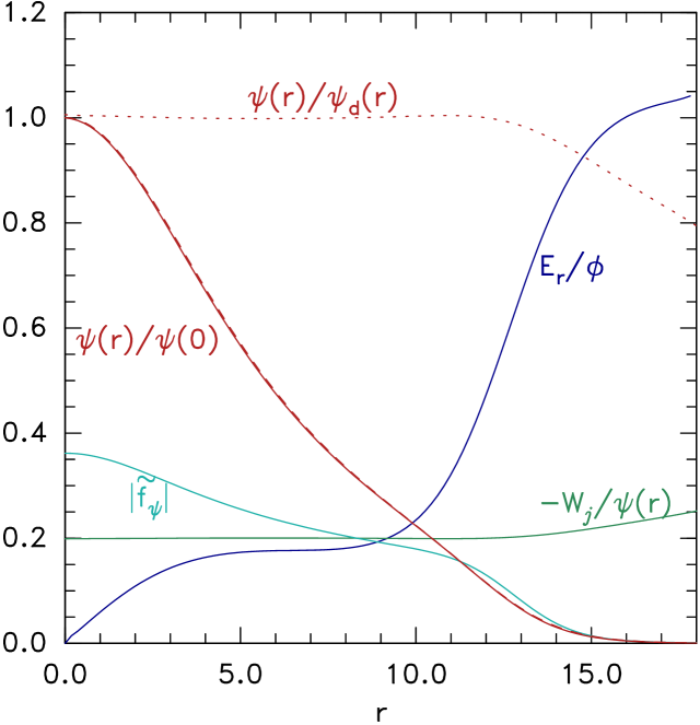
(a)MM

(b)

Figure 10: Equilibrium solution parameter radial profiles (a), and profiles of electric field peak values (b), for the hole illustrated in Fig. 1.

The peak potential $\psi(r)$, in Fig. 10(a), now has no flat top, but falls steadily out to a radius of approximately $r=12$ under control of the more peaked $\tilde{f}_{\psi}$ profile, giving a flatter $E_{r}$ profile. Then $\tilde{f}_{\psi}$ falls off rapidly into the exponential region of $\psi(r)$ where $E_{r}\over\phi$ rises to unity. Notice that the maximum value of $|\tilde{f}_{\psi}|\simeq 0.36$ is close to the maximum permissible (0.399), showing that this equilibrium requires the deeply trapped orbits to be almost completely depleted of electrons near the origin. The peak fields along fixed $r$, Fig. 10(b), show a more extended region of flat $E_{\perp}/E_{\parallel}$ before it rises in the exponential region. Still, even the flat region $E_{\perp}/E_{\parallel}\simeq 0.5$ does not agree very well with the typical inverse contour aspect ratio $L_{\parallel}/L_{\perp}\sim 1/3$. Despite the substantial radial gradients, the parallel potential relative shapes (not shown) do not significantly differ until $r\gtrsim 12$. They agree with the analytic form in approximately the same way as Fig. 8. Thus, they are approximately separable until a radius at which radial exponential decay sets in, like the previous equilibrium example.

V Conclusions

A technique for constructing fully self-consistent multidimensional electron hole equilibria in the drift limit of negligible gyro-radius has been described and illustrated. It starts from a versatile phase-space distribution deficit form that satisfies the plausibility constraint of being zero at and immediately below the parallel energy trapping threshold, and from a desired radial transverse potential variation. The analytic results of an approximation of separability of the potential are derived. Dropping the separable approximation, which cannot apply everywhere, requires an iterative relaxation to a fully self-consistent (non-separable) equilibrium. Such relaxation cannot be carried out under an assumption that the density deficit is a function only of potential, because that leads to instability. An alternative scheme, embodying numerically some aspects of the electron dynamic response, finds multidimensional equilibria. But it also shows that no stable non-spherical solitary equilibrium exists without there being explict dependence of density deficit on transverse position. The deviation of the full axisymmetric equilibria from the separable form proves to be remarkably small except in the profile wings. The resulting electric field component spatial dependencies, observable by satellites, are illustrated for different oblate hole shapes. They show that the ratio of peak perpendicular and parallel electric fields $E_{\perp}/E_{\parallel}$ is unfortunately a very uncertain measure of the aspect ratio $L_{\parallel}/L_{\perp}$ of the potential or charge distributions of electron holes. This conclusion re-emphasizes the importance of obtaining multiple simultaneous in-situ measurements such as can be obtained from multiple-satellite missions, in order to establish the true spatial structure of naturally occurring electron holes.

Supporting Data Statement

The code used to calculate the equilibria and plot the figures of this paper is open source and can be obtained from https://github.com/ihutch/helmhole.

References

- Matsumoto et al. (1994) H. Matsumoto, H. Kojima, T. Miyatake, Y. Omura, M. Okada, I. Nagano, and M. Tsutsui, “Electrostatic solitary waves (ESW) in the magnetotail: BEN wave forms observed by GEOTAIL,” Geophysical Research Letters 21, 2915–2918 (1994).
- Ergun et al. (1998) R. E. Ergun, C. W. Carlson, J. P. McFadden, F. S. Mozer, L. Muschietti, I. Roth, and R. J. Strangeway, “Debye-Scale Plasma Structures Associated with Magnetic-Field-Aligned Electric Fields,” Physical Review Letters 81, 826–829 (1998).
- Bale et al. (1998) S. D. Bale, P. J. Kellogg, D. E. Larsen, R. P. Lin, K. Goetz, and R. P. Lepping, “Bipolar electrostatic structures in the shock transition region: Evidence of electron phase space holes,” Geophysical Research Letters 25, 2929–2932 (1998).
- Mangeney et al. (1999) A. Mangeney, C. Salem, C. Lacombe, J.-L. Bougeret, C. Perche, R. Manning, P. J. Kellogg, K. Goetz, S. J. Monson, and J.-M. Bosqued, “WIND observations of coherent electrostatic waves in the solar wind,” Annales Geophysicae 17, 307–320 (1999).
- Pickett et al. (2008) J. S. Pickett, L.-J. Chen, R. L. Mutel, I. W. Christopher, O. Santolı´k, G. S. Lakhina, S. V. Singh, R. V. Reddy, D. A. Gurnett, B. T. Tsurutani, E. Lucek, and B. Lavraud, “Furthering our understanding of electrostatic solitary waves through Cluster multispacecraft observations and theory,” Advances in Space Research 41, 1666–1676 (2008).
- Andersson et al. (2009) L. Andersson, R. E. Ergun, J. Tao, A. Roux, O. Lecontel, V. Angelopoulos, J. Bonnell, J. P. McFadden, D. E. Larson, S. Eriksson, T. Johansson, C. M. Cully, D. N. Newman, M. V. Goldman, K. H. Glassmeier, and W. Baumjohann, “New features of electron phase space holes observed by the THEMIS mission,” Physical Review Letters 102, 225004 (2009).
- Wilson et al. (2010) L. B. Wilson, C. A. Cattell, P. J. Kellogg, K. Goetz, K. Kersten, J. C. Kasper, A. Szabo, and M. Wilber, “Large-amplitude electrostatic waves observed at a supercritical interplanetary shock,” Journal of Geophysical Research: Space Physics 115, A12104 (2010).
- Malaspina et al. (2013) D. M. Malaspina, D. L. Newman, L. B. Willson, K. Goetz, P. J. Kellogg, and K. Kerstin, “Electrostatic solitary waves in the solar wind: Evidence for instability at solar wind current sheets,” Journal of Geophysical Research: Space Physics 118, 591–599 (2013).
- Malaspina et al. (2014) D. M. Malaspina, L. Andersson, R. E. Ergun, J. R. Wygant, J. W. Bonnell, C. Kletzing, G. D. Reeves, R. M. Skoug, and B. A. Larsen, “Nonlinear electric field structures in the inner magnetosphere,” Geophysical Research Letters 41, 5693–5701 (2014).
- Vasko et al. (2015) I. Y. Vasko, O. V. Agapitov, F. Mozer, A. V. Artemyev, and D. Jovanovic, “Magnetic field depression within electron holes,” Geophysical Research Letters 42, 2123–2129 (2015).
- Mozer et al. (2016) F. S. Mozer, O. A. Agapitov, A. Artemyev, J. L. Burch, R. E. Ergun, B. L. Giles, D. Mourenas, R. B. Torbert, T. D. Phan, and I. Vasko, “Magnetospheric Multiscale Satellite Observations of Parallel Electron Acceleration in Magnetic Field Reconnection by Fermi Reflection from Time Domain Structures,” Physical Review Letters 116, 4–8 (2016), arXiv:arXiv:1011.1669v3 .
- Hutchinson and Malaspina (2018) I. H. Hutchinson and D. M. Malaspina, “Prediction and Observation of Electron Instabilities and Phase Space Holes Concentrated in the Lunar Plasma Wake,” Geophysical Research Letters 45, 3838–3845 (2018).
- Mozer et al. (2018) F. S. Mozer, O. V. Agapitov, B. Giles, and I. Vasko, “Direct Observation of Electron Distributions inside Millisecond Duration Electron Holes,” Physical Review Letters 121, 135102 (2018).
- Hutchinson (2020) I. H. Hutchinson, “Particle trapping in axisymmetric electron holes,” Journal of Geophysical Research: Space Physics 125 (2020), 10.1029/2020JA028093, e2020JA028093 10.1029/2020JA028093, https://agupubs.onlinelibrary.wiley.com/doi/pdf/10.1029/2020JA028093 .
- Hutchinson (2021) I. H. Hutchinson, “Oblate electron holes are not attributable to anisotropic shielding,” Physics of Plasmas (2021), accepted for publication.
- Bernstein, Greene, and Kruskal (1957) I. B. Bernstein, J. M. Greene, and M. D. Kruskal, “Exact nonlinear plasma oscillations,” Physical Review 108, 546–550 (1957).
- Turikov (1984) V. A. Turikov, “Electron Phase Space Holes as Localized BGK Solutions,” Physica Scripta 30, 73–77 (1984).
- Schamel (1986) H. Schamel, “Electrostatic Phase Space Structures in Theory and Experiment,” Physics Reports 140, 161–191 (1986).
- Eliasson and Shukla (2006) B. Eliasson and P. K. Shukla, “Formation and dynamics of coherent structures involving phase-space vortices in plasmas,” Physics Reports 422, 225–290 (2006).
- Hutchinson (2017) I. H. Hutchinson, “Electron holes in phase space: What they are and why they matter,” Physics of Plasmas 24, 055601 (2017).
- Chen and Parks (2002) L.-J. Chen and G. K. Parks, “BGK electron solitary waves in 3D magnetized plasma,” Geophysical Research Letters 29, 41–45 (2002).
- Schamel (1979) H. Schamel, “Theory of Electron Holes,” Physica Scripta 20, 336–342 (1979).
- Chen, Thouless, and Tang (2004) L.-J. Chen, D. Thouless, and J.-M. Tang, “Bernstein–Greene–Kruskal solitary waves in three-dimensional magnetized plasma,” Physical Review E 69, 55401 (2004).
- Muschietti et al. (2002) L. Muschietti, I. Roth, C. W. Carlson, and M. Berthomier, “Modeling stretched solitary waves along magnetic field lines,” Nonlinear Processes in Geophysics 9, 101–109 (2002).
- Jovanović et al. (2002) D. Jovanović, P. K. Shukla, L. Stenflo, and F. Pegoraro, “Nonlinear model for electron phase-space holes in magnetized space plasmas,” Journal of Geophysical Research: Space Physics 107, 1–6 (2002).