Representation of Context-Specific Causal Models with Observational and Interventional Data

Abstract.

We consider the problem of representing causal models that encode context-specific information for discrete data using a proper subclass of staged tree models which we call CStrees. We show that the context-specific information encoded by a CStree can be equivalently expressed via a collection of DAGs. As not all staged tree models admit this property, CStrees are a subclass that provides a transparent, intuitive and compact representation of context-specific causal information. We prove that CStrees admit a global Markov property which yields a graphical criterion for model equivalence generalizing that of Verma and Pearl for DAG models. These results extend to the general interventional model setting, making CStrees the first family of context-specific models admitting a characterization of interventional model equivalence.

We also provide a closed-form formula for the maximum likelihood estimator of a CStree and use it to show that the Bayesian information criterion is a locally consistent score function for this model class.

The performance of CStrees is analyzed on both simulated and real data, where we see that modeling with CStrees instead of general staged trees does not result in a significant loss of predictive accuracy, while affording DAG representations of context-specific causal information.

1. Introduction

In this paper we introduce CStrees and interventional CStrees to represent context-specific conditional independence relations among discrete random variables in directed acyclic graph (DAG) models and their interventional extensions.

1.1. CStrees

In a DAG model, the nodes of the graph correspond to random variables and the non-edges encode conditional independence (CI) relations that the data-generating distribution must entail. For instance, any joint distribution for the vector of random variables $(X_{1},\ldots,X_{p})$ in the model defined by a DAG $\mathcal{G}=([p],E)$ satisfies the ordered Markov property which states that for some linear ordering $\pi=\pi_{1}\cdots\pi_{p}$ of the vertices $[p]$ that respects the directions of all arrows in $\mathcal{G}$, each node $X_{\pi_{i}}$ is independent of all of preceding variables $X_{\{\pi_{1},\ldots,\pi_{i-1}\}\setminus\mathop{\rm pa}\nolimits_{\mathcal{G}}(i)}$ given its direct causes $X_{\mathop{\rm pa}\nolimits_{\mathcal{G}}(i)}$; i.e., $X_{\pi_{i}}\mathchoice{\mathrel{\hbox to0.0pt{$\displaystyle\perp$\hss}\mkern 2.0mu{\displaystyle\perp}}}{\mathrel{\hbox to0.0pt{$\textstyle\perp$\hss}\mkern 2.0mu{\textstyle\perp}}}{\mathrel{\hbox to0.0pt{$\scriptstyle\perp$\hss}\mkern 2.0mu{\scriptstyle\perp}}}{\mathrel{\hbox to0.0pt{$\scriptscriptstyle\perp$\hss}\mkern 2.0mu{\scriptscriptstyle\perp}}}X_{\{\pi_{1},\ldots,\pi_{i-1}\}\setminus\mathop{\rm pa}\nolimits_{\mathcal{G}}(i)}\mid X_{\mathop{\rm pa}\nolimits_{\mathcal{G}}(i)}$. An intrinsic property of conditional independence statements of this form is that the independence of the two sets of variables $X_{\pi_{i}}$ and $X_{\{\pi_{1},\ldots,\pi_{i-1}\}\setminus\mathop{\rm pa}\nolimits_{\mathcal{G}}(i)}$ holds for any realization of the variables in the conditioning set $X_{\mathop{\rm pa}\nolimits_{\mathcal{G}}(i)}$. This feature of DAG models makes it infeasible to use them to encode distributions that satisfy context-specific conditional independence (CSI) relations; that is, conditional independence relations that hold only for a possibly strict subset of the realizations of the conditioning variables.

The problem of encoding additional CSI relations for distributions that belong to DAG models has been studied by several authors. These include the use of conditional probability tables (CPTs) with extra regularity structure (Boutilier et al., 1996), Bayesian multinets (Geiger and Heckerman, 1996), similarity networks (Heckerman, 1990) and chain event graphs (CEGs) (Smith and Anderson, 2008). Each of these proposed models has their individual strengths: CEGs admit a high level of expressiveness of context-specific information that comes at the cost of representations from which it is more difficult to extract causal information. On the other hand, Bayesian multinets are highly readable but limit their expressiveness to modeling how context-specific information impacts selected hypothesis variables. The contribution of CStrees is a family of causal models with the readability of a Bayesian multinet but with the ability to capture much more diverse CSI relations, similar to a CEG. CStrees are such that they admit a global Markov property and graphical characterization of model equivalence directly generalizing that of DAGs. These properties conveniently extend to interventional models, making CStrees the first family of context-specific causal models with a known graphical criterion for interventional model equivalence.

(a) A CStree $\mathcal{T}$.

(b) A CEG for $\mathcal{T}$.

(c) The sequence of context graphs $\mathcal{G}_{\mathcal{T}}$ for $\mathcal{T}$.

Figure 1. A CStree $\mathcal{T}$ on variables $X_{1},X_{2},X_{3},X_{4}$, where $X_{i}$ has outcomes $\{x_{i}^{1},x_{i}^{2}\}$. The same model can also be represented with the sequence of DAGs in (c).

As an example, consider the staged tree in Figure 1(a) and its CEG representation in Figure 1(b). From these two figures it might be difficult to read cause-effect relationships among variables as compared to a DAG, in which such information is encoded by a single directed edge between two nodes. Fortunately, the staged tree in Figure 1(a) is also a CStree. This means that the same model can be represented with the sequence of DAGs in Figure 1(c), where the direct cause-effect relations in each context are evident. This representation is similar to a Bayesian multinet or similiarity network but strictly more general in regards to the contexts in which causal information can be encoded. It is also worth noting that any distribution faithful to the tree in Figure 1(a) is only Markov to a complete DAG on four nodes. Hence, the alternative representation in Figure 1(c) is more expressive than a DAG while more transparent (i.e., easily read) than a staged tree or CEG.

Our point of departure is the theory of staged tree models, where CStrees admit a simple definition. After presenting the necessary background on staged trees, DAG models and CSI relations in Section 2, we devote Section 3 to establishing the main properties of CStrees. We show in Theorem 2.1 that a CStree model is equivalently represented by a collection of DAGs. Aside from this representation being more concise and readable, it can also be used to characterize CStrees that encode the same set of CSI relations (see Theorem 3.3). In particular, Corollary 3.6 characterizes equivalence of CStree models in terms of the skeletons and v-structures of their associated DAGs.

We conclude Section 3 by deriving a closed-form formula for the maximum likelihood estimator of a CStree (Proposition 3.7), and showing that the BIC is a locally consistent scoring criterion for CStrees (Proposition 3.8). We also give a brief discussion on the enumerative properties of CStrees.

1.2. Interventional CStrees

It is well-known that two different DAGs can encode the same set of conditional independence statements implied by their, respective, ordered Markov properties. With CStrees the same situation can occur, i.e., two different sets of context DAGs can encode the same CSI relations. Hence, the rudimentary causal information given via CI or CSI relations in the ordered Markov property is not enough to determine the directions of all direct cause-effect relations. A typical way of deciding on the direction of arrows that reverse between different, but equivalent, DAGs is to use additional data drawn from interventional distributions (Hauser and Bühlmann, 2012; Wang et al., 2017; Yang et al., 2018). Using a combination of observational and interventional distributions it is possible to refine an equivalence class of DAGs into smaller, interventional equivalence classes (Yang et al., 2018). Motivated by these developments, we introduce interventional CStrees and show that they behave in a similar fashion to interventional DAG models. This helps to refine the equivalence classes of CStrees by using interventions and it allows for the representation of more general context-specific interventional experiments.

Building on the characterization of equivalence for CStrees provided in Section 3, we consider context-specific, general interventions in CStrees in Section 4. We define interventional CStree models and formulate a context-specific $\mathcal{I}$-Markov property (see Definition 4.2) that generalizes the $\mathcal{I}$-Markov property for DAGs studied in (Yang et al., 2018). Via this generalization, we extend the characterization of interventional equivalence of DAGs given in (Yang et al., 2018) to a characterization of equivalence of interventional CStree models. To the best of the authors’ knowledge, this makes CStrees the first family of context-specific interventional models admitting a characterization of model equivalence. These results are based on the theory of general interventions in staged tree models studied in (Duarte and Solus, 2020) as it applies to the class of CStrees. In Sections 5 and 6 we apply these results to simulated and real data sets.

The proofs of all lemmas, theorems as well as supplementary material related to selected topics can be found in the appendices.

2. Preliminaries

In this section we introduce the necessary notation, definitions and theorems for staged tree models, discrete DAG models and context-specific conditional independence relations. For any positive integer $m$, set $[m]:=\{1,\ldots,m\}$. Let $X_{[p]}:=(X_{1},\ldots,X_{p})$ be a vector of discrete random variables where $X_{i}$ has state space $[d_{i}]$. The set $\mathcal{R}:=\prod_{i\in[p]}[d_{i}]$ is the state space of $X_{[p]}$, and its elements are denoted by $x_{1}\cdots x_{p}$, $(x_{1},\ldots,x_{p})$ or simply by $\mathbf{x}$. When it is important to distinguish the variable and the outcome of the variable, we will represent element $j\in[d_{i}]$ by $x_{i}^{j}$. Given $S\subset[p]$, we let $X_{S}:=(X_{i}:i\in S)$ be the subvector of $X_{[p]}$ indexed by the elements in $S$. The outcome space of $X_{S}$ is $\mathcal{R}_{S}:=\prod_{i\in S}[d_{i}]$ and its elements are denoted by $\mathbf{x}_{S}$. Given two disjoint subsets $S,T\in[p]$, we let the concatenation of strings $\mathbf{x}_{S}\mathbf{x}_{T}$ or of vectors $(\mathbf{x}_{S},\mathbf{x}_{T})$ denote the corresponding realization of $X_{S\cup T}$.

Let $\mathbb{R}^{|\mathcal{R}|}$ denote the real Euclidean space with one standard basis vector $e_{\mathbf{x}}$ for each outcome $\mathbf{x}\in\mathcal{R}$. The probability density function $f$ for a positive distribution over $X_{[p]}$ can be realized as the point $(f(\mathbf{x}):\mathbf{x}\in\mathcal{R})$ in the (open) probability simplex

$$\Delta_{|\mathcal{R}|-1}^{\circ}:=\left\{(f_{\mathbf{x}}:\mathbf{x}\in\mathcal{R})\in\mathbb{R}^{|\mathcal{R}|}:f_{\mathbf{x}}>0\mbox{ for all }\mathbf{x}\in\mathcal{R}\mbox{ and }\sum_{\mathbf{x}\in\mathcal{R}}f_{\mathbf{x}}=1\right\}.$$

A statistical model of positive distributions with realization space $\mathcal{R}$ is a subset of $\Delta_{|\mathcal{R}|-1}^{\circ}$.

2.1. Staged tree models

The class of staged tree models was first introduced in (Smith and Anderson, 2008), we refer the reader to (Collazo et al., 2018) for a detailed introduction to this model class.

A rooted tree $\mathcal{T}=(V,E)$ is a directed graph whose skeleton is a tree and for which there exists a unique node $r$, called the root of $\mathcal{T}$, whose set of parents $\mathop{\rm pa}\nolimits_{\mathcal{T}}(r):=\{k\in V:k\rightarrow r\in E\}$ is empty. For $v\in V$, let $\lambda(v)$ denote the unique directed path from $r$ to $v$ in $\mathcal{T}$. We also let $E(v):=\{v\rightarrow w\in E:w\in\mathop{\rm ch}\nolimits_{\mathcal{T}}(v)\},$ where $\mathop{\rm ch}\nolimits_{\mathcal{T}}(v):=\{k\in V:v\rightarrow k\in E\}$ is the set of children of $v$.

Definition 2.1.

Let $\mathcal{T}=(V,E)$ be a rooted tree, $\mathcal{L}$ a finite set of labels, and $\theta:E\rightarrow\mathcal{L}$ a labeling of the edges $E$. The pair $(\mathcal{T},\theta)$ is a staged tree if

1. $|\theta(E(v))|=|E(v)|$ for all $v\in V$, and

2. for any two $v,w\in V$, $\theta(E(v))$ and $\theta(E(w))$ are either equal or disjoint.

When the labeling $\theta$ is understood from context, we simply refer to $\mathcal{T}$ as a staged tree. The vertices of a staged tree are partitioned into disjoint sets called stages such that $v,w\in V$ are in the same stage if and only if $\theta(E(v))=\theta(E(w))$. The partition of $V$ into its stages is called a staging of $\mathcal{T}$. When we depict a staged tree, such as in Figure 1(a), we will color two nodes the same color to indicate that they are in the same stage, with the convention that any white nodes are in a stage with cardinality one.

The space of canonical parameters of a staged tree $\mathcal{T}$ is the set

$$\Theta_{\mathcal{T}}:=\left\{x\in\mathbb{R}^{|\mathcal{L}|}:\forall e\in E,x_{\theta(e)}\in(0,1)\text{ and }\forall v\in V,\sum_{e\in E(v)}x_{\theta(e)}=1\right\}.$$

Definition 2.2.

Let ${\bf i}_{\mathcal{T}}$ be the collection of all leaves of $\mathcal{T}$. The staged tree model $\mathcal{M}_{(\mathcal{T},\theta)}$ for $(\mathcal{T},\theta)$ is the image of the map $\psi_{\mathcal{T}}:\Theta_{\mathcal{T}}\longrightarrow\Delta^{\circ}_{|{\bf i}_{\mathcal{T}}|-1}$ where

$$\begin{split}\psi_{\mathcal{T}}&:x\longmapsto f:=\left(\prod_{e\in E(\lambda(v))}x_{\theta(e)}\right)_{v\in{\bf i}_{\mathcal{T}}}.\end{split}$$

We say that $f\in\Delta_{|{\bf i}_{\mathcal{T}}|-1}^{\circ}$ factorizes according to $\mathcal{T}$ if $f\in\mathcal{M}_{(\mathcal{T},\theta)}$. Two staged trees $\mathcal{T}$ and $\mathcal{T}^{\prime}$ are called statistically equivalent if $\mathcal{M}_{(\mathcal{T},\theta)}=\mathcal{M}_{(\mathcal{T}^{\prime},\theta^{\prime})}$.

Throughout this paper we work with trees that represent the outcome space of the vector of discrete random variables $X_{[p]}$ as a sequence of events. Given an ordering $\pi_{1}\cdots\pi_{p}$ of $[p]$, we construct a rooted tree $\mathcal{T}=(V,E)$ where $V:=\{r\}\cup\bigcup_{j\in[p]}\mathcal{R}_{\{\pi_{1},\ldots,\pi_{j}\}}$, and

$$E:=\{r\!\rightarrow\!x_{\pi_{1}}\!:\!x_{\pi_{1}}\!\in\![d_{\pi_{1}}]\}\cup\{x_{\pi_{1}}\cdots x_{\pi_{k-1}}\!\rightarrow\!x_{\pi_{1}}\cdots x_{\pi_{k}}:x_{\pi_{1}}\cdots x_{\pi_{k}}\in\mathcal{R}_{\{\pi_{1},\ldots,\pi_{k}\}},\!k\in\![p-1]\}.$$

The level of a node $v\in V$ is the number of edges in $\lambda(v)$, and for $k\in\{0,\ldots,p\}$, the $k^{th}$ level of $\mathcal{T}$, denoted $L_{k}$, is the collection of all nodes $v\in V$ with level $k$. Note that $L_{0}=\{r\}$, so we usually ignore this level when referring to the levels of $\mathcal{T}$. For the trees defined above and $k>0$, the $k^{th}$ level of $\mathcal{T}$ is $L_{k}=\mathcal{R}_{\{\pi_{1},\ldots,\pi_{k}\}}$. Hence, we associate the variable $X_{\pi_{k}}$ with level $L_{k}$ and denote this association by $(L_{1},\ldots,L_{p})\sim(X_{\pi_{1}},\ldots,X_{\pi_{p}})$. Given such a tree $\mathcal{T}$ with levels $(L_{1},\ldots,L_{p})\sim(X_{\pi_{1}},\ldots,X_{\pi_{p}})$, we call the ordering $\pi=\pi_{1}\cdots\pi_{p}$ the causal ordering of $\mathcal{T}$. These trees are also uniform; meaning that $|E(v)|=|E(w)|$ for any $v,w\in L_{k}$, for all $k\geq 0$. A staged tree is stratified if all its leaves have the same level and if any two nodes in the same stage are also in the same level.

For a uniform and stratified staged tree model $\mathcal{M}_{(\mathcal{T},\theta)}$, the parameter values on the edges $E(v)$ for $v\in\mathcal{R}$ abide by the chain rule (see (Duarte and Solus, 2020, Lemma 2.1)). Namely, if $f\in\mathcal{M}_{(\mathcal{T},\theta)}$ then for any $v=x_{\pi_{1}}\cdots x_{\pi_{p}}\in\mathcal{R}$ and $e=x_{\pi_{1}}\cdots x_{\pi_{k-1}}\rightarrow x_{\pi_{1}}\cdots x_{\pi_{k}}$ in $\lambda(v)$, it holds that $x_{\theta(e)}=f(x_{\pi_{k}}\mid x_{\pi_{1}}\cdots x_{\pi_{k-1}})$. A uniform, stratified staged tree $\mathcal{T}$ with levels $(L_{1},\ldots,L_{p})\sim(X_{\pi_{1}},\ldots,X_{\pi_{p}})$ is called compatibly labeled if

$$\theta(x_{\pi_{1}}\cdots x_{\pi_{k-1}}\rightarrow x_{\pi_{1}}\cdots x_{\pi_{k-1}}x_{\pi_{k}})=\theta(y_{\pi_{1}}\cdots y_{\pi_{k-1}}\rightarrow y_{\pi_{1}}\cdots y_{\pi_{k-1}}x_{\pi_{k}})$$

for all $x_{\pi_{k}}\in[d_{\pi_{k}}]$ whenever $x_{\pi_{1}}\cdots x_{\pi_{k-1}}$ and $y_{\pi_{1}}\cdots y_{\pi_{k-1}}$ are in the same stage. This condition ensures that edges emanating from $x_{\pi_{1}}\cdots x_{\pi_{k-1}}$ and $y_{\pi_{1}}\cdots y_{\pi_{k-1}}$ with endpoints corresponding to the same outcome $x_{\pi_{k}}$ of the next variable encode the invariance of conditional probabilities:

$$f(x_{\pi_{k}}\mid x_{\pi_{1}}\cdots x_{\pi_{k-1}})=f(x_{\pi_{k}}\mid y_{\pi_{1}}\cdots y_{\pi_{k-1}}).$$

2.2. DAG models

An important subclass of compatibly labeled staged trees are DAG models, which can alternatively be represented via a directed acyclic graph (DAG) (Smith and Anderson, 2008). Let $\mathcal{G}=([p],E)$ be a DAG on node set $[p]$ with set of directed edges $E$.

A joint distribution, or its density function $f$, over the vector $X_{[p]}$ is Markov to $\mathcal{G}$ if $f$ satisfies the recursive factorization property:

$$f(X_{1},\ldots,X_{p})=\prod_{i\in[p]}f(X_{i}\mid X_{\mathop{\rm pa}\nolimits_{\mathcal{G}}(i)}).$$ (1)

Let $\mathcal{M}(\mathcal{G})$ denote the collection of all densities that are Markov to $\mathcal{G}$. As noted earlier, we consider $\mathcal{M}(\mathcal{G})$ as a subset of $\Delta_{|\mathcal{R}|-1}^{\circ}$. A distribution (or $f$) satisfies the global Markov property with respect to $\mathcal{G}$ if, given disjoint $A,B,C\subset[p]$ with $A,B\neq\emptyset$, it entails the CI relation $X_{A}\mathchoice{\mathrel{\hbox to0.0pt{$\displaystyle\perp$\hss}\mkern 2.0mu{\displaystyle\perp}}}{\mathrel{\hbox to0.0pt{$\textstyle\perp$\hss}\mkern 2.0mu{\textstyle\perp}}}{\mathrel{\hbox to0.0pt{$\scriptstyle\perp$\hss}\mkern 2.0mu{\scriptstyle\perp}}}{\mathrel{\hbox to0.0pt{$\scriptscriptstyle\perp$\hss}\mkern 2.0mu{\scriptscriptstyle\perp}}}X_{B}\mid X_{C}$ whenever $A$ and $B$ are d-separated in $\mathcal{G}$ given $C$. The notion of d-separation is defined in (Pearl, 2000). The following theorem states the model $\mathcal{M}(\mathcal{G})$ is in fact a conditional independence model determined by the CI relations encoded via d-separation in the DAG $\mathcal{G}$.

Theorem 2.1.

A distribution $f\in\Delta_{|\mathcal{R}|-1}^{\circ}$ is Markov to a DAG $\mathcal{G}$ if and only if it satisfies the global Markov property with respect to $\mathcal{G}$.

It is possible that two different DAGs encode the exact same set of conditional independence relations via the global Markov properties, and hence represent the same model. In this case, the DAGs are Markov equivalent and we say that they belong to the same Markov equivalence class. There are multiple graphical characterizations of Markov equivalence (Andersson and Perlman, 1997; Chickering, 1995; Verma and Pearl, 1990a).

Theorem 2.2 (Verma and Pearl (1990a)).

Two DAGs $\mathcal{G}$ and $\mathcal{H}$ are Markov equivalent if and only if they have the same skeleton and v-structures.

The skeleton of a DAG refers to its underlying, undirected graph, and a v-structure refers to any pair of edges in the DAG $i\rightarrow k$ and $k\leftarrow j$ for which there is no edge between $i$ and $j$ in the DAG. All discrete DAG models are also staged tree models (Smith and Anderson, 2008). A general construction for representing a DAG model with a staged tree is given in (Duarte and Solus, 2020, Example 3.2) as well as in (Smith and Anderson, 2008). We let $\mathcal{T}_{\mathbb{G}}$ denote the collection of all staged trees representing a DAG model.

Let $A,B,C,$ and $S$ be disjoint subsets of $[p]$. We say that $A$ and $B$ are contextually independent given $S$ in the context $X_{C}=\mathbf{x}_{C}$ if

$$f(\mathbf{x}_{A}\mid\mathbf{x}_{B},\mathbf{x}_{C},\mathbf{x}_{S})=f(\mathbf{x}_{A}\mid\mathbf{x}_{C},\mathbf{x}_{S})$$

holds for all $(\mathbf{x}_{A},\mathbf{x}_{B},\mathbf{x}_{S})\in\mathcal{R}_{A}\times\mathcal{R}_{B}\times\mathcal{R}_{S}$ whenever $f(\mathbf{x}_{A},\mathbf{x}_{B},\mathbf{x}_{S})>0$. We call this a context-specific conditional independence relation, or CSI relation, denoted $X_{A}\mathchoice{\mathrel{\hbox to0.0pt{$\displaystyle\perp$\hss}\mkern 2.0mu{\displaystyle\perp}}}{\mathrel{\hbox to0.0pt{$\textstyle\perp$\hss}\mkern 2.0mu{\textstyle\perp}}}{\mathrel{\hbox to0.0pt{$\scriptstyle\perp$\hss}\mkern 2.0mu{\scriptstyle\perp}}}{\mathrel{\hbox to0.0pt{$\scriptscriptstyle\perp$\hss}\mkern 2.0mu{\scriptscriptstyle\perp}}}X_{B}\mid X_{S},X_{C}=\mathbf{x}_{C}$.

A number of approaches have been proposed in an effort to account for CSI relations via DAG models. In addition to the Bayesian multinets, similarity networks and CEGs mentioned in the introduction, (Boutilier et al., 1996; Poole and Zhang, 2003) developed methods for representing the conditional probability tables (CPTs) for a DAG model by including CSI relations so as to speed-up computations for probabilistic inference. In (Chickering et al., 1997; Friedman and Goldszmidt, 1996), the authors utilized these methods to develop algorithms for learning a DAG model that is more representative of the context-specific independencies in the data-generating distribution.

3. CStrees

Staged tree models can encode a wide range of CSI relations. However, since the staged tree model representation depends on an underlying event tree that encodes the outcomes in the model, the complexity of this representation can increase rapidly leading to an exponential blow-up of the number of parameters. In response to this, Smith and Anderson (2008) introduced the chain event graph (CEG) associated to a staged tree model.

The CEG is a useful graphical summary of the different possible sequences of events that happen in the staged tree. Although the CEG is a simpler representation, its complexity is also directly dependent on the total number of possible unfoldings of events that occur in the model. As illustrated in Figure 1(b), it can still be challenging to read causal information directly from a CEG, even for very few variables.

In this section we define CStree models and show that they admit an alternative representation as a collection of context DAGs. The representation of a CStree via context DAGs has two advantages over its CEG representation: First, even if the number of outcomes in the model increases, the context DAG representation can still be very compact. Second, using context DAGs to encode the model assumptions allows the practitioner to transparently represent the direct causes of a variable in different contexts, whereas such information is typically harder to decipher from a CEG. Thus, restricting the class of staged tree models to CStrees increases the interpretability of the model without drastically increasing the complexity of the representation. Moreover, the class of CStrees admits a new criterion of model equivalence that does not hold for general staged trees and which is a direct generalization of Theorem 2.2.

3.1. Definition of CStrees

There are two defining conditions that distinguish CStrees from general staged trees: (1) the underlying event tree of a CStree always represents the outcome space of a vector of discrete random variables, and (2) the possible stagings of a CStree are more restrictive than in a general staged tree.

Definition 3.1.

Let $\mathcal{T}=(V,E)$ be a compatibly labeled staged tree with levels $(L_{1},\ldots,L_{p})\sim(X_{1},\ldots,X_{p})$. We say that $\mathcal{T}$ is a CStree if for every stage $S_{i}\subset L_{k-1}$, there exists $C_{i}\subset[k-1]$ and $\mathbf{x}_{C_{i}}\in\mathcal{R}_{C_{i}}$ such that

$$S_{i}=\bigcup_{\mathbf{y}_{[k-1]\setminus C_{i}}\in\mathcal{R}_{[k-1]\setminus C_{i}}}\{\mathbf{x}_{C_{i}}\mathbf{y}_{[k-1]\setminus C_{i}}\}.$$

We denote the collection of all CStrees by $\mathcal{T}_{\mathop{\rm CS}\nolimits}$.

In other words, a CStree is a compatibly labeled staged tree for which the vertices in a given stage are all outcomes that agree in a fixed set of indices. According to Definition 3.1, the family of CStrees is a generalization of DAG models defined via a context-specific relaxation of the ordered Markov property for DAGs.

A CStree for which for all $k\in[p-1]$, $C_{i}=\mathop{\rm pa}\nolimits_{\mathcal{G}}(k)$ for all $S_{i}\subset L_{k-1}$ and for every $\mathbf{x}_{\mathop{\rm pa}\nolimits_{\mathcal{G}}(k)}\in\mathcal{R}_{\mathop{\rm pa}\nolimits_{\mathcal{G}}(k)}$ there is a stage $S_{i}\subset L_{k-1}$ satisfying

$$S_{i}=\bigcup_{\mathbf{y}_{[k-1]\setminus\mathop{\rm pa}\nolimits_{\mathcal{G}}(k)}\in\mathcal{R}_{[k-1]\setminus\mathop{\rm pa}\nolimits_{\mathcal{G}}(k)}}\{\mathbf{x}_{\mathop{\rm pa}\nolimits_{\mathcal{G}}(k)}\mathbf{y}_{[k-1]\setminus\mathop{\rm pa}\nolimits_{\mathcal{G}}(k)}\}$$

represents a DAG model (see (Duarte and Solus, 2021a, Proposition 2.2)). That is, a DAG model corresponds to a CStree in which every level $L_{k-1}$ contains one stage for each possible outcome of a fixed subset of the preceding variables; namely, $X_{\mathop{\rm pa}\nolimits_{\mathcal{G}}(k)}$, the direct causes of $X_{k}$. Such a staging is a direct encoding of the ordered Markov property for $\mathcal{G}$ with respect to the causal ordering $\pi$ of the tree. CStrees generalize this to a context-specific ordered Markov property: Instead of requiring that each level $L_{k}$ contains a stage consisting of all vertices that agree with a fixed outcome of a fixed subset of preceding variables, $X_{\Pi}$, for each possible outcome of $X_{\Pi}$, we only require that each stage in $L_{k}$ is the set of all vertices that agree with a fixed outcome of a subset of preceding variables. In particular, the set $\Pi$ can vary between stages in the same level, and not all outcomes of any one $X_{\Pi}$ need to correspond to stages.

Example 3.1.

An example of a CStree on four binary variables with causal ordering $1234$ is depicted in Figure 1(a). In this example the outcome $x_{i}^{1}$ corresponds to an upward arrow and $x_{i}^{2}$ corresponds to an downward arrow, these represent the realizations of $X_{i}$. The four non-singleton stages are determined by the contexts $X_{2}=x_{2}^{1}$ in green, $X_{\{1,3\}}=x_{1}^{1}x_{3}^{1}$ in purple, $X_{\{1,3\}}=x_{1}^{2}x_{3}^{1}$ in red, and $X_{\{1,3\}}=x_{1}^{1}x_{3}^{2}$ in orange. Each of these contexts encodes a CSI relation. For instance, $X_{2}=x_{2}^{1}$ encodes $f(x_{3}^{1}\;|\;x_{1}^{1}x_{2}^{1})=f(x_{3}^{1}\;|\;x_{1}^{2}x_{2}^{1})=f(x_{3}^{1}\;|\;x_{2}^{1})$.

3.2. Markov properties of CStrees

In this section we characterize the set of all CSI relations that are entailed by a given CStree (Theorem 3.5). To this end, we define a CSI model over a collection of discrete random variables and establish a list of CSI axioms. We start by making explicit the way in which a CStree encodes CSI relations.

Lemma 3.1.

Let $\mathcal{T}=(V,E)$ be a CStree with levels $(X_{1},\ldots,X_{p})\sim(L_{1},\ldots,L_{p})$ and stages $(S_{1},\ldots,S_{m})$. Then, for any $f\in\mathcal{M}_{(\mathcal{T},\theta)}$ and $S_{i}\subset L_{k-1}$, we have that $f$ entails $X_{k}\mathchoice{\mathrel{\hbox to0.0pt{$\displaystyle\perp$\hss}\mkern 2.0mu{\displaystyle\perp}}}{\mathrel{\hbox to0.0pt{$\textstyle\perp$\hss}\mkern 2.0mu{\textstyle\perp}}}{\mathrel{\hbox to0.0pt{$\scriptstyle\perp$\hss}\mkern 2.0mu{\scriptstyle\perp}}}{\mathrel{\hbox to0.0pt{$\scriptscriptstyle\perp$\hss}\mkern 2.0mu{\scriptscriptstyle\perp}}}X_{[k-1]\setminus C_{i}}\mid X_{C_{i}}=\mathbf{x}_{C_{i}},$ where $C_{i}=\{\ell:\text{all elements in }S_{i}\text{ have the same outcome for }X_{\ell}\}$ hence $\mathbf{x}_{C_{i}}:=\mathbf{y}_{C_{i}}$ for any $\mathbf{y}\in S_{i}$.

We refer to the contexts $X_{C_{i}}=\mathbf{x}_{C_{i}}$ in Lemma 3.1 as stage-defining contexts for $\mathcal{T}$. It follows that CStrees encode CSI relations $X_{A}\mathchoice{\mathrel{\hbox to0.0pt{$\displaystyle\perp$\hss}\mkern 2.0mu{\displaystyle\perp}}}{\mathrel{\hbox to0.0pt{$\textstyle\perp$\hss}\mkern 2.0mu{\textstyle\perp}}}{\mathrel{\hbox to0.0pt{$\scriptstyle\perp$\hss}\mkern 2.0mu{\scriptstyle\perp}}}{\mathrel{\hbox to0.0pt{$\scriptscriptstyle\perp$\hss}\mkern 2.0mu{\scriptscriptstyle\perp}}}X_{B}\mid X_{S},X_{C}=\mathbf{x}_{C}$, and thereby represent a family of context-specific conditional independence models. A conditional independence model $\mathcal{J}$ over a set of variables $V$ is a collection of triples $\langle A,B\mid S\rangle$ where $A,B,$ and $S$ are disjoint subsets of $V$, where $S$ can be empty and $\langle\emptyset,B\mid S\rangle$ and $\langle A,\emptyset\mid S\rangle$ are always included in $\mathcal{J}$. A DAG $\mathcal{G}=([p],E)$ encodes the conditional independence model

$$\mathcal{J}(\mathcal{G})=\left\{\langle A,B\mid S\rangle:\mbox{$A,B$ $d$-separated in $\mathcal{G}$ given $S$}\right\}.$$

The model $\mathcal{J}(\mathcal{G})$ is called a graphoid since it is closed under the conditional independence axioms, including the intersection axiom (Sadeghi and Lauritzen, 2014).

In an analogous fashion, we define a context-specific conditional independence model $\mathcal{J}$ over a collection of discrete variables $V$ to be a set of quadruples $\langle A,B\mid S,X_{C}=\mathbf{x}_{C}\rangle$ where $A,B,C,$ and $S$ are disjoint subsets of $V$, $X_{C}=\mathbf{x}_{C}$ is a realization of the variables in $C$, $S$ and $C$ can be empty, and $\langle\emptyset,B\mid S,X_{C}=\mathbf{x}_{C}\rangle$ and $\langle A,\emptyset\mid S,X_{C}=\mathbf{x}_{C}\rangle$ are always included in $\mathcal{J}$. We call a context-specific conditional independence model $\mathcal{J}$ a context-specific graphoid if it satisfies the context-specific conditional independence axioms (CSI axioms):

1. symmetry. If $\langle A,B\mid S,X_{C}=\mathbf{x}_{C}\rangle\in\mathcal{J}$ then $\langle B,A\mid S,X_{C}=\mathbf{x}_{C}\rangle\in\mathcal{J}$.

2. decomposition. If $\langle A,B\cup D\mid S,X_{C}=\mathbf{x}_{C}\rangle\in\mathcal{J}$ then $\langle A,B\mid S,X_{C}=\mathbf{x}_{C}\rangle\in\mathcal{J}$.

3. weak union. If $\langle A,B\cup D\mid S,X_{C}=\mathbf{x}_{C}\rangle\in\mathcal{J}$ then $\langle A,B\mid S\cup D,X_{C}=\mathbf{x}_{C}\rangle\in\mathcal{J}$.

4. contraction. If $\langle A,B\mid S\cup D,X_{C}=\mathbf{x}_{C}\rangle\in\mathcal{J}$ and $\langle A,D\mid S,X_{C}=\mathbf{x}_{C}\rangle\in\mathcal{J}$ then $\langle A,B\cup D\mid S,X_{C}=\mathbf{x}_{C}\rangle\in\mathcal{J}$.

5. intersection. If $\langle A,B\mid S\cup D,X_{C}=\mathbf{x}_{C}\rangle\in\mathcal{J}$ and $\langle A,S\mid B\cup D,X_{C}=\mathbf{x}_{C}\rangle\in\mathcal{J}$ then $\langle A,B\cup S\mid D,X_{C}=\mathbf{x}_{C}\rangle\in\mathcal{J}$.

6. specialization. If $\langle A,B\mid S,X_{C}=\mathbf{x}_{C}\rangle\in\mathcal{J}$, $T\subseteq S$ and $\mathbf{x}_{T}\in\mathcal{R}_{T}$, then $\langle A,B\mid S\setminus T,X_{T\cup C}=\mathbf{x}_{T\cup C}\rangle\in\mathcal{J}$.

7. absorption. If $\langle A,B\mid S,X_{C}=\mathbf{x}_{C}\rangle\in\mathcal{J}$, $T\subseteq C$ for which $\langle A,B\mid S,X_{C\setminus T}=\mathbf{x}_{C\setminus T},X_{T}=\mathbf{x}_{T}\rangle\in\mathcal{J}$ for all $\mathbf{x}_{T}\in\mathcal{R}_{T}$, then $\langle A,B\mid S\cup T,X_{C\setminus T}=\mathbf{x}_{C\setminus T}\rangle\in\mathcal{J}$.

Given a set of CSI relations $\mathcal{J}$, we call the collection of relations $\overline{\mathcal{J}}$ produced by applying any of the operations $(1)-(7)$ repeatedly to elements of $\mathcal{J}$ the context-specific closure of $\mathcal{J}$. Let $\mathcal{J}(\mathcal{T})$ denote the context-specific closure of the relations associated to $\mathcal{T}$ according to Lemma 3.1. We say that a distribution $f\in\Delta_{|\mathcal{R}|-1}^{\circ}$ is Markov to $\mathcal{T}$ whenever $f$ entails all CSI relations in $\mathcal{J}(\mathcal{T})$. By Duarte and Görgen (2020, Theorem 3) it then follows that $f$ is Markov to $\mathcal{T}$ if and only if $f\in\mathcal{M}_{(\mathcal{T},\theta)}$. Moreover, by the absorption axiom, there exists a collection of contexts $\mathcal{C}_{\mathcal{T}}:=\{X_{C}=\mathbf{x}_{C}\}$ for $\mathcal{T}$ such that for any

$$X_{A}\mathchoice{\mathrel{\hbox to0.0pt{$\displaystyle\perp$\hss}\mkern 2.0mu{\displaystyle\perp}}}{\mathrel{\hbox to0.0pt{$\textstyle\perp$\hss}\mkern 2.0mu{\textstyle\perp}}}{\mathrel{\hbox to0.0pt{$\scriptstyle\perp$\hss}\mkern 2.0mu{\scriptstyle\perp}}}{\mathrel{\hbox to0.0pt{$\scriptscriptstyle\perp$\hss}\mkern 2.0mu{\scriptscriptstyle\perp}}}X_{B}\mid X_{S},X_{C}=\mathbf{x}_{C}\in\mathcal{J}(\mathcal{T}),$$

with $X_{C}=\mathbf{x}_{C}\in\mathcal{C}_{\mathcal{T}}$, there is no subset $T\subseteq C$ for which

$$X_{A}\mathchoice{\mathrel{\hbox to0.0pt{$\displaystyle\perp$\hss}\mkern 2.0mu{\displaystyle\perp}}}{\mathrel{\hbox to0.0pt{$\textstyle\perp$\hss}\mkern 2.0mu{\textstyle\perp}}}{\mathrel{\hbox to0.0pt{$\scriptstyle\perp$\hss}\mkern 2.0mu{\scriptstyle\perp}}}{\mathrel{\hbox to0.0pt{$\scriptscriptstyle\perp$\hss}\mkern 2.0mu{\scriptscriptstyle\perp}}}X_{B}\mid X_{S\cup T},X_{C\setminus T}=\mathbf{x}_{C\setminus T}\in\mathcal{J}(\mathcal{T}).$$

We call each such $X_{C}=\mathbf{x}_{C}$ a minimal context for $\mathcal{T}$. In some cases, a repeated use of the absorption axiom can lead to a CI statment $X_{A}\mathchoice{\mathrel{\hbox to0.0pt{$\displaystyle\perp$\hss}\mkern 2.0mu{\displaystyle\perp}}}{\mathrel{\hbox to0.0pt{$\textstyle\perp$\hss}\mkern 2.0mu{\textstyle\perp}}}{\mathrel{\hbox to0.0pt{$\scriptstyle\perp$\hss}\mkern 2.0mu{\scriptstyle\perp}}}{\mathrel{\hbox to0.0pt{$\scriptscriptstyle\perp$\hss}\mkern 2.0mu{\scriptscriptstyle\perp}}}X_{B}\mid X_{S}\in\mathcal{J}(\mathcal{T})$. In this case, $C=\emptyset$, the empty context (i.e. the context in which the value of no variable in the system is fixed). By definition, if the empty context appears in $\mathcal{J}(\mathcal{T})$, then it is a minimal context. When the only minimal context for $\mathcal{T}$ is the empty context then $\mathcal{T}\in\mathcal{T}_{\mathbb{G}}$; that is, $\mathcal{T}$ is the staged tree of a DAG model. This can be seen, for example, via (Duarte and Solus, 2021a, Proposition 2.2). When $\mathcal{C}_{\mathcal{T}}=\mathcal{R}_{\{i\}}$ for some $i\in[p]$, then $\mathcal{T}$ encodes a hypothesis-specific Bayesian multinet in which the variable $X_{i}$ is the hypothesis. As the next example illustrates, the collection of minimal contexts $\mathcal{C}_{\mathcal{T}}$ can be more diverse form than these two options.

Example 3.2.

The staged tree $\mathcal{T}$ depicted in Figure 1(a) is a CStree. There are precisely four stages that contain more than one vertex, and each of these stages yields a context-specific independence statement as described in Lemma 3.1. These four statements are

$$X_{4}\mathchoice{\mathrel{\hbox to0.0pt{$\displaystyle\perp$\hss}\mkern 2.0mu{\displaystyle\perp}}}{\mathrel{\hbox to0.0pt{$\textstyle\perp$\hss}\mkern 2.0mu{\textstyle\perp}}}{\mathrel{\hbox to0.0pt{$\scriptstyle\perp$\hss}\mkern 2.0mu{\scriptstyle\perp}}}{\mathrel{\hbox to0.0pt{$\scriptscriptstyle\perp$\hss}\mkern 2.0mu{\scriptscriptstyle\perp}}}X_{2}\mid(X_{1},X_{3})=x_{1}^{1}x_{3}^{1},\quad X_{4}\mathchoice{\mathrel{\hbox to0.0pt{$\displaystyle\perp$\hss}\mkern 2.0mu{\displaystyle\perp}}}{\mathrel{\hbox to0.0pt{$\textstyle\perp$\hss}\mkern 2.0mu{\textstyle\perp}}}{\mathrel{\hbox to0.0pt{$\scriptstyle\perp$\hss}\mkern 2.0mu{\scriptstyle\perp}}}{\mathrel{\hbox to0.0pt{$\scriptscriptstyle\perp$\hss}\mkern 2.0mu{\scriptscriptstyle\perp}}}X_{2}\mid(X_{1},X_{3})=x_{1}^{1}x_{3}^{2},$$

$$X_{4}\mathchoice{\mathrel{\hbox to0.0pt{$\displaystyle\perp$\hss}\mkern 2.0mu{\displaystyle\perp}}}{\mathrel{\hbox to0.0pt{$\textstyle\perp$\hss}\mkern 2.0mu{\textstyle\perp}}}{\mathrel{\hbox to0.0pt{$\scriptstyle\perp$\hss}\mkern 2.0mu{\scriptstyle\perp}}}{\mathrel{\hbox to0.0pt{$\scriptscriptstyle\perp$\hss}\mkern 2.0mu{\scriptscriptstyle\perp}}}X_{2}\mid(X_{1},X_{3})=x_{1}^{2}x_{3}^{1},\quad\mbox{and }\quad X_{3}\mathchoice{\mathrel{\hbox to0.0pt{$\displaystyle\perp$\hss}\mkern 2.0mu{\displaystyle\perp}}}{\mathrel{\hbox to0.0pt{$\textstyle\perp$\hss}\mkern 2.0mu{\textstyle\perp}}}{\mathrel{\hbox to0.0pt{$\scriptstyle\perp$\hss}\mkern 2.0mu{\scriptstyle\perp}}}{\mathrel{\hbox to0.0pt{$\scriptscriptstyle\perp$\hss}\mkern 2.0mu{\scriptscriptstyle\perp}}}X_{1}\mid X_{2}=x_{2}^{1},$$

where $\mathcal{R}_{\{1\}}=\{x_{1}^{1},x_{1}^{2}\}$, $\mathcal{R}_{\{2\}}=\{x_{2}^{1},x_{2}^{2}\}$, and $\mathcal{R}_{\{3\}}=\{x_{3}^{1},x_{3}^{2}\}$. Equivalently, $\mathcal{T}$ encodes the context-specific CI relations

$$X_{4}\mathchoice{\mathrel{\hbox to0.0pt{$\displaystyle\perp$\hss}\mkern 2.0mu{\displaystyle\perp}}}{\mathrel{\hbox to0.0pt{$\textstyle\perp$\hss}\mkern 2.0mu{\textstyle\perp}}}{\mathrel{\hbox to0.0pt{$\scriptstyle\perp$\hss}\mkern 2.0mu{\scriptstyle\perp}}}{\mathrel{\hbox to0.0pt{$\scriptscriptstyle\perp$\hss}\mkern 2.0mu{\scriptscriptstyle\perp}}}X_{2}\mid X_{1},X_{3}=x_{3}^{1},\quad X_{4}\mathchoice{\mathrel{\hbox to0.0pt{$\displaystyle\perp$\hss}\mkern 2.0mu{\displaystyle\perp}}}{\mathrel{\hbox to0.0pt{$\textstyle\perp$\hss}\mkern 2.0mu{\textstyle\perp}}}{\mathrel{\hbox to0.0pt{$\scriptstyle\perp$\hss}\mkern 2.0mu{\scriptstyle\perp}}}{\mathrel{\hbox to0.0pt{$\scriptscriptstyle\perp$\hss}\mkern 2.0mu{\scriptscriptstyle\perp}}}X_{2}\mid X_{3},X_{1}=x_{1}^{1},\quad\mbox{and}\quad X_{3}\mathchoice{\mathrel{\hbox to0.0pt{$\displaystyle\perp$\hss}\mkern 2.0mu{\displaystyle\perp}}}{\mathrel{\hbox to0.0pt{$\textstyle\perp$\hss}\mkern 2.0mu{\textstyle\perp}}}{\mathrel{\hbox to0.0pt{$\scriptstyle\perp$\hss}\mkern 2.0mu{\scriptstyle\perp}}}{\mathrel{\hbox to0.0pt{$\scriptscriptstyle\perp$\hss}\mkern 2.0mu{\scriptscriptstyle\perp}}}X_{1}\mid X_{2}=x_{2}^{1},$$

and has the collection of minimal contexts $\mathcal{C}_{\mathcal{T}}=\{X_{1}=x_{1}^{1},X_{2}=x_{2}^{1},X_{3}=x_{3}^{1}\}$. Since $\mathcal{C}_{\mathcal{T}}$ is not the outcome space of one single variable, but instead a collection of realizations of three distinct variables, it follows that the staged tree model $\mathcal{M}_{(\mathcal{T},\theta)}$ of $\mathcal{T}$ is not encoded by a Bayesian multinet.

While not all CStrees are Bayesian multinets, we can similarly associate a sequence of DAGs to a given CStree. This association will be the basis of the global Markov property of CStrees. To define this sequence of DAGs, we will use the following lemma.

Lemma 3.2.

Suppose that $X_{A}\mathchoice{\mathrel{\hbox to0.0pt{$\displaystyle\perp$\hss}\mkern 2.0mu{\displaystyle\perp}}}{\mathrel{\hbox to0.0pt{$\textstyle\perp$\hss}\mkern 2.0mu{\textstyle\perp}}}{\mathrel{\hbox to0.0pt{$\scriptstyle\perp$\hss}\mkern 2.0mu{\scriptstyle\perp}}}{\mathrel{\hbox to0.0pt{$\scriptscriptstyle\perp$\hss}\mkern 2.0mu{\scriptscriptstyle\perp}}}X_{B}\mid X_{S},X_{C}=\mathbf{x}_{C}\in\mathcal{J}(\mathcal{T})$. Then either

1. $X_{C}=\mathbf{x}_{C}\in\mathcal{C}_{\mathcal{T}}$, or

2. $X_{A}\mathchoice{\mathrel{\hbox to0.0pt{$\displaystyle\perp$\hss}\mkern 2.0mu{\displaystyle\perp}}}{\mathrel{\hbox to0.0pt{$\textstyle\perp$\hss}\mkern 2.0mu{\textstyle\perp}}}{\mathrel{\hbox to0.0pt{$\scriptstyle\perp$\hss}\mkern 2.0mu{\scriptstyle\perp}}}{\mathrel{\hbox to0.0pt{$\scriptscriptstyle\perp$\hss}\mkern 2.0mu{\scriptscriptstyle\perp}}}X_{B}\mid X_{S},X_{C}=\mathbf{x}_{C}$ is implied by the specialization of some $X_{A}\mathchoice{\mathrel{\hbox to0.0pt{$\displaystyle\perp$\hss}\mkern 2.0mu{\displaystyle\perp}}}{\mathrel{\hbox to0.0pt{$\textstyle\perp$\hss}\mkern 2.0mu{\textstyle\perp}}}{\mathrel{\hbox to0.0pt{$\scriptstyle\perp$\hss}\mkern 2.0mu{\scriptstyle\perp}}}{\mathrel{\hbox to0.0pt{$\scriptscriptstyle\perp$\hss}\mkern 2.0mu{\scriptscriptstyle\perp}}}X_{B}\mid X_{S^{\prime}},X_{C^{\prime}}=\mathbf{x}_{C^{\prime}}\in\mathcal{J}(\mathcal{T})$, where $X_{C^{\prime}}=\mathbf{x}_{C^{\prime}}\in\mathcal{C}_{\mathcal{T}}$.

Moreover, every $X_{C}=\mathbf{x}_{C}\in\mathcal{C}_{\mathcal{T}}$ is a subcontext of (at least) one stage-defining context.

It follows from Lemma 3.2, and the fact that the CSI axioms $(1)-(5)$ commute with absorption, that $\mathcal{J}(\mathcal{T})$ is equal to the closure under specialization of the union of context-specific graphiods

$$\bigcup_{X_{C}=\mathbf{x}_{C}\in\mathcal{C}_{\mathcal{T}}}\mathcal{J}_{X_{C}=\mathbf{x}_{C}},$$

where $\mathcal{J}_{X_{C}=\mathbf{x}_{C}}$ consists of all relations in $\mathcal{J}(\mathcal{T})$ with context $X_{C}=\mathbf{x}_{C}$.

Given a conditional independence model $\mathcal{J}$ over variables $X_{1},\ldots,X_{p}$ and an ordering $\pi=\pi_{1}\cdots\pi_{p}$ of $[p]$, the minimal I-MAP of $\mathcal{J}$ with respect to $\pi$ is the DAG $\mathcal{G}_{\pi}=([p],E_{\pi})$ where $\pi_{i}\rightarrow\pi_{j}\in E_{\pi}$ if and only if $i<j$ and $X_{\pi_{i}}\mathchoice{\mathrel{\hbox to0.0pt{$\displaystyle\perp$\hss}\mkern 2.0mu{\displaystyle\perp}}}{\mathrel{\hbox to0.0pt{$\textstyle\perp$\hss}\mkern 2.0mu{\textstyle\perp}}}{\mathrel{\hbox to0.0pt{$\scriptstyle\perp$\hss}\mkern 2.0mu{\scriptstyle\perp}}}{\mathrel{\hbox to0.0pt{$\scriptscriptstyle\perp$\hss}\mkern 2.0mu{\scriptscriptstyle\perp}}}X_{\pi_{j}}\mid X_{\{\pi_{1},\ldots,\pi_{j-1}\}\setminus\{\pi_{i}\}}\in\mathcal{J}$. Let $\mathcal{G}_{X_{C}=\mathbf{x}_{C}}$ be a minimal I-MAP of the collection of CI relations

$$\{X_{A}\mathchoice{\mathrel{\hbox to0.0pt{$\displaystyle\perp$\hss}\mkern 2.0mu{\displaystyle\perp}}}{\mathrel{\hbox to0.0pt{$\textstyle\perp$\hss}\mkern 2.0mu{\textstyle\perp}}}{\mathrel{\hbox to0.0pt{$\scriptstyle\perp$\hss}\mkern 2.0mu{\scriptstyle\perp}}}{\mathrel{\hbox to0.0pt{$\scriptscriptstyle\perp$\hss}\mkern 2.0mu{\scriptscriptstyle\perp}}}X_{B}\mid X_{S}:X_{A}\mathchoice{\mathrel{\hbox to0.0pt{$\displaystyle\perp$\hss}\mkern 2.0mu{\displaystyle\perp}}}{\mathrel{\hbox to0.0pt{$\textstyle\perp$\hss}\mkern 2.0mu{\textstyle\perp}}}{\mathrel{\hbox to0.0pt{$\scriptstyle\perp$\hss}\mkern 2.0mu{\scriptstyle\perp}}}{\mathrel{\hbox to0.0pt{$\scriptscriptstyle\perp$\hss}\mkern 2.0mu{\scriptscriptstyle\perp}}}X_{B}\mid X_{S},X_{C}=\mathbf{x}_{C}\in\mathcal{J}_{X_{C}=\mathbf{x}_{C}}\}$$

with respect to the ordering on $[p]\setminus C$ induced by the causal ordering of $\mathcal{T}$. We call $\mathcal{G}_{X_{C}=\mathbf{x}_{C}}$ a context graph for $\mathcal{T}$ and let $\mathcal{G}_{\mathcal{T}}:=\{\mathcal{G}_{X_{C}=\mathbf{x}_{C}}\}_{X_{C}=\mathbf{x}_{C}\in\mathcal{C}_{\mathcal{T}}}$ denote its complete collection of (minimal) context graphs. The collection of minimal context graphs from the staged tree $\mathcal{T}$ from Example 3.2 is depicted in Figure 1(c).

We say that $f\in\Delta_{|\mathcal{R}|-1}^{\circ}$ is Markov to $\mathcal{G}_{\mathcal{T}}$ if $f$ entails all CSI relations encoded by $\mathcal{G}_{\mathcal{T}}$; that is, if, for all $X_{C}=\mathbf{x}_{C}\in\mathcal{C}_{\mathcal{T}}$, $f$ entails $X_{A}\mathchoice{\mathrel{\hbox to0.0pt{$\displaystyle\perp$\hss}\mkern 2.0mu{\displaystyle\perp}}}{\mathrel{\hbox to0.0pt{$\textstyle\perp$\hss}\mkern 2.0mu{\textstyle\perp}}}{\mathrel{\hbox to0.0pt{$\scriptstyle\perp$\hss}\mkern 2.0mu{\scriptstyle\perp}}}{\mathrel{\hbox to0.0pt{$\scriptscriptstyle\perp$\hss}\mkern 2.0mu{\scriptscriptstyle\perp}}}X_{B}\mid X_{S},X_{C}=\mathbf{x}_{C}$ whenever $A$ and $B$ are d-separated in $\mathcal{G}_{X_{C}=\mathbf{x}_{C}}$ given $S$. Let $\mathcal{M}(\mathcal{G}_{\mathcal{T}})$ denote the collection of all $f\in\Delta_{|\mathcal{R}|-1}^{\circ}$ that are Markov to $\mathcal{G}_{\mathcal{T}}$.

The following theorem generalizes Theorem 2.1 to CStrees.

Theorem 3.3.

Let $\mathcal{T}$ be a CStree with levels $(L_{1},\ldots,L_{p})\sim(X_{1},\ldots,X_{p})$. For a distribution $f\in\Delta_{|\mathcal{R}|-1}^{\circ}$, the following are equivalent:

1. $f$ factorizes according to $\mathcal{T}$,

2. $f$ is Markov to $\mathcal{G}_{\mathcal{T}}$, and

3. for all $X_{C}=\mathbf{x}_{C}\in\mathcal{C}_{\mathcal{T}}$,

   $$f(X_{[p]\setminus C}\mid X_{C}=\mathbf{x}_{C})=\prod_{k\in[p]\setminus C}f(X_{k}\mid X_{\mathop{\rm pa}\nolimits_{\mathcal{G}_{X_{C}=\mathbf{x}_{C}}}(k)},X_{C}=\mathbf{x}_{C}).$$

In particular, $\mathcal{M}(\mathcal{G}_{\mathcal{T}})=\mathcal{M}_{(\mathcal{T},\theta)}$.

Theorem 3.3 states that the complete set of CSI relations implied by the staging of a CStree $\mathcal{T}$ is encoded by the $d$-separation statements of the context graphs in $\mathcal{G}_{\mathcal{T}}$. Hence, in analogy to the theory of DAG models, we can say that $f$ satisfies the global Markov property with respect to $\mathcal{T}$ if $f\in\mathcal{M}(\mathcal{G}_{\mathcal{T}})$. The observation in Theorem 3.3 that $\mathcal{M}(\mathcal{G}_{\mathcal{T}})=\mathcal{M}_{(\mathcal{T},\theta)}$ implies that all CStree models admit a representation as a sequence of DAGs, a much more intuitive representation for context-specific causal information that afforded by the staged tree or its CEG. In the next subsection, we will see a further advantage of CStrees over previously studied context-specific causal models; namely, that they admit a graphical and easily stated characterization of model equivalence.

Remark 3.1.

Given a CStree $\mathcal{T}$, for each $X_{C}=\mathbf{x}_{C}\in\mathcal{C}_{\mathcal{T}}$, we can construct the context-specific subtree of $\mathcal{T}$, denoted $\mathcal{T}_{X_{C}=\mathbf{x}_{C}}=(V_{X_{C}=\mathbf{x}_{C}},E_{X_{C}=\mathbf{x}_{C}})$, by deleting all subtrees $\mathcal{T}_{x_{1}\cdots x_{k}}$ with root node $x_{1}\cdots x_{k}$ and all edges $x_{1}\cdots x_{k-1}\to x_{1}\cdots x_{k}$ for which $x_{k}\neq\mathbf{x}_{C\cap\{k\}}$, and then contracting the edges $x_{1}\cdots x_{k-1}\rightarrow x_{1}\cdots x_{k-1}\mathbf{x}_{C\cap\{k\}}$ of $\mathcal{T}$ for all $x_{1}\cdots x_{k-1}\in\mathcal{R}_{[k-1]}$, for all $k\in C$. The single node resulting from this edge contraction is labeled $x_{1}\cdots x_{k-1}\mathbf{x}_{C\cap\{k\}}$ and is in the same stage as $x_{1}\cdots x_{k-1}\mathbf{x}_{C\cap\{k\}}$ in $\mathcal{T}$. Hence, $\mathcal{T}_{X_{C}=\mathbf{x}_{C}}$ is a staged tree, where all other nodes inherit their staging directly from $\mathcal{T}$. One might suspect $f(X_{[p]\setminus C}\mid X_{C}=\mathbf{x}_{C})$ to factorize according to the tree $\mathcal{T}_{X_{C}=\mathbf{x}_{C}}$, but this is not true in general. However, notice that if $f\in\mathcal{M}_{(\mathcal{T},\theta)}$ the unnormalized distribution $f(X_{[p]\setminus C},\mathbf{x}_{C})$ factorizes according to $\mathcal{T}_{X_{C}=\mathbf{x}_{C}}$. Theorem 3.3 implies that the normalized distribution $f(X_{[p]\setminus C}\mid X_{C}=\mathbf{x}_{C})$ factorizes according to a staged tree with the same levels as $\mathcal{T}_{X_{C}=\mathbf{x}_{C}}$ whose stages in each level are a refinement of those in $\mathcal{T}_{X_{C}=\mathbf{x}_{C}}$. The refinement of the stages is specified by the arrows in $\mathcal{G}_{X_{C}=\mathbf{x}_{C}}$.

3.3. Statistical equivalence of CStrees

Statistical equivalence classes of staged tree models were characterized in (Görgen and Smith, 2018) by using an algebraic invariant associated to any staged tree called the interpolating polynomial. Using this tool, they showed that two staged trees $\mathcal{T}$ and $\mathcal{T}^{\prime}$ are statistically equivalent if and only if $\mathcal{T}$ can be transformed into $\mathcal{T}^{\prime}$ by applying a sequence of so-called swap and resize operators. Unfortunately, the vast generality of the family of all staged trees results in these transformations being too broad, making it difficult to verify statistical equivalence via this characterization. A more constructive approach was proposed in Görgen et al. (2018) using polynomial equivalence and computer algebra to find all staged trees in the polynomial equivalence class of a given staged tree. The characterizations of equivalence just mentioned are inadequate for CStrees because the equivalent staged trees they produce are generally not CStrees. To overcome this limitation we show that CStrees admit another characterization of statistical equivalence which is a direct generalization of Theorem 2.2. To prove this, we start with the following lemma:

Lemma 3.4.

If $\mathcal{T}$ and $\mathcal{T}^{\prime}$ are two statistically equivalent CStrees then their sets of minimal contexts are equal; that is, $\mathcal{C}_{\mathcal{T}}=\mathcal{C}_{\mathcal{T}^{\prime}}$.

We can then prove Theorem 3.5, yielding a check for statistical equivalence of a pair of CStrees, that depends on comparing the minimal contexts and context DAGS of the two to determine if they are equivalent . This alternative is simpler than the transformational characterization of Görgen and Smith (2018), with which, to verify non-equivalence of a pair of trees, one would have to compute the entire equivalence class of one staged tree and then check that it does not contain the second tree.

Theorem 3.5.

Two CStrees, $\mathcal{T}$ and $\mathcal{T}^{\prime}$, are statistically equivalent if and only if they have the same set of minimal contexts and their minimal contexts graphs are pairwise Markov equivalent; that is, $\mathcal{C}_{\mathcal{T}}=\mathcal{C}_{\mathcal{T}^{\prime}}$ and $\mathcal{G}_{X_{C}=x_{C}}\in\mathcal{G}_{\mathcal{T}}$ and $\mathcal{G}^{\prime}_{X_{C}=x_{C}}\in\mathcal{G}_{\mathcal{T}^{\prime}}$ are Markov equivalent for all $X_{C}=x_{C}\in\mathcal{C}_{\mathcal{T}}$.

Following the terminology for DAGs, we then say that two CStrees, $\mathcal{T}$ and $\mathcal{T}^{\prime}$, are Markov equivalent if and only if they have the same set of minimal contexts and their contexts graphs are pairwise Markov equivalent. Theorem 3.5 allows us to extend the classic Markov equivalence result of Verma and Pearl (1990b) stated in Theorem 2.2 to the family of CStrees.

Corollary 3.6.

Two CStrees $\mathcal{T}$ and $\mathcal{T}^{\prime}$ are statistically equivalent if and only if $\mathcal{C}_{\mathcal{T}}=\mathcal{C}_{\mathcal{T}^{\prime}}$ and for all $X_{C}=\mathbf{x}_{C}\in\mathcal{C}_{\mathcal{T}}$, the graphs $\mathcal{G}_{X_{C}=\mathbf{x}_{C}}\in\mathcal{G}_{\mathcal{T}}$ and $\mathcal{G}_{X_{C}=\mathbf{x}_{C}}^{\prime}\in\mathcal{G}_{\mathcal{T}^{\prime}}$ have the same skeleton and v-structures.

3.4. Maximum likelihood estimation for CStrees

We now present a closed-form formula for the MLE of a CStree. We derive the formula from results about the MLE of a staged tree model in (Duarte et al., 2021). In particular, the MLE of a staged tree model is an invariant of its statistical equivalence class.

We consider data $\mathbb{D}$ summarized as a $d_{1}\times d_{2}\times\cdots\times d_{p}$ contingency table $u$. The entry $u_{\mathbf{x}}$ of $u$ is the number of occurrences of the outcome $\mathbf{x}=x_{1}x_{2}\ldots x_{p}\in\mathcal{R}$ in $\mathbb{D}$. Given $C\subset[p]$ we consider the marginal table $u_{C}$. The entry $u_{\mathbf{x},C}$ in the table $u_{C}$ is obtained by fixing the indices of the states in $C$ and summing over all other indices not in $C$. That is,

$$u_{\mathbf{x},C}=\sum_{\mathbf{y}\in\mathcal{R}_{[p]\setminus C}}u_{\mathbf{x}_{C},\mathbf{y}}.$$

Proposition 3.7.

Let $\mathcal{T}$ be a CStree with levels $(L_{1},\ldots,L_{p})\sim(X_{1},\ldots,X_{p})$. The MLE in $\mathcal{M}_{(\mathcal{T},\theta)}$ for the table $u$ is

$$\hat{p}_{\mathbf{x}}=\prod_{\begin{subarray}{c}k=1,\\ S_{j}\subset L_{k-1}\end{subarray}}^{p}\frac{u_{\mathbf{x},C_{j}\cup\{k\}}}{u_{\mathbf{x},C_{j}}},$$

where $\mathbf{x}\in\mathcal{R}$ and $C_{j}$ is the stage defining context of $S_{j}$ that contains the node $\mathbf{x}_{[k-1]}$. If $\mathcal{T}$ represents a DAG model, then $C_{j}=\mathop{\rm pa}\nolimits_{\mathcal{G}}(k)$.

Given data $\mathbb{D}$ drawn from a joint distribution over variables $(X_{1},\ldots,X_{p})$ and a DAG $\mathcal{G}=([p],E)$, the Bayesian Information Criterion (BIC) is defined as

$$\mathcal{S}(\mathcal{G},\mathbb{D})=\log p(\mathbb{D}\mid\hat{\theta},\mathcal{G})-\frac{d}{2}\log(n),$$

where $\hat{\theta}$ denotes the maximum likelihood values for the DAG model parameters, $d$ denotes the number of free parameters in the model, and $n$ denotes the sample size. In a similar fashion, the BIC of a CStree $\mathcal{T}$ is defined as

$$\mathcal{S}(\mathcal{T},\mathbb{D})=\log p(\mathbb{D}\mid\hat{\theta},\mathcal{T})-\frac{d}{2}\log(n),$$

where the number of free parameters is the sum over $k\in[p-1]$ of the product of $|\mathcal{R}_{\{k\}}|-1$ and the number of distinct stages in level $k$ of $\mathcal{T}$. For example, when all variables are binary, $d$ is the number of stages in $\mathcal{T}$. By Corollary 3.6, the number of free parameters $d$ is the same for any two statistically equivalent staged trees, as the stages in each tree are determined by the edges in their associated context graphs. Hence, the BIC is score equivalent for CStrees, meaning that $\mathcal{S}(\mathcal{T},\mathbb{D})=\mathcal{S}(\mathcal{T}^{\prime},\mathbb{D})$ whenever $\mathcal{T}$ and $\mathcal{T}^{\prime}$ are statistically equivalent. By Theorem 3.3, CStrees are examples of discrete DAG models with explicit local constraints, and hence are curved exponential models (Geiger et al., 2001, Theorem 4). This observation also follows from a recent result of Görgen et al. (2020) who showed that all staged tree models are curved exponential models. Thus, it follows from a result in (Haughton, 1988), that the BIC is consistent which means it satisfies the conditions in the next definition:

Definition 3.2.

Let $\mathbb{D}$ be a set of $n$ independent and identically distributed samples drawn from some distribution $f\in\Delta_{|\mathcal{R}|-1}^{\circ}$. A scoring criterion $\mathcal{S}$ is consistent if, as $n\longrightarrow\infty$, the following holds for any two models $\mathcal{M},\mathcal{M}^{\prime}\subset\Delta_{|\mathcal{R}|-1}^{\circ}$:

1. $\mathcal{S}(\mathcal{M},\mathbb{D})>\mathcal{S}(\mathcal{M}^{\prime},\mathbb{D})$ whenever $f\in\mathcal{M}$ but $f\notin\mathcal{M}^{\prime}$, and

2. $\mathcal{S}(\mathcal{M},\mathbb{D})>\mathcal{S}(\mathcal{M}^{\prime},\mathbb{D})$ whenever $f\in\mathcal{M}\cap\mathcal{M}^{\prime}$ but $\mathcal{M}$ has fewer parameters than $\mathcal{M}^{\prime}$.

A key feature of DAG models is that the BIC is not only consistent but locally consistent (Chickering, 2002, Definition 6). The definition of local consistency for DAG models can be naturally extended to CStrees.

Definition 3.3.

Let $\mathbb{D}$ be a set of $n$ independent and identically distributed samples drawn from some distribution $f\in\Delta_{|\mathcal{R}|-1}^{\circ}$. Let $\mathcal{T}$ be a CStree with levels $(L_{1},\ldots,L_{p})$ and suppose that $\mathcal{T}^{\prime}$ is a CStree resulting from partitioning the stage $S_{i}\subset L_{k-1}$ with associated context $X_{C_{i}}=\mathbf{x}_{C_{i}}$ according to the outcomes of $X_{j}$ for some $j<k$ with $j\notin C_{i}$. A scoring criterion $\mathcal{S}$ is locally consistent if the following holds:

1. If $X_{k}\not\mathchoice{\mathrel{\hbox to0.0pt{$\displaystyle\perp$\hss}\mkern 2.0mu{\displaystyle\perp}}}{\mathrel{\hbox to0.0pt{$\textstyle\perp$\hss}\mkern 2.0mu{\textstyle\perp}}}{\mathrel{\hbox to0.0pt{$\scriptstyle\perp$\hss}\mkern 2.0mu{\scriptstyle\perp}}}{\mathrel{\hbox to0.0pt{$\scriptscriptstyle\perp$\hss}\mkern 2.0mu{\scriptscriptstyle\perp}}}X_{j}\mid X_{\mathop{\rm pa}\nolimits_{\mathcal{G}_{X_{C}=\mathbf{x}_{C}}}(k)},X_{C}=\mathbf{x}_{C}$ for every subcontext $X_{C}=\mathbf{x}_{C}\in\mathcal{C}_{\mathcal{T}}$ of $X_{C_{i}}=\mathbf{x}_{C_{i}}$ then $\mathcal{S}(\mathcal{T}^{\prime},\mathbb{D})>\mathcal{S}(\mathcal{T},\mathbb{D})$.

2. If $X_{k}\mathchoice{\mathrel{\hbox to0.0pt{$\displaystyle\perp$\hss}\mkern 2.0mu{\displaystyle\perp}}}{\mathrel{\hbox to0.0pt{$\textstyle\perp$\hss}\mkern 2.0mu{\textstyle\perp}}}{\mathrel{\hbox to0.0pt{$\scriptstyle\perp$\hss}\mkern 2.0mu{\scriptstyle\perp}}}{\mathrel{\hbox to0.0pt{$\scriptscriptstyle\perp$\hss}\mkern 2.0mu{\scriptscriptstyle\perp}}}X_{j}\mid X_{\mathop{\rm pa}\nolimits_{\mathcal{G}_{X_{C}=\mathbf{x}_{C}}}(k)},X_{C}=\mathbf{x}_{C}$ for every subcontext $X_{C}=\mathbf{x}_{C}\in\mathcal{C}_{\mathcal{T}}$ of $X_{C_{i}}=\mathbf{x}_{C_{i}}$ then $\mathcal{S}(\mathcal{T}^{\prime},\mathbb{D})<\mathcal{S}(\mathcal{T},\mathbb{D})$.

Note by Lemmas 3.1 and 3.2 that Definition 3.3 (1) is equivalent to the condition that $\mathcal{S}(\mathcal{T}^{\prime},\mathbb{D})>\mathcal{S}(\mathcal{T},\mathbb{D})$ whenever $X_{k}\not\mathchoice{\mathrel{\hbox to0.0pt{$\displaystyle\perp$\hss}\mkern 2.0mu{\displaystyle\perp}}}{\mathrel{\hbox to0.0pt{$\textstyle\perp$\hss}\mkern 2.0mu{\textstyle\perp}}}{\mathrel{\hbox to0.0pt{$\scriptstyle\perp$\hss}\mkern 2.0mu{\scriptstyle\perp}}}{\mathrel{\hbox to0.0pt{$\scriptscriptstyle\perp$\hss}\mkern 2.0mu{\scriptscriptstyle\perp}}}X_{[k-1]\setminus\{j\}}\mid X_{C\cup\{j\}}=\mathbf{x}_{C}x_{j}$ for some $x_{j}\in[d_{j}]$. Similarly, Definition 3.3 (2) is equivalent to the condition that $\mathcal{S}(\mathcal{T}^{\prime},\mathbb{D})<\mathcal{S}(\mathcal{T},\mathbb{D})$ whenever $X_{k}\mathchoice{\mathrel{\hbox to0.0pt{$\displaystyle\perp$\hss}\mkern 2.0mu{\displaystyle\perp}}}{\mathrel{\hbox to0.0pt{$\textstyle\perp$\hss}\mkern 2.0mu{\textstyle\perp}}}{\mathrel{\hbox to0.0pt{$\scriptstyle\perp$\hss}\mkern 2.0mu{\scriptstyle\perp}}}{\mathrel{\hbox to0.0pt{$\scriptscriptstyle\perp$\hss}\mkern 2.0mu{\scriptscriptstyle\perp}}}X_{[k-1]\setminus\{j\}}\mid X_{C\cup\{j\}}=\mathbf{x}_{C}x_{j}$ for all $x_{j}\in[d_{j}]$. One consequence of the closed-form formula for the maximum likelihood estimate given in Proposition 3.7 is that BIC is also a locally consistent scoring criterion for CStrees.

Proposition 3.8.

The BIC is a locally consistent scoring criterion for CStrees.

3.5. On the enumeration of CStrees

Similar to DAGs, the number of CStrees grows super-exponentially in the number of variables $p$. The number of CStrees for $1,2,3,4$ and $5$ binary variables is depicted side-by-side with the corresponding number of DAGs and compatibly labeled staged trees in Figure 2.

$p$	DAGs	CStrees	Compatibly Labeled Staged Trees
1	1	1	1
2	3	4	4
3	25	96	180
4	543	59136	2980800
5	29281	26466908160	156196038558888000
6	3781503	$1.1326\times 10^{22}$	$1.20019\times 10^{44}$
7	1138779265	?	$1.44616\times 10^{110}$
8	783702329343	?	$1.29814\times 10^{269}$

Figure 2. Number of DAGs, CStrees and compatibly labeled staged trees on $p$ binary variables.

We see that the number of CStrees for representing $p$ binary variables is already on the order of $10$’s of billions for $p=5$, whereas the number of DAGs for representing $p$ variables reaches this order of magnitude around $p=7$. On the other hand, the number of general compatibly labeled staged trees on $p=5$ binary variables is already on the order of $100$’s of millions of billions. It is well-known (Cowell and Smith, 2014) and easy to verify that the number of compatibly labeled staged trees on $p$ binary variables is

$$p!\prod_{k=1}^{p-1}B_{2^{k}}$$

where $B_{p}$ is the $p^{th}$ Bell number (OEIS, 2010, A000110). A similar formula holds for the number of CStrees:

Let $[0,1]^{p}$ denote the $p$-dimensional cube that is given by the convex hull of all $(0,1)$-vectors in $\mathbb{R}^{p}$. We define the $(p+1)^{st}$ cubical Bell number to be the number of ways to partition the vertices of $[0,1]^{p}$ into non-overlapping faces of the cube. In Appendix A.8, we prove the following proposition and relate the numbers $B^{(c)}_{p}$ to the classical Bell numbers $B_{p}$.

Proposition 3.9.

The number of CStrees on $p$ binary variables is $p!\prod_{k=1}^{p}B_{k}^{(c)}.$

The cubical Bell numbers are known only for small values (OEIS, 2010, A018926). For $p=1,\ldots,6$ they are $1,2,8,154,89512,71319425714$. The number of CStrees in Figure 2 are computed via these values and Proposition 3.9. Given Proposition 3.9, it would be of interest to have a closed-form formula for $B_{p}^{(c)}$.

4. Interventional CStrees

Assuming no additional constraints on the data-generating distribution, a model representative, such as a DAG or CStree, can only be distinguished up to statistical equivalence; that is, we can only determine its equivalence class of DAGs or CStrees. As we see from Theorem 2.2 and Corollary 3.6, the different members of a given statistical equivalence class can encode very different causal relationships amongst the variables. By incorporating additional data sampled from interventional distributions, one can further distinguish a causal structure from the other elements of its statistical equivalence class. This idea has become increasingly popular in relation to DAG models in the last decade (Hauser and Bühlmann, 2012; Kocaoglu et al., 2019; Wang et al., 2017; Yang et al., 2018).

Similarly, a theory for general interventions in staged trees was recently proposed in (Duarte and Solus, 2020), which generalizes the previous work of (Riccomagno and Smith, 2007; Thwaites, 2008; Thwaites et al., 2010). In this section, we specialize this theory to the family of CStrees, where we can recover an interventional global Markov property and a characterization of interventional model equivalence that extend Theorem 3.3 and Corollary 3.6, respectively, to interventional CStrees. These results generalize the theory for interventional DAG models developed in (Yang et al., 2018) and give a framework to model interventions in context-specific DAGs.

4.1. Interventional DAG models

Let $f$ be the density function of a distribution over random variables $X_{[p]}$. Given a subset $I\subset[p]$, called an intervention target, we say that a density $f^{(I)}$ is an interventional density with respect to $f$, $\mathcal{G}$ and $I$ if it factors as

$$f^{(I)}(X_{1},\ldots,X_{p})=\prod_{j\in I}f^{(I)}(X_{j}\mid X_{\mathop{\rm pa}\nolimits_{\mathcal{G}}(j)})\prod_{j\notin I}f(X_{j}\mid X_{\mathop{\rm pa}\nolimits_{\mathcal{G}}(j)}).$$

The density $f$ is called the observational density. The key feature of an interventional density is the invariance of the conditional factors associated to the variables not targeted by $I$. These invariance properties allow us to distinguish between elements of a Markov equivalence class by comparing data from the observational and interventional distributions (Pearl, 2000). If the intervention eliminates the dependencies between a node and its parents in $\mathcal{G}$, it is called a perfect or hard intervention (Eberhardt et al., 2005). Otherwise, it is a called a soft intervention. The term general intervention refers to an intervention that is either hard or soft. Since the observational density can be thought of as an interventional density for which the target set $I$ is empty, we typically denote it by $f^{(\emptyset)}$.

In practice, we may have more than one interventional target yielding an interventional distribution. Given a collection of interventional targets $\mathcal{I}$ with $\emptyset\in\mathcal{I}$, an interventional setting for $\mathcal{I}$ and $\mathcal{G}$ is a sequence of interventional densities $(f^{(I)})_{I\in\mathcal{I}}$, where for each $I\in\mathcal{I}$, $f^{(I)}$ is an interventional density with respect to $I$, $\mathcal{G}$ and $f^{(\emptyset)}$. The collection of all such interventional settings is called the interventional DAG model for $\mathcal{G}$ and $\mathcal{I}$, and it is denoted $\mathcal{M}_{\mathcal{I}}(\mathcal{G})$. Note that

$$\begin{split}\mathcal{M}_{\mathcal{I}}(\mathcal{G})=\{(f^{(I)})_{I\in\mathcal{I}}|\forall&I,J\in\mathcal{I}:f^{(I)}\in\mathcal{M}(\mathcal{G})\text{ and }\\ &f^{(I)}(X_{j}\mid X_{\mathop{\rm pa}\nolimits_{\mathcal{G}}(j)})=f^{(J)}(X_{j}\mid X_{\mathop{\rm pa}\nolimits_{\mathcal{G}}(j)})\;\;\forall j\notin I\cup J\}.\\ \end{split}$$

Yang et al. (2018) prove that the elements in $\mathcal{M}_{\mathcal{I}}(\mathcal{G})$ can be characterized via an interventional global Markov property associated to a DAG; namely, an $\mathcal{I}$-DAG associated to $\mathcal{G}$ and $\mathcal{I}$, where $\mathcal{G}^{\mathcal{I}}:=([p]\cup W_{\mathcal{I}},E\cup E_{\mathcal{I}})$,

$$W_{\mathcal{I}}:=\{w_{I}\;|\;I\in\mathcal{I}\setminus\{\emptyset\}\}\quad\text{ and }\quad E_{\mathcal{I}}:=\{w_{I}\rightarrow j\;|\;j\in I,\;\;\forall I\in\mathcal{I}\setminus\{\emptyset\}\}.$$

Definition 4.1.

Let $\mathcal{I}$ be a collection of intervention targets with $\emptyset\in\mathcal{I}$. Let $(f^{(I)})_{I\in\mathcal{I}}$ be a set of (strictly positive) probability densities over $(X_{1},\ldots,X_{p})$. Then $(f^{(I)})_{I\in\mathcal{I}}$ satisfies the $\mathcal{I}$-Markov property with respect to $\mathcal{G}$ and $\mathcal{I}$ if

1. $X_{A}\mathchoice{\mathrel{\hbox to0.0pt{$\displaystyle\perp$\hss}\mkern 2.0mu{\displaystyle\perp}}}{\mathrel{\hbox to0.0pt{$\textstyle\perp$\hss}\mkern 2.0mu{\textstyle\perp}}}{\mathrel{\hbox to0.0pt{$\scriptstyle\perp$\hss}\mkern 2.0mu{\scriptstyle\perp}}}{\mathrel{\hbox to0.0pt{$\scriptscriptstyle\perp$\hss}\mkern 2.0mu{\scriptscriptstyle\perp}}}X_{B}\mid X_{C}$ for any $I\in\mathcal{I}$ and any disjoint $A,B,C\subset[p]$ for which $C$ d-separates $A$ and $B$ in $\mathcal{G}$.

2. $f^{(I)}(X_{A}\mid X_{C})=f^{(\emptyset)}(X_{A}\mid X_{C})$ for any $I\in\mathcal{I}$ and any disjoint $A,C\subset[p]$ for which $C\cup W_{\mathcal{I}\setminus\{I\}}$ d-separates $A$ and $w_{I}$ in $\mathcal{G}^{\mathcal{I}}$.

The next theorem uses the $\mathcal{I}$-Markov property to generalize Theorem 2.1 to interventional DAG models.

Theorem 4.1 (Proposition 3.8, Yang et al. (2018)).

Suppose that $\emptyset\in\mathcal{I}$. Then $(f^{(I)})_{I\in\mathcal{I}}\in\mathcal{M}_{\mathcal{I}}(\mathcal{G})$ if and only if $(f^{(I)})_{I\in\mathcal{I}}$ satisfies the $\mathcal{I}$-Markov property with respect to $\mathcal{G}$ and $\mathcal{I}$.

Two DAGs $\mathcal{G}$ and $\mathcal{H}$ are called $\mathcal{I}$-Markov equivalent if $\mathcal{M}_{\mathcal{I}}(\mathcal{G})=\mathcal{M}_{\mathcal{I}}(\mathcal{H})$. The following result generalizes the characterization of Verma and Pearl (Theorem 2.2) for DAGs.

Theorem 4.2 (Theorem 3.9, Yang et al. (2018)).

Two DAGs $\mathcal{G}$ and $\mathcal{H}$ are $\mathcal{I}$-Markov equivalent for $\mathcal{I}$ containing $\emptyset$ if and only if $\mathcal{G}^{\mathcal{I}}$ and $\mathcal{H}^{\mathcal{I}}$ have the same skeleton and v-structures.

It follows from Theorem 4.2 that $\mathcal{I}$-Markov equivalence classes refine Markov equivalence classes of DAGs, allowing for the representation of more refined causal relations. In subsection 4.4, we generalize Theorems 4.1 and Theorem 4.2 to analogous statements for interventional CStrees.

4.2. Interventional CStrees

Interventional staged trees were studied in (Duarte and Solus, 2020) for modeling general interventions in context-specific settings and to supply the machinery for generalizing an algebro-geometric characterization of decomposable graphical models to the interventional setting (Duarte and Solus, 2021a; Geiger et al., 2006). Consequently, the definition given in (Duarte and Solus, 2020) is extremely general, allowing for quite diverse forms of intervention in discrete systems. However, similar to staged trees, such models with high levels of expressiveness suffer from exponential blow-up in the number of parameters. In the following, our goal is to give a subfamily of these very general interventional staged trees that allow for more control over the number of parameters, similar to DAG models.

Let $\mathcal{T}$ be a CStree with levels $(L_{1},\ldots,L_{p})\sim(X_{1},\ldots,X_{p})$ and let $\mathcal{S}$ be a collection of sets of stages of $\mathcal{T}$. Each set $S\in\mathcal{S}$ can be thought of as an intervention target, but for the purposes of aligning our definition with the more general theory of interventional staged trees in (Duarte and Solus, 2020) we let

$$\mathcal{I}=\{\{x_{1}\cdots x_{k-1}x_{k}\in\mathcal{R}_{[k]}:x_{1}\cdots x_{k-1}\in T,T\in S,x_{k}\in\mathcal{R}_{\{k\}}\}:S\in\mathcal{S}\}.$$ (2)

be the set of intervention targets for our model. Note that $\mathcal{I}$ contains a set of nodes that are precisely the children of all nodes in the stages in $S$ for each $S\in\mathcal{S}$. In particular, equation (2) defines a bijection of sets $\psi:\mathcal{S}\rightarrow\mathcal{I}$ where

$$\psi:S\longmapsto\{x_{1}\cdots x_{k-1}x_{k}\in\mathcal{R}_{[k]}:x_{1}\cdots x_{k-1}\in T,T\in S,x_{k}\in\mathcal{R}_{\{k\}}\}$$

In the following, if $\mathcal{I}=\{I_{0},\ldots,I_{K}\}$, we let $S_{k}\in\mathcal{S}=\psi^{-1}(\mathcal{I})$ denote the set of stages $\psi^{-1}(I_{k})$ for all $k=0,\ldots,K$. Given $S\in\mathcal{S}$ we also let $\mathfrak{s}:=\cup_{T\in S}T$ denote the union of the stages in $S$. Similar, to DAGs, we define the interventional CStree model for $\mathcal{T}$ and $\mathcal{I}$ to be

$$\begin{split}\mathcal{M}_{\mathcal{I}}(\mathcal{T}):=\{&(f^{(I)})_{I\in\mathcal{I}}:\forall I,J\in\mathcal{I},f^{(I)}\in\mathcal{M}_{(\mathcal{T},\theta)}\mbox{ and }\\ &f^{(I)}(x_{k}\mid x_{1}\cdots x_{k-1})=f^{(J)}(x_{k}\mid x_{1}\cdots x_{k-1})\forall x_{1}\cdots x_{k}\notin I\cup J\}.\\ \end{split}$$

We represent the model $\mathcal{M}_{\mathcal{I}}(\mathcal{T})$ using a rooted tree that is constructed as follows: Label $\mathcal{I}=\{I_{0},\ldots,I_{K}\}$, and for each $k=0,\ldots,K$ let $\mathcal{T}^{(k)}=(V^{(k)},E^{(k)})$ denote a copy of the staged tree $\mathcal{T}=(V,E)$ where each $x_{1}\cdots x_{j}\in V$ corresponds to a vertex $x_{1}^{(k)}\cdots x_{j}^{(k)}\in V^{(k)}$ and similarly for the edges $E^{(k)}$. Let $r^{(k)}$ denote the root of $\mathcal{T}^{(k)}$ and define a new root node $\mathfrak{r}$. Connect the trees $\mathcal{T}^{(k)}$ by adding an edge $\mathfrak{r}\rightarrow r^{(k)}$ for all $k=0,\ldots,K$, and label each edge $\mathfrak{r}\rightarrow r^{(k)}$ with the subset $I_{k}$ of vertices of $\mathcal{T}$. In this new tree, for all $j\in[p]$, all copies $x_{1}^{(0)}\cdots x_{j}^{(0)},\ldots,x_{1}^{(K)}\cdots x_{j}^{(K)}$ of the node $x_{1}\cdots x_{j}\in V$ are in the same stage. Recalling that $I_{k}$ corresponds to a unique set of stages $S_{k}\in\mathcal{S}$, given two $k,k^{\prime}\in\{0,\ldots,K\}$, if a stage $T$ of $\mathcal{T}$ is in $S_{k}\cup S_{k^{\prime}}$ then we insist that the nodes in stage $T$ in the copy $\mathcal{T}^{(k)}$ and those in stage $T$ in copy $\mathcal{T}^{(k^{\prime})}$ each form a stage of their own. We call this new tree in which we have partitioned all stages according to this rule the interventional CStree for $\mathcal{T}$ and $\mathcal{I}$; it is denoted $\mathcal{T}_{(\mathcal{T},\mathcal{I})}$. Every interventional CStree is also a staged tree. This is analogous to the fact that every $\mathcal{I}$-DAG is also a DAG.

Figure 3. Interventional CStree with $\mathcal{I}=\{\emptyset,\{1,2,7,8,9,10,23,24,25,26,27,28,29,30\}\}$ and $\mathcal{S}=\psi^{-1}(\mathcal{I})=\{\{r^{(0)}\},\{3,4\},\{11,13\},\{12,14\}\}$.

An example of an interventional CStree is depicted in Figure 3. In short, each subtree $\mathcal{T}^{(k)}$ encodes the interventional distribution $f^{(I_{k})}$ produced by targeting the stages in $S_{k}$ for intervention. When a stage $T$ is not targeted by either $S_{k}$ or $S_{k^{\prime}}$ then the probabilities labeling the edges emanating from $T$ in the subtrees $\mathcal{T}^{(k)}$ and $\mathcal{T}^{(k^{\prime})}$ have the same labeling, and hence encode the invariances of conditional probabilities stated in the definition of $\mathcal{M}_{\mathcal{I}}(\mathcal{T})$ above.

The tree $\mathcal{T}_{(\mathcal{T},\mathcal{I})}$ is the representation of the model $\mathcal{M}_{\mathcal{I}}(\mathcal{T})$ via an interventional staged tree according to the definitions in (Duarte and Solus, 2020). Interventional CStrees are in fact a subclass of interventional staged trees. In Appendix A.9 we give a careful proof that $\mathcal{M}_{\mathcal{I}}(\mathcal{T})$ is indeed an interventional staged tree model.

Theorem 4.3.

The model $\mathcal{M}_{\mathcal{I}}(\mathcal{T})$ is an interventional staged tree model.

Similar to how we define a (general) interventional distribution $f^{(I)}$ with respect to an observational distribution $f^{(\emptyset)}$ Markov to some DAG $\mathcal{G}=([p],E)$ and target $I\subset[p]$, given a CStree $\mathcal{T}$ and a collection of stages ${S}$ of $\mathcal{T}$ with associated target $I$ as in (2), we can define an interventional distribution $f^{(I)}$ with respect to some $f^{(\emptyset)}\in\mathcal{M}_{(\mathcal{T},\theta)}$ and $I\in\mathcal{I}$ as a distribution that factorizes as

$$f^{(I)}(\mathbf{x})=\prod_{k\in[p]:\mathbf{x}_{[k]}\in I}f^{(I)}(x_{k}\mid\mathbf{x}_{[k-1]})\prod_{k\in[p]:\mathbf{x}_{[k]}\notin I}f^{(\emptyset)}(x_{k}\mid\mathbf{x}_{[k-1]})$$ (3)

for all $\mathbf{x}\in\mathcal{R}$. The following lemma shows that for an interventional CStree $\mathcal{T}_{(\mathcal{T},\mathcal{I})}$, the collection $\mathcal{M}_{\mathcal{I}}(\mathcal{T})$ is exactly the sequences of interventional distributions that can be generated by intervening in $\mathcal{T}$ with respect to the targets $\mathcal{I}$.

Lemma 4.4.

Let $\mathcal{T}$ be a CStree and $\mathcal{I}$ a collection of targets. Then $(f^{(I)})_{I\in\mathcal{I}}\in\mathcal{M}_{\mathcal{I}}(\mathcal{T})$ if and only if there exists $f^{(\emptyset)}\in\mathcal{M}_{(\mathcal{T},\theta)}$ such that $f^{(I)}$ factorizes as in (3) with respect to $f^{(\emptyset)}$ for all $I\in\mathcal{I}$.

4.3. Context-specific $\mathcal{I}$-Markov property

In Theorem 3.3, we established a global Markov property for CStree models, and in Theorem 3.5 we applied it to give a graphical characterization of statistical equivalence of CStrees. We now extend these results to the family of interventional CStrees. Let $\mathcal{T}_{(\mathcal{T},\mathcal{I})}$ and $\mathcal{T}_{(\mathcal{T}^{\prime},\mathcal{I}^{\prime})}$ be two interventional CStrees. The goal is to obtain a combinatorial characterization of when $\mathcal{T}_{(\mathcal{T},\mathcal{I})}$ and $\mathcal{T}_{(\mathcal{T}^{\prime},\mathcal{I}^{\prime})}$ are statistically equivalent; i.e., when $\mathcal{M}_{\mathcal{I}}(\mathcal{T})=\mathcal{M}_{\mathcal{I}^{\prime}}(\mathcal{T}^{\prime})$. To do so, we first extend the global Markov property for CStrees to the interventional setting. We do this by generalizing the definition of $\mathcal{I}$-DAGs introduced by Yang et al. (2018).

Let $\mathcal{T}_{(\mathcal{T},\mathcal{I})}$ be an interventional CStree. In the following, we consider the set of contexts $\mathcal{C}_{\mathcal{T}}\cup\{\emptyset\}$ in which $\emptyset$ denotes the empty context; that is, the context in which the outcome of no variable is fixed.

Recall from Remark 3.1 that $\mathcal{T}_{X_{C}=\mathbf{x}_{C}}=(V_{X_{C}=\mathbf{x}_{C}},E_{X_{C}=\mathbf{x}_{C}})$ denotes the context-specific subtree of $\mathcal{T}$ for the context $X_{C}=\mathbf{x}_{C}$ and that the collection of targets $\mathcal{I}$ corresponds to a set of stages $\mathcal{S}$ of $\mathcal{T}$ via the bijection $\psi$. In the following, let $L_{(X_{C}=\mathbf{x}_{C},j)}$ denote the $t$-th level of $\mathcal{T}_{X_{C}=\mathbf{x}_{C}}$ where $\pi_{t}=j$ in the causal ordering $\pi$ of $\mathcal{T}_{X_{C}=\mathbf{x}_{C}}$. For each $X_{C}=\mathbf{x}_{C}\in\mathcal{C}_{\mathcal{T}}\cup\{\emptyset\}$, we construct the $\mathcal{I}$-DAG, $\mathcal{G}^{\mathcal{I}}_{X_{C}=\mathbf{x}_{C}}$, on node set $\left([p]\setminus C\right)\cup W_{\mathcal{I}}$ where

$$W_{\mathcal{I}}:=\{w_{I}:I\in\mathcal{I}\setminus\{\emptyset\}\},$$

and edges

$$E_{X_{C}=\mathbf{x}_{C}}\cup\{w_{I}\rightarrow j:\exists\mathbf{x}\in V_{X_{C}=\mathbf{x}_{C}}\cap\cup_{T\in\psi^{-1}(I)}T\mbox{ such that }\mathbf{x}\in L_{(X_{C}=\mathbf{x}_{C},j)}\}.$$

Hence, to produce $\mathcal{G}_{X_{C}=\mathbf{x}_{C}}^{\mathcal{I}}$ from $\mathcal{G}_{X_{C}=\mathbf{x}_{C}}$ we add a vertex $w_{I}$ to $\mathcal{G}_{X_{C}=\mathbf{x}_{C}}$ for each nonempty intervention target, and we connect $w_{I}$ to a vertex $j\in[p]\setminus C$ whenever such a node in $I$ is in the level of $\mathcal{T}_{X_{C}=\mathbf{x}_{C}}$ associated to the random variable $X_{j}$.

We call the collection $\mathcal{G}_{\mathcal{T}}^{\mathcal{I}}:=\{\mathcal{G}_{X_{C}=\mathbf{x}_{C}}^{\mathcal{I}}\}_{X_{C}=\mathbf{x}_{C}\in\mathcal{C}_{\mathcal{T}}}$ the collection of minimal context $\mathcal{I}$-DAGs of $\mathcal{T}$. For example, $\mathcal{G}_{\mathcal{T}}^{\mathcal{I}}$ is depicted in Figure 4 for the interventional CStree in Figure 3.

Figure 4. The collection of minimal context $\mathcal{I}$-DAGs $\mathcal{G}_{\mathcal{T}}^{\mathcal{I}}$ for the interventional CStree in Figure 3. Here $\mathcal{I}=\{\emptyset,I_{1}=\{1,2,7,8,9,10,13,14,25,26,29,30\}\}$.

Since we include the empty context $C=\emptyset$ in its definition, $\mathcal{G}_{\mathcal{T}}^{\mathcal{I}}$ always contains a context graph $\mathcal{G}_{\emptyset}$ that records all interventions in the system at the variable level. This is because, for any $I\in\mathcal{I}$ with $I\neq\emptyset$, the indices in $C=\emptyset$ of any $\mathbf{y}\in I$ vacuously agree with the coordinates of the empty context. Since the minimal context graphs $\mathcal{G}_{\mathcal{T}}$ for a CStree $\mathcal{T}$ only include contexts $X_{C}=\mathbf{x}_{C}$ in which there is a CSI relation, any parameter invariance under intervention outside of these contexts (where the corresponding context graph would be a complete DAG as there are no CSI relations to encode) would not be recorded in $\mathcal{G}_{\mathcal{T}}^{\mathcal{I}}$ without the inclusion of $\mathcal{G}_{\emptyset}$. Including the empty context is critical for capturing such invariances.

Example 4.1.

The interventional CStree depicted in Figure 5 has the collection $\mathcal{G}_{\mathcal{T}}^{\mathcal{I}}$ of interventional context graphs in Figure 6. Since the interventions all take place within the context $X_{1}=x_{1}^{1}$, the invariance of the parameters $f^{(\emptyset)}(x_{1})$ and $f^{(I_{1})}(x_{1})$ would not be represented. However, it is captured by the absence of the edge between $w_{I_{1}}$ and $1$ in the context graph $\mathcal{G}_{\emptyset}^{\mathcal{I}}$. This is justified in Proposition 4.5.

This example also illustrates how minimal contexts and interventions work together to give more refined information on the causal ordering of the variables $X_{1},X_{2},X_{3},X_{4}$. By Theorem 3.5, any CStree $\mathcal{T}^{\prime}$ that is statistically equivalent to $\mathcal{T}$ must encode the CSI relation $X_{4}\mathchoice{\mathrel{\hbox to0.0pt{$\displaystyle\perp$\hss}\mkern 2.0mu{\displaystyle\perp}}}{\mathrel{\hbox to0.0pt{$\textstyle\perp$\hss}\mkern 2.0mu{\textstyle\perp}}}{\mathrel{\hbox to0.0pt{$\scriptstyle\perp$\hss}\mkern 2.0mu{\scriptstyle\perp}}}{\mathrel{\hbox to0.0pt{$\scriptscriptstyle\perp$\hss}\mkern 2.0mu{\scriptscriptstyle\perp}}}X_{3}\mid X_{2},X_{1}=x_{1}^{2}$ with a minimal context graph $\mathcal{G}_{X_{1}=x_{1}^{2}}^{\prime}$ that is Markov equivalent to $\mathcal{G}_{X_{1}=x_{1}^{2}}$. Hence, in the causal ordering of $\mathcal{T}^{\prime}$ it must be that $1$ and $2$ precede either $3$ or $4$ (or both). However, the ordering of $2$ and $3$ relative to $4$, for instance, can vary. As we will see in Theorem 4.6, the intervention depicted in $\mathcal{G}_{\emptyset}^{\mathcal{I}}$ implies that the causal ordering of any interventional CStree that is $\mathcal{I}$-Markov equivalent to $\mathcal{G}_{\mathcal{T}}^{\mathcal{I}}$ must have $4$ as the last variable. This fixes the direction of the causal arrow $2\rightarrow 4$ in the context graph $\mathcal{G}_{X_{1}=x_{1}^{2}}$ despite the fact that no intervention took place in this context.

In Theorem 4.6 we will see that a key feature of interventional CStrees is that the same causal information is equivalently represented by either the tree or its collection of context graphs. By comparing Figures 5 and 6, we see that it is much easier to directly read context-specific causal information from the sequence of graphs $\mathcal{G}_{\mathcal{T}}^{\mathcal{I}}$ as opposed to its corresponding tree representation. For example, it is immediately clear from Figure 6 that $X_{2}$ is a direct cause of $X_{4}$ in the context $X_{1}=x_{1}^{2}$, whereas as deducing the same information from Figure 5 requires a closer analysis. This readability is a key benefit of interventional CStrees that does not hold for general interventional staged trees.

Figure 5. An interventional CStree $\mathcal{T}_{(\mathcal{T},\mathcal{I})}$ with collection of interventional targets $\mathcal{I}=\{\emptyset,\{5,6,11,12,13,14\}\}$.

Figure 6. The collection of minimal context $\mathcal{I}$-DAGs $\mathcal{G}_{\mathcal{T}}^{\mathcal{I}}$ for the interventional CStree in Figure 5. Here $\mathcal{I}=\{\emptyset,I_{1}=\{5,6,11,12,13,14\}\}$.

Note also that any intervention in an interventional CStree will be recorded in $\mathcal{G}_{\emptyset}^{\mathcal{I}}$. This is to be expected since $f^{(\emptyset)}(X_{k}\mid X_{\mathop{\rm pa}\nolimits_{\mathcal{G}}(k)})\neq f^{(I)}(X_{k}\mid X_{\mathop{\rm pa}\nolimits_{\mathcal{G}}(k)})$ holds whenever there exists some context $\mathbf{x}=x_{1}\cdots x_{k}$ for which $f^{(\emptyset)}(x_{k}\mid\mathbf{x}_{\mathop{\rm pa}\nolimits_{\mathcal{G}}(k)})\neq f^{(I)}(x_{k}\mid\mathbf{x}_{\mathop{\rm pa}\nolimits_{\mathcal{G}}(k)})$. This happens whenever there is any $\mathbf{x}\in I$ for any $I\in\mathcal{I}$, i.e. for any nonempty intervention target.

Next, we extend the global Markov property for CStrees given in Theorem 3.3. It generalizes the $\mathcal{I}$-Markov property for interventional DAG models defined in (Yang et al., 2018).

Definition 4.2 (context-specific $\mathcal{I}$-Markov Property).

Let $\mathcal{T}_{(\mathcal{T},\mathcal{I})}$ be an interventional CStree where $\emptyset\in\mathcal{I}$ and $\mathcal{T}$ has levels $(L_{1},\ldots,L_{p})\sim(X_{1},\ldots,X_{p})$. Suppose that $(f^{(I)})_{I\in\mathcal{I}}$ is a sequence of strictly positive distributions over $X_{[p]}$. We say that $(f^{(I)})_{I\in\mathcal{I}}$ satisfies the context-specific $\mathcal{I}$-Markov property with respect to $\mathcal{G}_{\mathcal{T}}^{\mathcal{I}}$ if for any $X_{C}=\mathbf{x}_{C}\in\mathcal{C}_{\mathcal{T}}\cup\{\emptyset\}$:

1. $X_{A}\mathchoice{\mathrel{\hbox to0.0pt{$\displaystyle\perp$\hss}\mkern 2.0mu{\displaystyle\perp}}}{\mathrel{\hbox to0.0pt{$\textstyle\perp$\hss}\mkern 2.0mu{\textstyle\perp}}}{\mathrel{\hbox to0.0pt{$\scriptstyle\perp$\hss}\mkern 2.0mu{\scriptstyle\perp}}}{\mathrel{\hbox to0.0pt{$\scriptscriptstyle\perp$\hss}\mkern 2.0mu{\scriptscriptstyle\perp}}}X_{B}\mid X_{S},X_{C}=\mathbf{x}_{C}$ in $f^{(I)}$ for any $I\in\mathcal{I}$ and any disjoint $A,B,S\subset[p]\setminus C$ whenever $A$ and $B$ are d-separated given $S$ in $\mathcal{G}_{X_{C}=\mathbf{x}_{C}}$, and

2. $f^{(I)}(X_{A}\mid X_{S},X_{C}=\mathbf{x}_{C})=f^{(\emptyset)}(X_{A}\mid X_{S},X_{C}=\mathbf{x}_{C})$ for any $I\in\mathcal{I}$ and any disjoint $A,S\subset[p]\setminus C$ for which $S\cup W_{\mathcal{I}}\setminus\{w_{I}\}$ d-separates $A$ and $w_{I}$ in $\mathcal{G}_{X_{C}=\mathbf{x}_{C}}^{\mathcal{I}}$.

In analogy to Theorem 4.1, we would like to observe that the set of interventional settings captured by $\mathcal{M}_{\mathcal{I}}(\mathcal{T})$ is the same as those satisfying the context-specific $\mathcal{I}$-Markov property. For this to be true, we require that the intervention targets $\mathcal{I}$ interact with (the parameters associated to) the minimal context graphs $\mathcal{G}_{\mathcal{T}}$ in the same way that a collection of intervention targets for a DAG $\mathcal{G}$ interact with parameters $f(x_{k}\mid\mathbf{x}_{\mathop{\rm pa}\nolimits_{\mathcal{G}}(k)})$. That is, the intervention targets $\mathcal{I}$ must be chosen so that all invariances defining the model $\mathcal{M}_{\mathcal{I}}(\mathcal{T})$ are captured by Definition 4.2 (2), and vice versa. Hence, we call an intervention target $I$ complete (with respect to a CStree $\mathcal{T}$) if whenever $x_{1}\cdots x_{k-1}x_{k}\in I$

1. there exists $X_{C}=\mathbf{x}_{C}\in\mathcal{C}_{\mathcal{T}}$ that is a subcontext of $x_{1}\cdots x_{k-1}$, and

2. for any subcontext $X_{C}=\mathbf{x}_{C}\in\mathcal{C}_{\mathcal{T}}$ of $x_{1}\cdots x_{k-1}$ and any $y_{1}\cdots y_{k-1}$ also having $X_{C}=\mathbf{x}_{C}$ as a subcontext, $y_{1}\cdots y_{k-1}\in I$.

Condition (1) ensures that our intervention targets target parameters within minimal contexts, and condition (2) ensures that if a single parameter in the conditional factor $f(X_{k}\mid X_{\mathop{\rm pa}\nolimits_{\mathcal{G}_{X_{C}=\mathbf{x}_{C}}}(k)},X_{C}=\mathbf{x}_{C})$ is targeted, then all such parameters are targeted. This is analogous to interventions in DAG models, where targeting node $k$ introduces a whole new conditional factor $f^{(I)}(X_{k}\mid X_{\mathop{\rm pa}\nolimits_{\mathcal{G}}(k)})$. See Figure 5 for an example of a collection of complete intervention targets. The following proposition states that we can view the context-specific $\mathcal{I}$-Markov property as the global Markov property for interventional CStrees when $\mathcal{I}$ is a collection of complete intervention targets.

Proposition 4.5.

Suppose that $\mathcal{T}_{(\mathcal{T},\mathcal{I})}$ is an interventional CStree with $\emptyset\in\mathcal{I}$, and $\mathcal{I}$ a collection of complete intervention targets. Then $(f^{(I)})_{I\in\mathcal{I}}$ is in $\mathcal{M}_{\mathcal{I}}(\mathcal{T})$ if and only if $(f^{(I)})_{I\in\mathcal{I}}$ satisfies the context-specific $\mathcal{I}$-Markov property with respect to $\mathcal{G}_{\mathcal{T}}^{\mathcal{I}}$.

4.4. Statistical equivalence of interventional CStrees

Similar to the results of Verma and Pearl (1990b) and Yang et al. (2018), we can use the global Markov property for interventional CStrees (i.e., the context-specific $\mathcal{I}$-Markov property) to give a characterization of statistical equivalence of interventional CStrees via v-structures and skeleta of DAGs. To make this explicit, we use the following definitions.

Definition 4.3.

Let $\mathcal{T}$ and $\mathcal{T}^{\prime}$ be two CStrees with the same set of minimal contexts $\mathcal{C}$, where $\mathcal{T}$ has levels $(L_{1},\ldots,L_{p})\sim(X_{1},\ldots,X_{p})$, and $\mathcal{T}^{\prime}$ has levels $(L_{1}^{\prime},\ldots,L_{p}^{\prime})\sim(X_{\pi_{1}},\ldots,X_{\pi_{p}})$ for some jointly distributed random variables $X_{1},\ldots,X_{p}$ and permutation $\pi_{1}\cdots\pi_{p}\in\mathfrak{S}_{p}$. If $\mathcal{T}$ has collection of targets $\mathcal{I}$ and $\mathcal{T}^{\prime}$ has collection of targets $\mathcal{I}^{\prime}$, we say that $\mathcal{I}$ and $\mathcal{I}^{\prime}$ are compatible if there exists a bijection $\Phi:\mathcal{I}\longrightarrow\mathcal{I}^{\prime}$ such that for all $X_{C}=\mathbf{x}_{C}\in\mathcal{C}\cup\{\emptyset\}$

$$w_{I}\rightarrow k\in\mathcal{G}_{X_{C}=\mathbf{x}_{C}}^{\mathcal{I}}\qquad\Longleftrightarrow\qquad w_{\Phi(I)}\rightarrow k\in\mathcal{G}_{X_{C}=\mathbf{x}_{C}}^{\mathcal{I}^{\prime}}.$$

We can then extend the notion of having the same skeleton and v-structures to collections of context-graphs.

Definition 4.4.

Let $\mathcal{T},\mathcal{T}^{\prime}$ be two CStrees with targets $\mathcal{I},\mathcal{I}^{\prime}$, respectively, and the same set of minimal contexts $\mathcal{C}$. We say $\mathcal{G}_{\mathcal{T}}^{\mathcal{I}}$ and $\mathcal{G}_{\mathcal{T}^{\prime}}^{\mathcal{I}^{\prime}}$ have the same skeleton and v-structures if:

1. $\mathcal{I}$ and $\mathcal{I}^{\prime}$ are compatible,

2. $\mathcal{G}_{X_{C}=\mathbf{x}_{C}}\in\mathcal{G}_{\mathcal{T}}$ and $\mathcal{G}_{X_{C}=\mathbf{x}_{C}}^{\prime}\in\mathcal{G}_{\mathcal{T}^{\prime}}$ have the same skeleton for all $X_{C}=\mathbf{x}_{C}\in\mathcal{C}_{\mathcal{T}}$,

3. $\mathcal{G}_{X_{C}=\mathbf{x}_{C}}\in\mathcal{G}_{\mathcal{T}}$ and $\mathcal{G}_{X_{C}=\mathbf{x}_{C}}^{\prime}\in\mathcal{G}_{\mathcal{T}^{\prime}}$ have the same v-structures for all $X_{C}=\mathbf{x}_{C}\in\mathcal{C}_{\mathcal{T}}$, and

4. $w_{I}\rightarrow k\leftarrow j$ is a v-structure in $\mathcal{G}_{X_{C}=\mathbf{x}_{C}}^{\mathcal{I}}$ if and only if $w_{\Phi}(I)\rightarrow k\leftarrow j$ is a v-structure in $\mathcal{G}_{X_{C}=\mathbf{x}_{C}}^{\mathcal{I}^{\prime}}$ for all $X_{C}=\mathbf{x}_{C}\in\mathcal{C}_{\mathcal{T}}\cup\{\emptyset\}$.

Definition 4.4 says that two collections of contexts graphs $\mathcal{G}_{\mathcal{T}}^{\mathcal{I}}$ and $\mathcal{G}_{\mathcal{T}^{\prime}}^{\mathcal{I}^{\prime}}$ have the same skeleton and v-structures if they have the same index set $\mathcal{C}_{\mathcal{T}}$, and the pair of graphs with a given index have the same skeleton and v-structures up to a relabeling of the target sets. Hence, this is a generalization of two DAGs having the same skeleton and v-structures to the setting of interventional CStrees.

Figure 7. An interventional CStree $\mathcal{T}_{(\mathcal{T}^{\prime},\mathcal{I}^{\prime})}$ with collection of interventional targets $\mathcal{I}^{\prime}=\{\emptyset,I_{1}^{\prime}=\{5,6,11,12,13,14\}\}$ and causal ordering $1324$.

Example 4.2.

Let $\mathcal{T}_{(\mathcal{T}^{\prime},\mathcal{I}^{\prime})}$ denote the interventional CStree depicted in Figure 7. This tree has the collection of interventional context graphs $\mathcal{G}_{\mathcal{T}^{\prime}}^{\mathcal{I}^{\prime}}$ shown in Figure 8. We compare the tree $\mathcal{T}_{(\mathcal{T}^{\prime},\mathcal{I}^{\prime})}$ with the interventional CStree $\mathcal{T}_{(\mathcal{T},\mathcal{I})}$ in Figure 5. The tree $\mathcal{T}_{(\mathcal{T},\mathcal{I})}$ has collection of targets $\mathcal{I}=\{\emptyset,I_{1}=\{5,6,11,12,13,14\}\}$ and the tree $\mathcal{T}_{(\mathcal{T}^{\prime},\mathcal{I}^{\prime})}$ has collection of targets $\mathcal{I}^{\prime}=\{\emptyset,I_{1}^{\prime}=\{5,6,11,12,13,14\}\}$. Since $I_{1}=I_{1}^{\prime}$, we see that $\mathcal{I}$ and $\mathcal{I}^{\prime}$ are compatible given the bijection $\Phi$ that maps the empty set to itself and $I_{1}$ to $I_{1}^{\prime}$. We see then directly from Figures 6 and 8 that $\mathcal{G}_{\mathcal{T}}^{\mathcal{I}}$ and $\mathcal{G}_{\mathcal{T}^{\prime}}^{\mathcal{I}^{\prime}}$ have the same skeleton and v-structures.

Figure 8. The collection of minimal context $\mathcal{I}$-DAGs $\mathcal{G}_{\mathcal{T}}^{\mathcal{I}}$ for the interventional CStree in Figure 7 where $\mathcal{I}^{\prime}=\{\emptyset,I_{1}^{\prime}=\{5,6,11,12,13,14\}\}$.

The following theorem gives a characterization of statistical equivalence for interventional CStrees that extends Corollary 3.6. It is a generalization of Theorem 4.2 which was derived by Yang et al. (2018) for interventional DAG models.

Theorem 4.6.

Let $\mathcal{T}_{(\mathcal{T},\mathcal{I})}$ and $\mathcal{T}_{(\mathcal{T}^{\prime},\mathcal{I}^{\prime})}$ be interventional CStrees with $\emptyset\in\mathcal{I}\cap\mathcal{I}^{\prime}$, and $\mathcal{I}$ and $\mathcal{I}^{\prime}$ collections of complete intervention targets. Then $\mathcal{T}_{(\mathcal{T},\mathcal{I})}$ and $\mathcal{T}_{(\mathcal{T}^{\prime},\mathcal{I}^{\prime})}$ are statistically equivalent if and only if $\mathcal{G}_{\mathcal{T}}^{\mathcal{I}}$ and $\mathcal{G}_{\mathcal{T}^{\prime}}^{\mathcal{I}^{\prime}}$ have the same skeleton and v-structures.

5. Simulations

In the previous sections, we proved several theorems purporting CStrees as a family of models with the expressive capabilities of a general staged tree and the useful representation properties of a DAG model, such as a global Markov property yielding a Verma-Pearl-type characterization of model equivalence. We now complement these theoretical observations with an analysis of CStree model performance on simulated data. The code is available at (Duarte and Solus, 2021b).

A natural concern regarding CStrees is that restricting ourselves to modeling with a CStree when the data-generating distribution is in fact faithful to a non-CStree staged tree may result in a significant loss of predictive accuracy just for the sake of having a better representation. Empirically, this appears not to be the case. To test this we constructed, for each $p\in\{0.1,0.2,\ldots,0.9,1\}$, $10$ random staged trees on $7$ binary variables with fixed causal ordering $\pi=12\cdots 7$. Each tree was constructed by starting with the full dependence model (every node in its own stage), then for each $k\in\{2,\ldots,6\}$, $2^{k-1}$ (the number of possible stages in level $L_{k-1}$) Bernoulli trials $y_{i}\sim\operatorname{Bernoulli}(p)$ were sampled. If $y_{i}=\mbox{true}$ then two stages in level $L_{k-1}$ were chosen uniformly at random to be combined into a single stage. This merging procedure was done iteratively over all $2^{k-1}$ Bernoulli samples before moving on to the next level $L_{k}$ and repeating the process. From each resulting random staged tree, $10,000$ training samples were drawn and $10$ validation samples. Trees constructed with respect to a larger $p$ have less stages, and hence are the sparser models. The average number of stages of the trees constructed for value $p$ is presented in Figure 9(a).

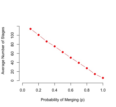
(a)

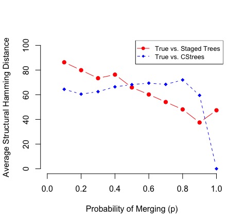
(b)

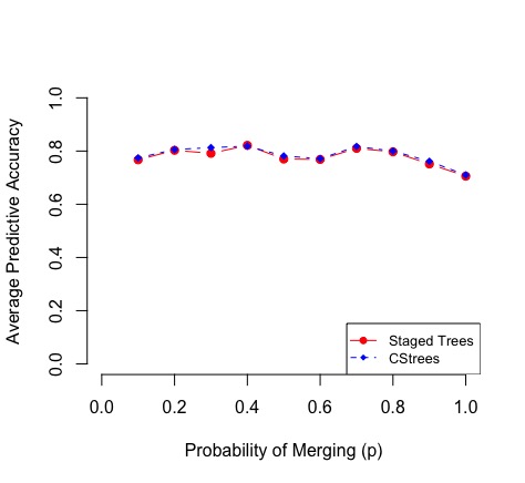
(c)

Figure 9. (a) Average number of stages of $10$ random binary staged trees on $7$ variables for each merging probability $p\in\{0.1,0.2,\ldots,0.9,1.0\}$ (b) Average structural Hamming distances to the true stage tree (c) Average predictive accuracies of the learned trees.

We implemented a naive algorithm, which we call BHC-CS, that learns from iid samples $\mathbb{D}$ a CStree on $n$ variables with a known causal ordering by considering, for $k\in\{2,\ldots,n-1\}$ all possible pairwise mergings of stages in level $L_{k-1}$ – where each merging is done to (minimally) ensure the resulting tree is also a CStree – and then picks the BIC-optimal merging. When there is no longer any merging that increases BIC, the algorithm moves to level $L_{k}$ and repeats the process. By Proposition 3.8, this is a consistent algorithm for learning CStrees with a known causal ordering. Our algorithm is the CStree equivalent of the backwards hill-climbing algorithm for learning staged trees (Carli et al., 2020), which we denote BHC-S.

To relate the performance of a learned CStree to a learned staged tree, we let the BHC-CS and BHC-S attempt to learn each true (i.e., data-generating) staged tree based on the training data. For each $p$, we report the average structural Hamming distance between the true staged tree and the learned trees in Figure 9(b). As expected, the trees learned by BHC-S are closer to the true trees than the learned CStrees, particularly for moderately sparse trees where the true tree can assume many more staging patterns than sparse CStrees. This is because, in most cases, the data-generating tree will not be a CStree, and hence the best we can hope for is a decent approximation of the true tree.

While the learned CStrees are only approximations of the true staged tree, we find that they function equally as well as the learned staged trees. To see this, we performed a posterior predictive check using the ten validation samples. For each value of $p$ and each variable $X_{i}$, the learned trees were tasked with predicting the value of $X_{i}$ in each validation sample given the values of all remaining variables. The average predictive accuracy (i.e., the average proportion of times each tree correctly predicted the missing value) is recorded in Figure 9(c). We see that, despite learned CStrees only being able to approximate the true staged tree, their average predictive accuracy is essentially the same as that of the learned staged trees. This suggests that one can safely use CStrees without sacrificing predictive accuracy while gaining the representation results for CStrees proven in the previous sections.

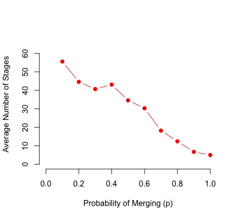
(a)

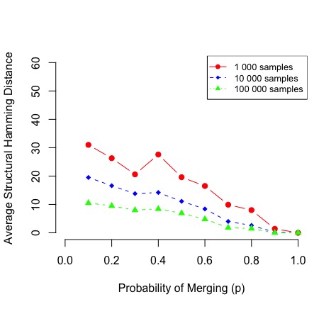
(b)

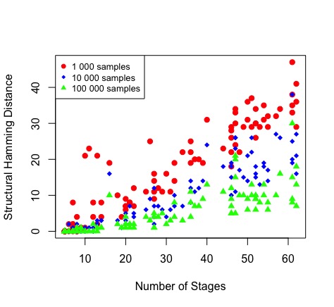
(c)

Figure 10. (a) the average number of stages for 10 randomly generated CStrees on $6$ binary variables for each merging probability $p$. (b) the average structural Hamming distances of the learned CStrees from the true CStree based on $1,000$, $10,000$ and $100,000$ samples. (c) the number of stages versus structural Hamming distance for each of the $100$ models.

According to Figure 9(b), despite being consistent, the backwards hill-climbing algorithms appear to rarely learn the true tree. This is attributable to the sample size required to exactly learn the stages in the higher levels of the trees. To see the consistency of BHC-CS in practice, we can increase the sample size and observe a decrease in structural Hamming distance as depicted in Figures 10(b) and 10(c) for sample sizes $1,000$, $10,000$ and $100,000$ drawn from random binary CStrees on $6$ binary variables. The random CStrees are constructed analogously to the random staged trees for the previous experiment. However, the merging of stages in each level so as to always produce a CStree can quickly lead to much sparser models. So the number of Bernoulli trials (for level $L_{k-1}$ and merging probability $p$) was adjusted to be $\lfloor 2^{k-1}/(1+4k(p-p^{2}))\rfloor$. This adjustment yields an approximately linear expected number of stages, as depicted in Figure 10(a). Figure 10(b) demonstrates that increasing the sample size strictly improves our estimates of the true CStree. Figure 10(c), which compares the number of stages of each of the true CStrees with its structural Hamming distance from the learned CStree, suggests that for at least $10,000$ samples, the learned CStree is quite close to the true CStree when the true tree has at most $1/3$ of the number of possible stages for a binary CStree on $6$ variables – 64. For the same sparsity level, we see that $100,000$ samples appears sufficient to learn almost all of the CStrees exactly.

6. Applications to Real Data

We apply the results on CStrees and interventional CStrees to two real data sets, demonstrating how the alternative representation of a (interventional) CStree via its context graphs allows us to quickly read context-specific causal information inferred from data. The first data set is purely observational and it studies risk factors in coronary heart disease; it is available with the R (R Core Team, 2020) package bnlearn (Scutari, 2010). The second data set is a mixture of observational and interventional data on the regulation of the expression of proteins critical to learning in mice; it is available at the UCI Machine Learning Repository (Dua and Graff, 2017). The code is available at (Duarte and Solus, 2021b).

6.1. Coronary heart disease data

The data set coronary, included in the bnlearn package, contains samples from $1814$ men measuring probable risk factors for coronary heart disease with binary variables. The list of variables with their outcome set is: $S\!\!:$ smoking $\{\text{``no'',``yes''}\}$, $MW\!\!:$ strenuous mental work $\{\text{``no'',``yes''}\}$, $PW\!\!:$ strenuous physical work, $\{\text{``no'',``yes''}\}$, $P\!\!:$ systolic blood pressure, $\{(>\!\!140),(<\!\!140)\}$, $L\!\!:$ ratio of $\beta$ to $\alpha$-lipoproteins $\{(<\!\!3),(>\!\!3)\}$, and $F\!\!:$ family history of coronary heart disease $\{\text{``negative'',``positive''}\}$. For the CStree depicted in Figure 11, an arrow pointing downwards indicates the first outcome of the variable at that level, and one pointing upwards indicates the second outcome.

To learn the BIC-optimal CStree given data on six binary variables, we would have to score $1.1362\times 10^{22}$ models, which is on the order of the number of DAGs (or MECs of DAGs) on $11$ variables. To limit the exponential blow-up in the number of computations needed, we employ the BHC-CS algorithm introduced in Section 5. Since BHC-CS assumes a known causal ordering of the tree, we run BHC-CS one time for each of the $6!=720$ causal orderings and then select the BIC-optimal output over all of these runs, an adaptation we refer to as BHC-CS-perm. Since the sample size is roughly $2,000$, assuming the underlying CStree structure is sparse, we can expect a decent approximation of the data-generating structure based on the simulations in Figure 10. The learned CStree is depicted in Figure 11(a).

(a) Learned CStree $\mathcal{T}_{\texttt{coronary}}$.

(b) Minimal context graphs $\mathcal{G}_{\mathcal{T}_{\texttt{coronary}}}$.

Figure 11. The CStree learned by BHC-CS-perm for the coronary data set.

The tree depicted in Figure 11(a) has a total of 15 stages, which is less than a third of the possible 64 stages for a binary CStree on $6$ variables. There are $7$ non-singleton stages which, respectively, have the following associated CSI relations via Lemma 3.1:

$$PW\mathchoice{\mathrel{\hbox to0.0pt{$\displaystyle\perp$\hss}\mkern 2.0mu{\displaystyle\perp}}}{\mathrel{\hbox to0.0pt{$\textstyle\perp$\hss}\mkern 2.0mu{\textstyle\perp}}}{\mathrel{\hbox to0.0pt{$\scriptstyle\perp$\hss}\mkern 2.0mu{\scriptstyle\perp}}}{\mathrel{\hbox to0.0pt{$\scriptscriptstyle\perp$\hss}\mkern 2.0mu{\scriptscriptstyle\perp}}}P\mid MW=\mbox{yes},\,\,S\mathchoice{\mathrel{\hbox to0.0pt{$\displaystyle\perp$\hss}\mkern 2.0mu{\displaystyle\perp}}}{\mathrel{\hbox to0.0pt{$\textstyle\perp$\hss}\mkern 2.0mu{\textstyle\perp}}}{\mathrel{\hbox to0.0pt{$\scriptstyle\perp$\hss}\mkern 2.0mu{\scriptstyle\perp}}}{\mathrel{\hbox to0.0pt{$\scriptscriptstyle\perp$\hss}\mkern 2.0mu{\scriptscriptstyle\perp}}}MW,PW\mid P=(>140),\,\,S\mathchoice{\mathrel{\hbox to0.0pt{$\displaystyle\perp$\hss}\mkern 2.0mu{\displaystyle\perp}}}{\mathrel{\hbox to0.0pt{$\textstyle\perp$\hss}\mkern 2.0mu{\textstyle\perp}}}{\mathrel{\hbox to0.0pt{$\scriptstyle\perp$\hss}\mkern 2.0mu{\scriptstyle\perp}}}{\mathrel{\hbox to0.0pt{$\scriptscriptstyle\perp$\hss}\mkern 2.0mu{\scriptscriptstyle\perp}}}MW\mid P=(<140),PW=\mbox{yes},$$

$$L\mathchoice{\mathrel{\hbox to0.0pt{$\displaystyle\perp$\hss}\mkern 2.0mu{\displaystyle\perp}}}{\mathrel{\hbox to0.0pt{$\textstyle\perp$\hss}\mkern 2.0mu{\textstyle\perp}}}{\mathrel{\hbox to0.0pt{$\scriptstyle\perp$\hss}\mkern 2.0mu{\scriptstyle\perp}}}{\mathrel{\hbox to0.0pt{$\scriptscriptstyle\perp$\hss}\mkern 2.0mu{\scriptscriptstyle\perp}}}MW,PW,P\mid S=\mbox{no},\quad L\mathchoice{\mathrel{\hbox to0.0pt{$\displaystyle\perp$\hss}\mkern 2.0mu{\displaystyle\perp}}}{\mathrel{\hbox to0.0pt{$\textstyle\perp$\hss}\mkern 2.0mu{\textstyle\perp}}}{\mathrel{\hbox to0.0pt{$\scriptstyle\perp$\hss}\mkern 2.0mu{\scriptstyle\perp}}}{\mathrel{\hbox to0.0pt{$\scriptscriptstyle\perp$\hss}\mkern 2.0mu{\scriptscriptstyle\perp}}}MW,PW\mid S=\mbox{yes},P=(>140),$$

$$L\mathchoice{\mathrel{\hbox to0.0pt{$\displaystyle\perp$\hss}\mkern 2.0mu{\displaystyle\perp}}}{\mathrel{\hbox to0.0pt{$\textstyle\perp$\hss}\mkern 2.0mu{\textstyle\perp}}}{\mathrel{\hbox to0.0pt{$\scriptstyle\perp$\hss}\mkern 2.0mu{\scriptstyle\perp}}}{\mathrel{\hbox to0.0pt{$\scriptscriptstyle\perp$\hss}\mkern 2.0mu{\scriptscriptstyle\perp}}}MW\mid S=\mbox{yes},PW=\mbox{yes},P=(<140),\quad\mbox{and}\quad F\mathchoice{\mathrel{\hbox to0.0pt{$\displaystyle\perp$\hss}\mkern 2.0mu{\displaystyle\perp}}}{\mathrel{\hbox to0.0pt{$\textstyle\perp$\hss}\mkern 2.0mu{\textstyle\perp}}}{\mathrel{\hbox to0.0pt{$\scriptstyle\perp$\hss}\mkern 2.0mu{\scriptstyle\perp}}}{\mathrel{\hbox to0.0pt{$\scriptscriptstyle\perp$\hss}\mkern 2.0mu{\scriptscriptstyle\perp}}}S,MW,PW,P,L.$$

The context for each of the above CSI relations is the stage-defining context for its associated stage. By taking the context-specific closure of these seven CSI relations, we recover the minimal context graphs $\mathcal{G}_{\mathcal{T}_{\texttt{coronary}}}$ depicted in Figure 11(b).

The empty context for $\mathcal{T}_{\texttt{coronary}}$ is the complete DAG on $MW,PW,P,S$ and $L$ with $F$ independent of all other variables. DAG learning algorithms such as those in the bnlearn package in R learn DAGs for this data set with similar structure: $F$ adjacent to only one variable and only two non-adjacencies among the remaining variables. However, the CStree structure reveals context-specific causal information that is overlooked by such DAG models. For instance, the context graph $\mathcal{G}_{MW=\mbox{yes}}$ encodes two v-structures, purporting physically strenous work ($PW$) and systolic blood pressure ($P$) as independent predictors of both smoking ($S$) and the ratio of $\beta$ to $\alpha$-lipoproteins ($L$) in the context that the individual has mentally strenuous work ($MW=\mbox{yes}$). By Corollary 3.6, any CStree statistically equivalent to $\mathcal{T}_{\texttt{coronary}}$ must have the same minimal contexts and same skeleta and v-structures in each of its minimal context graphs. Hence, the presence of these two v-structures also fixes the directions of these arrows in the empty context graph $\mathcal{G}_{\emptyset}$, thereby providing more refined causal information than carried by the lone DAG $\mathcal{G}_{\emptyset}$. The representation theorem (Theorem 3.3) and the resulting characterization of statistical equivalence (Corollary 3.6) allow us to easily see these causal relations directly from the context graphs, without any further analysis that may be required to deduce the same results by working only with the staged tree representation $\mathcal{T}_{\texttt{coronary}}$. In a similar fashion, one can quickly read off context-specific conditional independence relations from the context-graphs that may be difficult to deduce directly from the staged tree representation. For example, we see directly from the context graph $\mathcal{G}_{P=(>140)}$ that physically strenuous work and mentally strenuous work are independent from smoking and the ratio of $\beta$ to $\alpha$-lipoproteins in the context that systolic blood pressure is high ($P=(>140)$). In general, reading CSI relations $X_{A}\mathchoice{\mathrel{\hbox to0.0pt{$\displaystyle\perp$\hss}\mkern 2.0mu{\displaystyle\perp}}}{\mathrel{\hbox to0.0pt{$\textstyle\perp$\hss}\mkern 2.0mu{\textstyle\perp}}}{\mathrel{\hbox to0.0pt{$\scriptstyle\perp$\hss}\mkern 2.0mu{\scriptstyle\perp}}}{\mathrel{\hbox to0.0pt{$\scriptscriptstyle\perp$\hss}\mkern 2.0mu{\scriptscriptstyle\perp}}}X_{B}\mid X_{S},X_{C}=x_{C}$ where $A$ and $B$ are not singletons from a staged tree can be a challenging task, but it becomes straight-forward by restricting to CStrees and utilizing their representation via minimal context-graphs.

6.2. Mice protein expression data

The data set available at the UCI Machine Learning Repository (Dua and Graff, 2017) records expression levels of $77$ different proteins/protein modifications measured in the cerebral cortex of mice. Each mouse is either a control or a Ts65Dn trisomic Down Syndrome mouse. Each mouse was either injected with saline or treated with the drug memantine, which is believed to affect associative learning in mice. The mice were then trained in context fear conditioning (CFC), a task used to assess associative learning (Radulovic et al., 1998). The standard CFC protocol divides mice into two groups: the context-shock (CS) group, which is placed into a novel cage, allowed to explore, and then receives a brief electric shock, and the shock-context (SC) group, which is placed in the novel cage, immediately given the electric shock, and thereafter is allowed to explore. The expression levels of $77$ different proteins were measured from eight different classes of mice, defined by whether the mouse is control (c) or trisomic (t), received memantine (m) or saline (s), and whether it was in a CS or SC group for the learning task. The eight classes are denoted as c-CS-s, c-CS-m, c-SC-s, c-SC-m, t-CS-s, t-CS-m, t-SC-s, t-SC-m. There are $9,10,9,10,7,9,9$, and $9$ mice in each class, respectively. Fifteen measurements of each protein were registered per mouse, yielding a total of $1080$ measurements per protein. Each measurement is regarded as an independent sample.

In the following, we treat the $135$ measurements taken from the group c-SC-s as observational data and the $150$ measurements taken from the group c-SC-m as interventional data, taking treatment with memantine as our intervention. We consider the expression levels of four proteins, each of which is believed to discriminate between between the classes c-SC-s and c-SC-m (see (Higuera et al., 2015, Table 3, Column 2)). As our models are for discrete random variables only, we discretized the data set using the quantile method. The result is four binary random variables, one for each protein considered, with outcomes “high (expression level)” and “low (expression level).” Hence, our goal is to learn an optimal interventional CStree on four binary variables given the observational data and one interventional data set. Here, we assume that the intervention targets are unknown since we cannot be certain which proteins, at which expression levels (i.e. in which contexts), are directly targeted by the drug memantine.

There are $59,136$ CStrees on four binary random variables. As the intervention targets are latent, we need to consider all possible interventions in a given observational CStree. For a CStree on four binary variables, the number of models to be scored can be as large as $2^{15}$. To avoid the time complexity issues of testing many models for each of $59136$ trees, we instead first learn the BIC-optimal equivalence class of CStrees for the data and then score all possible interventional CStrees that arise by targeting any subset of the stages in any element of this equivalence class.

6.2.1. pCAMKII, pPKCG, NR1 and pS6

A representative of the BIC-optimal equivalence class for the observational data with the proteins pCAMKII, pPKCG, NR1 and pS6 is given in Figure 12; its context graphs are depicted in Figure 13.

Figure 12. An element of the BIC-optimal equivalence class of CStrees for the observational data for the proteins pCAMKII, pPKCG, NR1 and pS6.

Figure 13. The context graphs for the CStree depicted in Figure 12.

According to Corollary 3.6, the CStree in Figure 12 is in an equivalence class of size two, where the other element is given by swapping pCAMKII and pS6 in the causal ordering. This corresponds to reversing the arrow between these two nodes in the graph $\mathcal{G}_{pPKCG=low}$. Notice also that the arrow pPKCG$\to$NR1 is covered in the DAG $\mathcal{G}_{\emptyset}$, and hence reversing this arrow would result in a Markov equivalent DAG. However, according to Corollary 3.6, this arrow is fixed among all elements of the equivalence class due to the v-structure in the context graph $\mathcal{G}_{pCAMKII=high}$.

Figure 14. The BIC-optimal interventional CStree on the variables pCAMKII, pPKCG, NR1 and pS6.

We can try to use our interventional data drawn from the class c-SC-m to distinguish between the two elements of this equivalence class, and hence determine the complete causal ordering of the variables. We compute the BIC-optimal interventional CStree that arises from any choice of nonempty complete interventions targets in either of the two elements of the observational equivalence class. The resulting BIC-optimal interventional CStree is depicted in Figure 14, and its interventional contexts graphs are given in Figure 15.

Figure 15. The context graphs for the interventional CStree depicted in Figure 14.

Comparing these two figures, we already see how the representation of an interventional CStree via its context graphs is more compact and easier to read than its staged tree representation. We also see that precisely one stage is targeted for intervention and it is in the context pCAMKII = high. Hence, the interventional context graphs contain two arrows pointing from an interventional node $w_{mem}$ (representing intervention via memantine) into the node pPKCG, one arrow in the $\mathcal{G}_{\emptyset}$ and the other in $\mathcal{G}_{pCAMKII=high}$. Note that no arrow is added to $\mathcal{G}_{pCAMKII=low}$, as no stages in this context were targeted by the intervention. While this intervention introduces new v-structures, none of the new v-structures fix edges that were not already fixed in the observational context graphs. Hence, a targeted intervention at pCAMKII or pS6 in the context that pPKCG = low is needed to distinguish the true causal structure among the proteins.

6.2.2. pPKCG, pNUMB, pNR1 and pCAMKII

To illustrate the refinement of equivalence classes via intervention, we can consider another set of four proteins: pPKCG, pNUMB, pNR1 and pCAMKII. A representative of the BIC-optimal equivalence class given the observational data for these four proteins is depicted in Figure 16, and its representation as a sequence of context graphs is in Figure 17. Via Corollary 3.6, one can deduce that the equivalence class of the CStree in Figure 16 contains three additional CStrees, which are shown in Figure 20 in Appendix B.

Figure 16. An element of the BIC optimal equivalence class of CStrees for the observational mice data.

Figure 17. The context graphs for the CStree depicted in Figure 16.

We compute the BIC of every interventional CStree that arises for a set of valid intervention targets in one of the CStrees in the equivalence class of the tree in Figure 16. Given the (finite) data, the highest BIC score is achieved four times by the trees making up two different equivalence classes of interventional CStrees, each having only complete intervention targets. The interventional context graphs of these two classes are depicted in Figure 18, and the four trees appear in Figures 21 and 22 in Appendix B. By Theorem 4.2, we see directly from Figure 18(a) that the BIC-optimal interventional CStree with these contexts graphs is in an equivalence class of size one, whereas there are three trees in the equivalence class represented by Figure 18(b). As the BIC score cannot distinguish between these two equivalence classes given the small sample size we performed a bootstrap, producing $1000$ replicates and computing the BIC score for both equivalence classes for each replicate. The mean of the bootstrapped BICs is slightly higher for the equivalence class of size one. Hence, we take the context graphs in Figure 18(a) to be the context-specific causal structure of the data-generating interventional setting.

(a)  

(b)  

Figure 18. The context graphs representing the two different equivalence classes of the four BIC-optimal interventional CStrees.

7. Discussion

Among the features of DAG models that make them so successful in practice is their admittance of a global Markov property, which provides a combinatorial criterion describing the conditional independence relations satisfied by any distribution that factorizes according to the given DAG. The global Markov property for DAGs leads to the many combinatorial characterizations of model equivalence (Andersson and Perlman, 1997; Chickering, 1995; Verma and Pearl, 1990b) that drive some of the most popular causal discovery algorithms to date (Chickering, 2002; Solus et al., 2021; Spirtes et al., 2000).

From this perspective, the results established in this paper purport CStrees as the natural extension of DAG models to a family capable of expressing diverse context-specific conditional independence relations while maintaining the intuitive representation of a DAG. CStrees admit a global Markov property generalizing that of DAGs (Theorem 3.3), which leads to a characterization of model equivalence that generalizes a classical characterization of DAG model equivalence (Corollary 3.6). Moreover, these results generalize to interventional models (Section 4), making CStrees the first family of context-specific interventional models admitting a characterization of model equivalence. As we saw in real data examples (e.g., Figure 11), the representation of a CStree via its sequence of contexts graphs offers the user a quick way to read context-specific causal information, whereas reading the same information from the staged tree or CEG representation requires a more careful analysis. The simulations in Section 5 further suggest that one can safely model with a CStree instead of a more general staged tree without sacrificing predictive accuracy. Moreover, the BIC is a locally consistent scoring criterion for CStrees (Proposition 3.8), setting the stage for the development of consistent CStree learning algorithms that are more efficient than the naive BHC-CS-perm algorithm implemented in Subsection 6.1.

Natural directions for future research include a context-specific PC algorithm for learning CStrees and a similar extension of the Greedy Equivalence Search (GES) (Chickering, 2002). The observation that BIC is locally consistent for CStrees suggests that Meek’s Conjecture (Chickering, 2002, Theorem 4) could be extended to this family of models. The development of a consistent extension of GES to CStrees would provide a faster alternative to BHC-CS-perm, which necessarily considers all possible causal orderings of the tree (similar to the greedy permutation search (GSP) (Raskutti and Uhler, 2018) for DAGs). The results of Section 4 also suggest that the recent causal discovery algorithms that incorporate a mixture of observational and interventional data (Hauser and Bühlmann, 2012; Kocaoglu et al., 2019; Wang et al., 2017; Yang et al., 2018) can likely be extended to the context-specific setting via CStrees. Finally, it would also be interesting to see extensions of CStree models to the non-discrete data and/or causally insufficient settings.

Appendix A Proofs Omitted From the Main Text

A.1. Proof of Lemma 3.1

To prove the statement, we need to show that

$$f(x_{k}\mid\mathbf{x}_{[k-1]\setminus C_{i}},\mathbf{x}_{C_{i}})=f(x_{k}\mid\mathbf{x}_{C_{i}})$$

for any $f(x_{k},\mathbf{x}_{[k-1]\setminus C_{i}},\mathbf{x}_{C_{i}})>0$, where $C_{i}=\bigcap_{v\in S_{i}}v$ and $\mathbf{x}_{C_{i}}:=\mathbf{y}_{C_{i}}$ for any $\mathbf{y}\in S_{i}$. Since $\mathcal{T}\in\mathcal{T}_{\mathop{\rm CS}\nolimits}$ then it is uniform, stratified and compatibly-labeled. Hence, it follows for any $v,w\in S_{i}$ with $v=\mathbf{x}:=x_{1}\cdots x_{k-1}$ and $w=\mathbf{x}^{\prime}:=x_{1}^{\prime}\cdots x_{k-1}^{\prime}$

$$f(X_{k}\mid x_{1}\cdots x_{k-1})=f(X_{k}\mid x_{1}^{\prime}\cdots x_{k-1}^{\prime}).$$

Furthermore, since $\mathcal{T}\in\mathcal{T}_{\mathop{\rm CS}\nolimits}$, then there exists some $C\subset[k]$ and $\mathbf{x}_{C}\in\mathcal{R}_{C}$ such that $S_{i}$ is exactly the collection of vertices $\mathbf{y}$ in $L_{k}$ satisfying $\mathbf{y}_{C}=\mathbf{x}_{C}$. Hence, $C=C_{i}$. It follows that

$$f(X_{k}\mid X_{C_{i}}=\mathbf{x}_{C_{i}},\mathbf{x}_{[k-1]\setminus C_{i}})=f(X_{k}\mid X_{C_{i}}=\mathbf{x}_{C_{i}},\mathbf{x}_{[k-1]\setminus C_{i}}^{\prime}).$$

Since $\mathcal{T}\in\mathcal{T}_{\mathop{\rm CS}\nolimits}$, it follows that this equality holds for any $\mathbf{x}_{[k-1]\setminus C_{i}}^{\prime}\in\mathcal{R}_{[k-1]\setminus C_{i}}$. This fact is equivalent to $X_{k}\mathchoice{\mathrel{\hbox to0.0pt{$\displaystyle\perp$\hss}\mkern 2.0mu{\displaystyle\perp}}}{\mathrel{\hbox to0.0pt{$\textstyle\perp$\hss}\mkern 2.0mu{\textstyle\perp}}}{\mathrel{\hbox to0.0pt{$\scriptstyle\perp$\hss}\mkern 2.0mu{\scriptstyle\perp}}}{\mathrel{\hbox to0.0pt{$\scriptscriptstyle\perp$\hss}\mkern 2.0mu{\scriptscriptstyle\perp}}}X_{[k-1]\setminus C_{i}}\mid X_{C_{i}}=\mathbf{x}_{C_{i}}$.

A.2. Proof of Lemma 3.2

Suppose that $X_{C}=\mathbf{x}_{C}\notin\mathcal{C}_{\mathcal{T}}$. Then, by definition of a minimal context, there must exist $\emptyset\neq T\subseteq C$ such that

$$X_{A}\mathchoice{\mathrel{\hbox to0.0pt{$\displaystyle\perp$\hss}\mkern 2.0mu{\displaystyle\perp}}}{\mathrel{\hbox to0.0pt{$\textstyle\perp$\hss}\mkern 2.0mu{\textstyle\perp}}}{\mathrel{\hbox to0.0pt{$\scriptstyle\perp$\hss}\mkern 2.0mu{\scriptstyle\perp}}}{\mathrel{\hbox to0.0pt{$\scriptscriptstyle\perp$\hss}\mkern 2.0mu{\scriptscriptstyle\perp}}}X_{B}\mid X_{S\cup T},X_{C\setminus T}=\mathbf{x}_{C\setminus T}\in\mathcal{J}(\mathcal{T}).$$

Picking $T$ to be any maximal subset of $C$ with respect to this property yields $X_{C\setminus T}=\mathbf{x}_{C\setminus T}\in\mathcal{C}_{\mathcal{T}}$, and hence $X_{C}=\mathbf{x}_{C}$ has the minimal context $X_{C\setminus T}=\mathbf{x}_{C\setminus T}$ as a subcontext.

By Lemma 3.1, for any stage $S_{i}\subset L_{k-1}$

$$X_{k}\mathchoice{\mathrel{\hbox to0.0pt{$\displaystyle\perp$\hss}\mkern 2.0mu{\displaystyle\perp}}}{\mathrel{\hbox to0.0pt{$\textstyle\perp$\hss}\mkern 2.0mu{\textstyle\perp}}}{\mathrel{\hbox to0.0pt{$\scriptstyle\perp$\hss}\mkern 2.0mu{\scriptstyle\perp}}}{\mathrel{\hbox to0.0pt{$\scriptscriptstyle\perp$\hss}\mkern 2.0mu{\scriptscriptstyle\perp}}}X_{[k-1]\setminus C_{i}}\mid X_{C_{i}}=\mathbf{x}_{C_{i}}\in\mathcal{J}(\mathcal{T}),$$

and by definition those statements generate $\mathcal{J}(\mathcal{T})$. Notice that the only two context-specific conditional independence axioms that change the context $X_{C}=\mathbf{x}_{C}$ are specialization and absorption. Since specialization can never produce a minimal context, then they can only be produced by an application of the absorption axiom. However, any statement $X_{A}\mathchoice{\mathrel{\hbox to0.0pt{$\displaystyle\perp$\hss}\mkern 2.0mu{\displaystyle\perp}}}{\mathrel{\hbox to0.0pt{$\textstyle\perp$\hss}\mkern 2.0mu{\textstyle\perp}}}{\mathrel{\hbox to0.0pt{$\scriptstyle\perp$\hss}\mkern 2.0mu{\scriptstyle\perp}}}{\mathrel{\hbox to0.0pt{$\scriptscriptstyle\perp$\hss}\mkern 2.0mu{\scriptscriptstyle\perp}}}X_{B}\mid X_{S\cup T},X_{C\setminus T}=\mathbf{x}_{C\setminus T}$ produced by applying absorption to a statement $X_{A}\mathchoice{\mathrel{\hbox to0.0pt{$\displaystyle\perp$\hss}\mkern 2.0mu{\displaystyle\perp}}}{\mathrel{\hbox to0.0pt{$\textstyle\perp$\hss}\mkern 2.0mu{\textstyle\perp}}}{\mathrel{\hbox to0.0pt{$\scriptstyle\perp$\hss}\mkern 2.0mu{\scriptstyle\perp}}}{\mathrel{\hbox to0.0pt{$\scriptscriptstyle\perp$\hss}\mkern 2.0mu{\scriptscriptstyle\perp}}}X_{B}\mid X_{S},X_{C}=\mathbf{x}_{C}$ will have context $X_{C\setminus T}=\mathbf{x}_{C\setminus T}$ as a subcontext of $X_{C}=\mathbf{x}_{C}$. Hence, each minimal context in $\mathcal{C}_{\mathcal{T}}$ must be a subcontext of (at least) one $X_{C_{i}}=\mathbf{x}_{C_{i}}$, the contexts of the generators of $\mathcal{J}(\mathcal{T})$.

A.3. Proof of Theorem 3.3

We first show that (1) and (2) are equivalent. Suppose that $f\in\mathcal{M}_{(\mathcal{T},\theta)}$. Then $f$ entails all context-specific conditional independence relations

$$X_{k}\mathchoice{\mathrel{\hbox to0.0pt{$\displaystyle\perp$\hss}\mkern 2.0mu{\displaystyle\perp}}}{\mathrel{\hbox to0.0pt{$\textstyle\perp$\hss}\mkern 2.0mu{\textstyle\perp}}}{\mathrel{\hbox to0.0pt{$\scriptstyle\perp$\hss}\mkern 2.0mu{\scriptstyle\perp}}}{\mathrel{\hbox to0.0pt{$\scriptscriptstyle\perp$\hss}\mkern 2.0mu{\scriptscriptstyle\perp}}}X_{[k-1]\setminus C_{i}}\mid X_{C_{i}}=\mathbf{x}_{C_{i}}$$

from Lemma 3.1. Hence, $f$ is Markov to $\mathcal{J}(\mathcal{T})$, and therefore entails all context-specific conditional independence relations in $\mathcal{J}_{X_{C}=\mathbf{x}_{C}}$, for each $X_{C}=\mathbf{x}_{C}\in\mathcal{C}_{\mathcal{T}}$.

Conversely, suppose that $f\in\mathcal{M}(\mathcal{G}_{\mathcal{T}})$. Then for all $X_{C}=\mathbf{x}_{C}\in\mathcal{C}_{\mathcal{T}}$, $f$ entails $X_{A}\mathchoice{\mathrel{\hbox to0.0pt{$\displaystyle\perp$\hss}\mkern 2.0mu{\displaystyle\perp}}}{\mathrel{\hbox to0.0pt{$\textstyle\perp$\hss}\mkern 2.0mu{\textstyle\perp}}}{\mathrel{\hbox to0.0pt{$\scriptstyle\perp$\hss}\mkern 2.0mu{\scriptstyle\perp}}}{\mathrel{\hbox to0.0pt{$\scriptscriptstyle\perp$\hss}\mkern 2.0mu{\scriptscriptstyle\perp}}}X_{B}\mid X_{S},X_{C}=\mathbf{x}_{C}$ whenever $A$ and $B$ are d-separated given $S$ in the minimal I-MAP $\mathcal{G}_{X_{C}=\mathbf{x}_{C}}$ of $\mathcal{J}_{X_{C}=\mathbf{x}_{C}}$. To see that $f$ factorizes according to $\mathcal{T}$, it suffices to show that, for all $k\in[p-1]$, and all stages $S_{i}$ in level $L_{k-1}$, $f$ entails

$$X_{k}\mathchoice{\mathrel{\hbox to0.0pt{$\displaystyle\perp$\hss}\mkern 2.0mu{\displaystyle\perp}}}{\mathrel{\hbox to0.0pt{$\textstyle\perp$\hss}\mkern 2.0mu{\textstyle\perp}}}{\mathrel{\hbox to0.0pt{$\scriptstyle\perp$\hss}\mkern 2.0mu{\scriptstyle\perp}}}{\mathrel{\hbox to0.0pt{$\scriptscriptstyle\perp$\hss}\mkern 2.0mu{\scriptscriptstyle\perp}}}X_{[k-1]\setminus C_{i}}\mid X_{C_{i}}=\mathbf{x}_{C_{i}},$$ (4)

where $X_{C_{i}}=\mathbf{x}_{C_{i}}$ is the context associated to the stage $S_{i}$ in Lemma 3.1. By definition of $\mathcal{J}(\mathcal{T})$, each CSI relation (4) is in $\mathcal{J}(\mathcal{T})$. So by Lemma 3.2, either $X_{C_{i}}=\mathbf{x}_{C_{i}}\in\mathcal{C}_{\mathcal{T}}$ or there exists $C\subset C_{i}$ such that $X_{C}=\mathbf{x}_{C}=\mathbf{x}_{C_{i}\cap C}\in\mathcal{C}_{\mathcal{T}}$ and (4) is implied by the specialization of

$$X_{k}\mathchoice{\mathrel{\hbox to0.0pt{$\displaystyle\perp$\hss}\mkern 2.0mu{\displaystyle\perp}}}{\mathrel{\hbox to0.0pt{$\textstyle\perp$\hss}\mkern 2.0mu{\textstyle\perp}}}{\mathrel{\hbox to0.0pt{$\scriptstyle\perp$\hss}\mkern 2.0mu{\scriptstyle\perp}}}{\mathrel{\hbox to0.0pt{$\scriptscriptstyle\perp$\hss}\mkern 2.0mu{\scriptscriptstyle\perp}}}X_{[k-1]\setminus C_{i}}\mid X_{C_{i}\setminus C},X_{C}=\mathbf{x}_{C}\in\mathcal{J}_{X_{C}=\mathbf{x}_{C}}.$$ (5)

By weak union, it follows that

$$X_{k}\mathchoice{\mathrel{\hbox to0.0pt{$\displaystyle\perp$\hss}\mkern 2.0mu{\displaystyle\perp}}}{\mathrel{\hbox to0.0pt{$\textstyle\perp$\hss}\mkern 2.0mu{\textstyle\perp}}}{\mathrel{\hbox to0.0pt{$\scriptstyle\perp$\hss}\mkern 2.0mu{\scriptstyle\perp}}}{\mathrel{\hbox to0.0pt{$\scriptscriptstyle\perp$\hss}\mkern 2.0mu{\scriptscriptstyle\perp}}}X_{j}\mid X_{[k-1]\setminus(C_{i}\cup\{j\})},X_{C_{i}\setminus C},X_{C}=\mathbf{x}_{C}\in\mathcal{J}_{X_{C}=\mathbf{x}_{C}}$$

for all $j\in[k-1]\setminus C_{i}$, and hence, the minimal I-MAP $\mathcal{G}_{X_{C}=\mathbf{x}_{C}}$ does not contain the edges $j\rightarrow k$ for all $j\in[k-1]\setminus C_{i}$. Since independence models for DAGs are compositional (see (Sadeghi and Lauritzen, 2014)), it follows that $k$ and $[k-1]\setminus C_{i}$ are d-separated given $C_{i}\setminus C$ in $\mathcal{G}_{X_{C}=\mathbf{x}_{C}}$. Hence, $f$ entails the statements in (5). Applying specialization, it follows that $f$ entails the CSI relations in (4), and therefore factorizes according to $\mathcal{T}$.

We now show that (2) and (3) are equivalent. Let $X_{C}=\mathbf{x}_{C}\in\mathcal{C}_{\mathcal{T}}$, and set $g(X_{[p]\setminus C}):=f(X_{[p]\setminus C}\mid X_{C}=\mathbf{x}_{C})$. Since $f$ is Markov to $\mathcal{G}_{\mathcal{T}}$, whenever $A$ and $B$ are $d$-separated in $\mathcal{G}_{X_{C}=\mathbf{x}_{C}}$ given $S$, we have that $f$ entails $X_{A}\mathchoice{\mathrel{\hbox to0.0pt{$\displaystyle\perp$\hss}\mkern 2.0mu{\displaystyle\perp}}}{\mathrel{\hbox to0.0pt{$\textstyle\perp$\hss}\mkern 2.0mu{\textstyle\perp}}}{\mathrel{\hbox to0.0pt{$\scriptstyle\perp$\hss}\mkern 2.0mu{\scriptstyle\perp}}}{\mathrel{\hbox to0.0pt{$\scriptscriptstyle\perp$\hss}\mkern 2.0mu{\scriptscriptstyle\perp}}}X_{B}\mid X_{S},X_{C}=\mathbf{x}_{C}$; or equivalently,

$$\frac{f(\mathbf{x}_{A},\mathbf{x}_{B},\mathbf{x}_{S},\mathbf{x}_{C})}{f(\mathbf{x}_{B},\mathbf{x}_{S},\mathbf{x}_{C})}=\frac{f(\mathbf{x}_{A},\mathbf{x}_{S},\mathbf{x}_{C})}{f(\mathbf{x}_{S},\mathbf{x}_{C})},$$

for any $(\mathbf{x}_{A},\mathbf{x}_{B},\mathbf{x}_{S})\in\mathcal{R}_{A\cup B\cup S}$. Since for any $\mathbf{x}_{[p]\setminus C}\in\mathcal{R}_{[p]\setminus C}$,

$$g(\mathbf{x}_{[p]\setminus C})=\frac{1}{f(\mathbf{x}_{C})}f(\mathbf{x}_{[p]\setminus C},\mathbf{x}_{C}),$$

then

$$g(\mathbf{x}_{A},\mathbf{x}_{B},\mathbf{x}_{S})=\sum_{\mathbf{y}\in\mathcal{R}_{[p]\setminus A\cup B\cup C\cup S}}\frac{f(\mathbf{y},\mathbf{x}_{A},\mathbf{x}_{B},\mathbf{x}_{S},\mathbf{x}_{C})}{f(\mathbf{x}_{C})}=\frac{1}{f(\mathbf{x}_{C})}f(\mathbf{x}_{A},\mathbf{x}_{B},\mathbf{x}_{S},\mathbf{x}_{C}),$$

and similarly for $g(\mathbf{x}_{B},\mathbf{x}_{S}),g(\mathbf{x}_{A},\mathbf{x}_{S})$, and $g(\mathbf{x}_{S})$. Hence, whenever $A$ and $B$ are $d$-separated in $\mathcal{G}_{X_{C}=\mathbf{x}_{C}}$ given $S$, we have that

$$\frac{g(\mathbf{x}_{A},\mathbf{x}_{B},\mathbf{x}_{S})}{g(\mathbf{x}_{B},\mathbf{x}_{S})}=\frac{g(\mathbf{x}_{A},\mathbf{x}_{S})}{g(\mathbf{x}_{S})}.$$

Therefore, $g$ entails $X_{A}\mathchoice{\mathrel{\hbox to0.0pt{$\displaystyle\perp$\hss}\mkern 2.0mu{\displaystyle\perp}}}{\mathrel{\hbox to0.0pt{$\textstyle\perp$\hss}\mkern 2.0mu{\textstyle\perp}}}{\mathrel{\hbox to0.0pt{$\scriptstyle\perp$\hss}\mkern 2.0mu{\scriptstyle\perp}}}{\mathrel{\hbox to0.0pt{$\scriptscriptstyle\perp$\hss}\mkern 2.0mu{\scriptscriptstyle\perp}}}X_{B}\mid X_{S}$ whenever $A$ and $B$ are $d$-separated given $S$ in $\mathcal{G}_{X_{C}=\mathbf{x}_{C}}$ for all $X_{C}=\mathbf{x}_{C}\in\mathcal{C}_{\mathcal{T}}$ if and only if $f$ is Markov to $\mathcal{G}_{\mathcal{T}}$. It follows that $f$ is Markov to $\mathcal{G}_{\mathcal{T}}$ if and only if for all $X_{C}=\mathbf{x}_{C}\in\mathcal{C}_{\mathcal{T}}$,

$$\begin{split}f(X_{[p]\setminus C}\mid X_{C}=\mathbf{x}_{C})=g(X_{[p]\setminus C})&=\prod_{k\in[p]\setminus C}g(X_{k}\mid X_{\mathop{\rm pa}\nolimits_{\mathcal{G}_{X_{C}=\mathbf{x}_{C}}}(k)}),\\ &=\prod_{k\in[p]\setminus C}\frac{g(X_{k},X_{\mathop{\rm pa}\nolimits_{\mathcal{G}_{X_{C}=\mathbf{x}_{C}}}(k)})}{g(X_{\mathop{\rm pa}\nolimits_{\mathcal{G}_{X_{C}=\mathbf{x}_{C}}}(k)})},\\ &=\prod_{k\in[p]\setminus C}\frac{f(X_{k},X_{\mathop{\rm pa}\nolimits_{\mathcal{G}_{X_{C}=\mathbf{x}_{C}}}(k)},X_{C}=\mathbf{x}_{C})}{f(X_{\mathop{\rm pa}\nolimits_{\mathcal{G}_{X_{C}=\mathbf{x}_{C}}}(k)},X_{C}=\mathbf{x}_{C})},\\ &=\prod_{k\in[p]\setminus C}f(X_{k}\mid X_{\mathop{\rm pa}\nolimits_{\mathcal{G}_{X_{C}=\mathbf{x}_{C}}}(k)},X_{C}=\mathbf{x}_{C}),\\ \end{split}$$

which completes the proof.

A.4. Proof of Lemma 3.4

Suppose, for the sake of contradiction, that there exists $X_{C}=\mathbf{x}_{C}\in\mathcal{C}_{\mathcal{T}}$ such that $X_{C}=\mathbf{x}_{C}\notin\mathcal{C}_{\mathcal{T}^{\prime}}$. Then, by definition of the set $\mathcal{C}_{\mathcal{T}}$ and Lemma 3.2, there must exist a CSI relation $X_{A}\mathchoice{\mathrel{\hbox to0.0pt{$\displaystyle\perp$\hss}\mkern 2.0mu{\displaystyle\perp}}}{\mathrel{\hbox to0.0pt{$\textstyle\perp$\hss}\mkern 2.0mu{\textstyle\perp}}}{\mathrel{\hbox to0.0pt{$\scriptstyle\perp$\hss}\mkern 2.0mu{\scriptstyle\perp}}}{\mathrel{\hbox to0.0pt{$\scriptscriptstyle\perp$\hss}\mkern 2.0mu{\scriptscriptstyle\perp}}}X_{B}\mid X_{S},X_{C}=\mathbf{x}_{C}$ in $\mathcal{J}(\mathcal{T})$ that is not implied by specialization of any statement $X_{A}\mathchoice{\mathrel{\hbox to0.0pt{$\displaystyle\perp$\hss}\mkern 2.0mu{\displaystyle\perp}}}{\mathrel{\hbox to0.0pt{$\textstyle\perp$\hss}\mkern 2.0mu{\textstyle\perp}}}{\mathrel{\hbox to0.0pt{$\scriptstyle\perp$\hss}\mkern 2.0mu{\scriptstyle\perp}}}{\mathrel{\hbox to0.0pt{$\scriptscriptstyle\perp$\hss}\mkern 2.0mu{\scriptscriptstyle\perp}}}X_{B}\mid X_{S\cup T},X_{C\setminus T}=\mathbf{x}_{C\setminus T}$. Since $X_{C}=\mathbf{x}_{C}\notin\mathcal{C}_{\mathcal{T}^{\prime}}$, it follows that either $X_{A}\mathchoice{\mathrel{\hbox to0.0pt{$\displaystyle\perp$\hss}\mkern 2.0mu{\displaystyle\perp}}}{\mathrel{\hbox to0.0pt{$\textstyle\perp$\hss}\mkern 2.0mu{\textstyle\perp}}}{\mathrel{\hbox to0.0pt{$\scriptstyle\perp$\hss}\mkern 2.0mu{\scriptstyle\perp}}}{\mathrel{\hbox to0.0pt{$\scriptscriptstyle\perp$\hss}\mkern 2.0mu{\scriptscriptstyle\perp}}}X_{B}\mid X_{S},X_{C}=\mathbf{x}_{C}$ is not a CSI relation in $\mathcal{J}(\mathcal{T}^{\prime})$ or there exists some subcontext $X_{C\setminus T}=\mathbf{x}_{C\setminus T}\in\mathcal{C}_{\mathcal{T}^{\prime}}$ such that the statement $X_{A}\mathchoice{\mathrel{\hbox to0.0pt{$\displaystyle\perp$\hss}\mkern 2.0mu{\displaystyle\perp}}}{\mathrel{\hbox to0.0pt{$\textstyle\perp$\hss}\mkern 2.0mu{\textstyle\perp}}}{\mathrel{\hbox to0.0pt{$\scriptstyle\perp$\hss}\mkern 2.0mu{\scriptstyle\perp}}}{\mathrel{\hbox to0.0pt{$\scriptscriptstyle\perp$\hss}\mkern 2.0mu{\scriptscriptstyle\perp}}}X_{B}\mid X_{S},X_{C}=\mathbf{x}_{C}$ is implied by the statement $X_{A}\mathchoice{\mathrel{\hbox to0.0pt{$\displaystyle\perp$\hss}\mkern 2.0mu{\displaystyle\perp}}}{\mathrel{\hbox to0.0pt{$\textstyle\perp$\hss}\mkern 2.0mu{\textstyle\perp}}}{\mathrel{\hbox to0.0pt{$\scriptstyle\perp$\hss}\mkern 2.0mu{\scriptstyle\perp}}}{\mathrel{\hbox to0.0pt{$\scriptscriptstyle\perp$\hss}\mkern 2.0mu{\scriptscriptstyle\perp}}}X_{B}\mid X_{S\cup T},X_{C\setminus T}=\mathbf{x}_{C\setminus T}$ encoded by $\mathcal{G}_{X_{C\setminus T}=\mathbf{x}_{C\setminus T}}^{\prime}\in\mathcal{G}_{\mathcal{T}^{\prime}}$. It follows from Theorem 3.3 that the statement $X_{A}\mathchoice{\mathrel{\hbox to0.0pt{$\displaystyle\perp$\hss}\mkern 2.0mu{\displaystyle\perp}}}{\mathrel{\hbox to0.0pt{$\textstyle\perp$\hss}\mkern 2.0mu{\textstyle\perp}}}{\mathrel{\hbox to0.0pt{$\scriptstyle\perp$\hss}\mkern 2.0mu{\scriptstyle\perp}}}{\mathrel{\hbox to0.0pt{$\scriptscriptstyle\perp$\hss}\mkern 2.0mu{\scriptscriptstyle\perp}}}X_{B}\mid X_{S\cup T},X_{C\setminus T}=\mathbf{x}_{C\setminus T}$ is in $\mathcal{J}(\mathcal{T}^{\prime})$. However, such a statement cannot be in $\mathcal{J}(\mathcal{T})$, as this would imply that the statement $X_{A}\mathchoice{\mathrel{\hbox to0.0pt{$\displaystyle\perp$\hss}\mkern 2.0mu{\displaystyle\perp}}}{\mathrel{\hbox to0.0pt{$\textstyle\perp$\hss}\mkern 2.0mu{\textstyle\perp}}}{\mathrel{\hbox to0.0pt{$\scriptstyle\perp$\hss}\mkern 2.0mu{\scriptstyle\perp}}}{\mathrel{\hbox to0.0pt{$\scriptscriptstyle\perp$\hss}\mkern 2.0mu{\scriptscriptstyle\perp}}}X_{B}\mid X_{S},X_{C}=\mathbf{x}_{C}$ is obtained by specialization from a statement of the form $X_{A}\mathchoice{\mathrel{\hbox to0.0pt{$\displaystyle\perp$\hss}\mkern 2.0mu{\displaystyle\perp}}}{\mathrel{\hbox to0.0pt{$\textstyle\perp$\hss}\mkern 2.0mu{\textstyle\perp}}}{\mathrel{\hbox to0.0pt{$\scriptstyle\perp$\hss}\mkern 2.0mu{\scriptstyle\perp}}}{\mathrel{\hbox to0.0pt{$\scriptscriptstyle\perp$\hss}\mkern 2.0mu{\scriptscriptstyle\perp}}}X_{B}\mid X_{S\cup T},X_{C\setminus T}=\mathbf{x}_{C\setminus T}$ in $\mathcal{J}(\mathcal{T})$. This latter fact would contradict our initial assumption that $X_{C}=\mathbf{x}_{C}$ is a minimal context. Hence, we may assume that there is a minimal context $X_{C}=\mathbf{x}_{C}$, such that the CSI relation $X_{A}\mathchoice{\mathrel{\hbox to0.0pt{$\displaystyle\perp$\hss}\mkern 2.0mu{\displaystyle\perp}}}{\mathrel{\hbox to0.0pt{$\textstyle\perp$\hss}\mkern 2.0mu{\textstyle\perp}}}{\mathrel{\hbox to0.0pt{$\scriptstyle\perp$\hss}\mkern 2.0mu{\scriptstyle\perp}}}{\mathrel{\hbox to0.0pt{$\scriptscriptstyle\perp$\hss}\mkern 2.0mu{\scriptscriptstyle\perp}}}X_{B}\mid X_{S},X_{C}=\mathbf{x}_{C}$ is in $\mathcal{J}(\mathcal{T})$ but not in $\mathcal{J}(\mathcal{T}^{\prime})$.

We now note that, by Duarte and Görgen (2020), the model $\mathcal{M}_{\mathcal{T}}$ is equal to an irreducible algebraic variety intersected with the probability simplex. That is, $\mathcal{M}_{\mathcal{T}}=V(P_{\mathcal{T}})\cap\Delta_{|\mathcal{R}|-1}^{\circ}$ where $P_{\mathcal{T}}$ is a prime ideal in a polynomial ring and $V(P_{\mathcal{T}})$ is the set of all points in $\mathbb{C}^{|\mathcal{R}|}$ that vanish on the polynomials in $P_{\mathcal{T}}$. The same holds for $\mathcal{T}^{\prime}$, $\mathcal{M}_{\mathcal{T}^{\prime}}=V(P_{\mathcal{T}^{\prime}})\cap\Delta_{|\mathcal{R}|-1}^{\circ}$. Since $\mathcal{M}_{\mathcal{T}}=\mathcal{M}_{\mathcal{T}^{\prime}}$, it follows that their closures with respect to the Zariski topology are equal, namely $V(P_{\mathcal{T}})=V(P_{\mathcal{T}^{\prime}})$ and hence $P_{\mathcal{T}}=P_{\mathcal{T}^{\prime}}$. In particular, every equation that is satisfied by every distribution in $\mathcal{M}_{\mathcal{T}}$ is also an equation satisfied by every distribution in $\mathcal{M}_{\mathcal{T}^{\prime}}$. Since $X_{A}\mathchoice{\mathrel{\hbox to0.0pt{$\displaystyle\perp$\hss}\mkern 2.0mu{\displaystyle\perp}}}{\mathrel{\hbox to0.0pt{$\textstyle\perp$\hss}\mkern 2.0mu{\textstyle\perp}}}{\mathrel{\hbox to0.0pt{$\scriptstyle\perp$\hss}\mkern 2.0mu{\scriptstyle\perp}}}{\mathrel{\hbox to0.0pt{$\scriptscriptstyle\perp$\hss}\mkern 2.0mu{\scriptscriptstyle\perp}}}X_{B}\mid X_{S},X_{C}=\mathbf{x}_{C}$ is in $\mathcal{J}(\mathcal{T})$, then every distribution in $\mathcal{M}_{\mathcal{T}}$ satisfies $X_{A}\mathchoice{\mathrel{\hbox to0.0pt{$\displaystyle\perp$\hss}\mkern 2.0mu{\displaystyle\perp}}}{\mathrel{\hbox to0.0pt{$\textstyle\perp$\hss}\mkern 2.0mu{\textstyle\perp}}}{\mathrel{\hbox to0.0pt{$\scriptstyle\perp$\hss}\mkern 2.0mu{\scriptstyle\perp}}}{\mathrel{\hbox to0.0pt{$\scriptscriptstyle\perp$\hss}\mkern 2.0mu{\scriptscriptstyle\perp}}}X_{B}\mid X_{S},X_{C}=\mathbf{x}_{C}$. By (Sullivant, 2018, Proposition 4.1.6) restricted to the context-specific setting, there is a set of polynomials associated to the statement $X_{A}\mathchoice{\mathrel{\hbox to0.0pt{$\displaystyle\perp$\hss}\mkern 2.0mu{\displaystyle\perp}}}{\mathrel{\hbox to0.0pt{$\textstyle\perp$\hss}\mkern 2.0mu{\textstyle\perp}}}{\mathrel{\hbox to0.0pt{$\scriptstyle\perp$\hss}\mkern 2.0mu{\scriptstyle\perp}}}{\mathrel{\hbox to0.0pt{$\scriptscriptstyle\perp$\hss}\mkern 2.0mu{\scriptscriptstyle\perp}}}X_{B}\mid X_{S},X_{C}=\mathbf{x}_{C}$, which we denote by $I_{A\mathchoice{\mathrel{\hbox to0.0pt{$\displaystyle\perp$\hss}\mkern 2.0mu{\displaystyle\perp}}}{\mathrel{\hbox to0.0pt{$\textstyle\perp$\hss}\mkern 2.0mu{\textstyle\perp}}}{\mathrel{\hbox to0.0pt{$\scriptstyle\perp$\hss}\mkern 2.0mu{\scriptstyle\perp}}}{\mathrel{\hbox to0.0pt{$\scriptscriptstyle\perp$\hss}\mkern 2.0mu{\scriptscriptstyle\perp}}}B\mid S,X_{C}=\mathbf{x}_{C}}$, that vanish at every distribution in $\mathcal{M}_{\mathcal{T}}$. In particular, $I_{A\mathchoice{\mathrel{\hbox to0.0pt{$\displaystyle\perp$\hss}\mkern 2.0mu{\displaystyle\perp}}}{\mathrel{\hbox to0.0pt{$\textstyle\perp$\hss}\mkern 2.0mu{\textstyle\perp}}}{\mathrel{\hbox to0.0pt{$\scriptstyle\perp$\hss}\mkern 2.0mu{\scriptstyle\perp}}}{\mathrel{\hbox to0.0pt{$\scriptscriptstyle\perp$\hss}\mkern 2.0mu{\scriptscriptstyle\perp}}}B\mid S,X_{C}=\mathbf{x}_{C}}\subset P_{\mathcal{T}}=P_{\mathcal{T}^{\prime}}$. Hence every polynomial in $I_{A\mathchoice{\mathrel{\hbox to0.0pt{$\displaystyle\perp$\hss}\mkern 2.0mu{\displaystyle\perp}}}{\mathrel{\hbox to0.0pt{$\textstyle\perp$\hss}\mkern 2.0mu{\textstyle\perp}}}{\mathrel{\hbox to0.0pt{$\scriptstyle\perp$\hss}\mkern 2.0mu{\scriptstyle\perp}}}{\mathrel{\hbox to0.0pt{$\scriptscriptstyle\perp$\hss}\mkern 2.0mu{\scriptscriptstyle\perp}}}B\mid S,X_{C}=\mathbf{x}_{C}}$ vanishes at every distribution in $\mathcal{M}_{\mathcal{T}^{\prime}}$, which means that every distribution in $\mathcal{M}_{\mathcal{T}^{\prime}}$ satisfies the statement $X_{A}\mathchoice{\mathrel{\hbox to0.0pt{$\displaystyle\perp$\hss}\mkern 2.0mu{\displaystyle\perp}}}{\mathrel{\hbox to0.0pt{$\textstyle\perp$\hss}\mkern 2.0mu{\textstyle\perp}}}{\mathrel{\hbox to0.0pt{$\scriptstyle\perp$\hss}\mkern 2.0mu{\scriptstyle\perp}}}{\mathrel{\hbox to0.0pt{$\scriptscriptstyle\perp$\hss}\mkern 2.0mu{\scriptscriptstyle\perp}}}X_{B}\mid X_{S},X_{C}=\mathbf{x}_{C}$. But this implies $X_{A}\mathchoice{\mathrel{\hbox to0.0pt{$\displaystyle\perp$\hss}\mkern 2.0mu{\displaystyle\perp}}}{\mathrel{\hbox to0.0pt{$\textstyle\perp$\hss}\mkern 2.0mu{\textstyle\perp}}}{\mathrel{\hbox to0.0pt{$\scriptstyle\perp$\hss}\mkern 2.0mu{\scriptstyle\perp}}}{\mathrel{\hbox to0.0pt{$\scriptscriptstyle\perp$\hss}\mkern 2.0mu{\scriptscriptstyle\perp}}}X_{B}\mid X_{S},X_{C}=\mathbf{x}_{C}\in J(\mathcal{T}^{\prime})$, a contradiction. Hence, $\mathcal{M}_{\mathcal{T}}$ and $\mathcal{M}_{\mathcal{T}^{\prime}}$ have the same set of minimal contexts.

A.5. Proof of Theorem 3.5

Suppose $\mathcal{T}$ and $\mathcal{T}^{\prime}$ are statistically equivalent. By Lemma 3.4, it follows that $\mathcal{C}:=\mathcal{C}_{\mathcal{T}}=\mathcal{C}_{\mathcal{T}^{\prime}}$. So we need to show that for all $X_{C}=x_{C}\in\mathcal{C}$, for any disjoint subsets $A,B,S\subset[p]\setminus C$ with $A,B\neq\emptyset$, that $A$ and $B$ are d-separated given $S$ in $\mathcal{G}_{X_{C}=x_{C}}$ if and only if $A$ and $B$ are d-separated given $S$ in $\mathcal{G}_{X_{C}=x_{C}}^{\prime}$. For the sake of contradiction, suppose that $A$ and $B$ are d-separated given $S$ in $\mathcal{G}_{X_{C}=x_{C}}$ but $d$-connected given $S$ in $\mathcal{G}_{X_{C}=x_{C}}^{\prime}$. Let $\pi=\langle i_{0},\ldots,i_{M}\rangle$ be a d-connecting path between $i_{0}\in A$ and $i_{M}\in B$ given $S$ in $\mathcal{G}_{X_{C}=x_{C}}^{\prime}$. Let $\overline{\mathcal{G}}\subset\mathcal{G}_{X_{C}=x_{C}}^{\prime}$ be the subgraph of $\mathcal{G}_{X_{C}=x_{C}}^{\prime}$ consisting of all nodes and edges on $\pi$ together with all nodes and edges on a directed path from any node $i_{j}$ of $\pi$ that is the center of a collider subpath of $\pi$ to a node in $S$. Suppose also that any remaining nodes of $S$ not captured in the above paths are included in $\overline{G}$ as isolated nodes. Let $V$ denote the set of nodes of $\overline{G}$. By (Meek, 2013, Lemma 12), there exists a discrete distribution $\mathbb{P}_{V}\sim X_{V}$ that is Markov to $\overline{\mathcal{G}}$ for which $X_{i_{0}}\not\mathchoice{\mathrel{\hbox to0.0pt{$\displaystyle\perp$\hss}\mkern 2.0mu{\displaystyle\perp}}}{\mathrel{\hbox to0.0pt{$\textstyle\perp$\hss}\mkern 2.0mu{\textstyle\perp}}}{\mathrel{\hbox to0.0pt{$\scriptstyle\perp$\hss}\mkern 2.0mu{\scriptstyle\perp}}}{\mathrel{\hbox to0.0pt{$\scriptscriptstyle\perp$\hss}\mkern 2.0mu{\scriptscriptstyle\perp}}}X_{i_{M}}\mid X_{S}$ holds in $\mathbb{P}_{V}$. As $\overline{\mathcal{G}}$ is a subDAG of $\mathcal{G}_{X_{C}=x_{C}}^{\prime}$, it follows that the subword of the causal ordering of $\mathcal{T}^{\prime}$ on the elements of $V$ is a linear extension of $\overline{\mathcal{G}}$. Hence, we can factor $\mathbb{P}_{V}$ according to a subtree of $\mathcal{T}^{\prime}$ in the following way:

Let $f_{V}(x)=\prod_{i\in V}f_{V}(x_{i}\mid x_{\mathop{\rm pa}\nolimits_{\overline{\mathcal{G}}}(i)})$ be the probability mass function for $\mathbb{P}_{V}$. For each $i\in V$, consider its associated level (without loss of generality, level $L_{i-1}$) in the tree $\mathcal{T}^{\prime}$. Let $\mathbf{x}=(x_{1},\ldots,x_{p})\in\mathcal{R}$ be any outcome of $(X_{1},\ldots,X_{p})$ that includes the context $X_{C}=x_{C}$. For every $i\in V$, it follows that the root-to-leaf path in $\mathcal{T}^{\prime}$ corresponding to the outcome $\mathbf{x}$ passes through exactly one stage in level $L_{i-1}$. We assign the parameters on the edges emanating from nodes in this the stage value $f_{V}(x_{i}\mid\mathbf{x}_{\mathop{\rm pa}\nolimits_{\overline{\mathcal{G}}}(i)})$, for all $x_{i}\in\mathcal{R}_{\{i\}}$. We then randomly generate a sequence of numbers $\alpha_{1}^{(i)},\ldots,\alpha_{|\mathcal{R}_{\{i\}}|}^{(i)}\in(0,1)$ that sum to one and assign these values to all other parameters on any edge emanating from level $L_{i-1}$, one parameter to each edge of every floret (always assigned in the same order for every floret, say top-to-bottom). In particular, we let $\alpha_{x_{i}}^{(i)}$ be the element in this sequence that is always assigned to the edge emanating from the floret that corresponds to the outcome $x_{i}$ of $X_{i}$. We similarly assign parameters to all edges on levels of $\mathcal{T}^{\prime}$ corresponding to variables $X_{i}$ with $i\notin V$. It follows that such a specification of parameters factors according to $\mathcal{T}^{\prime}$, and hence specifies a distribution $\mathbb{P}\in\mathcal{M}_{\mathcal{T}^{\prime}}$ with density $f$. (This is because the assignment of parameters we have made corresponds to a staging of a tree with the same causal ordering as $\mathcal{T}^{\prime}$ whose stages are a coarsening of those in $\mathcal{T}^{\prime}$.) Moreover, for every $\mathbf{x}_{V}\in\mathcal{R}_{V}$ we have that $f(\mathbf{x}_{V}\mid\mathbf{x}_{C})=f_{V}(\mathbf{x}_{V})$.

It follows that $X_{i_{0}}\not\mathchoice{\mathrel{\hbox to0.0pt{$\displaystyle\perp$\hss}\mkern 2.0mu{\displaystyle\perp}}}{\mathrel{\hbox to0.0pt{$\textstyle\perp$\hss}\mkern 2.0mu{\textstyle\perp}}}{\mathrel{\hbox to0.0pt{$\scriptstyle\perp$\hss}\mkern 2.0mu{\scriptstyle\perp}}}{\mathrel{\hbox to0.0pt{$\scriptscriptstyle\perp$\hss}\mkern 2.0mu{\scriptscriptstyle\perp}}}X_{i_{M}}\mid X_{S},X_{C}=x_{C}$ holds in $\mathbb{P}$. As $\mathcal{M}_{\mathcal{T}}=\mathcal{M}_{\mathcal{T}^{\prime}}$, and $f$ factors according to $\mathcal{T}^{\prime}$, it must be that $f$ also factors according to $\mathcal{T}$. By Theorem 3.3, we know that $f\in\mathcal{M}(\mathcal{G}_{\mathcal{T}})$. Hence, as $X_{C}=x_{C}\in\mathcal{C}_{\mathcal{T}}$, and $A$ and $B$ are d-separated given $S$ in $\mathcal{G}_{X_{C}=x_{C}}$, then it must be that $i_{0}$ and $i_{M}$ are also d-separated given $S$ in $\mathcal{G}_{X_{C}=x_{C}}$. Hence, as $f\in\mathcal{M}(\mathcal{G}_{\mathcal{T}})$, it must be that $\mathbb{P}$ entails $X_{i_{0}}\mathchoice{\mathrel{\hbox to0.0pt{$\displaystyle\perp$\hss}\mkern 2.0mu{\displaystyle\perp}}}{\mathrel{\hbox to0.0pt{$\textstyle\perp$\hss}\mkern 2.0mu{\textstyle\perp}}}{\mathrel{\hbox to0.0pt{$\scriptstyle\perp$\hss}\mkern 2.0mu{\scriptstyle\perp}}}{\mathrel{\hbox to0.0pt{$\scriptscriptstyle\perp$\hss}\mkern 2.0mu{\scriptscriptstyle\perp}}}X_{i_{M}}\mid X_{S},X_{C}=x_{C}$, which is a contradiction. Thus, we conclude that $A$ and $B$ are d-separated given $S$ in $\mathcal{G}_{X_{C}=x_{C}}$ if and only if $A$ and $B$ are d-separated given $S$ in $\mathcal{G}_{X_{C}=x_{C}}^{\prime}$. Hence, $\mathcal{G}_{X_{C}=x_{C}}$ and $\mathcal{G}_{X_{C}=x_{C}}^{\prime}$ are Markov equivalent for all $X_{C}=x_{C}\in\mathcal{C}$.

Suppose now that $\mathcal{G}_{X_{C}=x_{C}}$ and $\mathcal{G}_{X_{C}=x_{C}}^{\prime}$ are Markov equivalent for all $X_{C}=x_{C}\in\mathcal{C}$. We need to show that $\mathcal{M}_{\mathcal{T}}=\mathcal{M}_{\mathcal{T}^{\prime}}$. If $f\in\mathcal{M}_{\mathcal{T}}$, by Theorem 3.3, $f$ is Markov to $\mathcal{G}_{\mathcal{T}}$ and hence entails $X_{A}\mathchoice{\mathrel{\hbox to0.0pt{$\displaystyle\perp$\hss}\mkern 2.0mu{\displaystyle\perp}}}{\mathrel{\hbox to0.0pt{$\textstyle\perp$\hss}\mkern 2.0mu{\textstyle\perp}}}{\mathrel{\hbox to0.0pt{$\scriptstyle\perp$\hss}\mkern 2.0mu{\scriptstyle\perp}}}{\mathrel{\hbox to0.0pt{$\scriptscriptstyle\perp$\hss}\mkern 2.0mu{\scriptscriptstyle\perp}}}X_{B}\mid X_{S},X_{C}=x_{C}$ whenever $A$ and $B$ are d-separated given $S$ in $\mathcal{G}_{X_{C}=x_{C}}$. As $\mathcal{G}_{X_{C}=x_{C}}$ and $\mathcal{G}_{X_{C}=x_{C}}^{\prime}$ are Markov equivalent, it follows that $A$ and $B$ are d-separated given $S$ in $\mathcal{G}_{X_{C}=x_{C}}$ if and only if $A$ and $B$ are d-separated given $S$ in $\mathcal{G}_{X_{C}=x_{C}}^{\prime}$. Hence, $f$ is also Markov to $\mathcal{G}_{\mathcal{T}^{\prime}}$. Again by Theorem 3.3, it follows that $f\in\mathcal{M}_{\mathcal{T}^{\prime}}$. By symmetry of this argument it follows that $\mathcal{M}_{\mathcal{T}}=\mathcal{M}_{\mathcal{T}^{\prime}}$, which completes the proof.

A.6. Proof of Proposition 3.7

Following the formula from (Duarte et al., 2021, Proposition 11), we find the maximum likelihood estimates for the parameters of the model. Let $y_{\theta(e)}$ be a parameter associated to the edge $e=\mathbf{x}_{[k-1]}\to\mathbf{x}_{[k]}$ in $\mathcal{T}$. The quotient $u_{\mathbf{x},[k]}/u_{\mathbf{x},[k-1]}$ is the empirical estimate for the transition probability from $\mathbf{x}_{[k-1]}$ to $\mathbf{x}_{[k]}$. By (Duarte et al., 2021, Remark 12) to obtain the maximum likelihood estimate for $y_{\theta(e)}$ we consider all fractions $u_{\mathbf{x}^{\prime},[k]}/u_{\mathbf{x}^{\prime},[k-1]}$ such that $\theta(\mathbf{x}^{\prime}_{[k-1]}\to\mathbf{x}^{\prime}_{[k]})=\theta(e)$ and aggregate them by adding their numerators and denominators separately. The complete set of those fractions is indexed by the elements in the stage $S_{j}\subset L_{k-1}$ that contains the node $\mathbf{x}_{[k-1]}$. Since $\mathcal{T}$ is a CStree, any two vertices $\mathbf{x}^{\prime},\mathbf{x}^{\prime\prime}$ in the same stage $S_{j}$ are in the same level and satisfy $\mathbf{x}^{\prime}_{C_{j}}=\mathbf{x}^{\prime\prime}_{C_{j}}$ for some context $C_{j}$ associated to $S_{j}$ (see Lemma 3.1). Therefore

$$\hat{y}_{\theta(e)}=\frac{\sum_{\mathbf{x}^{\prime}_{[k]}\in C_{j}}u_{\mathbf{x}^{\prime},[k]}}{\sum_{\mathbf{x}^{\prime}_{[k]}\in C_{j}}u_{\mathbf{x}^{\prime},[k-1]}}=\frac{u_{\mathbf{x},C_{j}\cup\{k\}}}{u_{\mathbf{x},C_{j}}}.$$

Finally, $\hat{p}_{\mathbf{x}}=\prod_{k=1}^{p}\hat{y}_{\theta(\mathbf{x}_{[k-1]}\to\mathbf{x}_{[k]})}$ and using the formula for $\hat{y}_{\theta(\mathbf{x}_{[k-1]}\to\mathbf{x}_{[k]})}$ yields the desired equation (3.7). The last assertion in the proposition follows from (Duarte and Solus, 2020, Example 3.2).

A.7. Proof of Proposition 3.8

The proof of this claim is analogous to the proof of (Chickering, 2002, Lemma 7). Essentially, BIC is a decomposable score function for a CStree in the sense that there exist a collection of measures $s(S_{i},x_{k}^{i})$ that depend only on the data $\mathbb{D}$ restricted to the outcomes passing through stage $S_{i}\subset L_{k-1}$ and their values $x_{k}^{i}\in[d_{k}]$ such that

$$\mathcal{S}(\mathcal{T}^{\prime},\mathbb{D})=\sum_{k\in[p]}\sum_{S_{i}\mbox{ a stage of $L_{k-1}$},x_{k}^{i}\in[d_{k}]}s(S_{i},x_{k}^{i}).$$

This observation can be seen directly from Proposition 3.7. Just as was the case for DAGs in (Chickering, 2002, Lemma 7), this decomposability implies that the change in score resulting from partitioning the stages $S_{i}\subset L_{k-1}$ with associated context $X_{C_{i}}=\mathbf{x}_{C_{i}}$ according to the outcomes of $X_{j}$ for some $j<k$ with $j\notin C_{i}$ is the same as it is for doing the same in any other CStree also containing the stage $S_{i}$. Hence, we can pick the tree $\mathcal{T}$ to be any tree such that doing this partition results in the dependence model; that is, the CStree in which each node is in its own stage. Since the dependence model imposes no constraints, the result follows directly from the consistency of BIC for CStrees.

A.8. Proof of Proposition 3.9

The $p^{th}$ Bell number $B_{p}$ counts the number of partitions of the $p$-set $\{1,\ldots,p\}$. Equivalently, it is number of ways to divide the vertices of a $(p-1)$-dimensional simplex into non-overlapping faces. Since CStrees are stratified, in order to enumerate them, one need only determine the number of possible ways to partition the nodes in level $k$ into stages that satisfy the condition given in Definition 3.1, take the product of these numbers with for $k=1,\ldots,p-1$, and then multiply by $p!$ to account for the different possible causal orderings of the variables. Hence, to get a formula for the number of CStrees on $p$ binary variables we need to determine the number of possible ways to partition the nodes in level $k$ into stages that satisfy the condition given in Definition 3.1. Since each variable is binary, there are exactly $2^{k}$ vertices in level $k$ of the CStree and each vertex corresponds to a unique vertex of the $k$-dimensional cube $[0,1]^{k}$. It follows from Definition 3.1 that the number of ways to partition the $2^{k}$ vertices of level $k$ of the tree so as to satisfy the conditions of a CStree corresponds to the number of ways to partition the vertices of the $k$-cube $[0,1]^{k}$ into non-overlapping faces; i.e., the $(k+1)^{st}$ cubical Bell number $B_{k+1}^{(c)}$.

Hence, we have proven Proposition 3.9.

A.9. Proof of Theorem 4.3

To prove the claim, we first provide a simplified version of the definition of a general interventional staged tree introduced by Duarte and Solus (2020). Fix a nonnegative integer $j$, and let $(X_{1},\ldots,X_{p})$ be discrete random variables. Consider the tree $\mathcal{T}^{(j)}=(V^{(j)},E^{(j)})$ where $\mathcal{R}^{(j)}_{[k]}=\{x_{1}^{(j)}\cdots x_{k}^{(j)}:x_{1}\cdots x_{k}\in\mathcal{R}_{[k]}\}$,

$$V^{(j)}=\{r^{(j)}\}\cup\bigcup_{k\in[p]}\mathcal{R}_{[k]}^{(j)},\text{ and}$$

$E^{(j)}$ is the union of $\{r^{(j)}\rightarrow x_{1}^{(j)}:x_{1}^{(j)}\in[d_{1}]\}$ and the set

$$\bigcup_{k\in[p-1]}\{x_{1}^{(j)}\cdots x_{k}^{(j)}\rightarrow x_{1}^{(j)}\cdots x_{k}^{(j)}x_{k+1}^{(j)}:x_{1}^{(j)}\cdots x_{k}^{(j)}\in\mathcal{R}_{[k]}^{(j)},x_{k+1}^{(j)}\in[d_{k+1}]\}.$$

For a positive integer $K$, we define a larger rooted tree $\mathcal{T}_{[K]}$, obtained by attaching a root node $\mathfrak{r}$ to the roots of the trees $\mathcal{T}^{(0)},\ldots,\mathcal{T}^{(K)}$ by an edge $\mathfrak{r}\rightarrow r^{(j)}$ for all $j\in[K]$. Given any vertex $v\in\mathcal{T}_{[K]}$, we let $\mathcal{T}_{v}=(V_{v},E_{v})$ denote the subtree of $\mathcal{T}_{[K]}$ with root node $v$. The pair of subtrees $\mathcal{T}_{r^{(i)}},\mathcal{T}_{r^{(j)}}$ are isomorphic (as graphs) via the isomorphism mapping $r^{(i)}$ to $r^{(j)}$ and $x_{1}^{(i)}\cdots x_{k}^{(i)}$ to $x_{1}^{(j)}\cdots x_{k}^{(j)}$ for all $k\in[p-1]$ and $x_{1}\cdots x_{k}\in\mathcal{R}_{[k]}$. Moreover, each of these subtrees is isomorphic to the rooted tree given by dropping all subscripts on the vertices. We let $\mathcal{T}^{c}=(V^{c},E^{c})$ denote this tree, we refer to it as the canonical subtree of $\mathcal{T}_{[K]}$ and to the described isomorphism as the canonical isomorphism.

Definition A.1.

Let $\mathcal{I}\sqcup\mathcal{L}$ be a partitioned set of labels. A rooted tree of the form $\mathcal{T}_{[K]}=(V,E)$, together with a labeling $\theta:E\longrightarrow\mathcal{I}\sqcup\mathcal{L}$ is an interventional staged tree if

1. $\mathcal{I}=\{I_{0},\ldots,I_{K}\}$ is a collection of subsets of $V^{c}\setminus\{r\}$ such that $\theta^{-1}(I_{j})=\{r\to r^{(j)}\}$ for each $j\in[K]$,

2. for all $j\in[K]$ the subtree $\mathcal{T}_{r^{(j)}}=(V_{r^{(j)}},E_{r^{(j)}})$ is a staged tree with labeling $\theta\big{|}_{E_{r^{(j)}}}:E_{r^{(j)}}\longrightarrow\mathcal{L}$, and

3. for all pairs $i,j\in[K]$, $x_{1}\cdots x_{k-1}x_{k}\notin I_{i}\cap I_{j}$ if and only if

   $$\theta(x_{1}^{(i)}\cdots x_{k-1}^{(i)}\rightarrow x_{1}^{(i)}\cdots x_{k-1}^{(i)}x_{k}^{(i)})=\theta(x_{1}^{(j)}\cdots x_{k-1}^{(j)}\rightarrow x_{1}^{(j)}\cdots x_{k-1}^{(j)}x_{k}^{(j)}).$$

We will denote an interventional staged tree with labeling $\theta:E\longrightarrow\mathcal{I}\sqcup\mathcal{L}$ by $\mathcal{T}_{\mathcal{I}}$ when the labels $\mathcal{L}$ are understood from context. The set $\mathcal{I}$ is the collection of intervention targets for the tree $\mathcal{T}_{\mathcal{I}}$. For $v\in L_{1}$, we will also use the notation $S_{v}$ for the subset that labels the edge $r\to v$ in $\mathcal{T}_{\mathcal{I}}$.

Definition A.1 is indeed a special case of the definition of an interventional staged tree presented by Duarte and Solus (2020), but it still allows for extremely granular types of intervention. See for instance, the interventional staged tree $\mathcal{T}_{\mathcal{I}}$ depicted in Figure 19. This tree has labeling inducing the staging depicted by the coloring of the nodes. The first two edges of the tree distinguish between the different distributions in the interventional setting. The top edge in the first level is labeled with the empty set, indicating that the subtree $\mathcal{T}_{r^{(0)}}$ encodes the observational distribution. The label on the bottom edge in the first level indicates the edges in the subtree $\mathcal{T}_{r^{(1)}}$ whose labels must differ from their corresponding edges in $\mathcal{T}_{r^{(0)}}$ under the canonical isomorphism. The other, non-targeted edges have their labels unchanged according to Definition A.1 (3), and this is captured by the fact that the nodes in $\mathcal{T}_{r^{(1)}}$ whose emanating edges were not targeted are in the same stage as their corresponding node in $\mathcal{T}_{1}$. Note that the final column of nodes is labeled from bottom-to-top with the numbers $15,\ldots,30$, similar to the previous columns.

Figure 19. An interventional staged tree $\mathcal{T}_{\mathcal{I}}$, where $\mathcal{I}=\{\emptyset,\{1,2,7,8,13,14,25,26\}\}$. Here, we label the nodes of the canonical subtree $\mathcal{T}^{c}$ with the letter $r$ for the root and numbers $1,\ldots,30$ as opposed to the outcomes of $(X_{1},\ldots,X_{4})$.

The parameter space for an interventional staged tree $\mathcal{T}_{\mathcal{I}}$ is defined to be

$$\Theta_{\mathcal{T}_{\mathcal{I}}}:=\left\{x\in\mathbb{R}^{|\mathcal{L}|}:x_{\theta(e)}\in(0,1)\text{ and }\sum_{e\in E(v)}x_{\theta(e)}=1\right\}.$$

Given an interventional staged tree $\mathcal{T}_{\mathcal{I}}$ the associated interventional staged tree model is defined as the image of the following map

$$\begin{split}\psi_{\mathcal{T}_{\mathcal{I}}}&:\Theta_{\mathcal{T}_{\mathcal{I}}}\longrightarrow\times_{k\in\{0,\ldots,K\}}\Delta^{\circ}_{|{\bf i}_{\mathcal{T}_{r^{(k)}}}|-1};\\ &x\longmapsto\left(\left(\prod_{e\in E(\lambda(v))}x_{\theta(e)}\right)_{v\in{\bf i}_{\mathcal{T}_{r^{(k)}}}}\right)_{k\in\{0,\ldots,K\}}.\\ \end{split}$$

Although Definition A.1 is still a special case of the definition of interventional staged tree given by Duarte and Solus (2020), it is sufficiently general so as to allow us to observe that the interventional CStrees defined in subsection 4.2 are interventional staged trees. Indeed, interventional CStrees have the further special property that the subtrees $\mathcal{T}_{r^{(k)}}$ are not only isomorphic as rooted trees, but as staged trees. We formalize this property via the following definition.

Definition A.2.

A graph isomorphism $\Phi:\mathcal{T}=(V,E)\longrightarrow\mathcal{T}^{\prime}=(V^{\prime},E^{\prime})$ between two staged trees with (respective) labelings $\theta:E\longrightarrow\mathcal{L}$ and $\theta^{\prime}:E^{\prime}\longrightarrow\mathcal{L}^{\prime}$ is called label-preserving if

$$\theta(v\rightarrow w)=\theta(u\rightarrow z)\Leftrightarrow\theta^{\prime}(\Phi(v)\rightarrow\Phi(w))=\theta^{\prime}(\Phi(u)\rightarrow\Phi(z)).$$

If there exists a label-preserving isomorphism between two staged trees $\mathcal{T}$ and $\mathcal{T}^{\prime}$, we say they are isomorphic, denoted $\mathcal{T}\cong\mathcal{T}^{\prime}$.

Fix a CStree $\mathcal{T}\in\mathcal{T}_{\mathop{\rm CS}\nolimits}$ and consider an interventional staged tree $\mathcal{T}_{\mathcal{I}}$ with labeling $\theta$ where the interventions $\mathcal{I}$ are such that for all $v\in L_{1}$ $(\mathcal{T}_{v},\theta\mid_{E_{v}})\cong\mathcal{T}$. By Definition A.1, we see that the interventional staged tree $\mathcal{T}_{\mathcal{I}}$ is in fact the interventional CStree $\mathcal{T}_{(\mathcal{T},\mathcal{I})}$ defined in subsection 4.2. Let $\mathcal{M}_{(\mathcal{T},\mathcal{I})}$ denote the interventional staged tree model associated to $\mathcal{T}_{(\mathcal{T},\mathcal{I})}$. We then have the following proposition:

Proposition A.1.

If $\mathcal{M}_{(\mathcal{T},\mathcal{I})}$ is the interventional staged tree model for $\mathcal{T}_{(\mathcal{T},\mathcal{I})}$ then

$$\mathcal{M}_{(\mathcal{T},\mathcal{I})}=\mathcal{M}_{\mathcal{I}}(\mathcal{T}).$$

Proof.

Let $(f^{(I)})_{I\in\mathcal{I}}\in\mathcal{M}_{(\mathcal{T},\mathcal{I})}$. Let $v\in L_{1}$ of $\mathcal{T}_{\mathcal{I}}$ and set $I=S_{v}$. Since $\mathcal{T}\in\mathcal{T}_{\mathop{\rm CS}\nolimits}$ then $\mathcal{T}$ is a uniform stratified staged tree. Hence, given any edge $e$ of $\mathcal{T}$,

$$x_{\theta(e_{v})}=f^{(I)}(x_{k}\mid x_{1}\cdots x_{k-1}),$$ (6)

where $e=x_{1}\cdots x_{k-1}\rightarrow x_{1}\cdots x_{k-1}x_{k}\in E_{\mathcal{T}}$. Moreover, since $(\mathcal{T}_{v},\theta\mid_{E_{v}})\cong\mathcal{T}$, there exists a label-preserving isomorphism

$$\Phi:(\mathcal{T}_{v},\theta\mid_{E_{v}})\longrightarrow\mathcal{T}.$$

Hence, since $\mathcal{T}\in\mathcal{T}_{\mathop{\rm CS}\nolimits}$, it follows that $f^{(I)}\in\mathcal{M}_{\mathcal{T}}$.

Suppose now that $x_{1}\cdots x_{k-1}x_{k}\notin I\cup J$ where $I=S_{v}$ and $J=S_{w}$ for some $v,w\in L_{1}$ of $\mathcal{T}_{(\mathcal{T},\mathcal{I})}$. Let $e_{v}=x_{1}\cdots x_{k-1}\rightarrow x_{1}\cdots x_{k-1}x_{k}\in\mathcal{T}_{v}$ and $e_{w}=x_{1}\cdots x_{k-1}\rightarrow x_{1}\cdots x_{k-1}x_{k}\in\mathcal{T}_{w}$. By Definition A.1 (2), we know that since $x_{1}\cdots x_{k-1}x_{k}\notin I\cup J$ then $\theta(e_{v})=\theta(e_{w})$. So by equation (6), we know that

$$f^{(I)}(x_{k}\mid x_{1}\cdots x_{k-1})=f^{(J)}(x_{k}\mid x_{1}\cdots x_{k-1})$$

whenever $x_{1}\cdots x_{k}\notin I\cup J$. Hence, $\mathcal{M}_{(\mathcal{T},\mathcal{I})}\subseteq\mathcal{M}_{\mathcal{I}}(\mathcal{T})$.

Suppose now that $(f^{(I)})_{I\in\mathcal{I}}\in\mathcal{M}_{\mathcal{I}}(\mathcal{T})$. Then for each $v\in L_{1}$ we have that $f^{(S_{v})}\in\mathcal{M}_{\mathcal{T}}$. Moreover, since $\mathcal{T}$ is uniform and stratified with $\mathcal{T}\cong(\mathcal{T}_{v},\theta\mid_{E_{v}})$, we can set $x_{\theta(e_{v})}=f^{(I)}(x_{k}\mid x_{1}\cdots x_{k-1})$, where $e_{v}=x_{1}\cdots x_{k-1}\rightarrow x_{1}\cdots x_{k-1}x_{k}$. Then, given two $v,w\in L_{1}$, since

$$f^{(S_{v})}(x_{k}\mid x_{1}\cdots x_{k-1})=f^{(S_{w})}(x_{k}\mid x_{1}\cdots x_{k-1})$$

whenever $x_{1}\cdots x_{k-1}\notin S_{v}\cup S_{w}$, it follows that $x_{\theta(e_{v})}=x_{\theta(e_{w})}$ whenever $\theta(e_{v})=\theta(e_{w})$. Hence, $(f^{(I)})_{I\in\mathcal{I}}\in\mathcal{M}_{(\mathcal{T},\mathcal{I})}$, completing the proof. ∎

As any set of valid intervention targets $\mathcal{I}$ for a model $\mathcal{M}_{\mathcal{I}}(\mathcal{T})$ corresponds to a collection of stages targeted for intervention, it follows immediately that any $\mathcal{M}_{\mathcal{I}}(\mathcal{T})$ can be realized via the corresponding interventional staged tree model $\mathcal{M}_{(\mathcal{T},\mathcal{I})}$. This suffices to complete the proof of Theorem 4.3.

A.10. Proof of Lemma 4.4

Let $(f^{(I)})_{I\in\mathcal{I}}$ be a collection of distributions indexed by $\mathcal{I}$ containing $\emptyset$, and recall that the collection of targets $\mathcal{I}$ associated to the interventional CStree $\mathcal{T}_{(\mathcal{T},\mathcal{I})}$ is a collection of sets $S_{v}$ indexed by the vertices $v\in L_{1}$, the first level of $\mathcal{T}_{(\mathcal{T},\mathcal{I})}$. Suppose first that there exists $f^{(\emptyset)}\in\mathcal{M}_{\mathcal{T}}$ such that for all $v\in L_{1}$ the distribution $f^{(S_{v})}$ factorizes as in (3) with respect to $f^{(\emptyset)}$. It follows that $f^{(S_{v})}\in\mathcal{M}_{\mathcal{T}}$ for all $v\in L_{1}$. So it remains to show that

$$f^{(S_{v})}(x_{k}\mid x_{1}\cdots x_{k-1})=f^{(S_{w})}(x_{k}\mid x_{1}\cdots x_{k-1}),$$

for any $v,w\in L_{1}$ and all $x_{1}\cdots x_{k-1}x_{k}\notin S_{v}\cup S_{w}$. However, since $f^{(S_{v})}$ factorizes as in (3), we know that

$$f^{(\emptyset)}(x_{k}\mid x_{1}\cdots x_{k-1})=f^{(S_{v})}(x_{k}\mid x_{1}\cdots x_{k-1})$$

for all $v\in L_{1}$ and $x_{1}\cdots x_{k-1}x_{k}\notin S_{v}$. Hence, for any $v,w\in L_{1}$ and $x_{1}\cdots x_{k-1}x_{k}\notin S_{v}\cup S_{w}$ it must be that

$$f^{(S_{v})}(x_{k}\mid x_{1}\cdots x_{k-1})=f^{(\emptyset)}(x_{k}\mid x_{1}\cdots x_{k-1})=f^{(S_{w})}(x_{k}\mid x_{1}\cdots x_{k-1}).$$

Thus, $(f^{(I)})_{I\in\mathcal{I}}\in\mathcal{M}_{\mathcal{I}}(\mathcal{T})$. Conversely, suppose that $(f^{(I)})_{I\in\mathcal{I}}\in\mathcal{M}_{\mathcal{I}}(\mathcal{T})$. To construct the distribution $f^{(\emptyset)}$ with the desired properties, consider first that for each $v\in L_{1}$, the collection of nodes $S_{v}$ can be partitioned according to the stages of the nodes to which they are children. Hence, we can instead think of $S_{v}$ as specifying a collection of stages that are targeted under the intervention. Since we can think of stages as being targeted instead of individual nodes, we can then define the distribution $f^{(\emptyset)}$ stage-wise; that is, we will specify the distributions $f^{(\emptyset)}(X_{k}\mid x_{1}\cdots x_{k-1})$ for each $x_{1}\cdots x_{k-1}\in\mathcal{R}_{[k-1]}$, and each $k\in[p]$ such that

$$f^{(\emptyset)}(X_{k}\mid x_{1}\cdots x_{k-1})=f^{(\emptyset)}(X_{k}\mid y_{1}\cdots y_{k-1})$$

whenever $x_{1}\cdots x_{k-1}$ and $y_{1}\cdots y_{k-1}$ are in the same stage in $\mathcal{T}$. It will then follow immediately that $f^{(\emptyset)}\in\mathcal{M}_{\mathcal{T}}$.

To do this, for each $k\in[p]$ and each stage $S\subset L_{k-1}$, select a representative $x_{1}\cdots x_{k-1}\in S$. For this representative, note $x_{1}\cdots x_{k-1}x_{k}^{1}\notin S_{v}$ for a fixed $x_{k}^{1}\in\mathcal{R}_{\{k\}}$ if and only if $x_{1}\cdots x_{k-1}x_{k}\notin S_{v}$ for all $x_{k}\in\mathcal{R}_{\{k\}}$. So if $x_{1}\cdots x_{k-1}x_{k}^{1}\notin S_{v}$ for $v\in L_{1}$ then set $T_{S}:=S_{v}$ and

$$f^{(\emptyset)}(X_{k}\mid y_{1}\cdots y_{k-1}):=f^{(T_{S})}(X_{k}\mid y_{1}\cdots y_{k-1})$$

for all $y_{1}\cdots y_{k-1}\in S$. If $x_{1}\cdots x_{k-1}x_{k}^{1}\in S_{v}$ for all $v\in L_{1}$ then assign $f^{(\emptyset)}(X_{k}\mid x_{1}\cdots x_{k-1})$ arbitrarily, and set

$$f^{(\emptyset)}(X_{k}\mid y_{1}\cdots y_{k-1}):=f^{(\emptyset)}(X_{k}\mid x_{1}\cdots x_{k-1})$$

for all other $y_{1}\cdots y_{k-1}\in S$. Since these assignments have been made stage-wise, it follows that $f^{(\emptyset)}\in\mathcal{M}_{\mathcal{T}}$. Moreover, for any $\mathbf{x}=x_{1}\cdots x_{p}\in\mathcal{R}_{[p]}$ and any $v\in L_{1}$

$$\begin{split}f^{(S_{v})}(\mathbf{x})&=\prod_{k\in[p]}f^{(S_{v})}(x_{k}\mid\mathbf{x}_{[k-1]}),\\ &=\prod_{k\in[p]:\mathbf{x}_{[k]}\in S_{v}}f^{(S_{v})}(x_{k}\mid\mathbf{x}_{[k-1]})\prod_{k\in[p]:\mathbf{x}_{[k]}\notin S_{v},\mathbf{x}_{[k-1]}\in S}f^{(T_{S})}(x_{k}\mid\mathbf{x}_{[k-1]}),\\ &=\prod_{k\in[p]:\mathbf{x}_{[k]}\in S_{v}}f^{(S_{v})}(x_{k}\mid\mathbf{x}_{[k-1]})\prod_{k\in[p]:\mathbf{x}_{[k]}\notin S_{v}}f^{(\emptyset)}(x_{k}\mid\mathbf{x}_{[k-1]}).\\ \end{split}$$

Hence, $f^{(S_{v})}$ factorizes as in (3) for some $f^{(\emptyset)}\in\mathcal{M}_{\mathcal{T}}$, completing the proof.

A.11. Proof of Proposition 4.5

Suppose first that $(f^{(I)})_{I\in\mathcal{I}}$ satisfies the $\mathcal{I}$-Markov property with respect to $\mathcal{G}_{\mathcal{T}}^{\mathcal{I}}$. By Lemma 4.4, it suffices to show that each $f^{(I)}$, for $I\in\mathcal{I}$, factorizes as in (3). Without loss of generality, we assume that the causal ordering of $\mathcal{T}$ is $\pi=12\cdots p$. Since $(f^{(I)})_{I\in\mathcal{I}}$ satisfies the $\mathcal{I}$-Markov property with respect to $\mathcal{G}_{\mathcal{T}}^{\mathcal{I}}$, then we know that each $f^{(I)}$ is Markov to $\mathcal{G}_{\mathcal{T}}$. So by Theorem 3.3, each $f^{(I)}$ factorizes according to $\mathcal{T}$. Since $\mathcal{T}\in\mathcal{T}_{\mathop{\rm CS}\nolimits}$, for every $\mathbf{x}\in\mathcal{R}_{[p]}$,

$$f^{(I)}(\mathbf{x})=\prod_{k\in[p]}f^{(I)}(x_{k}\mid\mathbf{x}_{[k-1]}).$$

Suppose that $I=S_{v}$ for $v\in L_{1}$, the first level of $\mathcal{T}_{(\mathcal{T},\mathcal{I})}$, then either $x_{1}\cdots x_{k-1}x_{k}\in S_{v}$ or $x_{1}\cdots x_{k-1}x_{k}\notin S_{v}$. If $x_{1}\cdots x_{k-1}x_{k}\notin S_{v}$, then, since $S_{v}$ is complete (with respect to $\mathcal{T}$), we know that for every $X_{C}=\mathbf{x}_{C}\in\mathcal{C}_{\mathcal{T}}$, either $\mathbf{x}_{C}$ is not a subcontext of $x_{1}\cdots x_{k-1}$, or $\mathbf{x}_{C}$ is a subcontext of $x_{1}\cdots x_{k-1}$ but for every $y_{1}\cdots y_{k-1}$ also having $\mathbf{x}_{C}$ as a subcontext $y_{1}\cdots y_{k-1}\notin S_{v}$. Hence, for all $X_{C}=\mathbf{x}_{C}\in\mathcal{C}_{\mathcal{T}}$, there is no $x_{1}\cdots x_{k-1}\in V_{X_{C}=\mathbf{x}_{C}}\cap\cup_{T\in\varphi^{-1}(S_{v})}T$. Thus, $w_{S_{v}}\rightarrow k$ is not an edge of any $\mathcal{G}_{X_{C}=\mathbf{x}_{C}}^{\mathcal{I}}$. Hence, we know that the vertex $w_{S_{v}}$ is d-separated from $k$ given $\mathop{\rm pa}\nolimits_{\mathcal{G}_{X_{C}=\mathbf{x}_{C}}}(k)\cup W_{\mathcal{I}}\setminus\{w_{S_{v}}\}$ in $\mathcal{G}_{X_{C}=\mathbf{x}_{C}}^{\mathcal{I}}$ for all $X_{C}=\mathbf{x}_{C}\in\mathcal{C}_{\mathcal{T}}$. Notice now that for each $k\in[p]$ and $x_{1}\cdots x_{k-1}\in\mathcal{R}_{[k-1]}$, there is either some $X_{C}=\mathbf{x}_{C}\in\mathcal{C}_{\mathcal{T}}$ that is a subcontext of $x_{1}\cdots x_{k-1}$, or there is not. In the former case,

$$\begin{split}f^{(I)}(x_{k}\mid x_{1}\cdots x_{k-1})&=f^{(I)}(x_{k}\mid(x_{1}\cdots x_{k-1})_{\mathop{\rm pa}\nolimits_{\mathcal{G}_{X_{C}=\mathbf{x}_{C}}}(k)},\mathbf{x}_{C}),\\ &=f^{(\emptyset)}(x_{k}\mid(x_{1}\cdots x_{k-1})_{\mathop{\rm pa}\nolimits_{\mathcal{G}_{X_{C}=\mathbf{x}_{C}}}(k)},\mathbf{x}_{C}),\\ &=f^{(\emptyset)}(x_{k}\mid x_{1}\cdots x_{k-1}).\\ \end{split}$$

Here, the first equality follows from the fact that $f^{(I)}$ is Markov to $\mathcal{G}_{\mathcal{T}}$. The second equality follows from Definition 4.2 (2) and the observed d-separation, and the third equality follows from the fact that if $S_{w}=\emptyset$ for $w\in L_{1}$ then $(T_{v},\theta\mid_{E_{V}})\cong(T_{w},\theta\mid_{E_{w}})$ are isomorphic staged trees. In the latter case, since $w_{S_{v}}\rightarrow k$ is not an edge of any interventional minimal context graph $\mathcal{G}_{X_{C}=\mathbf{x}_{C}}^{\mathcal{I}}$ for $X_{C}=\mathbf{x}_{C}\in\mathcal{C}_{\mathcal{T}}$, it is also not an edge of $\mathcal{G}_{\emptyset}^{\mathcal{I}}$, as $\mathcal{I}$ is a collection of complete intervention targets. Hence, the same d-separations and invariances as above hold when taking $X_{C}=\mathbf{x}_{C}$ to be $\emptyset$.

Thus, for all $I\in\mathcal{I}$ and $\mathbf{x}\in\mathcal{R}_{[p]}$, we can write

$$f^{(I)}(\mathbf{x})=\prod_{k\in[p]:\mathbf{x}_{[k]}\in I}f^{(I)}(x_{k}\mid x_{1}\cdots x_{k-1})\prod_{k\in[p]:\mathbf{x}_{[k]}\notin I}f^{(\emptyset)}(x_{k}\mid x_{1}\cdots x_{k-1}).$$

Hence, $(f^{(I)})_{I\in\mathcal{I}}\in\mathcal{M}_{\mathcal{I}}(\mathcal{T})$.

Conversely, suppose that $(f^{(I)})_{I\in\mathcal{I}}\in\mathcal{M}_{\mathcal{I}}(\mathcal{T})$. It follows that $f^{(I)}\in\mathcal{M}_{\mathcal{T}}$ for each $\mathcal{I}\in\mathcal{I}$. By Theorem 3.3, we then have that $f^{(I)}$ is Markov to $\mathcal{G}_{\mathcal{T}}$. Hence, for all $X_{C}=\mathbf{x}_{C}\in\mathcal{C}_{\mathcal{T}}$, the distribution $f^{(I)}$ entails $X_{A}\mathchoice{\mathrel{\hbox to0.0pt{$\displaystyle\perp$\hss}\mkern 2.0mu{\displaystyle\perp}}}{\mathrel{\hbox to0.0pt{$\textstyle\perp$\hss}\mkern 2.0mu{\textstyle\perp}}}{\mathrel{\hbox to0.0pt{$\scriptstyle\perp$\hss}\mkern 2.0mu{\scriptstyle\perp}}}{\mathrel{\hbox to0.0pt{$\scriptscriptstyle\perp$\hss}\mkern 2.0mu{\scriptscriptstyle\perp}}}X_{B}\mid X_{S},X_{C}=\mathbf{x}_{C}$ whenever $A$ and $B$ are $d$-separated given $S$ in $\mathcal{G}_{X_{C}=\mathbf{x}_{C}}$.

To see that condition (2) of Definition 4.2 holds, fix $I\in\mathcal{I}$ and let $A,S\subset[p]\setminus C$ be disjoint subsets for which $S\cup W_{\mathcal{I}}\setminus\{w_{I}\}$ $d$-separates $A$ and $w_{I}$ in $\mathcal{G}_{X_{C}=\mathbf{x}_{C}}^{\mathcal{I}}$. Let $V$ denote the ancestral closure of $A\cup S$ in $\mathcal{G}_{X_{C}=\mathbf{x}_{C}}$. Let $B^{\prime}\subset V$ denote the set of all nodes in $V$ that are $d$-connected to $w_{I}$ given $S\cup W_{\mathcal{I}}\setminus\{w_{I}\}$ in $\mathcal{G}_{X_{C}=\mathbf{x}_{C}}^{\mathcal{I}}$, and set $A^{\prime}:=V\setminus B^{\prime}\cup S$. By applying Theorem 3.3 (3) and Lemma 4.4, the remainder of the proof follows exactly as in the proof of (Yang et al., 2018, Proposition 3.8).

A.12. Proof of Theorem 4.6

Suppose first that $\mathcal{G}_{\mathcal{T}}^{\mathcal{I}}$ and $\mathcal{G}_{\mathcal{T}^{\prime}}^{\mathcal{I}^{\prime}}$ have the same skeleton and v-structures. Then, $\mathcal{I}$ and $\mathcal{I}^{\prime}$ are compatible and there exists a bijection $\Phi:\mathcal{I}\to\mathcal{I}^{\prime}$ for which they have the same set of $d$-separations. So it follows from Proposition 4.5 that $\mathcal{M}_{\mathcal{I}}(\mathcal{T})=\mathcal{M}_{\mathcal{I}^{\prime}}(\mathcal{T}^{\prime})$. Hence, by Proposition A.1, it follows that $\mathcal{T}_{(\mathcal{T},\mathcal{I})}$ and $\mathcal{T}_{(\mathcal{T}^{\prime},\mathcal{I}^{\prime})}$ are statistically equivalent.

Inversely, suppose that $\mathcal{G}_{\mathcal{T}}^{\mathcal{I}}$ and $\mathcal{G}_{\mathcal{T}^{\prime}}^{\mathcal{I}^{\prime}}$ do not have the same skeleton and v-structures. Then either

1. $\mathcal{C}_{\mathcal{T}}\neq\mathcal{C}_{\mathcal{T}^{\prime}}$,

2. $\mathcal{C}_{\mathcal{T}}=\mathcal{C}_{\mathcal{T}^{\prime}}$, but $\mathcal{I}$ and $\mathcal{I}^{\prime}$ are not compatible,

3. $\mathcal{C}_{\mathcal{T}}=\mathcal{C}_{\mathcal{T}^{\prime}}$ and $\mathcal{I}$ and $\mathcal{I}^{\prime}$ are compatible, but there is some $X_{C}=\mathbf{x}_{C}\in\mathcal{C}_{\mathcal{T}}$ such that $\mathcal{G}_{X_{C}=\mathbf{x}_{C}}\in\mathcal{G}_{\mathcal{T}}$ and $\mathcal{G}_{X_{C}=\mathbf{x}_{C}}^{\prime}\in\mathcal{G}_{\mathcal{T}^{\prime}}$ do not have the same skeleton and v-structures, or

4. $\mathcal{C}_{\mathcal{T}}=\mathcal{C}_{\mathcal{T}^{\prime}}$, $\mathcal{I}$ and $\mathcal{I}^{\prime}$ are compatible via a bijection $\Phi:\mathcal{I}\longrightarrow\mathcal{I}^{\prime}$, but there exists $X_{C}=\mathbf{x}_{C}\in\mathcal{C}_{\mathcal{T}}\cup\{\emptyset\}$ and a node $w_{I^{\ast}}$ in $\mathcal{G}_{X_{C}=\mathbf{x}_{C}}^{\mathcal{I}}$ for which there is some $j\in[p]\setminus C$ such that $w_{I^{\ast}}\rightarrow j$ is part of a v-structure in $\mathcal{G}_{X_{C}=\mathbf{x}_{C}}^{\mathcal{I}}$ but $w_{\Phi(I)}\rightarrow j$ is not part of a v-structure in $\mathcal{G}_{X_{C}=\mathbf{x}_{C}}^{\mathcal{I}^{\prime}}$.

For case (1), note that, by Theorem 3.5, since $\mathcal{C}_{\mathcal{T}}\neq\mathcal{C}_{\mathcal{T}^{\prime}}$, there exists a distribution $f\in\mathcal{M}_{\mathcal{T}}$ such that $f\notin\mathcal{M}_{\mathcal{T}^{\prime}}$. Then the interventional setting $(f^{(I)})_{I\in\mathcal{I}}$ where $f^{(I)}:=f$ for all $I\in\mathcal{I}$ is an element of $\mathcal{M}_{\mathcal{I}}(\mathcal{T})$ but not of $\mathcal{M}_{\mathcal{I}^{\prime}}(\mathcal{T}^{\prime})$.

For case (2), suppose that $\mathcal{C}_{\mathcal{T}}=\mathcal{C}_{\mathcal{T}^{\prime}}$ but $\mathcal{I}$ and $\mathcal{I}^{\prime}$ are not compatible. Suppose first that $|\mathcal{I}|\neq|\mathcal{I}^{\prime}|$. Without loss of generality, we assume $|\mathcal{I}|<|\mathcal{I}^{\prime}|$. Then, given any $f^{(\emptyset)}\in\mathcal{M}_{\mathcal{T}^{\prime}}$, we know $(f^{(I)})_{I\in\mathcal{I}}\in\mathcal{M}_{\mathcal{I}}(\mathcal{T}^{\prime})$, where $f^{(I)}:=f^{(\emptyset)}$ for all $I\in\mathcal{I}$. However, no sequence of distributions of this length can possibly be in $\mathcal{M}_{\mathcal{I}}(\mathcal{T})$. Hence, $\mathcal{M}_{\mathcal{I}}(\mathcal{T})\neq\mathcal{M}_{\mathcal{I}^{\prime}}(\mathcal{T}^{\prime})$.

On the other hand, suppose that $|\mathcal{I}|=|\mathcal{I}^{\prime}|$. Since $\mathcal{I}$ and $\mathcal{I}^{\prime}$ are not compatible, then there is no relabeling of $\mathcal{I}^{\prime}$ such that each $w_{I}$ has the same children in $\mathcal{G}_{X_{C}=\mathbf{x}_{C}}^{\prime}$ as it does in $\mathcal{G}_{X_{C}=\mathbf{x}_{C}}$ for all $X_{C}=\mathbf{x}_{C}\in\mathcal{C}_{\mathcal{T}}$. Hence, without loss of generality, given any relabeling of $\mathcal{I}^{\prime}$ according to a bijection $\Phi:\mathcal{I}\rightarrow\mathcal{I}^{\prime}$, there is some $X_{C}=\mathbf{x}_{C}\in\mathcal{C}_{\mathcal{T}}$ for which there is an $I^{\ast}\in\mathcal{I}$ and $k\in[p]\setminus C$ such that $w_{I^{\ast}}\rightarrow k$ is an edge of $\mathcal{G}_{X_{C}=\mathbf{x}_{C}}^{\mathcal{I}}$ but $w_{\Phi(I^{\ast})}\rightarrow k$ is not an edge of $\mathcal{G}_{X_{C}=\mathbf{x}_{C}}^{\mathcal{I}^{\prime}}$. Thus, for any relabeling of $\mathcal{I}^{\prime}$ via a bijection $\Phi:\mathcal{I}\longrightarrow\mathcal{I}^{\prime}$ there is a context $X_{C}=\mathbf{x}_{C}\in\mathcal{C}_{\mathcal{T}}$ for which there is $I^{\ast}\in\mathcal{I}$ and $k\in[p]\setminus C$ such that $w_{I^{\ast}}$ is d-connected to $k$ given $S:=\mathop{\rm pa}\nolimits_{\mathcal{G}_{X_{C}=\mathbf{x}_{C}}^{\mathcal{I}^{\prime}}}(k)$ in $\mathcal{G}_{X_{C}=\mathbf{x}_{C}}^{\mathcal{I}}$ and d-separated from $k$ given $S$ in $\mathcal{G}_{X_{C}=\mathbf{x}_{C}}^{\mathcal{I}^{\prime}}$. From Duarte and Solus (2020, Section 3.1) applied to $\mathcal{G}_{X_{C}=\mathbf{x}_{C}}^{\mathcal{I}^{\prime}}$, the d-separation statement that holds in $\mathcal{G}_{X_{C}=\mathbf{x}_{C}}^{\mathcal{I}^{\prime}}$ translates into a set of polynomials $\mathrm{Inv}_{\mathcal{G}_{X_{C}=\mathbf{x}_{C}}^{\mathcal{I}^{\prime}}}$ that vanish when evaluated at the points in $\mathcal{M}_{\mathcal{I}^{\prime}}(\mathcal{T}^{\prime})$. Using these polynomials, we show that $\mathcal{M}_{\mathcal{I}}(\mathcal{T})\neq\mathcal{M}_{\mathcal{I}^{\prime}}(\mathcal{T}^{\prime})$.

Suppose by way of contradiction that $\mathcal{M}_{\mathcal{I}}(\mathcal{T})=\mathcal{M}_{\mathcal{I}^{\prime}}(\mathcal{T}^{\prime})$. By Duarte and Solus (2020, Theorem 4.3), $\mathcal{M}_{\mathcal{I}}(\mathcal{T})$ is an irreducible variety intersected with a product of open probability simplices, $\mathcal{M}_{\mathcal{I}}(\mathcal{T})=V(P_{(\mathcal{T},\mathcal{I})})\cap\Delta_{|\mathcal{R}|-1}^{\circ,(0)}\times\cdots\times\Delta_{|\mathcal{R}|-1}^{\circ,(K)}$, where $P_{(\mathcal{T},\mathcal{I})}$ is a prime ideal in a polynomial ring and $V(P_{(\mathcal{T},\mathcal{I})})$ is the set of all points in $\mathbb{C}^{(K+1)|\mathcal{R}|}$ that evaluate to zero at the elements of $P_{(\mathcal{T},\mathcal{I})}$. The same holds for $\mathcal{M}_{\mathcal{I}}^{\prime}(\mathcal{T}^{\prime})$, $\mathcal{M}_{\mathcal{I}^{\prime}}(\mathcal{T}^{\prime})=V(P_{(\mathcal{T},\mathcal{I}^{\prime})})\cap\Delta_{|\mathcal{R}|-1}^{\circ,(0)}\times\cdots\times\Delta_{|\mathcal{R}|-1}^{\circ,(K)}$. By a similar argument as in the proof of Lemma 3.4, $P_{(\mathcal{T},\mathcal{I})}=P_{(\mathcal{T},\mathcal{I}^{\prime})}$. In particular, every equation satisfied by an interventional setting in $\mathcal{M}_{\mathcal{I}}(\mathcal{T})$ must be satisfied by every interventional setting in $\mathcal{M}_{\mathcal{I}^{\prime}}(\mathcal{T}^{\prime})$. Thus every polynomial in $\mathrm{Inv}_{\mathcal{G}_{X_{C}=\mathbf{x}_{C}}^{\mathcal{I}^{\prime}}}$ vanishes at every element in $\mathcal{M}_{\mathcal{I}}(\mathcal{T})$. This means that $w_{I^{\ast}}$ is d-separated from $k$ given $S$ in $\mathcal{G}_{X_{C}=\mathbf{x}_{C}}^{\mathcal{I}}$, a contradiction. Hence $\mathcal{M}_{\mathcal{I}}(\mathcal{T})\neq\mathcal{M}_{\mathcal{I}^{\prime}}(\mathcal{T}^{\prime})$.

For case (3), suppose that $\mathcal{C}_{\mathcal{T}}=\mathcal{C}_{\mathcal{T}^{\prime}}$ and $\mathcal{I}$ and $\mathcal{I}^{\prime}$ are compatible. Hence, we may relabel $\mathcal{I}^{\prime}$ so that all nodes in $\mathcal{G}_{\mathcal{T}^{\prime}}^{\mathcal{I}^{\prime}}$ and $\mathcal{G}_{\mathcal{T}}^{\mathcal{I}}$ have the same labels and, after this relabeling, all nodes $w_{I}$ have the same children in $\mathcal{G}_{X_{C}=\mathbf{x}_{C}}^{\mathcal{I}}$ and $\mathcal{G}_{X_{C}=\mathbf{x}_{C}}^{\mathcal{I}^{\prime}}$ for all $X_{C}=\mathbf{x}_{C}$. Suppose now that there exists $X_{C}=\mathbf{x}_{C}\in\mathcal{C}_{\mathcal{T}}$ such that $\mathcal{G}_{X_{C}=\mathbf{x}_{C}}\in\mathcal{G}_{\mathcal{T}}$ and $\mathcal{G}_{X_{C}=\mathbf{x}_{C}}^{\prime}\in\mathcal{G}_{\mathcal{T}^{\prime}}$ do not have the same skeleton and v-structures. In this case, it follows from Theorem 3.5 that $\mathcal{T}$ and $\mathcal{T}^{\prime}$ are not statistically equivalent. That is, $\mathcal{M}_{\mathcal{T}}\neq\mathcal{M}_{\mathcal{T}^{\prime}}$. So, without loss of generality, there exists $f\in\mathcal{M}_{\mathcal{T}}$ such that $f\notin\mathcal{M}_{\mathcal{T}^{\prime}}$. By setting $f^{(I)}:=f$ for all $I\in\mathcal{I}$, we produce $(f^{(I)})_{I\in\mathcal{I}}$ that is in $\mathcal{M}_{\mathcal{I}}(\mathcal{T})$ but not in $\mathcal{M}_{\mathcal{I}^{\prime}}(\mathcal{T}^{\prime})$. Hence, $\mathcal{M}_{\mathcal{I}}(\mathcal{T})\neq\mathcal{M}_{\mathcal{I}^{\prime}}(\mathcal{T}^{\prime})$.

Finally, in case (4), we assume that $\mathcal{C}_{\mathcal{T}}=\mathcal{C}_{\mathcal{T}^{\prime}}$ and $\mathcal{I}$ and $\mathcal{I}^{\prime}$ are compatible. As in case (3), these assumptions ensure that we may relabel $\mathcal{I}^{\prime}$ so that all nodes in $\mathcal{G}_{\mathcal{T}^{\prime}}^{\mathcal{I}^{\prime}}$ and $\mathcal{G}_{\mathcal{T}}^{\mathcal{I}}$ have the same labels and, after this relabeling, all nodes $w_{I}$ have the same children in $\mathcal{G}_{X_{C}=\mathbf{x}_{C}}^{\mathcal{I}}$ and $\mathcal{G}_{X_{C}=\mathbf{x}_{C}}^{\mathcal{I}^{\prime}}$ for all $X_{C}=\mathbf{x}_{C}$. It follows that, after this relabeling, $\mathcal{G}_{X_{C}=\mathbf{x}_{C}}^{\mathcal{I}}$ and $\mathcal{G}_{X_{C}=\mathbf{x}_{C}}^{\mathcal{I}^{\prime}}$ have the same skeleton for all $X_{C}=\mathbf{x}_{C}\in\mathcal{C}_{\mathcal{T}}$. Hence, if we assume now that there is some $X_{C}=\mathbf{x}_{C}\in\mathcal{C}_{\mathcal{T}}$ for which there is a node $w_{I^{\ast}}$ in $\mathcal{G}_{X_{C}=\mathbf{x}_{C}}^{\mathcal{I}}$ and $k\in[p]\setminus C$ for which $w_{I^{\ast}}\rightarrow j$ is part of a v-structure in $\mathcal{G}_{X_{C}=\mathbf{x}_{C}}^{\mathcal{I}}$ but $w_{I^{\ast}}\rightarrow j$ is not part of a v-structure in $\mathcal{G}_{X_{C}=\mathbf{x}_{C}}^{\mathcal{I}^{\prime}}$, then it must be that there exists $k\in[p]\setminus C\cup\{j\}$ such that $w_{I^{\ast}}\rightarrow j\leftarrow k$ is a v-structure in $\mathcal{G}_{X_{C}=\mathbf{x}_{C}}^{\mathcal{I}}$ but $w_{I^{\ast}}\rightarrow j\rightarrow k$ in $\mathcal{G}_{X_{C}=\mathbf{x}_{C}}^{\mathcal{I}^{\prime}}$. Given such a scenario, let $S:=\mathop{\rm pa}\nolimits_{\mathcal{G}_{X_{C}=\mathbf{x}_{C}}^{\mathcal{I}}}(k)$. It follows that $w_{I^{\ast}}$ is d-separated from $k$ given $S$ in $\mathcal{G}_{X_{C}=\mathbf{x}_{C}}^{\mathcal{I}}$ but d-connected given $S$ in $\mathcal{G}_{X_{C}=\mathbf{x}_{C}}^{\mathcal{I}^{\prime}}$. Similar to the argument given in case (2), the d-separation statement that holds in $\mathcal{G}_{X_{C}=\mathbf{x}_{C}}^{\mathcal{I}}$ translates into a set of polynomials $\mathrm{Inv}_{\mathcal{G}_{X_{C}=\mathbf{x}_{C}}^{\mathcal{I}}}$ that vanish when evaluated at the points in $\mathcal{M}_{\mathcal{I}}(\mathcal{T})$. Supposing for the sake of contradiction that $\mathcal{M}_{\mathcal{I}}(\mathcal{T})=\mathcal{M}_{\mathcal{I}^{\prime}}(\mathcal{T}^{\prime})$, the same argument shows that the polynomials in $\mathrm{Inv}_{\mathcal{G}_{X_{C}=\mathbf{x}_{C}}^{\mathcal{I}}}$ must also vanish on all points in the model $\mathcal{M}_{\mathcal{I}^{\prime}}(\mathcal{T}^{\prime})$, which would contradict $w_{I^{\ast}}$ and $k$ being d-connected given $S$ in $\mathcal{G}_{X_{C}=\mathbf{x}_{C}}^{\mathcal{I}^{\prime}}$. Hence, we conclude that $\mathcal{M}_{\mathcal{I}}(\mathcal{T})\neq\mathcal{M}_{\mathcal{I}^{\prime}}(\mathcal{T}^{\prime})$, which completes the proof.

Appendix B Additional Material for the Real Data Analysis

This appendix contains additional figures supplementing Section 6.2. Namely, Figure 20 shows the three CStrees that are statistically equivalent to the BIC-optimal CStree depicted in Figure 16, and Figures 21 and 22 show the four BIC-optimal interventional CStrees whose contexts graphs are depicted in Figure 18.

Figure 20. The three CStrees that are statistically equivalent to the tree depicted in Figure 16.

Figure 21. Two of the four BIC-optimal interventional CStrees learned in Section 6.2.2.

Figure 22. Two of the four BIC-optimal interventional CStrees learned in Section 6.2.2.

References

- Andersson and Perlman [1997] D. Andersson, S. Madigan and M. Perlman. A characterization of Markov equivalence classes for acyclic digraphs. Ann. Statist., 25(2):505–541, 1997. ISSN 0090-5364. doi: 10.1214/aos/1031833662. URL https://doi.org/10.1214/aos/1031833662.
- Boutilier et al. [1996] C. Boutilier, N. Friedman, M. Goldszmidt, and D. Koller. Context-specific independence in Bayesian networks. In Uncertainty in artificial intelligence (Portland, OR, 1996), pages 115–123. Morgan Kaufmann, San Francisco, CA, 1996.
- Carli et al. [2020] F. Carli, M. Leonelli, E. Riccomagno, and G. Varando. The r package stagedtrees for structural learning of stratified staged trees. arXiv preprint arXiv:2004.06459, 2020.
- Chickering [1995] D. M. Chickering. A transformational characterization of equivalent bayesian network structures. In Proceedings of the Eleventh Conference on Uncertainty in Artificial Intelligence, UAI’95, page 87–98, San Francisco, CA, USA, 1995. Morgan Kaufmann Publishers Inc. ISBN 1558603859.
- Chickering [2002] D. M. Chickering. Optimal structure identification with greedy search. Journal of machine learning research, 3:507–554, 2002.
- Chickering et al. [1997] D. M. Chickering, D. Heckerman, and C. Meek. A bayesian approach to learning bayesian networks with local structure. In Proceedings of the Thirteenth Conference on Uncertainty in Artificial Intelligence, UAI’97, page 80–89, San Francisco, CA, USA, 1997. Morgan Kaufmann Publishers Inc. ISBN 1558604855.
- Collazo et al. [2018] R. Collazo, C. Görgen, and J. Q. Smith. Chain event graphs. Chapman & Hall/CRC Computer Science and Data Analysis Series. CRC Press, Boca Raton, FL, 2018. ISBN 978-1-4987-2960-4.
- Cowell and Smith [2014] R. Cowell and J. Smith. Causal discovery through MAP selection of stratified chain event graphs. Electron. J. Stat., 8(1):965–997, 2014. doi: 10.1214/14-EJS917. URL https://doi.org/10.1214/14-EJS917.
- Dua and Graff [2017] D. Dua and C. Graff. UCI machine learning repository, 2017. URL http://archive.ics.uci.edu/ml.
- Duarte and Görgen [2020] E. Duarte and C. Görgen. Equations defining probability tree models. J. Symbolic Comput., 99:127–146, 2020. ISSN 0747-7171. doi: 10.1016/j.jsc.2019.04.001. URL https://doi.org/10.1016/j.jsc.2019.04.001.
- Duarte and Solus [2020] E. Duarte and L. Solus. Algebraic geometry of discrete interventional models. Preprint available at https://arxiv.org/abs/2012.03593, 2020.
- Duarte and Solus [2021a] E. Duarte and L. Solus. A new characterization of discrete decomposable models. Preprint available at https://arxiv.org/abs/2105.05907, 2021a.
- Duarte and Solus [2021b] E. Duarte and L. Solus. Cstrees. https://github.com/soluslab, 2021b.
- Duarte et al. [2021] E. Duarte, O. Marigliano, and B. Sturmfels. Discrete statistical models with rational maximum likelihood estimator. Bernoulli, 27(1):135–154, 2021. ISSN 1350-7265. doi: 10.3150/20-BEJ1231. URL https://doi.org/10.3150/20-BEJ1231.
- Eberhardt et al. [2005] F. Eberhardt, C. Glymour, and R. Scheines. On the number of experiments sufficient and in the worst case necessary to identify all causal relations among n variables. In In the Proceedings of the 22nd Conference on Uncertainty in Artificial Intelligence, pages 178–184, 2005.
- Friedman and Goldszmidt [1996] N. Friedman and M. Goldszmidt. Learning bayesian networks with local structure. In In Proceedings of the 12th Conference on Uncertainty in Artificial Intelligence, pages 252–262, 1996.
- Geiger and Heckerman [1996] D. Geiger and D. Heckerman. Knowledge representation and inference in similarity networks and Bayesian multinets. Artificial Intelligence, 82(1-2):45–74, 1996. ISSN 0004-3702. doi: 10.1016/0004-3702(95)00014-3. URL https://doi.org/10.1016/0004-3702(95)00014-3.
- Geiger et al. [2001] D. Geiger, D. Heckerman, H. King, and C. Meek. Stratified exponential families: graphical models and model selection. Ann. Statist., 29(2):505–529, 2001. ISSN 0090-5364. doi: 10.1214/aos/1009210550. URL https://doi.org/10.1214/aos/1009210550.
- Geiger et al. [2006] D. Geiger, C. Meek, and B. Sturmfels. On the toric algebra of graphical models. Ann. Statist., 34(3):1463–1492, 2006. ISSN 0090-5364. doi: 10.1214/009053606000000263. URL https://doi.org/10.1214/009053606000000263.
- Görgen and Smith [2018] C. Görgen and J. Q. Smith. Equivalence classes of staged trees. Bernoulli, 24(4A):2676–2692, 2018. ISSN 1350-7265. doi: 10.3150/17-BEJ940. URL https://doi.org/10.3150/17-BEJ940.
- Görgen et al. [2018] C Görgen, A. Bigatti, E. Riccomagno, and J. Q. Smith. Discovery of statistical equivalence classes using computer algebra. Internat. J. Approx. Reason., 95:167–184, 2018. ISSN 0888-613X. doi: 10.1016/j.ijar.2018.01.003. URL https://doi.org/10.1016/j.ijar.2018.01.003.
- Görgen et al. [2020] C. Görgen, M. Leonelli, and O. Marigliano. Staged trees are curved exponential families. Preprint available at https://arxiv.org/abs/2010.15515, 2020.
- Haughton [1988] D.M. A. Haughton. On the choice of a model to fit data from an exponential family. Ann. Statist., 16(1):342–355, 1988. ISSN 0090-5364. doi: 10.1214/aos/1176350709. URL https://doi.org/10.1214/aos/1176350709.
- Hauser and Bühlmann [2012] A. Hauser and P. Bühlmann. Characterization and greedy learning of interventional Markov equivalence classes of directed acyclic graphs. J. Mach. Learn. Res., 13:2409–2464, 2012. ISSN 1532-4435.
- Heckerman [1990] D. Heckerman. Probabilistic similarity networks. volume 20, pages 607–636. 1990. doi: 10.1002/net.3230200508. URL https://doi.org/10.1002/net.3230200508. Special issue on influence diagrams.
- Higuera et al. [2015] C. Higuera, K. J. Gardiner, and K. J. Cios. Self-organizing feature maps identify proteins critical to learning in a mouse model of down syndrome. PLOS ONE, 10(6):1–28, 06 2015. doi: 10.1371/journal.pone.0129126. URL https://doi.org/10.1371/journal.pone.0129126.
- Kocaoglu et al. [2019] M. Kocaoglu, A. Jaber, K. Shanmugam, and E. Bareinboim. Characterization and learning of causal graphs with latent variables from soft interventions. In H. Wallach, H. Larochelle, A. Beygelzimer, F. d'Alché-Buc, E. Fox, and R. Garnett, editors, Advances in Neural Information Processing Systems, volume 32. Curran Associates, Inc., 2019.
- Meek [2013] C. Meek. Strong completeness and faithfulness in bayesian networks. Preperint available at https://arxiv.org/abs/1302.4973, 2013.
- OEIS [2010] OEIS. The on-line encyclopedia of integer sequences. http://oeis.org, 2010.
- Pearl [2000] J. Pearl. Causality. Cambridge University Press, Cambridge, 2000. ISBN 0-521-77362-8. Models, reasoning, and inference.
- Poole and Zhang [2003] D. Poole and N. L. Zhang. Exploiting contextual independence in probabilistic inference. J. Artificial Intelligence Res., 18:263–313, 2003. ISSN 1076-9757. doi: 10.1613/jair.1122. URL https://doi.org/10.1613/jair.1122.
- R Core Team [2020] R Core Team. R: A Language and Environment for Statistical Computing. R Foundation for Statistical Computing, Vienna, Austria, 2020. URL http://www.R-project.org/.
- Radulovic et al. [1998] J. Radulovic, J. Kammermeier, and J. Spiess. Generalization of fear responses in c57bl/6n mice subjected to one-trial foreground contextual fear conditioning. Behavioural brain research, 95.2:179–189, 1998.
- Raskutti and Uhler [2018] G Raskutti and C Uhler. Learning directed acyclic graph models based on sparsest permutations. Stat, 7.1:e183, 2018.
- Riccomagno and Smith [2007] E Riccomagno and J. Q. Smith. The causal manipulation of chain event graphs. arXiv preprint arXiv:0709.3380, 2007.
- Sadeghi and Lauritzen [2014] K. Sadeghi and S. Lauritzen. Markov properties for mixed graphs. Bernoulli, 20(2):676–696, 2014. ISSN 1350-7265. doi: 10.3150/12-BEJ502. URL https://doi.org/10.3150/12-BEJ502.
- Scutari [2010] M. Scutari. Learning bayesian networks with the bnlearn r package. Journal of Statistical Software, Articles, 35(3):1–22, 2010. ISSN 1548-7660. doi: 10.18637/jss.v035.i03. URL https://www.jstatsoft.org/v035/i03.
- Smith and Anderson [2008] J. Q. Smith and P. E. Anderson. Conditional independence and chain event graphs. Artificial Intelligence, 172(1):42–68, 2008. ISSN 0004-3702. doi: 10.1016/j.artint.2007.05.004. URL https://doi.org/10.1016/j.artint.2007.05.004.
- Solus et al. [2021] L. Solus, Y. Wang, and C. Uhler. Consistency Guarantees for Greedy Permutation-Based Causal Inference Algorithms. Biometrika, 01 2021. ISSN 0006-3444. doi: 10.1093/biomet/asaa104. URL https://doi.org/10.1093/biomet/asaa104. asaa104.
- Spirtes et al. [2000] P. Spirtes, C. Glymour, and R. Scheines. Causation, prediction, and search. Adaptive Computation and Machine Learning. MIT Press, Cambridge, MA, second edition, 2000. ISBN 0-262-19440-6. With additional material by David Heckerman, Christopher Meek, Gregory F. Cooper and Thomas Richardson, A Bradford Book.
- Sullivant [2018] Seth Sullivant. Algebraic statistics, volume 194. American Mathematical Soc., 2018.
- Thwaites [2008] P. Thwaites. Chain event graphs: Theory and applications. Dissertation University of Warwick, 2008.
- Thwaites et al. [2010] Peter Thwaites, Jim Q. Smith, and Eva Riccomagno. Causal analysis with chain event graphs. Artificial Intelligence, 174(12-13):889–909, 2010. ISSN 0004-3702. doi: 10.1016/j.artint.2010.05.004. URL https://doi.org/10.1016/j.artint.2010.05.004.
- Verma and Pearl [1990a] T. Verma and J. Pearl. Causal networks: semantics and expressiveness. In Uncertainty in artificial intelligence, 4, volume 9 of Mach. Intelligence Pattern Recogn., pages 69–76. North-Holland, Amsterdam, 1990a. doi: 10.1016/B978-0-444-88650-7.50011-1. URL https://doi.org/10.1016/B978-0-444-88650-7.50011-1.
- Verma and Pearl [1990b] Thomas Verma and Judea Pearl. Equivalence and synthesis of causal models. In Proceedings of the Sixth Annual Conference on Uncertainty in Artificial Intelligence, UAI ’90, page 255–270, USA, 1990b. Elsevier Science Inc. ISBN 0444892648.
- Wang et al. [2017] Y. Wang, L. Solus, K. D. Yang, and C. Uhler. Permutation-based causal inference algorithms with interventions. In Proceedings of the 31st International Conference on Neural Information Processing Systems, NIPS’17, page 5824–5833, Red Hook, NY, USA, 2017. Curran Associates Inc. ISBN 9781510860964.
- Yang et al. [2018] K. D Yang, A. Katcoff, and C. Uhler. Characterizing and learning equivalence classes of causal dags under interventions. In Jennifer Dy and Andreas Krause, editors, Proceedings of the 35th International Conference on Machine Learning, volume 80 of Proceedings of Machine Learning Research, pages 5541–5550. PMLR, 10–15 Jul 2018. URL http://proceedings.mlr.press/v80/yang18a.html.