Mass-Conserving Implicit-Explicit Methods for Coupled Compressible Navier–Stokes Equations

Abstract

Earth system models are composed of coupled components that separately model systems such as the global atmosphere, ocean, and land surface. While these components are well developed, coupling them in a single system can be a significant challenge. Computational efficiency, accuracy, and stability are principal concerns. In this study we focus on these issues. In particular, implicit-explicit (IMEX) tight and loose coupling strategies are explored for handling different time scales. For a simplified model for the air-sea interaction problem, we consider coupled compressible Navier–Stokes equations with an interface condition. Under the rigid-lid assumption, horizontal momentum and heat flux are exchanged through the interface. Several numerical experiments are presented to demonstrate the stability of the coupling schemes. We show both numerically and theoretically that our IMEX coupling methods are mass conservative for a coupled compressible Navier–Stokes system with the rigid-lid condition.

1 Introduction

The rapid development of high-performance computational resources and state-of-art Earth system models (ESMs), for example, the Energy Exascale Earth System Model (E3SM) [1] and EC-Earth [2], enhance our understanding of important processes in the Earth system, such as the global water cycle [3] or global biogeochemical cycles [4]), the predictability of the climate system [5] including global warming [6], and sea level rise [7].

ESMs are composed of models of various components such as atmosphere, ocean, ice, river, and land. Each component has its own temporal and spatial scale, and thus each can have its own computational grid and timestep. Moreover, the governing equations, while related, are not identical; and a proper synchronization, interpolation, or projection of the state variables is necessary between components. In order to address such issues, several couplers are used in ESMs to control the interactions between these components [1]; examples include CPL7 with the Model Coupling Toolkit [8, 9] for E3SM and the Community Earth Systems Model, and OASIS3 [10] for the EC-Earth ESM. These couplers control the overall time integration of the ESM and are carefully constructed to allow hundreds of simulated years of integration.

However, challenges still exist. For some component pairings and choices of coupling frequency, the coupling procedure can trigger numerical instability [11, 12, 13]. The overall accuracy and stability of the coupling schemes are not widely explored in the context of Earth system models because of their complexity and computational demands [14]. Recent efforts target various coupling strategies such as synchronous partitioned schemes for convection-diffusion equations [15, 16], partitioned coupling algorithms for diffusion equations [14], global-in-time Schwarz methods for diffusion equations [17], operator splitting methods for incompressible Navier–Stokes (INS) equations [18], subdomain iteration methods for coupled 3D and 1D INS equations [19], and sequential and concurrent coupling approaches for the Boussinesq convection model [20]. In [21], entropy stable compressible Navier–Stokes (CNS) systems is coupled with synchronous explicit Runge-Kutta methods in discontiuous Galerkin spatial discretization.

There are different dimensions in terms of how we partition and couple the different systems. For example, with implicit-implicit time-stepping, both the atmospheric and the ocean models are advanced implicitly. However, in our study, we focus on implicit-explicit time stepping. Implicit-explicit (IMEX) methods are an important class of methods developed to efficiently handle problems that have both stiff and nonstiff components by solving stiff terms implicitly and nonstiff terms explicitly [22, 23, 24]. Several IMEX Runge–Kutta (IMEX-RK) methods have been proposed [25, 26, 27]. IMEX methods are successfully adapted to handle geometrically induced stiffness [28], to relax scale-separable stiffness in shallow water equations [29] and non-hydrostatic systems [30, 31, 32, 33, 34, 35]. In particular, the authors in [33] studied various IMEX methods for evolving acoustic waves implicitly to enable larger time step sizes in a global non-hydrostatic atmospheric model. IMEX methods are also applied to coupling different systems including fluid-structure interaction [36] and particle-laden flow [37].

We propose a set of IMEX-based tight and loose coupling methods for coupled compressible Navier–Stokes (CNS) equations with a rigid-lid coupling condition in finite volume (FV) spatial discretization. IMEX tight coupling schemes treat the ocean implicitly whereas the atmosphere explicitly by using the partitioned IMEX method. IMEX loose coupling schemes handle the ocean semi-implicitly by using the standard IMEX method whereas the atmosphere explicitly. In particular, we choose additive Runge–Kutta (ARK) methods because the schemes not only support high-order accuracy in time but also provide simple embedded schemes that can be used for interpolation or extrapolation of stage values in time [25]. Furthermore, we demonstrate the mass-conserving property of the proposed coupling methods and show the performance of IMEX coupling schemes through numerical examples.

In this study, we use a setup that is simplified when compared with operational models but that still maintains the same temporal challenges associated with coupling air-sea interaction. The physical domains of the ocean and of the atmosphere are different, one has side boundaries and the other does not, but both are dry ideal gases. We do not consider gravitational forcing. Incorporating the gravity term is desirable for atmospheric and ocean modelers, but we limit this study to the simplest problem possible to focus on the coupling the heat and horizontal momentum across the interface using IMEX approaches, which is not directly affected by gravity. We also consider conformal grids across both domains and the interface. These simplifications allow us to focus on the effect of the jumps in temperature and velocity across the interface, for which we use a linear bulk flux formula. This provides a baseline for the development of coupling methods through such interfaces and illustrates challenges associated broadly with coupled systems.

This paper is organized as follows. We begin in Section 2 by describing the coupled CNS systems with rigid-lid interface condition as well as bulk flux and FV spatial discretization on a uniform mesh. In Section 3 we illustrate IMEX-RK tight and loose coupling methods and their mass-conserving property. In Section 4 we discuss the performance of IMEX-RK coupling schemes through numerical simulations. In Section 5 we present our conclusions.

2 Model problems

We consider two ideal gas fluids governed by CNS. The domain $\Omega$ consists of two subdomains $\Omega_{1}$ and $\Omega_{2}$, which are vertically separated by the interface $\Gamma=\overline{\Omega}_{1}\cap\overline{\Omega}_{2}$, as shown in Figure 1.

The homogeneous CNS equations in $\Omega_{m}$ ($m\in\{1,2\}$) are described by

$$\frac{\partial{\rho_{m}}}{\partial{t}}+\nabla\cdot\left(\rho\mathbf{u}_{m}\right) =0,$$ (1a)

$$\frac{\partial{\rho\mathbf{u}_{m}}}{\partial{t}}+\nabla\cdot\left(\rho\mathbf{u}_{m}\otimes\mathbf{u}_{m}+\mathcal{I}{{p}}_{m}\right) =\nabla\cdot\sigma_{m},$$ (1b)

$$\frac{\partial{\rho E_{m}}}{\partial{t}}+\nabla\cdot\left(\rho\mathbf{u}_{m}H_{m}\right) =\nabla\cdot(\sigma_{m}\mathbf{u}_{m})-\nabla\cdot\Pi_{m},$$ (1c)

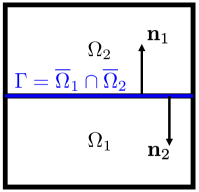
Figure 1: Schematic of a coupled model.

where $\rho_{m}$ is the density $[$\mathrm{kg}\text{\,}{\mathrm{m}}^{-3}$]$; $\mathbf{u}_{m}$ is the velocity vector $[$\mathrm{m}\text{\,}{\mathrm{s}}^{-1}$]$; ${{p}}_{m}$ is the pressure $[$\mathrm{N}\text{\,}{\mathrm{m}}^{-2}$]$; $\rho E_{m}=\rho_{m}e_{m}+\frac{1}{2}\rho_{m}\|\mathbf{u}_{m}\|^{2}$ is the total energy $[$\mathrm{J}\text{\,}{\mathrm{m}}^{-3}$]$; $e_{m}=\frac{{{p}}_{m}}{\rho_{m}(\gamma_{m}-1)}$ is the internal energy $[$\mathrm{J}\text{\,}{\mathrm{kg}}^{-1}$]$; $H_{m}=E_{m}+\frac{{{p}}_{m}}{\rho_{m}}=\frac{a_{m}^{2}}{\gamma_{m}-1}+\frac{1}{2}\|\mathbf{u}_{m}\|^{2}$ is the total specific enthalpy $[$\mathrm{J}\text{\,}{\mathrm{kg}}^{-1}$]$; $\sigma_{m}=\mu_{m}\left(\nabla\mathbf{u}_{m}+\nabla(\mathbf{u}_{m})^{T}-\frac{2}{3}\mathcal{I}\nabla\cdot\mathbf{u}_{m}\right)$ is the viscous stress tensor; $\Pi_{m}=-\kappa_{m}\nabla T_{m}$ is the heat flux; $T_{m}$ is the temperature; $\kappa_{m}=\mu_{m}(c_{p})_{m}Pr_{m}^{-1}$ is the heat conductivity $[$\mathrm{W}\text{\,}{\mathrm{m}}^{-1}\text{\,}{\mathrm{K}}^{-1}$]$; $\mu_{m}$ is the dynamic viscosity $[$\mathrm{Pa}\text{\,}\mathrm{s}$]$; $Pr_{m}$ is Prantl number; $a_{m}=\left(\gamma_{m}\frac{{{p}}_{m}}{\rho_{m}}\right)^{\frac{1}{2}}$ is the sound speed $[$\mathrm{m}\text{\,}{\mathrm{s}}^{-1}$]$ for ideal gas; $\gamma_{m}=\left(\frac{c_{p}}{c_{v}}\right)_{m}$ is the ratio of the specific heats; and $(c_{p})_{m}$ and $(c_{v})_{m}$ are the specific heat capacities at constant pressure and at constant volume $[$\mathrm{J}\text{\,}{\mathrm{kg}}^{-1}\text{\,}{\mathrm{K}}^{-1}$]$, respectively. In a compact form, (1) can be written as

$$\frac{\partial{{\mathbf{q}}_{m}}}{\partial{t}}+\nabla\cdot\mathcal{F}_{m}^{I}({\mathbf{q}}_{m})=\nabla\cdot\mathcal{F}_{m}^{V}({\mathbf{q}}_{m}),$$ (2)

with the conservative variable ${\mathbf{q}}_{m}=(\rho_{m},\rho\mathbf{u}_{m}^{T},\rho E_{m})^{T}$, the inviscid flux tensor $\mathcal{F}_{m}^{I}=(\rho\mathbf{u}_{m},\rho\mathbf{u}_{m}\otimes\mathbf{u}_{m}+\mathcal{I}{{p}}_{m},\rho\mathbf{u}_{m}H_{m})^{T}$, and the viscous flux tensor $\mathcal{F}_{m}^{V}=(0,\sigma_{m},\sigma_{m}\mathbf{u}_{m}-\Pi_{m})^{T}$ for $\Omega_{m}$.

2.1 Interface conditions

The interface $\Gamma$ allows the exchange of heat and horizontal momentum fluxes between the two domains. To implement this, we adapt the rigid-lid assumption used in many oceanography models [38, 39]. In the rigid-lid coupling condition [18, 40], the normal velocity component and normal traction vector at the interface are set to zero, but the continuity of the tangential traction vector and heat flux are enforced:

$${\bf n}_{m}\cdot\mathbf{u}_{m} =0,$$ (3a)

$${\bf n}_{m}\cdot\left(\sigma_{m}{\bf n}_{m}\right) =0,$$ (3b)

$${\bf t}\cdot\left(\sigma_{1}{\bf n}_{1}-\sigma_{2}{\bf n}_{2}\right) =0,$$ (3c)

$${\bf n}_{1}\cdot\Pi_{1}+{\bf n}_{2}\cdot\Pi_{2} =0.$$ (3d)

Here, ${\bf n}_{m}$ is the outward unit normal vectors on $\partial\Omega_{m}$ toward the adjacent domain of $\Omega_{m}$, and ${\bf t}$ is the tangent vector on $\Gamma$. In two dimensions, the rigid-lid interface condition (3) is simplified as

$$\hat{w}_{1} =\hat{w}_{2}=0,$$

$$\hat{\sigma}_{1zz} =\hat{\sigma}_{2zz}=0,$$

$$\mu_{1}\frac{\partial{u_{1}}}{\partial{z}} =\mu_{2}\frac{\partial{u_{2}}}{\partial{z}}=:\hat{\sigma}_{xz},$$

$$-\kappa_{1}\frac{\partial{T_{1}}}{\partial{z}} =-\kappa_{2}\frac{\partial{T_{2}}}{\partial{z}}=:\hat{\Pi}_{z},$$

with ${\bf n}_{1}=(0,1)^{T}$, ${\bf n}_{2}=(0,-1)^{T}$ and ${\bf t}=(1,0)^{T}$.

The next question is how to parameterize the physical heat and horizontal momentum fluxes across the interface. According to previous work in [41, 42, 43, 44], the bulk flux approach is widely used, where the physical fluxes are related to the measurable quantities such as wind-ocean current speed and lower air-sea surface temperature. For example, by introducing the bulk coefficients $b_{u}$ and $b_{T}$, we can associate temperature and velocity with the heat and the horizontal momentum fluxes:

$$\hat{\sigma}_{xz}:=b_{u}(u_{2}-u_{1})\text{ and }\hat{\Pi}_{z}:=-b_{T}(T_{2}-T_{1}).$$ (4)

Several forms of the bulk coefficients have been proposed in earlier work [45, 43, 46], but in this study we use the linear bulk coefficients (with constant $\mu_{1}$,$\mu_{2}$,$\kappa_{1}$ and $\kappa_{2}$):

$$b_{u}=\frac{2\mu_{1}\mu_{2}}{{\triangle z}_{2}\mu_{1}+{\triangle z}_{1}\mu_{2}},\text{ and }b_{T}=\frac{2\kappa_{1}\kappa_{2}}{{\triangle z}_{2}\kappa_{1}+{\triangle z}_{1}\kappa_{2}},$$

which come from the finite difference (FD) approximation of heat and horizontal momentum fluxes.

Once we have computed the heat and the momentum fluxes at the interface by using (4), we estimate the isothermal wall boundary states of $u_{w}$ and $T_{w}$ for $\Omega_{1}$ and $\Omega_{2}$, respectively,

$$u_{w_{1}}=u_{1}+\frac{\hat{\sigma}_{xz}{\triangle z}_{1}}{2\mu_{1}}\text{ and }T_{w_{1}}=T_{1}-\frac{\hat{\Pi}_{z}{\triangle z}_{1}}{2\kappa_{1}},$$

$$u_{w_{2}}=u_{2}-\frac{\hat{\sigma}_{xz}{\triangle z}_{2}}{2\mu_{2}}\text{ and }T_{w_{2}}=T_{2}+\frac{\hat{\Pi}_{z}{\triangle z}_{2}}{2\kappa_{2}},$$

by using FD approximation. Then, we apply the isothermal wall boundary treatment [47] to the interface.

2.2 Nondimensionalization

By the nondimensional variables,

$$\rho^{*}_{m}=\frac{\rho_{m}}{\rho_{r}},{{p}}^{*}_{m}=\frac{{{p}}_{m}}{\rho_{r}u_{r}^{2}},\mathbf{u}^{*}_{m}=\frac{\mathbf{u}_{m}}{u_{r}},x^{*}=\frac{x}{L},t^{*}=\frac{t}{L/u_{r}},\mu^{*}_{m}=\frac{\mu_{m}}{\mu_{r}},\text{ and }T^{*}_{m}=\frac{T_{m}}{T_{r}},$$

we rewrite the governing equation (1) as

$$\frac{\partial{\rho_{m}^{*}}}{\partial{t^{*}}}+\nabla^{*}\cdot\left(\rho\mathbf{u}_{m}^{*}\right) =0,$$ (5a)

$$\frac{\partial{\rho\mathbf{u}_{m}^{*}}}{\partial{t^{*}}}+\nabla^{*}\cdot\left(\rho\mathbf{u}_{m}^{*}\otimes\mathbf{u}_{m}^{*}+\mathcal{I}{{p}}_{m}^{*}\right) =\nabla^{*}\cdot\sigma_{m}^{*},$$ (5b)

$$\frac{\partial{\rho E_{m}^{*}}}{\partial{t^{*}}}+\nabla^{*}\cdot\left(\rho\mathbf{u}_{m}^{*}H_{m}^{*}\right) =\nabla^{*}\cdot(\sigma_{m}^{*}\mathbf{u}_{m}^{*})-\nabla^{*}\cdot\Pi_{m}^{*},$$ (5c)

where $\sigma_{m}^{*}=\tilde{\mu}_{m}\left(\nabla^{*}\mathbf{u}^{*}_{m}+\nabla^{*}(\mathbf{u}^{*}_{m})^{T}-\frac{2}{3}\mathcal{I}\nabla^{*}\cdot\mathbf{u}^{*}_{m}\right)$, $\Pi^{*}_{m}=\frac{\tilde{c}_{p}\tilde{\mu}_{m}}{Pr}\nabla^{*}T^{*}_{m}$, $\nabla^{*}=\frac{1}{L}\nabla$, $\tilde{\mu}_{m}:=\frac{\mu^{*}_{m}}{Re_{r}}$, $Re_{r}:=\frac{\rho_{r}u_{r}L}{\mu_{r}}$ and $\tilde{c}_{p}:=\frac{T_{r}c_{p}}{u_{r}^{2}}$.

We take $\rho_{r}=\rho_{\infty_{2}}$, $\mu_{r}=\mu_{\infty_{2}}$, $T_{r}=T_{\infty_{2}}$, and the speed of sound as a reference velocity, $u_{r}=a_{\infty_{2}}=\sqrt{\gamma RT_{\infty_{2}}}$. The normalized equation of state (EOS) for an ideal gas is ${{p}}^{*}_{m}=\gamma^{-1}\rho^{*}_{m}T^{*}_{m}=\rho^{*}_{m}e^{*}_{m}(\gamma-1)$.

In this study, we use the nondimensionalized form (5), and we omit the superscript ($*$) hereafter.

2.3 Finite volume discretization

We denote by $\Omega_{m_{h}}:=\cup_{\ell=1}^{N_{E_{m}}}K_{m_{\ell}}$ the mesh containing a finite collection of non-overlapping elements, $K_{m_{\ell}}$, that partition $\Omega_{m}$. For example, in a two-dimensional Cartesian coordinates system, we have ${N_{E_{m}}}={N_{xe_{m}}}\times{N_{ze_{m}}}$. For clarity, we abbreviate the subscript $m$ in this section.

Integrating (2) over elements, applying the divergence theorem, and introducing a numerical flux, ${\bf n}\cdot\mathcal{F}^{*}$, we obtain a cell-centered FV scheme for the $\ell$ element,

$$\frac{d{\overline{{\mathbf{q}}}_{\ell}}}{d{t}}=-\frac{1}{\left|K_{\ell}\right|}\int_{{\partial K}_{\ell}}{\bf n}\cdot\mathcal{F}^{*}d{\partial K}=-\frac{1}{\left|K_{\ell}\right|}\sum_{f\in{\partial K}_{\ell}}\int_{f}{\bf n}\cdot\mathcal{F}^{*}df,$$ (6)

where ${\bf n}$ is the outward unit normal vector on the boundary ${\partial K}$ of the element $K$, $f$ is the elemental face of ${\partial K}$, $\overline{{\mathbf{q}}}_{\ell}=\left|K_{\ell}\right|^{-1}\int_{K_{\ell}}\frac{d{{\mathbf{q}}}}{d{t}}dK$ is the average state variable in $K_{\ell}$, and $\left|K_{\ell}\right|$ is the Lebesgue measure of element $K_{\ell}$.

The numerical flux $\mathcal{F}^{*}=\mathcal{F}^{I^{*}}-\mathcal{F}^{V^{*}}$ is composed of two parts: inviscid and viscous. For the inviscid part, we employ the upwind flux based on Roe’s approximation, [48]:

$${\bf n}\cdot\mathcal{F}^{I^{*}} =\frac{1}{2}\left(\mathcal{F}^{I}({\mathbf{q}}^{l})+\mathcal{F}^{I}({\mathbf{q}}^{r})\right)\cdot{\bf n}+\frac{|A|}{2}\left({\mathbf{q}}^{r}{\bf n}^{r}+{\mathbf{q}}^{l}{\bf n}^{l}\right)\cdot{\bf n},$$

where ${\mathbf{q}}^{l}$ and ${\mathbf{q}}^{r}$ are the reconstructed values from the left and the right sides of the elemental face $f$; $|A|:=\mathcal{R}|\Lambda|\mathcal{R}^{-1}$; $A:=\frac{\partial{\mathcal{F}^{I}\cdot{\bf n}}}{\partial{{\mathbf{q}}}}=\mathcal{R}\Lambda\mathcal{R}^{-1}$ is the flux Jacobian; and $\mathcal{R}$ and $\Lambda$ are eigenvectors and eigenvalues of the flux Jacobian (details can be found in [49]). For the viscous part, inspired by [50], we first compute the common velocity ($\hat{\mathbf{u}}$), common velocity gradient ($\widehat{\nabla\mathbf{u}}$), and common temperature gradient ($\widehat{\nabla T}$) at the elemental face $f$ and then evaluate the viscous flux

$${\bf n}\cdot\mathcal{F}^{V^{*}}:={\bf n}\cdot\mathcal{F}^{V}\left(\hat{\mathbf{u}},\widehat{\nabla\mathbf{u}},\widehat{\nabla T}\right).$$

Two-dimensional $(x,z)$ uniform grid

With a two-dimensional uniform mesh, (6) for the $\ell=(i,j)$ element becomes

$$\frac{d{\overline{{\mathbf{q}}}_{(i,j)}}}{d{t}}=-\frac{1}{{\triangle x}}\left({{\bf F}^{*}}_{({i+\frac{1}{2}},j)}-{{\bf F}^{*}}_{({i-\frac{1}{2}},j)}\right)-\frac{1}{{\triangle z}}\left({{\bf G}^{*}}_{(i,{j+\frac{1}{2}})}-{{\bf G}^{*}}_{(i,{j-\frac{1}{2}})}\right),$$ (7)

where ${{\bf F}^{*}}={\bf F}^{I^{*}}-{\bf F}^{V^{*}}$, ${{\bf G}^{*}}=\mathbf{G}^{I^{*}}-\mathbf{G}^{V^{*}}$, ${\bf F}^{I^{*}}=\left(\rho u,\rho uu+{{p}},\rho uw,\rho uH\right)^{*^{T}}$, ${{\bf G}^{*}}^{I^{*}}=\left(\rho w,\rho wu,\rho ww+{{p}},\rho wH\right)^{*^{T}}$, ${\bf F}^{V^{*}}=\left(0,\sigma_{xx},\sigma_{xz},\sigma_{xx}u+\sigma_{xz}w-\Pi_{x}\right)^{*^{T}}$, and ${{\bf G}^{*}}^{V^{*}}=\left(0,\sigma_{zx},\sigma_{zz},\sigma_{zx}u+\sigma_{zz}w-\Pi_{z}\right)^{*^{T}}$.

For the cell-centered second-order FV, we compute the numerical fluxes in (7) using linearly reconstructed variables. Since each element has only cell-averaged values, the reconstruction requires information from adjacent elements. For the inviscid flux (${\bf F}^{I^{*}}\text{ and }\mathbf{G}^{I^{*}}$), we compute the cell-centered gradients $\overline{\nabla{\mathbf{q}}}$ using the least-square (LS) scheme [51]. With the gradients, the left and the right conserved variables (${\mathbf{q}}^{l}$ and ${\mathbf{q}}^{r}$) are obtained by

$${\mathbf{q}}_{(i+\frac{1}{2},j)}^{l} =\overline{{\mathbf{q}}}_{(i,j)}+\overline{\frac{\partial{{\mathbf{q}}}}{\partial{x}}}_{(i,j)}\frac{{\triangle x}}{2},\quad{\mathbf{q}}_{(i+\frac{1}{2},j)}^{r}=\overline{{\mathbf{q}}}_{(i+1,j)}-\overline{\frac{\partial{{\mathbf{q}}}}{\partial{x}}}_{(i+1,j)}\frac{{\triangle x}}{2}$$

at the $x$-face of $(i+\frac{1}{2},j)$ and

$${\mathbf{q}}_{(i,j+\frac{1}{2})}^{l} =\overline{{\mathbf{q}}}_{(i,j)}+\overline{\frac{\partial{{\mathbf{q}}}}{\partial{z}}}_{(i,j)}\frac{{\triangle z}}{2},\quad{\mathbf{q}}_{(i,j+\frac{1}{2})}^{r}=\overline{{\mathbf{q}}}_{(i,j+1)}-\overline{\frac{\partial{{\mathbf{q}}}}{\partial{z}}}_{(i,j+1)}\frac{{\triangle z}}{2}$$

at the $z$-face of $(i,j+\frac{1}{2})$.

For the viscous flux (${\bf F}^{V^{*}}\text{ and }\mathbf{G}^{V^{*}}$), we compute the cell-centered gradients of velocity and temperature ($\overline{\nabla\mathbf{u}}$ and $\overline{\nabla T}$) by using the LS scheme, and we compute the common velocity of $\hat{\mathbf{u}}$,

$$\hat{\mathbf{u}}_{(i+\frac{1}{2},j)}=\frac{1}{2}\left(\overline{\mathbf{u}}_{(i,j)}+\overline{\mathbf{u}}_{(i+1,j)}\right),\quad\hat{\mathbf{u}}_{(i,j+\frac{1}{2})}=\frac{1}{2}\left(\overline{\mathbf{u}}_{(i,j)}+\overline{\mathbf{u}}_{(i,j+1)}\right),$$

by taking an arithmetic average. As for the common gradients of $\widehat{\nabla\mathbf{u}}$ and $\widehat{\nabla T}$, we obtain normal gradients by finite difference approximation

$$\widehat{\frac{\partial{u}}{\partial{x}}}_{(i+\frac{1}{2},j)} =\frac{1}{{\triangle x}}\left(\overline{u}_{(i+1,j)}-\overline{u}_{(i,j)}\right), \widehat{\frac{\partial{u}}{\partial{z}}}_{(i,j+\frac{1}{2})} =\frac{1}{{\triangle z}}\left(\overline{u}_{(i,j+1)}-\overline{u}_{(i,j)}\right),$$

$$\widehat{\frac{\partial{w}}{\partial{x}}}_{(i+\frac{1}{2},j)} =\frac{1}{{\triangle x}}\left(\overline{w}_{(i+1,j)}-\overline{w}_{(i,j)}\right), \widehat{\frac{\partial{w}}{\partial{z}}}_{(i,j+\frac{1}{2})} =\frac{1}{{\triangle z}}\left(\overline{w}_{(i,j+1)}-\overline{w}_{(i,j)}\right),$$

$$\widehat{\frac{\partial{T}}{\partial{x}}}_{(i+\frac{1}{2},j)} =\frac{1}{{\triangle x}}\left(\overline{T}_{(i+1,j)}-\overline{T}_{(i,j)}\right), \widehat{\frac{\partial{T}}{\partial{z}}}_{(i,j+\frac{1}{2})} =\frac{1}{{\triangle z}}\left(\overline{T}_{(i,j+1)}-\overline{T}_{(i,j)}\right),$$

and tangential gradients by averaging two adjacent cell-centered gradients,

$$\widehat{\frac{\partial{u}}{\partial{z}}}_{(i+\frac{1}{2},j)} =\frac{1}{2}\left(\overline{\frac{\partial{u}}{\partial{z}}}_{(i,j)}+\overline{\frac{\partial{u}}{\partial{z}}}_{(i+1,j)}\right), \widehat{\frac{\partial{u}}{\partial{x}}}_{(i,j+\frac{1}{2})} =\frac{1}{2}\left(\overline{\frac{\partial{u}}{\partial{z}}}_{(i,j)}+\overline{\frac{\partial{u}}{\partial{z}}}_{(i,j+1)}\right),$$

$$\widehat{\frac{\partial{w}}{\partial{x}}}_{(i,j+\frac{1}{2})} =\frac{1}{2}\left(\overline{\frac{\partial{w}}{\partial{z}}}_{(i,j)}+\overline{\frac{\partial{w}}{\partial{z}}}_{(i,j+1)}\right), \widehat{\frac{\partial{w}}{\partial{z}}}_{(i+\frac{1}{2},j)} =\frac{1}{2}\left(\overline{\frac{\partial{w}}{\partial{z}}}_{(i,j)}+\overline{\frac{\partial{w}}{\partial{z}}}_{(i+1,j)}\right),$$

$$\widehat{\frac{\partial{T}}{\partial{x}}}_{(i,j+\frac{1}{2})} =\frac{1}{2}\left(\overline{\frac{\partial{T}}{\partial{z}}}_{(i,j)}+\overline{\frac{\partial{T}}{\partial{z}}}_{(i,j+1)}\right), \widehat{\frac{\partial{T}}{\partial{z}}}_{(i+\frac{1}{2},j)} =\frac{1}{2}\left(\overline{\frac{\partial{T}}{\partial{z}}}_{(i,j)}+\overline{\frac{\partial{T}}{\partial{z}}}_{(i+1,j)}\right).$$

3 IMEX coupling framework

In this section we introduce IMEX coupling methods in which we treat one model implicitly and the other model explicitly. IMEX coupling schemes naturally support two-way coupling for all stages. This means that at every time stage the continuity of the heat and the horizontal momentum fluxes is ensured by construction. For example, at the $i$th stage,

$$\hat{\sigma}_{xz}^{(i)}=b_{u}(u^{(i)}_{2}-u^{(i)}_{1}),\text{ and }\hat{\Pi}_{z}^{(i)}=-b_{T}(T^{(i)}_{2}-T^{(i)}_{1}).$$

We denote two-way coupling at every stage as tight coupling (TC), which is represented by double arrows in Figure 2(a).

With two domains that exhibit different stiffness properties, IMEX methods represent a suitable alternative to monolithic implicit methods by alleviating the cost of applying an implicit method on the less stiff partition. Moreover, the IMEX tight coupling approach supports a high-order solution in time, reduces the computational cost arising from an implicit monolithic approach, and allows a large timestep size compared with that of a fully explicit coupling approach. However, the tight coupling requires frequent communications between the two models across the interface and also sequentially advances each model (e.g., runs the atmosphere model first and then updates the ocean model). Furthermore, each model is advanced with the same timestep size.

To confer more timestepping granularity, one may consider loosening the tight coupling so that each model can march with a different timestep size [53, 54, 55, 56, 57], for example, ${\triangle t}_{ocn}=N_{s}{\triangle t}_{atm}$, or can run simultaneously. Therefore, we consider two loose coupling (LC) schemes: concurrent and sequential.

For concurrent coupling (CC), the two models run simultaneously by two-way coupling at each colocated time level. For example, the atmospheric model and ocean model are two-way coupled at every ${\triangle t}_{ocn}=2{\triangle t}_{atm}$ in Figure 2(b). For sequential coupling (SC), we run one model first and then advance the other model. For example, as can be seen in Figure 2(c), after two-way coupling has occurred at the beginning of each colocated time level, we advance the ocean model first while freezing the interface data. Then we update the atmospheric model by providing the updated solution from the ocean model at each stage.

Obviously, in both the concurrent and the sequential coupling approaches, the heat and the horizontal momentum fluxes are not always continuous at every stage in general. For example, at the $i(>1)$th stage,

$$\hat{\sigma}_{1xz}^{(i)}=b_{u}(u^{(i)}_{2}-u^{n}_{1}) \neq b_{u}(u^{n}_{2}-u^{(i)}_{1})=\hat{\sigma}_{2xz}^{(i)},$$

$$\hat{\Pi}_{1z}^{(i)}=-b_{T}(T^{(i)}_{2}-T^{n}_{1}) \neq-b_{T}(T^{n}_{2}-T^{(i)}_{1})=\hat{\Pi}_{2z}^{(i)}$$

for concurrent coupling, and

$$\hat{\sigma}_{1xz}^{(i)}=b_{u}(u^{(i)}_{1}-u^{(i)}_{2}) \neq b_{u}(u^{n}_{1}-u^{(i)}_{2})=\hat{\sigma}_{2xz}^{(i)},$$

$$\hat{\Pi}_{1z}^{(i)}=-b_{T}(T^{(i)}_{1}-T^{(i)}_{2}) \neq-b_{T}(T^{n}_{1}-T^{(i)}_{2})=\hat{\Pi}_{2z}^{(i)}$$

for sequential coupling. The interface data is not always available during the time level. interval. Consequently, compared with tight coupling, loose coupling leads to a degraded rate of convergence in time but can increase the solution accuracy when dynamics rapidly changes because of substeps (see ARK3 in Table 6).

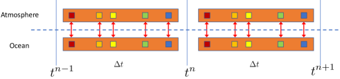
(a) Tight coupling (TC)

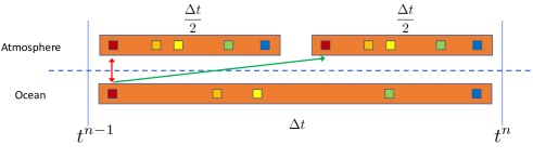
(b) Concurrent coupling with two substeps (CC2)

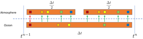
(c) Sequential coupling with two substeps (SC2)

Figure 2: Coupling diagrams: (a) tight coupling, (b) concurrent with two substeps (CC2), and (c) sequential coupling with two substeps (SC2). Five-time stages are illustrated by small ( ,  ,  ,  , and  ) boxes. The single (green) and the double (red) arrows describe one-way and two-way couplings, respectively. For tight coupling, two-way coupling occurs at every stage, whereas for loose coupling, two-way coupling is only performed at each colocated time level. After the colocated time level, for concurrent coupling, the two models run simultaneously without updating interface data; and for sequential coupling, the ocean model run first while freezing the interface data, and then the atmospheric model is marched by providing the updated solution from the ocean model at each stage.

Without loss of generality, in this study we refer to the model on $\Omega_{1}$ as the ocean model and to the model on $\Omega_{2}$ as the atmospheric model for convenience. For TC, we treat the ocean implicitly and the atmosphere explicitly within the IMEX coupling framework. For LC, we advance the ocean model using IMEX methods but march the atmospheric model explicitly using the explicit part of the IMEX methods. The interface is treated explicitly. Detailed algorithms are shown in the following subsections.

3.1 IMEX-RK tight coupling methods

We discretize (5) by using the FV method in (7), which yields the following semi-discretized coupled systems,

$$\frac{d{{\mathbf{q}}_{1}}}{d{t}} =\mathbf{R}_{1}({\mathbf{q}}_{1},{\mathbf{q}}_{2})\text{ on }\Omega_{1},$$ (8a)

$$\frac{d{{\mathbf{q}}_{2}}}{d{t}} =\mathbf{R}_{2}({\mathbf{q}}_{1},{\mathbf{q}}_{2})\text{ on }\Omega_{2},$$ (8b)

with ${\mathbf{q}}_{m}=({\mathbf{q}}_{m_{1}},{\mathbf{q}}_{m_{2}},\cdots,{\mathbf{q}}_{m_{N_{E_{m}}}})^{T}$ and $\mathbf{R}_{m}=(\mathbf{R}_{m_{1}},\mathbf{R}_{m_{2}},\cdots,\mathbf{R}_{m_{N_{E_{m}}}})^{T}$ for $m=1,2$. Here, we omit the overline (which stands for cell-averaged quantity) for brevity.

Under the assumption that the ocean model is stiffer than the atmospheric model, we cast (8) into $s$-stage IMEX-RK methods [22, 23, 25, 32],

$${\bf Q}^{(i)} ={\bf Q}^{n}+\triangle t\sum_{j=1}^{i-1}a_{ij}\mathbf{f}_{j}+\triangle t\sum_{j=1}^{i}\tilde{a}_{ij}\mathbf{g}_{j},\quad i=1,\ldots,s,$$ (9a)

$${\mathbf{q}}^{n+1} ={\mathbf{q}}^{n}+\triangle t\sum_{i=1}^{s}b_{i}\mathbf{f}_{i}+\triangle t\sum_{i=1}^{s}\tilde{b}_{i}\mathbf{g}_{i},$$ (9b)

where ${\mathbf{q}}=({\mathbf{q}}_{1},{\mathbf{q}}_{2})^{T}$, ${\bf Q}=({\bf Q}_{1},{\bf Q}_{2})^{T}$, $\mathbf{f}=(0,\mathbf{R}_{2})^{T}$, $\mathbf{g}=(\mathbf{R}_{1},0)^{T}$, $\mathbf{f}_{i}=\mathbf{f}\left(t^{n}+c_{i}\triangle t,{\bf Q}^{(i)}\right)$, $\mathbf{g}_{i}=\mathbf{g}\left(t^{n}+\tilde{c}_{i}\triangle t,{\bf Q}^{(i)}\right)$, ${\mathbf{q}}^{n}={\mathbf{q}}(t^{n})$; ${\bf Q}^{(i)}$ is the $i$th intermediate state; and $\triangle t$ is the timestep size. The scalar coefficients $a_{ij}$, $\tilde{a}_{ij}$, $b_{i}$, $\tilde{b}_{i}$, $c_{i}$, and $\tilde{c}_{i}$ determine all the properties of a given IMEX-RK scheme.

The intermediate state ${\bf Q}^{(i)}$ in (9a) is

$$\begin{pmatrix}{\bf Q}_{1}^{(i)}\\ {\bf Q}_{2}^{(i)}\end{pmatrix}-\triangle t\tilde{a}_{ii}\begin{pmatrix}\mathbf{R}_{1}({\bf Q}^{(i)})\\ 0\end{pmatrix} =\begin{pmatrix}{\mathbf{q}}_{1}^{n}\\ {\mathbf{q}}_{2}^{n}\end{pmatrix}+\triangle t\sum_{j=1}^{i-1}\begin{pmatrix}a_{ij}\mathbf{R}_{1j}\\ \tilde{a}_{ij}\mathbf{R}_{2j}\end{pmatrix}=:\begin{pmatrix}\check{{\bf Q}}_{1}\\ \check{{\bf Q}}_{2}\end{pmatrix}$$ (10)

with $\mathbf{R}_{ij}:=\mathbf{R}_{i}({\bf Q}^{(j)})$. Thanks to the semi-implicit structure, we explicitly update ${\bf Q}_{2}^{(i)}$ from the second row in (10) and then solve for ${\bf Q}_{1}^{(i)}$ implicitly. The next timestep solution is obtained by (9b) after solving for all the intermediate stages:

$${{\mathbf{q}}}_{1}^{n+1} ={\mathbf{q}}_{1}^{n}+\triangle t\sum_{i=1}^{s}\tilde{b}_{i}\mathbf{R}_{1i},$$ (11a)

$${{\mathbf{q}}}_{2}^{n+1} ={\mathbf{q}}_{2}^{n}+\triangle t\sum_{i=1}^{s}b_{i}\mathbf{R}_{2i}.$$ (11b)

These steps are summarized in Algorithm 1. Note that at the time of computing the right-hand sides, $\mathbf{R}_{1}$ and $\mathbf{R}_{2}$, both the solution ${\bf Q}_{1}$ and the solution ${\bf Q}_{2}$ are available at the same time; hence, the bulk fluxes in (4) are conservative at each stage.

0:  Given solution state ${\mathbf{q}}^{n}$, compute its next solution state ${\mathbf{q}}^{n+1}$ under the assumption that $\mathbf{R}_{1}$ is stiffer than $\mathbf{R}_{2}$. Let $\mathbf{R}_{1i}:=\mathbf{R}_{1}({\bf Q}_{1}^{(i)},{\bf Q}_{2}^{(i)})$ and $\mathbf{R}_{2i}:=\mathbf{R}_{2}({\bf Q}_{1}^{(i)},{\bf Q}_{2}^{(i)})$.

1:  for $i=1$ to $s$ do

2:     if $\tilde{a}_{ii}=0$ then

3:        ${\bf Q}_{1}^{(i)}\leftarrow{\mathbf{q}}_{1}^{n}$

4:        ${\bf Q}_{2}^{(i)}\leftarrow{\mathbf{q}}_{2}^{n}$

5:     else

6:        ${{\bf Q}}_{2}^{(i)}\leftarrow{\mathbf{q}}_{2}^{n}+\triangle t\sum_{j=1}^{i-1}a_{ij}\mathbf{R}_{2j}$

7:        $\check{{\bf Q}}_{1}^{(i)}\leftarrow{\mathbf{q}}_{1}^{n}+\triangle t\sum_{j=1}^{i-1}\tilde{a}_{ij}\mathbf{R}_{1j}$

8:        Solve for ${\bf Q}_{1}^{(i)}$ according to (10)

9:     end if

10:     Send/Receive interface information from $\Omega_{1}$ to $\Omega_{2}$, vice versa.

11:     Compute stage right-hand sides, $\mathbf{R}_{1i}$ and $\mathbf{R}_{2i}$

12:  end for

13:  ${{\mathbf{q}}}_{1}^{n+1}\leftarrow{\mathbf{q}}_{1}^{n}+\triangle t\sum_{i=1}^{s}\tilde{b}_{i}\mathbf{R}_{1i}$

14:  ${{\mathbf{q}}}_{2}^{n+1}\leftarrow{\mathbf{q}}_{2}^{n}+\triangle t\sum_{i=1}^{s}{b}_{i}\mathbf{R}_{2i}$

Algorithm 1 Partitioned IMEX-RK Coupling

To avoid nonlinear solves for ${\bf Q}_{1}$, we can linearize $\mathbf{R}_{1}$ and use the same IMEX methods [32, 29] to solve only linear systems at each stage. We do so by choosing $\mathbf{L}$, a linear operator containing stiff components of $\mathbf{R}_{1}$, and then constructing a term by subtracting $\mathbf{L}$ from $\mathbf{R}_{1}$ in the hope that this term is nonstiff, that is, ${\bf N}:=\mathbf{R}_{1}-\mathbf{L}$. By taking $\mathbf{f}=({\bf N},\mathbf{R}_{2})^{T}$ and $\mathbf{g}=(\mathbf{L},0)^{T}$, the intermediate state ${\bf Q}^{(i)}$ in (9a) becomes

$$\begin{pmatrix}{\bf Q}_{1}^{(i)}\\ {\bf Q}_{2}^{(i)}\end{pmatrix}-\triangle t\tilde{a}_{ii}\begin{pmatrix}\mathbf{L}({\bf Q}^{(i)})\\ 0\end{pmatrix} =\begin{pmatrix}{\mathbf{q}}_{1}^{n}\\ {\mathbf{q}}_{2}^{n}\end{pmatrix}+\triangle t\sum_{j=1}^{i-1}\begin{pmatrix}a_{ij}{\bf N}_{j}+\tilde{a}_{ij}\mathbf{L}_{j}\\ a_{ij}\mathbf{R}_{2j}\end{pmatrix}$$ (12)

with $\mathbf{L}_{j}:=\mathbf{L}({\bf Q}^{(j)})$ and ${\bf N}_{j}:=\mathbf{R}_{1j}-\mathbf{L}_{j}$. This form requires only one linear solve to update ${\bf Q}_{1}^{(i)}$. We update the next timestep solution as follows:

$${{\mathbf{q}}}_{1}^{n+1} ={\mathbf{q}}_{1}^{n}+\triangle t\sum_{i=1}^{s}\left(b_{i}{\bf N}_{i}+\tilde{b}_{i}\mathbf{L}_{i}\right),$$ (13a)

$${{\mathbf{q}}}_{2}^{n+1} ={\mathbf{q}}_{2}^{n}+\triangle t\sum_{i=1}^{s}b_{i}\mathbf{R}_{2i}.$$ (13b)

The algorithm is summarized in Algorithm 2.

0:  Given solution state ${\mathbf{q}}^{n}$, compute its next solution state ${\mathbf{q}}^{n+1}$ under the assumption that $\mathbf{R}_{1}$ is stiffer than $\mathbf{R}_{2}$, and $\mathbf{L}$ contains stiff components of $\mathbf{R}_{1}$. Let $\mathbf{R}_{1i}:=\mathbf{R}_{1}({\bf Q}_{1}^{(i)},{\bf Q}_{2}^{(i)})$, $\mathbf{R}_{2i}:=\mathbf{R}_{2}({\bf Q}_{1}^{(i)},{\bf Q}_{2}^{(i)})$, $\mathbf{L}_{i}:=\mathbf{L}({\bf Q}_{1}^{(i)},{\bf Q}_{2}^{(i)})$, and ${\bf N}_{i}=\mathbf{R}_{1i}-\mathbf{L}_{i}$.

1:  for $i=1$ to $s$ do

2:     if $\tilde{a}_{ii}=0$ then

3:        ${\bf Q}_{1}^{(i)}\leftarrow{\mathbf{q}}_{1}^{n}$

4:        ${\bf Q}_{2}^{(i)}\leftarrow{\mathbf{q}}_{2}^{n}$

5:     else

6:        ${{\bf Q}}_{2}^{(i)}\leftarrow{\mathbf{q}}_{2}^{n}+\triangle t\sum_{j=1}^{i-1}a_{ij}\mathbf{R}_{2j}$

7:        $\check{{\bf Q}}_{1}^{(i)}\leftarrow{\mathbf{q}}_{1}^{n}+\triangle t\sum_{j=1}^{i-1}\left(a_{ij}{\bf N}_{j}+\tilde{a}_{ij}\mathbf{L}_{j}\right)$

8:        Linear solve for ${\bf Q}_{1}^{(i)}$

9:     end if

10:     Send/Receive interface information from $\Omega_{1}$ to $\Omega_{2}$, vice versa.

11:     Compute stage right-hand-sides, $\mathbf{R}_{2i}$, ${\bf N}_{i}$ and $\mathbf{L}_{i}$

12:  end for

13:  ${{\mathbf{q}}}_{1}^{n+1}\leftarrow{\mathbf{q}}_{1}^{n}+\triangle t\sum_{i=1}^{s}\left(b_{i}{\bf N}_{i}+\tilde{b}_{i}\mathbf{L}_{i}\right)$

14:  ${{\mathbf{q}}}_{2}^{n+1}\leftarrow{\mathbf{q}}_{2}^{n}+\triangle t\sum_{i=1}^{s}b_{i}\mathbf{R}_{2i}$

Algorithm 2 Partitioned IMEX-RK Coupling with Linearized Stiff Flux

3.1.1 The linear operator $\mathbf{L}$

We construct a stiff linear operator $\mathbf{L}$ so that the numerical stiffness of ${\bf N}(=\mathbf{R}_{1}-\mathbf{L})$ is relaxed. Since the Jacobian of the right-hand side $\frac{\partial{\mathbf{R}_{1}}}{\partial{{\mathbf{q}}}}$ contains the stiffness, a linear operator can be chosen as an approximation of the Jacobian to some degree. For example, with a two-dimensional uniform mesh, we can define the linear operator for $(i,j)$ element by

$$\mathbf{L}(\tilde{{\mathbf{q}}},{\mathbf{q}})_{(i,j)}:=-\frac{1}{{\triangle x}}\left({{\bf F}^{*}}_{L,({i+\frac{1}{2}},j)}-{{\bf F}^{*}}_{L,({i-\frac{1}{2}},j)}\right)-\frac{1}{{\triangle z}}\left({{\bf G}^{*}}_{L,(i,{j+\frac{1}{2}})}-{{\bf G}^{*}}_{L,(i,{j-\frac{1}{2}})}\right),$$ (14)

where $\tilde{{\mathbf{q}}}$ is the reference state and ${{\bf F}^{*}}_{L}:=\frac{\partial{{{\bf F}^{*}}}}{\partial{{\mathbf{q}}}}\bigg{|}_{\tilde{{\mathbf{q}}}}{\mathbf{q}}$ and ${{\bf G}^{*}}_{L}:=\frac{\partial{{{\bf G}^{*}}}}{\partial{{\mathbf{q}}}}\bigg{|}_{\tilde{{\mathbf{q}}}}{\mathbf{q}}$ are $x$ and $z$ directional linear fluxes.

If the inviscid part is stiffer than the viscous part, then the linearized viscous part can be dropped from (14), leading to

$$\mathbf{L}^{I}(\tilde{{\mathbf{q}}},{\mathbf{q}})_{(i,j)}:=-\frac{1}{{\triangle x}}\left({\bf F}^{I^{*}}_{L,({i+\frac{1}{2}},j)}-{\bf F}^{I^{*}}_{L,({i-\frac{1}{2}},j)}\right)-\frac{1}{{\triangle z}}\left(\mathbf{G}^{I^{*}}_{L,(i,{j+\frac{1}{2}})}-\mathbf{G}^{I^{*}}_{L,(i,{j-\frac{1}{2}})}\right)$$ (15)

with ${\bf F}^{I^{*}}_{L}:=\frac{\partial{{\bf F}^{I^{*}}}}{\partial{{\mathbf{q}}}}\bigg{|}_{\tilde{{\mathbf{q}}}}{\mathbf{q}}$ and $\mathbf{G}^{I^{*}}_{L}:=\frac{\partial{\mathbf{G}^{I^{*}}}}{\partial{{\mathbf{q}}}}\bigg{|}_{\tilde{{\mathbf{q}}}}{\mathbf{q}}$.

From a computational point of view, both (14) and (15) can be expensive without a proper preconditioner because of their large number of degrees of freedom and global communication in $(x,z)$ domains. To reduce the computational cost, we can adapt the dimensional splitting approach, used in horizontally explicit and vertically implicit (HEVI) methods [32, 58, 33]. For HEVI, we define the linear operator by

$$\mathbf{L}^{z}(\tilde{{\mathbf{q}}},{\mathbf{q}})_{(i,j)}:=-\frac{1}{{\triangle z}}\left(\mathbf{G}^{I^{*}}_{L,(i,{j+\frac{1}{2}})}-\mathbf{G}^{I^{*}}_{L,(i,{j-\frac{1}{2}})}\right)$$ (16)

with only the linear inviscid flux in the vertical direction.

3.2 IMEX-RK loose coupling methods

Now we consider a practical situation where there is a fixed time-scale difference between the two domains. For example, the timestep size of the ocean model, ${\triangle t}_{1}$, is $N_{s}$ times larger than that of the atmosphere, ${\triangle t}_{2}$, namely, ${\triangle t}_{1}=N_{s}{\triangle t}_{2}$. We let ${\mathbf{q}}^{n+1}_{1}$ and ${\mathbf{q}}^{n+\frac{k}{N_{s}}}_{2}$ be numerical approximations of ${\mathbf{q}}_{1}(t^{n}+{\triangle t}_{1})$ and ${\mathbf{q}}_{2}(t^{n}+k{\triangle t}_{2})$, respectively.

We advance the ocean model by using $s$-stage IMEX-RK schemes, which can also provide the dense output formulas of order $p^{*}$ [25],

$${\bf Q}^{*}(t^{n}+\theta{\triangle t}):={\mathbf{q}}^{n}+{\triangle t}\sum_{i=1}^{s}B^{*}_{i}(\theta){\bf N}_{i}+\widehat{B}^{*}_{i}(\theta)\mathbf{L}_{i}.$$

Here, ${\bf N}_{i}:={\bf N}(t^{n}+c_{i}{\triangle t},Q^{(i)})$, $\mathbf{L}_{i}:=\mathbf{L}(t^{n}+\tilde{c}_{i}{\triangle t},Q^{(i)})$, $\theta\in[0,1]$, $B^{*}_{i}(\theta)=\sum_{j=1}^{p^{*}}b^{*}_{ij}\theta^{j}$, and $b^{*}_{ij}$ is a matrix of coefficients of size $s\times p^{*}$. With the ARK schemes satisfying $\widehat{B}^{*}_{i}(\theta)=B^{*}_{i}(\theta)$ and $\tilde{c}_{i}=c_{i}$, we have the time polynomial for ARK methods,[32]

$${\bf Q}^{*}(t^{n}+\theta{\triangle t}):={\mathbf{q}}^{n}+{\triangle t}\sum_{i=1}^{s}B^{*}_{i}(\theta)\mathbf{R}_{i}\,.$$ (17)

For sequential coupling (SC), we integrate the ocean model using $s$-stage IMEX-RK and the atmospheric model using s-stage RK (explicit part of IMEX-RK). We construct the time polynomial (17) and evaluate ${\bf Q}^{*}$ at every RK stage during the substeps. For example, with two substeps, ${\bf Q}^{*}$ is interpolated at $t^{n}+(k-1+c_{i}){\triangle t}_{2}$ for $k=1,2$ and $i=1,2\cdots,s$. For concurrent coupling (CC), we simply take ${\bf Q}^{*}(t^{n}+\theta{\triangle t})={\mathbf{q}}^{n}$. The algorithm is summarized in Algorithm 3.

We call the sequential and the concurrent couplings with $N_{s}$ substeps by SC$\{N_{s}\}$ and CC$\{N_{s}\}$, respectively.

0:  Given solution state ${\mathbf{q}}^{n}_{1}$ and ${\mathbf{q}}^{n}_{2}$, compute their next solution states ${\mathbf{q}}^{n+1}_{1}$ and ${\mathbf{q}}^{n+1}_{2}$ under the assumption of ${\triangle t}_{1}=N_{s}{\triangle t}_{2}$ and $\mathbf{L}$ containing stiff components of $\mathbf{R}_{1}$. Let $\mathbf{R}_{1i}:=\mathbf{R}_{1}({\bf Q}_{1}^{(i)},{\mathbf{q}}^{n}_{2})$, $\mathbf{R}_{2i}:=\mathbf{R}_{2}({\bf Q}_{1}^{*,(i)},{\bf Q}_{2}^{(i)})$, ${\bf Q}_{1}^{*,(i)}:={\bf Q}_{1}^{*}(t^{n}+(k-1+c_{i}){\triangle t}_{2})$, $\mathbf{L}_{i}:=\mathbf{L}({\bf Q}_{1}^{(i)},{\mathbf{q}}^{n}_{2})$, and ${\bf N}_{i}=\mathbf{R}_{1i}-\mathbf{L}_{i}$.

1:  Exchange interface information from atmospheric model to ocean model

2:  for $i=1$ to $s$ do

3:     if $\tilde{a}_{ii}=0$ then

4:        ${\bf Q}_{1}^{(i)}\leftarrow{\mathbf{q}}_{1}^{n}$

5:     else

6:        $\check{{\bf Q}}_{1}^{(i)}\leftarrow{\mathbf{q}}_{1}^{n}+\triangle t_{1}\sum_{j=1}^{i-1}\left(a_{ij}{\bf N}_{j}+\tilde{a}_{ij}\mathbf{L}_{j}\right)$

7:        Linear solve for ${\bf Q}_{1}^{(i)}$

8:     end if

9:     Compute stage right-hand sides, i.e., ${\bf N}_{i}$ and $\mathbf{L}_{i}$

10:  end for

11:  ${{\mathbf{q}}}_{1}^{n+1}\leftarrow{\mathbf{q}}_{1}^{n}+\triangle t_{1}\sum_{i=1}^{s}\left(b_{i}{\bf N}_{i}+\tilde{b}_{i}\mathbf{L}_{i}\right)$

12:  for $k=1$ to $N_{s}$ do

13:     for $i=1$ to $s$ do

14:        if $i=1$ then

15:           ${\bf Q}_{2}^{(i)}\leftarrow{\mathbf{q}}_{2}^{n+\frac{k}{N_{s}}}$

16:        else

17:           ${\bf Q}_{2}^{(i)}\leftarrow{\mathbf{q}}_{2}^{n}+\triangle t_{2}\sum_{j=1}^{i-1}a_{ij}\mathbf{R}_{2i}$

18:        end if

19:        Interpolate ${\bf Q}_{1}^{*,(i)}$

20:        Compute stage right-hand sides, $\mathbf{R}_{2i}$

21:     end for

22:     ${{\mathbf{q}}}_{2}^{n+\frac{k}{N_{s}}}\leftarrow{\mathbf{q}}_{2}^{n+\frac{k-1}{N_{s}}}+\triangle t\sum_{i=1}^{s}b_{i}\mathbf{R}_{2i}$

23:  end for

Algorithm 3 IMEX-RK Loose Coupling Methods

3.3 Mass-conserving IMEX-RK coupling

Conservation of mass is the most fundamental conservation property because it is related to many other conservation properties such as tracer and energy. Any imperfection in the conservation of mass will affect long-time integration, which can generate a superficial pressure field via the equation of states and eventually lead to unwanted modes. [59] Thus, we examine the mass conservation property in the IMEX-RK coupling framework.

We define the total mass in $\Omega=\Omega_{1}\cup\Omega_{2}$ by

mass $$=\int_{\Omega_{1}}\rho d\Omega+\int_{\Omega_{2}}\rho d\Omega=\sum_{\ell=1}^{{N_{E_{1}}}}\int_{K_{1_{\ell}}}\rho dK+\sum_{\ell=1}^{{N_{E_{2}}}}\int_{K_{2_{\ell}}}\rho dK$$

$$=\sum_{\ell=1}^{{N_{E_{1}}}}\bar{\rho}_{1_{\ell}}\left|K_{1_{\ell}}\right|+\sum_{\ell=1}^{{N_{E_{2}}}}\bar{\rho}_{2_{\ell}}\left|K_{2_{\ell}}\right|=\text{mass}_{1}+\text{mass}_{2},$$

where $\text{mass}_{m}=\sum_{\ell=1}^{{N_{E_{m}}}}\bar{\rho}_{m_{\ell}}\left|K_{m_{\ell}}\right|$ ; $\bar{\rho}_{m_{\ell}}=\left|K_{m_{\ell}}\right|^{-1}\int_{K_{m_{\ell}}}\rho dK$ is the mean density on $K_{m_{\ell}}$.

Proposition 3.1.

The IMEX-RK coupling methods with $b_{i}=\tilde{b}_{i}$ in (11) and (13) are mass conservative for system (1) with the FV scheme, the numerical flux (7), and the interface condition (3).

Proof.

Without loss of generality, we assume the $x$-periodic boundary condition and isothermal wall condition at the top and bottom boundary. For simplicity, we focus on two-dimensional Cartesian coordinates. We denote the right-hand side of the mass conservation equation in (7) for $\ell=(i,j)$ element on $\Omega_{m}$ by $(\mathbf{R}_{m})_{\rho,(i,j)}=(\mathbf{R}_{m})^{x}_{\rho,(i,j)}+(\mathbf{R}_{m})^{z}_{\rho,(i,j)}$, where

$$(\mathbf{R}_{m})^{x}_{\rho,(i,j)} =-\frac{1}{{\triangle x}_{m}}\left((\rho u_{m})^{*}_{({i+\frac{1}{2}},j)}-(\rho u_{m})^{*}_{({i-\frac{1}{2}},j)}\right),$$

$$(\mathbf{R}_{m})^{z}_{\rho,(i,j)} =-\frac{1}{{\triangle z}_{m}}\left((\rho w_{m})^{*}_{(i,{j+\frac{1}{2}})}-(\rho w_{m})^{*}_{(i,{j-\frac{1}{2}})}\right).$$

Summing $(\mathbf{R}_{m})_{\rho,(i,j)}$ over all elements gives

$$\sum_{i=1}^{{N_{xe_{m}}}}\sum_{j=1}^{{N_{ze_{m}}}}\left((\mathbf{R}_{m})^{x}_{\rho,(i,j)}+(\mathbf{R}_{m})^{z}_{\rho,(i,j)}\right)\\ =-\frac{1}{{\triangle x}_{m}}\sum_{j=1}^{{N_{ze_{m}}}}\left({(\rho u_{1})^{*,(k)}_{({j,{N_{xe_{m}}}+\frac{1}{2}})}}-{(\rho u_{1})^{*,(k)}_{({j,\frac{1}{2}})}}\right)\\ -\frac{1}{{\triangle z}_{m}}\sum_{i=1}^{{N_{xe_{m}}}}\left({(\rho w_{1})^{*,(k)}_{({{N_{ze_{m}}}+\frac{1}{2},i})}}-{(\rho w_{1})^{*,(k)}_{({\frac{1}{2},i})}}\right)=0$$

due to $x$-periodicity and the wall boundary condition.

Thus, by taking the dot products of $\left[1\right]^{T}=(1,1,\cdots,1)\in{\mathbb{R}}^{{N_{E_{1}}}}$ with (11a) and $\left[1\right]^{T}=(1,1,\cdots,1)\in{\mathbb{R}}^{{N_{E_{2}}}}$ with (11b),

$$\frac{1}{{\triangle t}}\left(\text{mass}_{1}(t^{n+1})-\text{mass}_{1}(t^{n})\right) =\sum_{k=1}^{s}b_{k}\sum_{i=1}^{{N_{xe_{1}}}}\sum_{j=1}^{{N_{ze_{1}}}}\left((\mathbf{R}_{1})^{x}_{\rho,(i,j)}+(\mathbf{R}_{1})^{z}_{\rho,(i,j)}\right)=0,$$

$$\frac{1}{{\triangle t}}\left(\text{mass}_{2}(t^{n+1})-\text{mass}_{2}(t^{n})\right) =\sum_{k=1}^{s}\tilde{b}_{k}\sum_{i=1}^{{N_{xe_{2}}}}\sum_{j=1}^{{N_{ze_{2}}}}\left((\mathbf{R}_{2})^{x}_{\rho,(i,j)}+(\mathbf{R}_{2})^{z}_{\rho,(i,j)}\right)=0,$$

we have the mass conservation property on each subdomain; hence, the total mass is conserved.

Similarly, by taking the dot products of $\left[1\right]^{T}=(1,1,\cdots,1)\in{\mathbb{R}}^{{N_{E_{1}}}}$ with (13a) and $\left[1\right]^{T}=(1,1,\cdots,1)\in{\mathbb{R}}^{{N_{E_{2}}}}$ with (13b), and using the condition of $b_{i}=\tilde{b}_{i}$, we have

$$\frac{1}{{\triangle t}}\left(\text{mass}_{1}(t^{n+1})-\text{mass}_{1}(t^{n})\right) =\sum_{k=1}^{s}b_{k}\sum_{i=1}^{{N_{xe_{1}}}}\sum_{j=1}^{{N_{ze_{1}}}}\left((\mathbf{R}_{1})^{x}_{\rho,(i,j)}+(\mathbf{R}_{1})^{z}_{\rho,(i,j)}\right)=0,$$

$$\frac{1}{{\triangle t}}\left(\text{mass}_{2}(t^{n+1})-\text{mass}_{2}(t^{n})\right) =\sum_{k=1}^{s}b_{k}\sum_{i=1}^{{N_{xe_{2}}}}\sum_{j=1}^{{N_{ze_{2}}}}\left((\mathbf{R}_{2})^{x}_{\rho,(i,j)}+(\mathbf{R}_{2})^{z}_{\rho,(i,j)}\right)=0.$$

∎

Mass conservation is a critical component of the proposed strategy and will be checked numerically as well in the next section. For IMEX numerical simultions, we limit ourselves to the ARK2 method in [32], and the ARK3 and the ARK4 in [25].

4 Numerical results

We denote a single compressible Navier–Stokes model by CNS1 and a coupled compressible Navier–Stokes model by CNS2. We first perform spatial convergence studies for CNS1 using two examples: density wave advection in Section 4.1 and Taylor–Green vortex in Section 4.2. Then, we conduct a temporal convergence study of IMEX coupling methods for CNS2 using two moving vortices. We compare the performance of tight and loose coupling methods through a wind-driven current and Kelvin–Helmholtz instability example.

In the following examples, we measure the $L_{2}$ error of $q$ by

$$\left\|q-q_{r}\right\|:=\left(\sum_{\ell=1}^{N_{E}}\left|K_{\ell}\right|(q_{\ell}-q_{\ell r})^{2}\right)^{\frac{1}{2}}$$

, where $q_{r}$ can be an exact solution or a reference solution. We will take the fourth-order Runge–Kutta (RK4) methods with TC as a reference solution.

We denote an IMEX coupling method by [ARK method]([linear operator type],[tight or loose coupling]). For example, ARK2 ($\mathbf{L}^{z}$,TC) means an ARK2 tight coupling method whose implicit solver is HEVI, and ARK2 ($\mathbf{L}$,SC8) describes an ARK2 sequential coupling method with eight substeps in the explicit part whose implicit solver is IMEX.

4.1 CNS1: Density wave advection

One-dimensional density wave advection is simulated [60] with zero viscosity. The initial density shape is advected with the constant velocity and pressure field. The initial condition is given as

$$\rho =\rho_{\infty}+\frac{1}{2}\sin(2\pi x)\cos(2\pi z),$$

$$u =w=u_{\infty},$$

$${{p}} ={{p}}_{\infty}$$

with $(\rho_{\infty},u_{\infty},w_{\infty},{{p}}_{\infty})=(1,1,1,1)$. The computational domain is taken as $\Omega=[0,1]^{2}$, and periodic boundary conditions are applied at all the boundaries.

For spatial convergence studies, we take uniform nested meshes with $h={\triangle x}={\triangle z}=1/\left\{20,40,80,160,320,640,1280\right\}$, and the RK4 time integration with ${\triangle t}=6.25\times 10^{-5}$. Since this example has an exact solution,

$$\rho_{e} =\rho_{\infty}+\frac{1}{2}\sin(2\pi\tilde{x})\cos(2\pi\tilde{z}),$$

with $\tilde{x}=x-u_{\infty}t$ and $\tilde{z}=z-w_{\infty}t$, we compute the $L_{2}$ errors at $t=0.1$ and report them in Table 1. Here, $q_{e}$ can be $\rho_{e}$, $\rho\mathbf{u}_{e}$, and $\rho E_{e}$. We observe the second-order convergence rate as expected.

Table 1: Spatial convergence for Denstiy wave advection: we take uniform nested meshes with $h={\triangle x}={\triangle z}=1/\left\{20,40,80,160,320,640,1280\right\}$, and the RK4 time integration with ${\triangle t}=6.25\times 10^{-5}$. The error is measured by using an exact solution at $t=0.1$.

$h$	$\left\|\rho-\rho_{e}\right\|$		$\left\|\rho{\bf u}-\rho{\bf u}_{e}\right\|$		$\left\|\rho E-\rho E_{e}\right\|$
	error	order	error	order	error	order
1/ 20	3.142E-03	$-$	4.444E-03	$-$	3.142E-03	$-$
1/ 40	5.609E-04	2.486	7.933E-04	2.486	5.609E-04	2.486
1/ 80	1.213E-04	2.209	1.715E-04	2.209	1.213E-04	2.209
1/ 160	2.900E-05	2.064	4.102E-05	2.064	2.900E-05	2.064
1/ 320	7.166E-06	2.017	1.013E-05	2.017	7.166E-06	2.017
1/ 640	1.786E-06	2.004	2.526E-06	2.004	1.786E-06	2.004
1/ 1280	4.462E-07	2.001	6.310E-07	2.001	4.462E-07	2.001

4.2 CNS1: Taylor–Green vortex

The Taylor–Green vortex flow [61] is simulated by using compressible Navier–Stokes equations at $Mach=0.1$. We solve the flows on a uniform grid of $\Omega=[0,1]^{2}$ with periodic boundary conditions. The initial condition is

$$\rho =\rho_{\infty},$$

$$u =u_{\infty}\cos(2\pi x)\sin(2\pi z),$$

$$w =-u_{\infty}\sin(2\pi x)\cos(2\pi z),$$

$${{p}} ={{p}}_{\infty}+\frac{\rho_{\infty}u_{\infty}^{2}}{4}\left(\cos(4\pi x)+\cos(4\pi z)\right)$$

with $(\rho_{\infty},u_{\infty},{{p}}_{\infty})=(1,0.1,\gamma^{-1})$. We take $\gamma=1.4$, $Pr=0.72$, and $Re=100$.

Since this example does not have an exact solution, we take the RK4 solution with ${\triangle t}=1\times 10^{-6}$ and $h=1/640$ as a ground truth and measure the $L_{2}$ errors. Table 2 shows the second-order convergence rates for the conservative variables.

Table 2: Spatial convergence for TGV: we take uniform nested meshes with $h={\triangle x}={\triangle z}=1/\left\{20,40,80,160,320\right\}$, and the RK4 time integration with ${\triangle t}=1\times 10^{-6}$. The error is measured by using a reference solution with ${\triangle t}=1\times 10^{-6}$ and $h=1/640$ at $t=10^{-3}$.

$h$	$\left\|\rho-\rho_{r}\right\|$		$\left\|\rho{\bf u}-\rho{\bf u}_{r}\right\|$		$\left\|\rho E-\rho E_{r}\right\|$
	error	order	error	order	error	order
1/ 20	2.261E-08	$-$	5.754E-04	$-$	1.077E-04	$-$
1/ 40	6.558E-09	1.786	1.442E-04	1.996	2.728E-05	1.981
1/ 80	1.679E-09	1.965	3.570E-05	2.014	6.789E-06	2.007
1/ 160	4.034E-10	2.057	8.509E-06	2.069	1.622E-06	2.066
1/ 320	8.088E-11	2.319	1.702E-06	2.321	3.248E-07	2.320

4.3 CNS2: Two moving vortices

Ocean and atmosphere have different thermodynamic properties because one is a gas and other is a liquid. For coupling under the rigid-lid assumption in (3), the jumps of velocity and temperature are of interest for specifying the bulk form (4). To make the coupling problem simple, we consider two fluids as ideal gases with the same density but jumps of temperature and velocity across the interface. We assume that the temperature variation across the interface is within $10$\mathrm{\char 37\relax}$$ of the atmospheric temperature. We also allow for a $10$\mathrm{\char 37\relax}$$ jump of the pressure at the material interface since an ocean model can have a different pressure from that of an atmospheric model at the interface.

We add two moving vortices to the uniform mean flow, apply periodic boundary conditions to $x$-direction, and impose isothermal boundary conditions at the top and the bottom walls. The top and bottom walls horizontally move with $u_{1_{w}}=0.1$ and $u_{2_{w}}=0.05$, respectively. The whole domain is $\Omega=(-5,5)\times(-5,5)$ comprising two subdomains: $\Omega_{1}=(-5,5)\times(-5,0)$ and $\Omega_{2}=(-5,5)\times(0,5)$. The superposed flow is given as

$$\rho_{m} =\left(1-\frac{(\gamma-1)\beta^{2}_{m}}{8\alpha\gamma\pi^{2}}e^{\alpha\left(1-r^{2}\right)}\right)^{\frac{1}{\gamma-1}},$$

$$u_{m} =u_{\infty_{m}}+\frac{\beta_{m}}{2\pi}\tilde{z}_{m}e^{\frac{\alpha}{2}\left(1-r^{2}\right)},$$

$$w_{m} =-\frac{\beta_{m}}{2\pi}\tilde{x}_{m}e^{\frac{\alpha}{2}\left(1-r^{2}\right)},$$

$${{p}}_{m} =T_{\infty_{m}}\gamma^{-1}\rho_{m}^{\gamma}$$

with $\tilde{x}_{m}=x_{m}-x_{c_{m}}$ and $\tilde{z}_{m}=z_{m}-z_{c_{m}}$ for $\Omega_{m}$. We take $u_{\infty_{1}}=0.05$, $u_{\infty_{2}}=0.1$, $T_{\infty_{1}}=1.1$, $T_{\infty_{2}}=1.0$, $\alpha=2$, $\beta_{1}=0.1$, $\beta_{2}=0.5$, $(x_{c_{1}},z_{c_{1}})=(0,-2.5)$, and $(x_{c_{2}},z_{c_{2}})=(0,2.5)$. We choose the fluid parameters of $\gamma=1.4$, $Pr=0.72$, $\tilde{c}_{p}=(\gamma-1)^{-1}$, and $\tilde{\mu}_{m}=5000^{-1}$.

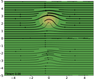
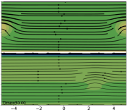
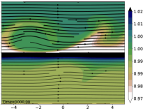
Figure 3: Snapshots of numerical solutions for two moving vortices at $t=\left\{0,50,1000\right\}$: two vortices propagate to the positive $x$-direction with a mean velocity of $0.05$ on $\Omega_{1}$ and $0.1$ on $\Omega_{2}$, respectively.

We integrate the coupled model by using RK4 (TC) with ${\triangle t}=0.025$ for $t\in\left[0,1000\right]$ over an ${N_{xe_{{}_{m}}}}(320)\times{N_{ye_{{}_{m}}}}(160)$ mesh. Figure 3 shows the snapshots of the density field at $t=\left\{0,50,1000\right\}$ with streamlines. Initially, two vortices are located at the center of each domain (left panel). Then they propagate to the positive $x$-direction with a different speed, so that the vortex on $\Omega_{2}$ moves two times faster than that on $\Omega_{1}$ (center panel). The velocity difference at the interface makes for the horizontal momentum to be transferred from the top (atmosphere) to the bottom (ocean) models. At the same time, since the bottom (ocean) is $10$\mathrm{\char 37\relax}$$ hotter than the top (atmosphere), heat transfer occurs from the bottom (ocean) to the top (atmosphere). Given the heat and horizontal momentum fluxes at the interface, we estimate the wall temperature and velocity for atmosphere and ocean models at the interface, respectively. The interface at the top (atmosphere) is warmed, but the bottom (ocean) counterpart is cooled. This situation leads to the sharp gradient of density at the interface. As time passes, the vortices get diffused because of viscosity and roll the fluids near the interface (right panel).

4.3.1 IMEX tight coupling methods

We now perform a temporal convergence study for IMEX coupling methods to demonstrate their stability (with $Cr>1$) and accuracy. Since both models have similar acoustic wave speed, it is difficult to relax the scale-separable stiffness with IMEX tight coupling methods. Instead, we add $z$-directional geometric stiffness to $\Omega_{1}$. The computational domain is discretized with $80\times 800$ on $\Omega_{1}$ and $80\times 80$ on $\Omega_{2}$. We treat $\Omega_{1}$ implicitly using the HEVI approach,, whereas we treat $\Omega_{2}$ explicitly so that the timestep size is restricted by the acoustic wave speed in $\Omega_{2}$.

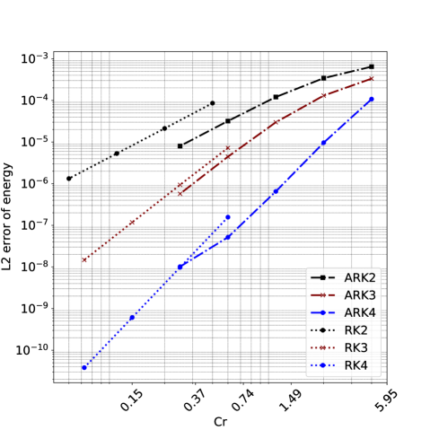
Figure 4: Two moving vortices: temporal convergence study for IMEX tight coupling methods. We take 1e-4 tolerance for the Krylov subspace solver.

We perform numerical simulations for IMEX tight coupling methods and measure the $L_{2}$ error at $t=2$ with the RK4 solution of ${\triangle t}=5\times 10^{-4}$. For comparison, we also conduct numerical simulations for RK tight coupling methods. The results are summarized in Table 3 and Figure 4. In general, the second-, third-, and fourth-order convergence rates are observed for both RK and ARK coupling methods in asymptotic regimes as expected. However, we observe that the rate of convergence of ARK4 decreases near $\mathcal{O}(10^{-8})$ error level. This decrease might be because we construct the linear operator $\mathbf{L}^{z}$ in (15) based on both analytical Jacobian and finite difference (FD) approximation in our implementation.

Table 3: Temporal convergence study conducted for RK and IMEX tight coupling methods. The domain is discretized with $80\times 800$ on $\Omega_{1}$ and $80\times 80$ on $\Omega_{2}$. We use the RK4 solution with ${\triangle t}=5\times 10^{-4}$ as the reference solution, and we measure the $L_{2}$ error at $t=2$. In general, the expected second-order, third-order, and fourth-order convergence rates are observed for both the RK and ARK ($\mathbf{L}^{z}$,TC) methods.

	$\triangle t(Cr_{1},Cr_{2})$	$\left\|\rho-\rho_{r}\right\|$		$\left\|\rho{\bf u}-\rho{\bf u}_{r}\right\|$		$\left\|\rho E-\rho E_{r}\right\|$
		error	order	error	order	error	order
RK2	0.004 (0.72,0.08)	3.128E-05	$-$	3.285E-05	$-$	8.606E-05	$-$
	0.002 (0.36,0.04)	7.730E-06	2.017	8.117E-06	2.017	2.126E-05	2.017
	0.001 (0.18,0.02)	1.929E-06	2.003	2.026E-06	2.003	5.306E-06	2.003
	0.0005(0.09,0.01)	4.821E-07	2.000	5.063E-07	2.000	1.326E-06	2.000
RK3	0.005 (0.89,0.10)	2.633E-06	$-$	2.765E-06	$-$	7.244E-06	$-$
	0.0025 (0.45,0.05)	3.413E-07	2.948	3.585E-07	2.948	9.390E-07	2.948
	0.00125 (0.22,0.02)	4.285E-08	2.994	4.500E-08	2.994	1.179E-07	2.994
	0.000625 (0.11,0.01)	5.358E-09	3.000	5.627E-09	3.000	1.474E-08	3.000
RK4	0.005 (0.89,0.10)	5.709E-08	$-$	5.996E-08	$-$	1.571E-07	$-$
	0.0025 (0.45,0.05)	3.558E-09	4.004	3.737E-09	4.004	9.789E-09	4.004
	0.00125 (0.22,0.02)	2.223E-10	4.000	2.333E-10	4.002	6.111E-10	4.002
	0.000625 (0.11,0.01)	1.420E-11	3.969	1.461E-11	3.997	3.817E-11	4.001
ARK2 ($\mathbf{L}^{z}$,TC)	0.04(7.15,0.76)	2.352E-04	$-$	2.447E-04	$-$	6.483E-04	$-$
	0.02(3.57,0.38)	1.248E-04	0.914	1.310E-04	0.901	3.433E-04	0.917
	0.01(1.79,0.19)	4.395E-05	1.506	4.616E-05	1.505	1.209E-04	1.506
	0.005(0.89,0.10)	1.163E-05	1.919	1.221E-05	1.919	3.198E-05	1.919
	0.0025(0.45,0.05)	2.919E-06	1.994	3.065E-06	1.994	8.030E-06	1.994
ARK3 ($\mathbf{L}^{z}$,TC)	0.04(7.15,0.76)	1.214E-04	$-$	1.275E-04	$-$	3.341E-04	$-$
	0.02(3.57,0.38)	4.758E-05	1.352	4.997E-05	1.352	1.309E-04	1.352
	0.01(1.79,0.19)	1.086E-05	2.132	1.140E-05	2.132	2.987E-05	2.132
	0.005(0.89,0.10)	1.621E-06	2.744	1.702E-06	2.744	4.459E-06	2.744
	0.0025(0.45,0.05)	2.082E-07	2.960	2.187E-07	2.960	5.729E-07	2.960
ARK4 ($\mathbf{L}^{z}$,TC)	0.04(7.15,0.76)	3.911E-05	$-$	4.108E-05	$-$	1.076E-04	$-$
	0.02(3.57,0.38)	3.515E-06	3.476	3.692E-06	3.476	9.670E-06	3.476
	0.01(1.79,0.19)	2.371E-07	3.890	2.507E-07	3.881	6.521E-07	3.890
	0.005(0.89,0.10)	1.888E-08	3.650	2.162E-08	3.535	5.166E-08	3.658
	0.0025(0.45,0.05)	3.782E-09	2.320	5.073E-09	2.092	1.018E-08	2.343

4.3.2 IMEX loose coupling (concurrent and sequential coupling) methods

The IMEX tight coupling approach can achieve high-order convergence in time, but it requires communication at each stage. Moreover, both the models advance with the same timestep size. We may relax the tight coupling condition by using concurrent and sequential couplings, as shown in Figure 2(b) and Figure 2(c). In IMEX loose coupling methods, we solve the bottom (ocean) model implicitly using ARK time integrators but treat the top (atmosphere) model explicitly using the explicit part of ARK methods. The computational domain is discretized with $80\times 400$ elements on $\Omega_{1}$ and $80\times 160$ elements on $\Omega_{2}$.

We measure the $L_{2}$ error at $t=2$ with the reference RK4 solution of ${\triangle t}=5\times 10^{-4}$ and report the results in Table 4. Since the top (atmosphere) model has two substeps, the Courant number at each substep should be understood as $\frac{1}{2}Cr_{2}$ in Table 4. Unlike IMEX tight coupling methods, both the concurrent (CC2) and the sequential (SC2) coupling methods show first-order convergence rates for density, momentum, and total energy. The difference between two error levels of CC2 and SC2 is within $\mathcal{O}(10^{-5})$.

Table 4: Temporal convergence study conducted for IMEX loose coupling methods. The domain is discretized with $80\times 400$ on $\Omega_{1}$ and $80\times 160$ on $\Omega_{2}$. We use the RK4 solution with ${\triangle t}=5\times 10^{-4}$ as the reference solution, and we measure the $L_{2}$ error at $t=2$.

	$\triangle t(Cr_{1},Cr_{2})$	$\left\|\rho-\rho_{r}\right\|$		$\left\|\rho{\bf u}-\rho{\bf u}_{r}\right\|$		$\left\|\rho E-\rho E_{r}\right\|$
		error	order	error	order	error	order
ARK2 ($\mathbf{L}^{z}$,CC2)	0.05 (4.47,1.91)	3.849E-04	$-$	3.969E-04	$-$	1.033E-03	$-$
	0.025 (2.23,0.95)	1.781E-04	1.112	1.832E-04	1.115	4.764E-04	1.117
	0.0125 (1.12,0.48)	5.539E-05	1.685	5.513E-05	1.733	1.413E-04	1.753
	0.00625 (0.56,0.24)	1.696E-05	1.707	1.522E-05	1.857	3.702E-05	1.933
	0.003125(0.28,0.12)	6.371E-06	1.413	4.839E-06	1.653	1.030E-05	1.846
	0.001563(0.14,0.06)	2.865E-06	1.153	1.929E-06	1.327	3.446E-06	1.579
	0.000781(0.07,0.03)	1.390E-06	1.043	8.944E-07	1.109	1.441E-06	1.258
ARK2 ($\mathbf{L}^{z}$,SC2)	0.05 (4.47,1.91)	3.835E-04	$-$	3.954E-04	$-$	1.032E-03	$-$
	0.025 (2.23,0.95)	1.773E-04	1.113	1.823E-04	1.117	4.754E-04	1.118
	0.0125 (1.12,0.48)	5.468E-05	1.697	5.430E-05	1.747	1.403E-04	1.760
	0.00625 (0.56,0.24)	1.636E-05	1.741	1.443E-05	1.911	3.597E-05	1.964
	0.003125(0.28,0.12)	5.962E-06	1.456	4.187E-06	1.785	9.289E-06	1.953
	0.001563(0.14,0.06)	2.635E-06	1.178	1.498E-06	1.483	2.624E-06	1.824
	0.000781(0.07,0.03)	1.272E-06	1.051	6.556E-07	1.192	9.070E-07	1.532
ARK3 ($\mathbf{L}^{z}$,CC2)	0.05 (4.47,1.91)	2.074E-04	$-$	2.040E-04	$-$	5.208E-04	$-$
	0.025 (2.23,0.95)	7.514E-05	1.464	6.949E-05	1.554	1.720E-04	1.598
	0.0125 (1.12,0.48)	2.467E-05	1.607	1.807E-05	1.943	3.688E-05	2.222
	0.00625 (0.56,0.24)	1.112E-05	1.150	7.116E-06	1.344	1.133E-05	1.703
	0.003125(0.28,0.12)	5.513E-06	1.012	3.490E-06	1.028	5.375E-06	1.075
ARK3 ($\mathbf{L}^{z}$,SC2)	0.05 (4.47,1.91)	2.068E-04	$-$	2.008E-04	$-$	5.161E-04	$-$
	0.025 (2.23,0.95)	7.494E-05	1.465	6.708E-05	1.582	1.682E-04	1.617
	0.0125 (1.12,0.48)	2.458E-05	1.608	1.565E-05	2.099	3.219E-05	2.386
	0.00625 (0.56,0.24)	1.109E-05	1.148	5.521E-06	1.504	6.927E-06	2.216
	0.003125(0.28,0.12)	5.506E-06	1.010	2.677E-06	1.044	2.986E-06	1.214
ARK4 ($\mathbf{L}^{z}$,CC2)	0.05 (4.47,1.91)	9.853E-05	$-$	7.092E-05	$-$	1.417E-04	$-$
	0.025 (2.23,0.95)	4.462E-05	1.143	2.839E-05	1.321	4.447E-05	1.671
	0.0125 (1.12,0.48)	2.215E-05	1.011	1.403E-05	1.016	2.170E-05	1.035
	0.00625 (0.56,0.24)	1.105E-05	1.004	6.997E-06	1.004	1.080E-05	1.006
	0.003125(0.28,0.12)	5.515E-06	1.002	3.493E-06	1.002	5.390E-06	1.003
ARK4 ($\mathbf{L}^{z}$,SC2)	0.05 (4.47,1.91)	9.884E-05	$-$	6.078E-05	$-$	1.207E-04	$-$
	0.025 (2.23,0.95)	4.505E-05	1.134	2.204E-05	1.463	2.565E-05	2.234
	0.0125 (1.12,0.48)	2.243E-05	1.006	1.089E-05	1.016	1.217E-05	1.076
	0.00625 (0.56,0.24)	1.120E-05	1.002	5.441E-06	1.002	6.069E-06	1.004
	0.003125(0.28,0.12)	5.598E-06	1.001	2.719E-06	1.001	3.030E-06	1.002

4.4 CNS2: Wind-driven flow

The ocean current is driven by the wind at the sea surface. Under the assumption of the rigid-lid interface, we mimic the wind-driven flows for a coupled compressible Navier–Stokes equation. The computational domain is the same as the one in Section 4.3. We take $T_{\infty_{1}}=1.1$, $T_{\infty_{2}}=1$, and $\rho_{\infty_{1}}=\rho_{\infty_{2}}=1$ with $Pr=0.72$ and $\gamma=1.4$. We impose a horizontally moving isothermal wall condition at the top boundary, for example, $T_{w_{2}}=0.9$ and $u_{w_{2}}=0.1$, and an isothermal no-slip condition at the bottom wall, for example, $T_{w_{1}}=1$ and $u_{w_{1}}=0$. We apply periodic boundary conditions laterally on $\Omega_{2}$ and adiabatic no-slip wall boundary conditions at the left and the right walls on $\Omega_{1}$. We set uniform horizontal flows $u_{\infty_{2}}=0.1$ on $\Omega_{2}$ and zero velocity on $\Omega_{1}$. Similar to the lid-driven cavity flow [63], the viscous drag force exerted by the velocity difference at the interface induces circular motion on $\Omega_{1}$.

We perform simulations for $\tilde{\mu}_{m}=\left\{10^{-1},500^{-1},1000^{-1},5000^{-1}\right\}$ on the grid with $80\times 80$ elements on $\Omega_{1}$ and $80\times 80$ elements on $\Omega_{2}$ using RK4 methods. In Figure 5, temperature fields for $\tilde{\mu}_{m}=\left\{10^{-1},500^{-1},1000^{-1},5000^{-1}\right\}$ are contoured with streamlines at $t=500$. Since the heat and momentum fluxes are proportional to $\tilde{\mu}_{m}$, as shown for $\tilde{\mu}_{m}=100^{-1}$, the temperature $T_{1}=1.1$ quickly cools to $T_{1}=1.0$, compared with other cases (for $\tilde{\mu}_{m}=\left\{500^{-1},1000^{-1},5000^{-1}\right\}$). As a result, the horizontal momentum becomes the main driving source for the flows on $\Omega_{1}$. As we decrease $\tilde{\mu}_{m}$, the heat transfer becomes weaker. Thus, sharp gradients of temperature fields are observed near the interface and the boundaries at the top and the bottom. The temperature gradients induce the vertical motion of the fluid $\Omega_{1}$, which pushes the center of the circulation toward the right wall, as shown for $\tilde{\mu}_{m}=5000^{-1}$.

Since this case clearly shows how cooled fluid moves away from the interface, we choose it for the comparison of IMEX coupling methods in the following section.

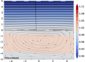
(a) $\tilde{\mu}_{m}=100^{-1}$

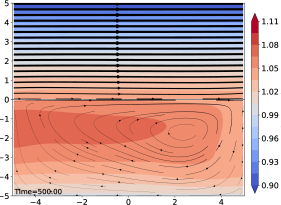
(b) $\tilde{\mu}_{m}=500^{-1}$

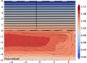
(c) $\tilde{\mu}_{m}=1000^{-1}$

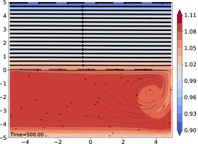
(d) $\tilde{\mu}_{m}=5000^{-1}$

Figure 5: Wind-driven flows: the snapshots of the temperature field at $t=500$. Simulations are performed on the grid with $80\times 80$ elements on $\Omega_{1}$ and $80\times 80$ elements on $\Omega_{2}$ using RK4 methods.

4.4.1 IMEX coupling methods for $\tilde{\mu}_{m}=5000^{-1}$

We first conduct numerical experiments for ARK4($\mathbf{L}^{z}$,TC) on the grid with $100\times 500$ elements on $\Omega_{1}$ and $100\times 80$ elements on $\Omega_{2}$ for $t\in\left\{0,500\right\}$. The timestep size is taken as ${\triangle t}=0.05$, which corresponds to $Cr_{1}=5.38$ and $Cr_{2}=0.88$. In Figure 6 we plot the temperature fields with streamlines (black solid lines) over the simulation period. We see the temperature near the top and the bottom boundaries decreases because of the cold wall boundary condition. At the interface, the temperature is getting hotter on $\Omega_{2}$ and colder on $\Omega_{1}$ through the heat exchange. The cooled fluid moves along the right wall and rolls up following the circulation at $t=500$. The temperature field as well as the streamline at $t=500$ shows good agreement with the RK4 solution in Figure 7(a). The difference between RK4 and ARK4 ($\mathbf{L}^{z}$,TC) is within $\mathcal{O}(10^{-5})$ in Figure 7(b).

Now we compare the performance of IMEX coupling methods. We choose the largest timestep size for each IMEX coupling method. We take the RK4 (with ${\triangle t}=0.01$) solution as a reference and measure the $L_{2}$ relative errors. In Table 5 we summarize the relative errors and wall-clock times for IMEX coupling methods. The relative errors of TC, SC2, and CC2 coupling methods for ARK3 have the same order of accuracy for density, momentum, and total energy. For example, the order of relative error for density is $\mathcal{O}(10^{-4})$. Similarly, the relative errors of ARK2 ($\mathbf{L}^{z}$, SC2) and ARK2 ($\mathbf{L}^{z}$, CC2) have $\mathcal{O}(10^{-4})$ order of accuracy for density, momentum, and total energy. Compared with ARK3 ($\mathbf{L}^{z}$, TC), ARK4 ($\mathbf{L}^{z}$, TC) is closer to the RK4 solution. However, ARK2 ($\mathbf{L}^{z}$, SC2/CC2) has a smaller relative error compared with that of ARK3 ($\mathbf{L}^{z}$, SC2/CC2). Compared to ARK4 ($\mathbf{L}^{z}$, SC2/CC2), ARK2 ($\mathbf{L}^{z}$, SC2/CC2) has slightly smaller relative errors of density and total energy. From an accuracy point of view, IMEX tight coupling benefits from using high-order methods; however, IMEX loose coupling does not. The reason may be that the heat and the horizontal momentum fluxes are not continuous at the interface for IMEX loose coupling schemes. From a stability viewpoint, ARK2 ($\mathbf{L}^{z}$, SC2/CC2) is more stable than ARK2 ($\mathbf{L}^{z}$, TC). This is because the Courant number at each substep for ARK2 ($\mathbf{L}^{z}$, SC2/CC2) becomes smaller than ARK2 ($\mathbf{L}^{z}$, TC) counterpart. By increasing subcycles in the explicit part. the acoustic mode in atmospheric model is resolved with smaller timestep size. As for the computational cost, IMEX ARK2 and ARK3 coupling schemes are comparable to the RK4 tight coupling method.

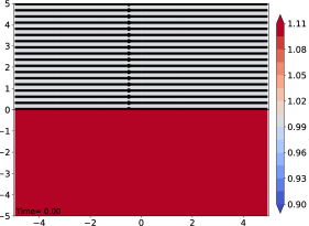
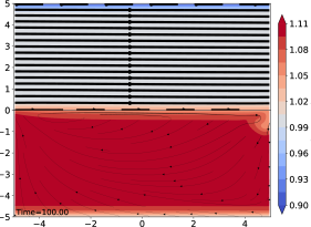
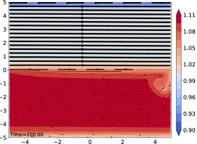
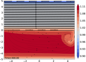
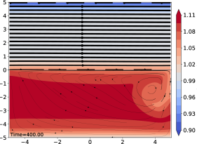
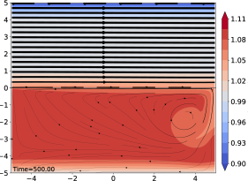
Figure 6: Evolution of the temperature field for the wind-driven flows: simulation is conducted with the ARK4 ($\mathbf{L}^{z}$,TC) method over a mesh of $100\times 500$ elements on $\Omega_{1}$ and $100\times 80$ elements on $\Omega_{2}$ for $t\in\left[0,500\right]$. Black solid lines represent streamline, and the color bar shows the range of temperature from $0.9$ to $1.1$.

Table 5: Relative errors and wall-clock times for IMEX coupling methods with respect to the RK4 (${\triangle t}=0.01$) coupling at $t=500$. The domain is discretized with $100\times 500$ on $\Omega_{1}$ and $100\times 80$ on $\Omega_{2}$. $Cr_{2}$ is the Courant number for the entire timestep; the substep number needs to be scaled by 1/2 for SC2 and CC2.

	$\triangle t(Cr_{1},Cr_{2})$	$\left\|\rho-\rho_{r}\right\|$	$\left\|\rho{\bf u}-\rho{\bf u}_{r}\right\|$	$\left\|\rho E-\rho E_{r}\right\|$	wc[s]
RK4	0.01 (1.08,0.18)	-	-	-	5570.06
ARK2 ($\mathbf{L}^{z}$,TC)	0.04 (4.20,0.70)	7.435E-05	2.049E-04	1.989E-04	3322.84
ARK2 ($\mathbf{L}^{z}$,SC2)	0.05 (5.24,0.88)	1.310E-04	3.075E-04	3.318E-04	3280.01
ARK2 ($\mathbf{L}^{z}$,CC2)	0.05 (5.24,0.88)	1.393E-04	3.082E-04	3.323E-04	3312.13
ARK3 ($\mathbf{L}^{z}$,TC)	0.05 (5.24,0.88)	7.231E-04	1.128E-03	1.959E-03	5214.52
ARK3 ($\mathbf{L}^{z}$,SC2)	0.05 (5.24,0.88)	7.266E-04	1.128E-03	1.959E-03	5400.41
ARK3 ($\mathbf{L}^{z}$,CC2)	0.05 (5.24,0.88)	7.336E-04	1.129E-03	1.959E-03	5363.56
ARK4 ($\mathbf{L}^{z}$,TC)	0.05 (5.24,0.88)	1.468E-04	1.661E-04	3.956E-04	6355.54
ARK4 ($\mathbf{L}^{z}$,SC2)	0.05 (5.24,0.88)	1.452E-04	1.641E-04	3.961E-04	7361.94
ARK4 ($\mathbf{L}^{z}$,CC2)	0.05 (5.24,0.88)	1.452E-04	1.660E-04	3.966E-04	7867.85

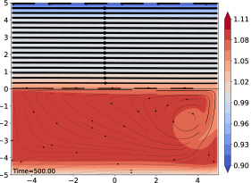
(a) RK4

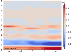
(b) Difference

Figure 7: Wind-driven flows at $t=500$: (a) temperature field with streamlines of the RK4 solution and (b) the difference between ARK4 ($\mathbf{L}^{z}$,TC) and RK4. Simulations are performed on the grid with $100\times 500$ elements on $\Omega_{1}$ and $100\times 80$ elements on $\Omega_{2}$. We take ${\triangle t}=0.05$ for ARK4 ($\mathbf{L}^{z}$,TC) and ${\triangle t}=0.01$ for RK4.

4.5 CNS2: Wind-driven flows with Kelvin–Helmholtz instability

Kelvin–Helmholtz instability (KHI) is an important mechanism in the development of turbulence in the stratified atmosphere and ocean. KHI arises when two fluids have different densities and tangential velocities across the interface. Small disturbances such as waves at the interface grow exponentially, and the interface rolls up into KH rotors [64, 65, 66]. To see the nonlinear evolution of KHI, we add a jet to $\Omega_{2}$ in the wind-driven example above. We also place a vortex on $\Omega_{1}$. Boundary conditions are the same as in the wind-driven example. The initial conditions are chosen as

$$\rho_{1} =\left(1-\frac{(\gamma-1)\beta^{2}}{8\alpha\gamma\pi^{2}}e^{\alpha\left(1-r^{2}\right)}\right)^{\frac{1}{\gamma-1}},$$

$$u_{1} =\frac{\beta}{2\pi}\tilde{z}_{1}e^{\frac{\alpha}{2}\left(1-r^{2}\right)},$$

$$w_{1} =-\frac{\beta}{2\pi}\tilde{x}_{1}e^{\frac{\alpha}{2}\left(1-r^{2}\right)},$$

$${{p}}_{1} =1.1\gamma^{-1}\rho_{1}^{\gamma}$$

with $r=\|{\bf x}-\tilde{{\bf x}}\|$, $\tilde{x}_{1}=x_{1}-x_{c}$, $\tilde{z}_{1}=z_{1}-z_{c}$ for $\Omega_{1}$,

$$\rho_{2} =1+\frac{1}{2}\left(\tanh\left(\frac{z_{2}-s_{1}}{a}\right)-\tanh\left(\frac{z_{2}-s_{2}}{a}\right)\right),$$

$$u_{2} =0.1+\left(\tanh\left(\frac{z_{2}-s_{1}}{a}\right)-\tanh\left(\frac{z_{2}-s_{2}}{a}\right)-1\right),$$

$$w_{2} =A\sin\left(2\pi x_{2}\right)\left(\exp\left(-\frac{(z_{2}-s_{1})^{2}}{\sigma^{2}}\right)+\exp\left(-\frac{(z_{2}-s_{2})^{2}}{\sigma^{2}}\right)\right),$$

$${{p}}_{2} =\gamma^{-1}$$

for $\Omega_{2}$. Here, we take $a=0.05$, $A=0.01$, $\sigma=0.2$, $s_{1}=2$, $s_{2}=3$, ${\bf x}_{c}=(0,-3)$, $\alpha=5$ and $\beta=0.5$. We choose the fluid parameters of $\gamma=1.4$, $Pr=0.72$, $\tilde{c}_{p}=(\gamma-1)^{-1}$, and $\tilde{\mu}_{m}=5000^{-1}$.

We conduct the simulation with the ARK4 ($\mathbf{L}^{z}$,TC) method over the mesh of $100\times 400$ elements on $\Omega_{1}$ and $100\times 80$ elements on $\Omega_{2}$ in Figure 8. The evolution of temperature fields is shown for $t\in\left[0,500\right]$. Kelvin–Helmholtz waves are well developed at $t=100$ and start to diffuse while mixing fluids. Meanwhile, because of the heat and horizontal momentum exchange, fluid on $\Omega_{1}$ cools near the interface and moves along the outside of vortex as time passes.

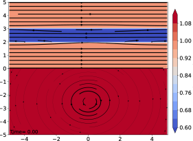
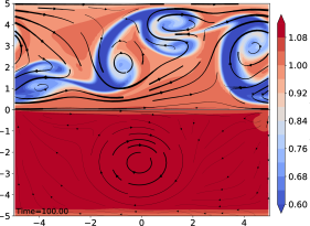
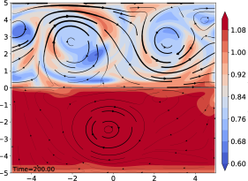
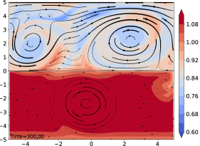
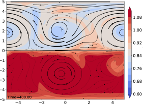
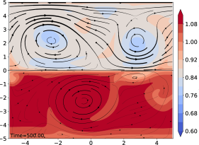
Figure 8: Evolution of the temperature field for the wind-driven flows with Kelvin–Helmholtz instability: simulation is conducted with the ARK4 ($\mathbf{L}^{z}$,TC) method over a mesh of $100\times 400$ elements on $\Omega_{1}$ and $100\times 80$ elements on $\Omega_{2}$ for $t\in\left[0,500\right]$.

Figure 9 shows temperature fields at $t=500$ for RK4, ARK2 ($\mathbf{L}^{z}$,TC), ARK2 ($\mathbf{L}^{z}$,SC2), and ARK2 ($\mathbf{L}^{z}$,CC2). We choose the timestep sizes as ${\triangle t}=0.01$ for RK4, ${\triangle t}=0.04$ for ARK2 ($\mathbf{L}^{z}$,TC), ${\triangle t}=0.05$ for ARK2 ($\mathbf{L}^{z}$,SC2) and ARK2 ($\mathbf{L}^{z}$,CC2), and ${\triangle t}=0.1$ for ARK2 ($\mathbf{L}$,SC8) and ARK2 ($\mathbf{L}$,CC8). In general, all ARK2 solutions demonstrate good agreement with the RK4 solution.

(a) RK4

(b) ARK2($\mathbf{L}^{z}$,TC)

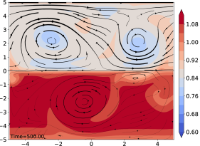
(c) ARK2($\mathbf{L}^{z}$,SC2)

(d) ARK2($\mathbf{L}^{z}$,CC2)

(e) ARK2($\mathbf{L}$,SC8)

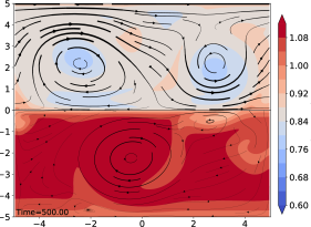
(f) ARK2($\mathbf{L}$,CC8)

Figure 9: Temperature fields for KHI at $t=500$: (a) RK4, (b) ARK2($\mathbf{L}^{z}$,TC), (c) ARK2($\mathbf{L}^{z}$,SC2), (d) ARK2($\mathbf{L}^{z}$,CC2), (e) ARK2($\mathbf{L}$,SC8), and (f) ARK2($\mathbf{L}$,CC8) coupling methods. Simulations are performed on a grid with $100\times 400$ elements on $\Omega_{1}$ and $100\times 80$ elements on $\Omega_{2}$.

In Table 6 we report the relative errors of several IMEX coupling methods with respect to the RK4 solution (with ${\triangle t}=0.01$). Compared with concurrent coupling (CC) methods, sequential coupling (SC) methods show slightly better accuracy. The relative errors of ARK2 ($\mathbf{L}^{z}$,SC2) and ARK3 ($\mathbf{L}^{z}$,SC2) are smaller than those of the ARK2 ($\mathbf{L}^{z}$,CC2) and ARK3 ($\mathbf{L}^{z}$,CC2) within $\mathcal{O}(10^{-4})$. Similarly, ARK2 ($\mathbf{L}^{z}$,SC8) has small relative errors of density, momentum, and total energy compared with those of ARK2 ($\mathbf{L}^{z}$,CC8). With the same timestep size, the ARK4 ($\mathbf{L}^{z}$,TC) solution is closer to the RK4 solution than that of ARK3 ($\mathbf{L}^{z}$,TC). With loose coupling (SC2 and CC2) methods, ARK4 ($\mathbf{L}^{z}$, SC2/CC2) shows better accuracy than ARK2 ($\mathbf{L}^{z}$, SC2/CC2) for density and total energy, and ARK3 ($\mathbf{L}^{z}$, SC2/CC2) for all variables. However, the ARK3 ($\mathbf{L}^{z}$) solutions are farther away from the RK4 solution than that of ARK2 ($\mathbf{L}^{z}$). Nevertheless, with the same timestep, the loose coupling (SC2 and CC2) methods produce closer solutions to RK4 than do the tight coupling methods because SC2 and CC2 have two explicit subcycles. We have already observed similar behavior in the wind-driven flow example. When we double the timestep size of ARK2 ($\mathbf{L}^{z}$,SC2/CC2), the solutions become unstable. The linear operator $\mathbf{L}^{z}$ is not sufficient to capture the stiff components in the system when ${\triangle t}=0.1$. However, ARK2 ($\mathbf{L}$,SC8/CC8) with ${\triangle t}=0.1$ results in stable solutions. This result implies that as we increase a timestep size beyond a certain Courant number (between $Cr_{1}=4.56$ and $Cr_{1}=9.13$), the viscous part becomes stiff and thus starts to affect the numerical stability. Including the viscous part to the linear operator enhances numerical stability but also increase computational cost in this study. As for wall-clock time, ARK2 ($\mathbf{L}^{z}$) is cheaper than RK4, and ARK3 ($\mathbf{L}^{z}$) is comparable to RK4 in this example. Note that we introduce geometric stiffness vertically to use the HEVI approach. When a mesh is anisotropic, IMEX coupling methods can be beneficial.

Table 6: Relative errors and wall-clock times for IMEX coupling methods with respect to the RK4 coupling at $t=500$. The domain is discretized with $100\times 400$ on $\Omega_{1}$ and $100\times 80$ on $\Omega_{2}$. $Cr_{2}$ is the Courant number for the entire timestep; the substep number needs to be scaled by $1/k$ for SC$\{k\}$ and CC$\{k\}$.

	$\triangle t(Cr_{1},Cr_{2})$	$\left\|\rho-\rho_{r}\right\|$	$\left\|\rho{\bf u}-\rho{\bf u}_{r}\right\|$	$\left\|\rho E-\rho E_{r}\right\|$	wc[s]
RK4	0.01 (0.91,0.18)	-	-	-	3968.209
ARK2 ($\mathbf{L}^{z}$,TC)	0.04(3.65,0.70)	5.768E-03	3.534E-03	7.369E-04	2407.544
ARK2 ($\mathbf{L}^{z}$,SC2)	0.05(4.56,0.88)	1.143E-03	5.181E-04	6.271E-04	2356.430
ARK2 ($\mathbf{L}^{z}$,CC2)	0.05(4.56,0.88)	1.757E-03	8.697E-04	6.612E-04	2240.349
ARK2 ($\mathbf{L}^{z}$,SC8)	0.05(4.56,0.88)	8.361E-04	6.511E-04	6.220E-04	2929.486
ARK2 ($\mathbf{L}^{z}$,CC8)	0.05(4.56,0.88)	1.437E-03	9.995E-04	6.597E-04	2999.596
ARK2 ($\mathbf{L}$,SC8)	0.10(9.13,1.76)	1.631E-03	1.305E-03	1.569E-03	6794.486
ARK2 ($\mathbf{L}$,CC8)	0.10(9.13,1.76)	2.916E-03	1.987E-03	1.633E-03	6542.753
ARK3 ($\mathbf{L}^{z}$,TC)	0.05(4.56,0.88)	1.160E-02	7.594E-03	2.373E-03	3403.247
ARK3 ($\mathbf{L}^{z}$,SC2)	0.05(4.56,0.88)	1.171E-03	1.284E-03	2.170E-03	3781.536
ARK3 ($\mathbf{L}^{z}$,CC2)	0.05(4.56,0.88)	1.719E-03	1.605E-03	2.184E-03	3890.584
ARK4 ($\mathbf{L}^{z}$,TC)	0.05(4.56,0.88)	4.452E-03	2.702E-03	4.910E-04	4706.067
ARK4 ($\mathbf{L}^{z}$,SC2)	0.05(4.56,0.88)	9.121E-04	7.120E-04	3.522E-04	5402.731
ARK4 ($\mathbf{L}^{z}$,CC2)	0.05(4.56,0.88)	1.475E-03	1.084E-03	4.261E-04	5120.688

Next we plot the time series of total mass and total energy losses in Figure 10. The total mass and total energy losses are defined by

mass loss $$:=\left|\text{mass}(t)-\text{mass}(0)\right|,$$

energy loss $$:=\left|\text{energy}(t)-\text{energy}(0)\right|,$$

where

$$\text{energy}=\int_{\Omega_{1}}\rho Ed\Omega_{1}+\int_{\Omega_{2}}\rho Ed\Omega_{2}=\sum_{m=1}^{2}\sum_{\ell=1}^{{N_{E_{m}}}}\overline{\rho E}_{m_{\ell}}\left|K_{m_{\ell}}\right|$$

and $\overline{\rho E}_{m_{\ell}}=\left|K_{m_{\ell}}\right|^{-1}\int_{K_{m_{\ell}}}\rho EdK$. In Figure 10(a) we numerically observe that total mass is conserved with IMEX coupling methods regardless of tight or loose coupling methods. The total mass losses for IMEX tight and loose coupling methods are within $\mathcal{O}(10^{-13})$. This means that the total mass changes with time, but fluates around the initial total mass within $10^{-13}$. This result makes sense because we do not exchange the mass across the interface but adjust the wall temperature in the interface. This rigid-lid condition blocks the vertical motion of the interface: no mass flux is allowed, and hence the total mass is conserved. As for the total energy loss, a peak is observed near $t=100$ (when strong KHI is observed in Figure 8), and then the total energy loss decreases as time passes.

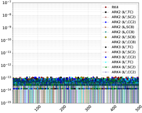
(a) Mass loss

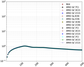
(b) Total energy loss

Figure 10: Wind-driven flows with KHI: histories of (a) total mass loss and (b) total energy loss for $t\in\left[0,500\right]$. Total mass loss is bounded within $\mathcal{O}(10^{-13})$. Total energy loss has a peak near $t=100$ when strong KHI is observed in Figure 8.

5 Conclusions

In this paper, we have developed IMEX coupling methods for compressible Navier–Stokes systems with the rigid-lid coupling condition arising from the atmosphere and the ocean interaction. We compute horizontal momentum and heat fluxes across the interface by using the bulk formula, from which we estimate wall temperature and horizontal velocity. These estimated values serve as the isothermal moving wall boundary conditions on each model. Each model is solved within the IMEX (tight or loose) coupling framework. IMEX coupling methods solve one domain (atmosphere) explicitly and the other (ocean) implicitly. To enhance computation efficiency, we adapt IMEX time integrators, which can handle scale-separable stiffness or geometrically induced stiffness, as an implicit solver for the ocean model. Furthermore, we employ a horizontally explicit and vertically implicit (HEVI) approach where solutions are obtained column by column; hence, the resulting linear system is significantly reduced compared with two-dimensional IMEX methods.

IMEX tight coupling methods naturally support two-way coupling at every stage. Thus, the continuity of the heat and the horizontal momentum fluxes is guaranteed by construction. These methods also facilitate high-order solutions in time and relax geometrically induced stiffness. However, IMEX tight coupling methods treat one domain (atmosphere) explicitly, and therefore the stiffness in the domain (atmosphere) restricts the maximum timestep size. Also, each coupled model advances with the same timestep size. We can alleviate the restriction by loosening the tight coupling condition. That is, instead of two-way coupling at each stage, we exchange the interface information at a certain time. Heat and horizontal momentum fluxes are no longer continuous across the interface at the stages, but total mass is strictly conserved. In the Kelvin–Helmholtz instability example, the total mass loss is less than $\mathcal{O}(10^{-13})$. We conjecture that the total mass will still be conserved with other formulations such as a coupled compressible and incompressible Navier–Stokes systems as long as the spatial discretization is conservative. As for temporal convergence, IMEX loose coupling methods achieve a first-order convergent rate in the two moving-vortex example. However, the relative errors of the IMEX loose coupling schemes are smaller than those of their IMEX tight coupling counterparts. The reason is that the temporal discretization errors are reduced by adding substeps.

We have investigated two loose coupling strategies: concurrent and sequential. Both exchange interface solutions before advancing the ocean model. In concurrent coupling, each model is run independently, which is attractive for parallel computing. In contrast, in sequential coupling, the ocean model is run first and then the atmospheric model is advanced with a number of substeps. In the latter case, because all stage values from the ocean model are available, necessary interface information can be interpolated and transferred from the ocean model to the atmospheric model at each stage. This capability slightly improves the accuracy but is not significant in our simulations.

We also observe that the choice of the linear operator affects numerical stability. The viscous term is not a dominant source of stiffness with a small timestep size; thus the linear operator $\mathbf{L}^{z}$ is sufficient to relax stiffness in the ocean model. As the timestep size increases, however, $\mathbf{L}^{z}$ is not sufficient because viscous terms become stiffer. In this case, using the linear $\mathbf{L}$ that contains both the inviscid and the viscous parts increases coupling stability. As for the computational cost, the ARK2 ($\mathbf{L}^{z}$) and ARK3 ($\mathbf{L}^{z}$) coupling methods show wall-clock time comparable to that of the RK4 method within $\mathcal{O}(10^{-2})$ relative errors. Note that for compressible Navier–Stokes systems, the relative errors of IMEX coupling methods are caused mainly by suppressing fast acoustic waves. The flow patterns of IMEX couplings methods show good agreement with the RK counterpart in our numerical examples.

In the current study, we investigated IMEX coupling schemes on two ideal gas fluids without gravity. For realistic atmosphere and ocean interaction, the gravity source term and the material properties of the ocean should be taken into account. Also, coupling incompressible and compressible Navier–Stokes system is also worthwhile for reflecting the current global atmosphere and ocean models. Since these may affect the stability of coupling schemes, ongoing work focuses on improving our testbed to fit realistic models in modern computing architectures. Other time integrators such as multirate or exponential integrators may represent more effective ways for addressing limitations in the couple performance.

Government License (will be removed at publication): The submitted manuscript has been created by UChicago Argonne, LLC, Operator of Argonne National Laboratory (“Argonne”). Argonne, a U.S. Department of Energy Office of Science laboratory, is operated under Contract No. DE-AC02-06CH11357. The U.S. Government retains for itself, and others acting on its behalf, a paid-up nonexclusive, irrevocable worldwide license in said article to reproduce, prepare derivative works, distribute copies to the public, and perform publicly and display publicly, by or on behalf of the Government. The Department of Energy will provide public access to these results of federally sponsored research in accordance with the DOE Public Access Plan. http://energy.gov/downloads/doe-public-access-plan.

References

- [1] J.-C. Golaz, P. M. Caldwell, L. P. Van Roekel, M. R. Petersen, Q. Tang, J. D. Wolfe, G. Abeshu, V. Anantharaj, X. S. Asay-Davis, D. C. Bader, et al., The DOE E3SM coupled model version 1: Overview and evaluation at standard resolution, Journal of Advances in Modeling Earth Systems 11 (7) (2019) 2089–2129.
- [2] W. Hazeleger, C. Severijns, T. Semmler, S. cStefuanescu, S. Yang, X. Wang, K. Wyser, E. Dutra, J. M. Baldasano, R. Bintanja, et al., EC-Earth: a seamless earth-system prediction approach in action, Bulletin of the American Meteorological Society 91 (10) (2010) 1357–1364.
- [3] P. Gentine, J. K. Green, M. Guérin, V. Humphrey, S. I. Seneviratne, Y. Zhang, S. Zhou, Coupling between the terrestrial carbon and water cycles a review, Environmental Research Letters 14 (8) (2019) 083003.
- [4] S. Burrows, M. Maltrud, X. Yang, Q. Zhu, N. Jeffery, X. Shi, D. Ricciuto, S. Wang, G. Bisht, J. Tang, et al., The DOE E3SM v1. 1 biogeochemistry configuration: description and simulated ecosystem-climate responses to historical changes in forcing, Journal of Advances in Modeling Earth Systems 12 (9) (2020) e2019MS001766.
- [5] W. D. Collins, C. M. Bitz, M. L. Blackmon, G. B. Bonan, C. S. Bretherton, J. A. Carton, P. Chang, S. C. Doney, J. J. Hack, T. B. Henderson, et al., The Community Climate System Model version 3 (CCSM3), Journal of Climate 19 (11) (2006) 2122–2143.
- [6] T. R. Anderson, E. Hawkins, P. D. Jones, CO2, the greenhouse effect and global warming: from the pioneering work of arrhenius and callendar to today’s Earth System Models, Endeavour 40 (3) (2016) 178–187.
- [7] M. J. Hoffman, X. Asay-Davis, S. F. Price, J. Fyke, M. Perego, Effect of subshelf melt variability on sea level rise contribution from thwaites glacier, antarctica, Journal of Geophysical Research: Earth Surface.
- [8] A. P. Craig, M. Vertenstein, R. Jacob, A new flexible coupler for earth system modeling developed for CCSM4 and CESM1, The International Journal of High Performance Computing Applications 26 (1) (2012) 31–42.
- [9] R. Jacob, J. Larson, E. Ong, MN communication and parallel interpolation in Community Climate System Model version 3 using the Model Coupling Toolkit, The International Journal of High Performance Computing Applications 19 (3) (2005) 293–307.
- [10] S. Valcke, The OASIS3 coupler: A European climate modelling community software, Geoscientific Model Development 6 (2) (2013) 373.
- [11] R. Hallberg, Numerical instabilities of the ice/ocean coupled system, in: CLIVAR WGOMD Workshop on high, 2014, p. 38.
- [12] F. Lemarié, E. Blayo, L. Debreu, Analysis of ocean-atmosphere coupling algorithms: consistency and stability, Procedia Computer Science 51 (2015) 2066–2075.
- [13] A. Beljaars, E. Dutra, G. Balsamo, F. Lemarié, On the numerical stability of surface–atmosphere coupling in weather and climate models, Geoscientific Model Development 10 (2) (2017) 977–989.
- [14] H. Zhang, Z. Liu, E. Constantinescu, R. Jacob, Stability analysis of interface conditions for ocean–atmosphere coupling, Journal of Scientific Computing 84 (3) (2020) 1–25.
- [15] K. Peterson, P. Bochev, P. Kuberry, Explicit synchronous partitioned algorithms for interface problems based on Lagrange multipliers, Computers & Mathematics with Applications 78 (2) (2019) 459–482.
- [16] K. C. Sockwell, K. Peterson, P. Kuberry, P. Bochev, N. Trask, Interface flux recovery coupling method for the ocean–atmosphere system, Results in Applied Mathematics (2020) 100110.
- [17] F. Lemarié, P. Marchesiello, L. Debreu, E. Blayo, Sensitivity of ocean-atmosphere coupled models to the coupling method: example of tropical cyclone Erica.
- [18] D. Bresch, J. Koko, Operator-splitting and Lagrange multiplier domain decomposition methods for numerical simulation of two coupled Navier–Stokes fluids, International Journal of Applied Mathematics and Computer Science 16 (2006) 419–429.
- [19] L. Formaggia, J.-F. Gerbeau, F. Nobile, A. Quarteroni, On the coupling of 3D and 1D Navier–Stokes equations for flow problems in compliant vessels, Computer methods in applied mechanics and engineering 191 (6-7) (2001) 561–582.
- [20] J. M. Connors, R. D. Dolan, Stability of two conservative, high-order fluid-fluid coupling methods, Advances In Applied Mathematics And Mechanics 11 (6) (2019) 1287–1338.
- [21] M. H. Carpenter, T. C. Fisher, E. J. Nielsen, S. H. Frankel, Entropy stable spectral collocation schemes for the Navier–Stokes equations: Discontinuous interfaces, SIAM Journal on Scientific Computing 36 (5) (2014) B835–B867.
- [22] U. M. Ascher, S. J. Ruuth, R. J. Spiteri, Implicit-explicit Runge-Kutta methods for time-dependent partial differential equations, Applied Numerical Mathematics 25 (2) (1997) 151–167.
- [23] L. Pareschi, G. Russo, Implicit-explicit Runge-Kutta schemes and applications to hyperbolic systems with relaxation, Journal of Scientific computing 25 (1-2) (2005) 129–155.
- [24] E. Constantinescu, A. Sandu, Extrapolated IMplicit–EXplicit time stepping, SIAM Journal on Scientific Computing 31 (6) (2010) 4452–4477.
- [25] C. A. Kennedy, M. H. Carpenter, Additive Runge-Kutta schemes for convection-diffusion-reaction equations, Applied Numerical Mathematics 44 (1-2) (2003) 139–181.
- [26] T. Roldan, I. Higueras, Efficient implicit-explicit Runge–Kutta methods with low storage requirements, SciCADE 2013 45 (1) (2013) 174.
- [27] S. Boscarino, L. Pareschi, G. Russo, A unified IMEX Runge–Kutta approach for hyperbolic systems with multiscale relaxation, SIAM Journal on Numerical Analysis 55 (4) (2017) 2085–2109.
- [28] A. Kanevsky, M. H. Carpenter, D. Gottlieb, J. S. Hesthaven, Application of implicit–explicit high–order Runge–Kutta methods to discontinuous Galerkin schemes, Journal of Computational Physics 225 (2) (2007) 1753–1781.
- [29] S. Kang, F. X. Giraldo, T. Bui-Thanh, IMEX HDG-DG: A coupled implicit hybridized discontinuous Galerkin and explicit discontinuous Galerkin approach for shallow water systems, Journal of Computational Physics (2019) 109010.
- [30] M. Restelli, F. X. Giraldo, A conservative discontinuous Galerkin semi-implicit formulation for the Navier-Stokes equations in nonhydrostatic mesoscale modeling, SIAM Journal on Scientific Computing 31 (3) (2009) 2231–2257.
- [31] F. Giraldo, M. Restelli, High-order semi-implicit time-integrators for a triangular discontinuous Galerkin oceanic shallow water model, International journal for numerical methods in fluids 63 (9) (2010) 1077–1102.
- [32] F. X. Giraldo, J. F. Kelly, E. Constantinescu, Implicit-explicit formulations of a three-dimensional nonhydrostatic unified model of the atmosphere (NUMA), SIAM Journal on Scientific Computing 35 (5) (2013) B1162–B1194.
- [33] D. J. Gardner, J. E. Guerra, F. P. Hamon, D. R. Reynolds, P. A. Ullrich, C. S. Woodward, Implicit–explicit (IMEX) Runge–Kutta methods for non-hydrostatic atmospheric models, Geoscientific Model Development 11 (4) (2018) 1497–1515.
- [34] C. J. Vogl, A. Steyer, D. R. Reynolds, P. A. Ullrich, C. S. Woodward, Evaluation of implicit explicit additive Runge–Kutta integrators for the HOMME–NH dynamical core, Journal of Advances in Modeling Earth Systems 11 (12) (2019) 4228–4244.
- [35] D. S. Abdi, F. X. Giraldo, E. M. Constantinescu, L. E. Carr, L. C. Wilcox, T. C. Warburton, Acceleration of the IMplicit–EXplicit nonhydrostatic unified model of the atmosphere on manycore processors, The International Journal of High Performance Computing Applications 33 (2) (2019) 242–267.
- [36] B. Froehle, P.-O. Persson, A high-order discontinuous Galerkin method for fluid–structure interaction with efficient implicit–explicit time stepping, Journal of Computational Physics 272 (2014) 455–470.
- [37] D. Z. Huang, P.-O. Persson, M. J. Zahr, High–order, linearly stable, partitioned solvers for general multiphysics problems based on implicit explicit Runge–Kutta schemes, Computer Methods in Applied Mechanics and Engineering 346 (2019) 674–706.
- [38] W. M. Washington, C. Parkinson, Introduction to three-dimensional climate modeling, University science books, 2005.
- [39] P. Müller, The equations of oceanic motions, Cambridge University Press, 2006.
- [40] J. M. Connors, J. S. Howell, W. J. Layton, Decoupled time stepping methods for fluid-fluid interaction, SIAM Journal on Numerical Analysis 50 (3) (2012) 1297–1319.
- [41] W. T. Liu, K. B. Katsaros, J. A. Businger, Bulk parameterization of air-sea exchanges of heat and water vapor including the molecular constraints at the interface, Journal of the Atmospheric Sciences 36 (9) (1979) 1722–1735.
- [42] S. D. Smith, Coefficients for sea surface wind stress, heat flux, and wind profiles as a function of wind speed and temperature, Journal of Geophysical Research: Oceans 93 (C12) (1988) 15467–15472.
- [43] C. W. Fairall, E. F. Bradley, D. P. Rogers, J. B. Edson, G. S. Young, Bulk parameterization of air-sea fluxes for tropical ocean-global atmosphere coupled-ocean atmosphere response experiment, Journal of Geophysical Research: Oceans 101 (C2) (1996) 3747–3764.
- [44] J. Bao, J. Wilczak, J. Choi, L. Kantha, Numerical simulations of air–sea interaction under high wind conditions using a coupled model: A study of hurricane development, Monthly Weather Review 128 (7) (2000) 2190–2210.
- [45] H. Panosfsky, J. Dutton, Atmospheric turbulence: Models and methods for engineering applications, NewYork: JohnWiley&Sons.
- [46] D. Vickers, L. Mahrt, E. L. Andreas, Formulation of the sea surface friction velocity in terms of the mean wind and bulk stability, Journal of Applied Meteorology and Climatology 54 (3) (2015) 691–703.
- [47] G. B. Jacobs, D. A. Kopriva, F. Mashayek, A conservative isothermal wall boundary condition for the compressible Navier–Stokes equations, Journal of Scientific Computing 30 (2) (2007) 177–192.
- [48] P. Roe, Characteristic-based schemes for the Euler equations, Annual review of fluid mechanics 18 (1) (1986) 337–365.
- [49] E. F. Toro, Riemann solvers and numerical methods for fluid dynamics: a practical introduction, Springer Science & Business Media, 2013.
- [50] H. Nishikawa, Two ways to extend diffusion schemes to navier-stokes schemes: Gradient formula or upwind flux, in: 20th AIAA Computational Fluid Dynamics Conference, 2011, p. 3044.
- [51] A. Syrakos, S. Varchanis, Y. Dimakopoulos, A. Goulas, J. Tsamopoulos, A critical analysis of some popular methods for the discretisation of the gradient operator in finite volume methods, Physics of Fluids 29 (12) (2017) 127103.
- [52] P. Cristini, D. Komatitsch, Some illustrative examples of the use of a spectral-element method in ocean acoustics, The Journal of the Acoustical Society of America 131 (3) (2012) EL229–EL235.
- [53] E. M. Constantinescu, A. Sandu, Multirate timestepping methods for hyperbolic conservation laws, Journal of Scientific Computing 33 (3) (2007) 239–278.
- [54] M. Schlegel, O. Knoth, M. Arnold, R. Wolke, Multirate Runge–Kutta schemes for advection equations, Journal of Computational and Applied Mathematics 226 (2) (2009) 345–357.
- [55] E. M. Constantinescu, A. Sandu, Extrapolated multirate methods for differential equations with multiple time scales, Journal of Scientific Computing 56 (1) (2013) 28–44.
- [56] B. Seny, J. Lambrechts, R. Comblen, V. Legat, J.-F. Remacle, Multirate time stepping for accelerating explicit discontinuous Galerkin computations with application to geophysical flows, International Journal for Numerical Methods in Fluids 71 (1) (2013) 41–64.
- [57] A. Sandu, A class of multirate infinitesimal GARK methods, SIAM Journal on Numerical Analysis 57 (5) (2019) 2300–2327.
- [58] H. Weller, S.-J. Lock, N. Wood, Runge-Kutta IMEX schemes for the horizontally explicit/vertically implicit (HEVI) solution of wave equations, Journal of Computational Physics 252 (2013) 365–381.
- [59] J. Thuburn, Some conservation issues for the dynamical cores of NWP and climate models, Journal of Computational Physics 227 (7) (2008) 3715–3730.
- [60] D. Ghosh, E. M. Constantinescu, Semi-implicit time integration of atmospheric flows with characteristic-based flux partitioning, SIAM Journal on Scientific Computing 38 (3) (2016) A1848–A1875.
- [61] G. I. Taylor, A. E. Green, Mechanism of the production of small eddies from large ones, Proceedings of the Royal Society of London. Series A-Mathematical and Physical Sciences 158 (895) (1937) 499–521.
- [62] W. R. Young, Dynamic enthalpy, conservative temperature, and the seawater Boussinesq approximation, Journal of physical oceanography 40 (2) (2010) 394–400.
- [63] C.-H. Bruneau, M. Saad, The 2D lid-driven cavity problem revisited, Computers & fluids 35 (3) (2006) 326–348.
- [64] P. G. Drazin, W. H. Reid, Hydrodynamic stability, Cambridge university press, 2004.
- [65] V. Springel, E pur si muove: Galilean-invariant cosmological hydrodynamical simulations on a moving mesh, Monthly Notices of the Royal Astronomical Society 401 (2) (2010) 791–851.
- [66] D. Lecoanet, M. McCourt, E. Quataert, K. J. Burns, G. M. Vasil, J. S. Oishi, B. P. Brown, J. M. Stone, R. M. O’Leary, A validated non-linear Kelvin–Helmholtz benchmark for numerical hydrodynamics, Monthly Notices of the Royal Astronomical Society 455 (4) (2016) 4274–4288.