Differentiating dark interactions with perturbation

Abstract

A cosmological model with an energy transfer between dark matter (DM) and dark energy (DE) can give rise to comparable energy densities at the present epoch. The present work deals with the perturbation analysis, parameter estimation and Bayesian evidence calculation of interacting models with dynamical coupling parameter that determines the strength of the interaction. We have considered two cases, where the interaction is a more recent phenomenon and where the interaction is a phenomenon in the distant past. Moreover, we have considered the quintessence DE equation of state with Chevallier-Polarski-Linder (CPL) parametrisation and energy flow from DM to DE. Using the current observational datasets like the cosmic microwave background (CMB), baryon acoustic oscillation (BAO), Type Ia Supernovae (SNe Ia) and redshift-space distortions (RSD), we have estimated the mean values of the parameters. Using the perturbation analysis and Bayesian evidence calculation, we have shown that interaction present as a brief early phenomenon is preferred over a recent interaction.

I Introduction

The discovery that the Universe is expanding with an acceleration Riess et al. (1998); Schmidt et al. (1998); Perlmutter et al. (1999); Scolnic et al. (2018) has set a new milestone in the history of cosmology. This discovery also presented a new challenge as explaining this phenomenon requires an agent that leads to a repulsive gravity. The flurry of more recent high precision observational data Eisenstein et al. (1998); Aghanim et al. (2020a); Tanabashi et al. (2018); Reid et al. (2010); Alam et al. (2017a); Abbott et al. (2018); Troxel et al. (2018); Abbott et al. (2019); Alam et al. (2020) has consolidated the fact that the Universe indeed gravitates in the wrong way. Many theoretical models have been put forward to explain the repulsive nature of gravity, but arguably the most popularly accepted one is the presence of an exotic component named “dark energy”. This exotic component of the contents of the Universe can produce a sufficient negative pressure, which overcomes the gravitational attraction of matter and drives the recent acceleration. The cosmological constant, $\Lambda$ Padmanabhan (2003); Copeland et al. (2006); Amendola et al. (2010); Wands et al. (2012); Mehrabi (2018); Aghanim et al. (2020a); Martinelli et al. (2019) is the first preferred choice, followed by a scalar field with a potential Frieman et al. (1995); Carroll (1998); Caldwell et al. (1998); Sahni and Starobinsky (2000); Ureña López and Matos (2000); Carroll (2001); Peebles and Ratra (2003); Copeland et al. (2005); Sinha and Banerjee (2021). The other popular choices include Holographic dark energy Li (2004); Pavón and Zimdahl (2006); Zimdahl and Pavón (2007); Elizalde et al. (2004); Nojiri and Odintsov (2006); Zhang et al. (2012); Chimento and Richarte (2012a); Akhlaghi et al. (2018), Chaplygin gas Kamenshchik et al. (2001); Bilić et al. (2002); Bento et al. (2002); Padmanabhan and Choudhury (2002); Chimento and Richarte (2011); Wang et al. (2013), phantom field Caldwell (2002); Carroll et al. (2003), quintom model Feng et al. (2005); Cai et al. (2007), to name a few. The list of candidates as dark energy is far from being complete in the absence of a universally accepted one. There are excellent reviews Sahni and Starobinsky (2006); Tsujikawa (2013); Sami and Myrzakulov (2016); Brax (2017) on these candidates.

The observationally most preferred model, $\Lambda$ with cold dark matter ($\Lambda$CDM), faces many problems like the so-called “cosmological constant problem” Sahni and Starobinsky (2000); Sahni (2002) and the coincidence problem Steinhardt (2003); Velten et al. (2014). The cosmological constant problem is the discrepancy between the theoretical value and the observed value of the cosmological constant. The coincidence problem is the question, why both dark matter and dark energy have comparable energy densities precisely at the present epoch? These problems in the simple $\Lambda$CDM model are the motivation to search for other possible avenues.

The fact that dark matter and dark energy have energy densities of the same order of magnitude opens the possibility that there is an energy exchange between the two. Interactions between dark matter and dark energy in various dark energy models have been studied and tested against observations extensively Billyard and Coley (2000); Pavón et al. (2004); Amendola et al. (2004); Curbelo et al. (2006); Gonzalez et al. (2006); Guo et al. (2007); Olivares et al. (2008); Böhmer et al. (2008); Quercellini et al. (2008); Bean et al. (2008); Quartin et al. (2008); He and Wang (2008); Chimento (2010); Amendola et al. (2012); Pettorino et al. (2012); Salvatelli et al. (2014); Yang and Xu (2014a); Wang, J. S. and Wang, F. Y. (2014); Caprini and Tamanini (2016); Nunes et al. (2016); Mukherjee and Banerjee (2017); Yang et al. (2017a); Pan et al. (2018); Yang et al. (2018a, b); Visinelli and Vagnozzi (2019); Vagnozzi et al. (2020). For detailed reviews on interacting dark matter-dark energy models, we refer to Bamba et al. (2012); Bolotin et al. (2015); Wang et al. (2016).

The presence of a coupling in the dark sector may not be ruled out a priori Billyard and Coley (2000); Pavón et al. (2004); Amendola et al. (2004); Curbelo et al. (2006); Gonzalez et al. (2006); Guo et al. (2007); Olivares et al. (2008); Böhmer et al. (2008); Quercellini et al. (2008); Bean et al. (2008); Quartin et al. (2008); He and Wang (2008); Caldera-Cabral et al. (2009a); Chimento (2010); Amendola et al. (2012); Pettorino et al. (2012); Chimento and Richarte (2012b); Chimento et al. (2013); Salvatelli et al. (2014); Yang and Xu (2014a); Wang, J. S. and Wang, F. Y. (2014); Caprini and Tamanini (2016); Nunes et al. (2016); Mukherjee and Banerjee (2017); Yang et al. (2017a); Pan et al. (2018); Yang et al. (2018a, c); van de Bruck et al. (2017). It naturally raises the question whether the interaction was there from the beginning of the Universe and exists through its evolution or is a recent phenomenon, or it was entirely an early phenomenon and not at all present today. A modification of the phenomenological interaction term by an evolving coupling parameter instead of its being a constant, may answer this question. A constant coupling parameter indicates the interaction is present throughout the evolution of the Universe Guo et al. (2007); Yang et al. (2017b). In this work, we have considered the coupling parameter to be evolving with the scale factor. Interaction with an evolving coupling parameter is not studied much in literature and warrants a detailed analysis. Rosenfeld Rosenfeld (2007) and Yang et al. Yang et al. (2019) have considered the dynamical coupling parameter, but the motivation as well as the analytical form of the parameter used in the present work are different.

There is no theoretically preferred form of the phenomenological interaction term. In this work, two possible scenarios are considered — (a) the presence of interaction is significant during the late time but not at early time and (b) the presence of interaction is significant in the early times but not at late time. The rate of energy transfer is considered to be proportional to the dark energy density. The dynamical coupling parameter will affect the evolution of the dark matter and hence have its imprints in the growth of perturbations. Thus the presence of dynamical interaction can give rise to new features in structure formation. The motivation of the present work is to investigate the effect of interactions on clustering of matter perturbation and test the models against observational datasets.

We have tested the interacting models with different observational datasets like the cosmic microwave background (CMB) Aghanim et al. (2020a), baryon acoustic oscillation (BAO) Beutler et al. (2011); Ross et al. (2015); Alam et al. (2017a), Type Ia Supernovae (SNe Ia) Scolnic et al. (2018) data and their different combinations. For a complete understanding of the effect of interaction on structure formation, it is necessary to consider the effect of the large scale structure (LSS) information on the cosmological constraints. In the present work, we have considered the redshift-space distortions (RSD) data Kaiser (1987) as the LSS data. Combining the RSD data with CMB, BAO and Supernovae data is expected to break the degeneracy between the different interacting models with similar background evolution as well as provide a tight constraint on the interaction parameter.

The LSS data, which includes Planck Sunyaev-Zel’dovich survey Planck Collaboration et al. (2014), Canada France Hawaii Telescope Lensing Survey (CFHTLens) Kilbinger et al. (2013); Heymans et al. (2013), South Pole Telescope (SPT) Schaffer et al. (2011); van Engelen et al. (2012), RSD survey, are in disagreement with CMB observations for the root-mean-square mass fluctuation in spheres with radius $8h^{-1}\,\mbox{Mpc}$, (called $\sigma_{8}$) and hence for the matter density parameter $\Omega_{m}$ and the Hubble parameter $H_{0}$ Pourtsidou and Tram (2016); van de Bruck and Mifsud (2018); Mohanty et al. (2018); An et al. (2018); Martinelli et al. (2019); Lambiase et al. (2019); Ó Colgáin and Yavartanoo (2019); Banerjee et al. (2021). The LSS observations prefer lower values of $\sigma_{8}$ and $\Omega_{m}$ and a higher value of $H_{0}$ compared to the CMB results. Many attempts have been made to settle the disagreement between the two datasets Gómez-Valent and Solà (2017); Sakr, Ziad et al. (2018); Kazantzidis and Perivolaropoulos (2018); Gómez-Valent and Solà Peracaula (2018); Ooba et al. (2019); Park and Ratra (2020). Some more of the notable work with RSD data are Wang et al. (2014); Yang and Xu (2014a, b); Costa et al. (2017); Nesseris et al. (2017); Akhlaghi et al. (2018); Sagredo et al. (2018); Skara and Perivolaropoulos (2020); Borges and Wands (2020).

The most persisting tension in observational cosmology is the discrepancy in the value of the Hubble parameter, $H_{0}$, as provided by the CMB measurement from the Planck satellite and the local measurements like the Supernovae and $H_{0}$ for the Equation of State (SH0ES) project Riess et al. (2011, 2018, 2019). The distance-ladder estimate of $H_{0}=74.03\pm 1.42$ $\mbox{km s}^{-1}\mbox{Mpc}^{-1}$ from the latest Hubble Space Telescope (HST) data Riess et al. (2019) increases the tension with the recent CMB measurement of $H_{0}=67.36\pm 0.54$ $\mbox{km s}^{-1}\mbox{Mpc}^{-1}$ Aghanim et al. (2020a) to $4.4\sigma$. Other distance-ladder probes like the LIGO Abbott et al. (2017), H0LiCOW Birrer et al. (2019) do not seem to relieve the tension. The $H_{0}$ tension is more severe than the $\sigma_{8}$ tension. The $\sigma_{8}$ and $H_{0}$ tensions can be attributed to the possible systematics in the CMB or local measurements Planck Collaboration et al. (2017); Aghanim et al. (2020b); Jones et al. (2018); Rigault, M. et al. (2020). On the other hand, these tensions strengthen the reason to search for models other than the simple $\Lambda$CDM model. Inspite of the many attempts Clifton et al. (2012); Di Valentino et al. (2016); Bernal et al. (2016); Di Valentino et al. (2016); Ezquiaga and Zumalacárregui (2017); Alam et al. (2017b); Di Valentino et al. (2017a, b); Frusciante and Perenon (2020) towards the resolution, the tension still persists. For detail review on $H_{0}$ tension, we refer to Jackson (2007); Verde et al. (2019). A non-gravitational interaction between the dark components is often introduced to attempt a resolution to the tension with some success. The simplest interacting model without introducing any new degrees of freedom is the interaction of dark matter with the inhomogeneous vacuum energy density as shown in Wands et al. (2012); Alcaniz et al. (2012); Wang et al. (2013); Salvatelli et al. (2014); Velten et al. (2015); vom Marttens et al. (2017); Kumar and Nunes (2017); Martinelli et al. (2019); Kumar et al. (2019); Borges and Wands (2020); Hogg et al. (2020); Di Valentino et al. (2020). Many other interacting dark energy models have beed studied throughly in the literature Battye and Moss (2014); Yang and Xu (2014a); Di Valentino et al. (2015, 2017a, 2017b); Yang et al. (2018b); Di Valentino and Bridle (2018); Pandey et al. (2020); Vagnozzi (2020); Di Valentino et al. (2020); Di Valentino et al. (2020); Yang et al. (2020a, b).

It must be mentioned here that the model with constant coupling parameter has been tested rigorously against different observational datasets and priors ranges Martinelli et al. (2019); Di Valentino et al. (2020); Vagnozzi (2020) to name a few. In this work, we used different datasets and different prior ranges and an ‘evolving’ coupling parameter in the interaction term. Moreover, we considered an evolving dark energy with EoS given by the Chevallier-Polarski-Linder (CPL) parametrisation. However, the present work is not an attempt to alleviate the $\sigma_{8}$ or $H_{0}$ tensions but to understand the evolution of the interaction using perturbation and test the models against observational datasets.

The paper is organised as follows. Section II discusses the background equations of interacting dark matter-dark energy models. The perturbation equations, evolution of the density contrast along with the effects on the cosmic microwave background (CMB) temperature fluctuation, matter power spectrum, linear growth rate and $f\sigma_{8}$ are discussed in Sect. III. In Sect. IV, we discuss the results obtained from constraining the interacting models against different observational datasets performing the Markov Chain Monte Carlo (MCMC) analysis and in Sect. V, we discuss our inference from Bayesian evidence calculation. Finally, in Sect. VI, we conclude with a summary and a brief discussion of the results that we arrived at. The details on the datasets used and the method are given in Appendices A and B.

II Interacting dark matter-dark energy fluid

The Universe is considered to be described by a spatially flat, homogeneous and isotropic Friedmann-Lemaître-Robertson-Walker (FLRW) metric,

$$ds^{2}=a^{2}(\tau)\left(-d\tau^{2}+\delta_{ij}dx^{i}dx^{j}\right),$$ (1)

where $a(\tau)$ is the conformal scale factor and the relation between conformal time ($\tau$) and cosmic time ($t$) is $a^{2}d\tau^{2}=dt^{2}$. Using the metric (Eqn. (1)), the Friedmann equations are written as

$$3\mathcal{H}^{2} = -a^{2}\kappa\sum_{A}\rho_{A},$$ (2)

$$\mathcal{H}^{2}+2\mathcal{H}^{\prime} = a^{2}\kappa\sum_{A}p_{A},$$ (3)

where $\kappa=8\pi G_{N}$ ($G_{N}$ being the Newtonian Gravitational constant), $\mathcal{H}\left(\tau\right)=\frac{a^{\prime}}{a}$ is the Hubble parameter and $\rho_{A}$ and $p_{A}$ are respectively the energy density and pressure of the different components of the Universe. A prime indicates differentiation with respect to the conformal time $\tau$. The Universe is filled with five components of matter, all formally represented as perfect fluids — photons ($\gamma$), neutrinos ($\nu$), baryons ($b$), cold dark matter ($c$) and dark energy ($de$). We assume that there is an energy transfer only in the dark sector of the Universe such that the conservation equations are

$$\rho^{\prime}_{c}+3\mathcal{H}\rho_{c} = -aQ\,,$$ (4)

$$\rho^{\prime}_{de}+3\mathcal{H}\left(1+w_{de}\right)\rho_{de} = aQ.$$ (5)

The pressure, $p_{c}=0$ for cold dark matter. The other three fluids — photons ($\gamma$), neutrinos ($\nu$) and baryons ($b$) conserve independently and hence, have no energy transfer among them. Their conservation equations are written as

$$\rho^{\prime}_{A}+3\mathcal{H}\left(1+w_{A}\right)\rho_{A}=0\,,$$ (6)

where $w_{A}=p_{A}/\rho_{A}$ is the equation of state parameter (EoS) of the $A$-th fluid and $A=\gamma,\nu,b$. For photons and neutrinos, the EoS parameter is $w_{\gamma}=w_{\nu}=1/3$, for baryons and cold dark matter, the EoS parameter is $w_{b}=w_{c}=0$ and for dark energy, the EoS parameter is $w_{de}=p_{de}/\rho_{de}$.

In Eqns. (4) and (5), $Q$ gives the rate of energy transfer between the two fluids. If $Q<0$, energy is transferred from dark energy to dark matter (DE $\rightarrow$ DM) and if $Q>0$, energy is transferred from dark matter to dark energy (DM $\rightarrow$ DE). When $Q>0$, dark matter redshifts faster than $a^{-3}$ and when $Q<0$, dark matter redshifts slower than $a^{-3}$. The dark energy evolution depends on the difference $w_{de}-\frac{aQ}{3\mathcal{H}\rho_{de}}$. Thus, the interaction manifests itself by changing the scale factor dependence of the dark matter as well as dark energy. There are different forms of the choice of the phenomenological interaction term $Q$, the models with $Q$ proportional to either $\rho_{c}$ or $\rho_{de}$ or any combination of them are among the more popular choices, Böhmer et al. (2008); Clemson et al. (2012); Costa et al. (2014); Yang and Xu (2014a); Yang et al. (2018a) to mention a few. It must be mentioned here that there is no particular theoretical compulsion for any of these choices. We have taken the covariant form of the source term such that it is proportional to the dark energy density ($Q^{\mu}\propto\rho_{de}$) and is parallel to the matter 4-velocity ($Q^{\mu}\parallel u^{\mu}_{c}$) and is written as

$$Q^{\mu}=\frac{\mathcal{H}\rho_{de}\,u^{\mu}_{c}\,\beta\left(a\right)}{a}\,.$$ (7)

Here, $\beta\left(a\right)$ is the coupling parameter evolving with the scale factor, $a$. The coupling parameter determines the strength of interaction and direction of energy flow; $\beta=0$ indicates that there is no coupling in the dark sector. In this work, we considered two possible scenarios,

Model L 

If the coupling was not significant in the early Universe ($a=0$) and is felt only at the recent epoch.

Model E 

If the interaction is predominantly an early phenomenon and is insignificant now ($a=1$).

We compared the models with the Universe with a constant interaction parameter (Model C). The ansatz chosen for the models are simple analytic functions of $a$ which are well-behaved in the region $a\in\left[0,1\right]$.

$$\mbox{\hypertarget{MI}{\bf Model L}\,:}\hskip 28.45274pt\beta\left(a\right) = \beta_{0}\left(\frac{2\,a}{1+a}\right),$$ (8a)

$$\mbox{\hypertarget{MII}{\bf Model E}\,:}\hskip 28.45274pt\beta\left(a\right) = \beta_{0}\left(\frac{1-a}{1+a}\right),$$ (8b)

$$\mbox{\hypertarget{MIII}{\bf Model C}\,:}\hskip 28.45274pt\beta\left(a\right) = \beta_{0}.$$ (8c)

The terms in parenthesis in the Eqns. (8a) and (8b) are positive definite for the domain of $a$ under consideration and hence the direction of energy flow is determined by the signature of the constant $\beta_{0}$.

It is considered in this work that the DE has a dynamical EoS parameter given by the well-known Chevallier-Polarski-Linder (CPL) parametrisation Chevallier and Polarski (2001); Linder (2003) as

$$w_{de}=w_{0}+w_{1}\left(1-a\right)\,,$$ (9)

where $w_{0}$ and $w_{1}$ are constants. A dimensionless interaction term is defined as $\Omega_{I}=\frac{Q}{3H^{3}/\kappa}$ and the dimensionless density parameter of matter (baryonic matter and cold dark matter (DM), denoted as ‘$m\left(=b+c\right)$’) and dark energy (DE) are defined as $\Omega_{m}=\frac{\rho_{m}}{3\,H^{2}/\kappa}$ and $\Omega_{de}=\frac{\rho_{de}}{3\,H^{2}/\kappa}$ respectively. Similarly, energy density parameter for radiation (denoted as ‘$r\left(=\gamma+\nu\right)$’) is $\Omega_{r}=\frac{\rho_{r}}{3\,H^{2}/\kappa}$. Here $H$ is the Hubble parameter defined with respect to the cosmic time $t$ and the dimensionless Hubble parameter at the present epoch is defined as $h=\frac{H_{0}}{100\hskip 3.01389pt\footnotesize{\mbox{km s}^{-1}\mbox{Mpc}^{-1}}}$. The parameter values used in this work are listed in table 1, where the values are taken from the latest 2018 data release of the Planck collaboration Aghanim et al. (2020a) (Planck 2018, henceforth).

Table 1: Values of parameters used in this work based on Planck 2018.

Parameter	Value
$\Omega_{b}h^{2}$	$0.0223828$
$\Omega_{c}h^{2}$	$0.1201075$
$H_{0}\left[\mbox{km s}^{-1}\mbox{Mpc}^{-1}\right]$	$67.32117$

As shown by Pavón and Wang Pavón and Wang (2009), energy transfer from dark energy to dark matter (DE $\rightarrow$ DM) is thermodynamically favoured following the Le Châtelier-Braun principle. Observational data, on the other hand, prefer energy transfer from dark matter to dark energy (DM $\rightarrow$ DE) Zhang et al. (2012); Yang et al. (2018c, a, b). It must be noted that though the parameters $\beta_{0}$ and $w_{de}$ are in principle independent, they largely affect the perturbation evolutions and hence are correlated in parameter space of perturbation constraints. It had been shown in Väliviita et al. (2008); He et al. (2009); Majerotto et al. (2010) that gravitational instabilities arise for constant $w_{de}\simeq-1$ due the interaction term in non-adiabatic pressure perturbations of dark energy. The early time instabilities in the evolution of dark energy perturbation Väliviita et al. (2008); He et al. (2009); Gavela et al. (2009); Jackson et al. (2009); Caldera-Cabral et al. (2009b); Chongchitnan (2009); Xia (2009); Gavela et al. (2010); Clemson et al. (2012); Mehrabi et al. (2015) depend on the parameters $\beta_{0}$ and $\left(1+w_{de}\right)$ via a ratio called the doom factor, given as

$$d\equiv-\frac{aQ}{3\mathcal{H}\rho_{de}\left(1+w_{de}\right)}.$$ (10)

To avoid early time instabilities, $d$ must be negative semi-definite ($d\leq 0$) Gavela et al. (2009), ensuring that $\beta_{0}$ and $\left(1+w_{de}\right)$ have the same sign. Thus stable perturbations can be achieved with either energy flow from dark matter to dark energy ($\beta_{0}>0$) and non-phantom or quintessence EoS ($\left(1+w_{de}\right)>0$) or energy flow from dark energy to dark matter ($\beta_{0}<0$) and phantom EoS ($\left(1+w_{de}\right)<0$).

In this section and the next (Sect. III), we have considered the energy flow from dark matter to dark energy and $\beta_{0}$ to be positive and hence $w_{de}>-1$. We have chosen the magnitude of $\beta_{0}$ to be small consistent with the observational results given in Yang and Xu (2014a); Yang et al. (2017b, a); Pan et al. (2018); Vagnozzi et al. (2020). The particular value used here, $\beta_{0}=0.007$, is an example chosen such that no instability in the dark energy perturbation arises. For the background and perturbation analyses (Sect. III), we have chosen the example values of the parameter, $w_{0}$ and $w_{1}$ in $w_{de}$ (Eqn. (9)) as

$$w_{0}=-0.9995,~{}~{}w_{1}=0.005.$$ (11)

The chosen values of the parameters $w_{0}$ and $w_{1}$ also ensure that $w_{de}\sim-1$ at $a=1$. It must be mentioned that, EoS parameter in the quintessence region is considered solely to avoid DE models with a future “big-rip” singularity associated with phantom EoS parameter. Several instances of interacting DE models with $w_{de}<-1$ are found in the literature Väliviita et al. (2008); Gavela et al. (2009); Di Valentino et al. (2017a, b); Yang et al. (2017b, a); Pan et al. (2018); Yang et al. (2018a, b). Figure (1a) shows the evolution of $\Omega_{I}$ with scale factor $a$ for Model L, Model E and Model C. In Fig. (1a) the direction of energy flow is from dark matter to dark energy and the magnitude of $\Omega_{I}$ is the rate of energy transfer. The variation of density parameters of radiation ($\Omega_{r}$), dark matter together with baryons ($\Omega_{m}$) and dark energy ($\Omega_{de}$) with scale factor $a$ in logarithmic scale is shown in Fig. (1b) for the three models and the $\Lambda$CDM model. It is clear from Figs. (1a) and (1b) that the effect of interaction will be very small in its contribution to the density parameters, $\Omega_{A}$, where $A=r,\,m,\,de$.

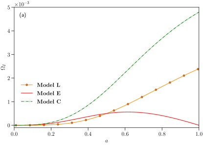
(a)

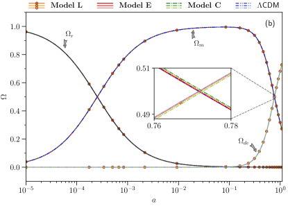
(b)

Figure 1: Plot of (a) the dimensionless interaction parameter $\Omega_{I}$ and (b) density parameter $\Omega$ against scale factor $a$. The x-axis in Fig. (b) is in logarithmic scale The solid line with solid circles represents Model L, solid line represents Model E and dashed-dot line represents Model C while the dashed-dot-dot line is for $\Lambda$CDM. The inset shows the zoomed-in portion for the region $a=0.76$ to $a=0.78$.

III Evolution of perturbations

The perturbed FLRW metric in a general gauge takes the form Kodama and Sasaki (1984); Mukhanov et al. (1992); Ma and Bertschinger (1995)

$$\begin{split}ds^{2}=a^{2}\left(\tau\right)&\left\{-\left(1+2\phi\right)d\tau^{2}+2\,\partial_{i}B\,d\tau\,dx^{i}+\right.\\ &\left.\left[\left(1-2\psi\right)\delta_{ij}+2\partial_{i}\partial_{j}E\right]dx^{i}dx^{j}\right\},\end{split}$$ (12)

where $\phi,\psi,B,E$ are gauge-dependant scalar functions of space and time. In presence of interaction, the covariant form of the energy-momentum conservation equation will be

$$T^{\,\mu\nu}_{\left(A\right);\nu}=Q^{\,\mu}_{\left(A\right)}\,,\hskip 8.5359pt\mbox{where}\hskip 5.69046pt\sum_{A}Q^{\mu}_{\left(A\right)}=0~{}.$$ (13)

The energy-momentum transfer function for the fluid ‘$A$’, $Q^{\,\mu}_{\left(A\right)}$, can be split into the energy transfer rate, $Q_{\left(A\right)}$ and the momentum transfer rate, $F^{\mu}_{\left(A\right)}$, relative to the total $4$-velocity as Väliviita et al. (2008); Majerotto et al. (2010); Clemson et al. (2012)

$$Q^{\,\mu}_{\left(A\right)}=Q_{\left(A\right)}u^{\,\mu}+F^{\,\mu}_{\left(A\right)}\,,\hskip 14.22636ptu_{\mu}F^{\,\mu}_{\left(A\right)}=0\,,\hskip 14.22636ptF^{\,\mu}_{\left(A\right)}=a^{-1}\,\left(0,\partial^{i}\,f_{A}\right).$$ (14)

Writing the total 4-velocity, $u^{\,\mu}$, in terms of the total peculiar velocity, $v$ as

$$u^{\,\mu}=a^{-1}\left(1-\phi,v^{i}\right),$$ (15)

the temporal and spatial components of the 4-energy-momentum transfer rate can be written as

$$Q^{0}_{\left(A\right)} = a^{-1}\,\left[Q_{A}(1-\phi)+\delta Q_{A}\right],$$ (16)

$$\hskip 14.22636pt\mbox{and}\hskip 14.22636ptQ^{i}_{\left(A\right)} = a^{-1}\,\left[Q_{A}\,v^{i}+\partial^{i}\,f_{A}\right]$$ (17)

respectively, where $\delta Q_{A}$ is the perturbation in the energy transfer rate and $f_{A}$ is the momentum transfer potential.

The perturbed conservation equations of the fluid ‘$A$’ in the Fourier space are written as

$$\begin{split}\delta\rho^{\prime}_{A}-3\left(\rho_{A}+p_{A}\right)\psi^{\prime}+&k\left(\rho_{A}+p_{A}\right)\left(v_{A}+E^{\prime}\right)+\\ 3\mathcal{H}\,\left(\delta\rho_{A}+\delta p_{A}\right)=&~{}aQ_{A}\phi+a\delta Q_{A},\end{split}$$ (18)

$$\begin{split}\left[\left(\rho_{A}+p_{A}\right)\left(v_{A}+B\right)\right]^{\prime}+&4\mathcal{H}\left(\rho_{A}+p_{A}\right)\left(v_{A}+B\right)-\\ k\left(\rho_{A}+p_{A}\right)\phi-k\,\delta p_{A}&=aQ_{A}\left(v+B\right)-a\,kf_{A}~{}.\end{split}$$ (19)

In Eqns. (18) and (19), $\delta\rho_{A}$ is the perturbation in the energy density, $\delta p_{A}$ is the perturbation in pressure, $u^{\,\mu}_{A}=a^{-1}\left(1-\phi,v_{A}^{i}\right)$ is the 4-velocity with peculiar velocity $v_{A}$ of the fluid ‘$A$’ and $k$ is the wavenumber. For an adiabatic perturbation, the pressure perturbation Wands et al. (2000); Malik et al. (2003); Malik and Wands (2005); Väliviita et al. (2008); Malik and Wands (2009) in presence of interaction is

$$\delta p_{A}=c_{s,\,A}^{2}\delta\rho_{A}+\left(c_{s,\,A}^{2}-c_{a,\,A}^{2}\right)\left[3\mathcal{H}\left(1+w_{A}\right)\rho_{A}-aQ_{A}\right]\frac{v_{A}}{k},$$ (20)

where $c_{a,\,A}^{2}=\frac{p_{A}^{\prime}}{\rho_{A}^{\prime}}$ is the square of adiabatic sound speed and $c_{s,\,A}^{2}=\frac{\delta p_{A}}{\delta\rho_{A}}$ is the square of effective sound speed in the rest frame of $A$-th fluid.

The dynamical coupling parameter $\beta_{0}$ defined in Eqn. (7) in the previous section is considered to be not affected by perturbation. This assumption is valid for the EoS parameter defined in Eqn. (9) and the Hubble parameter, $\mathcal{H}$. These perturbation equations are solved along with the perturbation equations Kodama and Sasaki (1984); Mukhanov et al. (1992); Ma and Bertschinger (1995) of the radiation, neutrino and baryon using the publicly available Boltzmann code CAMB  Lewis et al. (2000) after suitably modifying it.

Using (15), Eqn. (7) can be conveniently written as

$$Q=\frac{\mathcal{H}\rho_{de}\,\beta\left(a\right)}{a}.$$ (21)

Defining the density contrasts of the dark matter and dark energy as $\delta_{c}=\delta\rho_{c}/\rho_{c}$ and $\delta_{de}=\delta\rho_{de}/\rho_{de}$ respectively and using Eqns. (20) and (21), the perturbation Eqns. (18) and (19) are written in synchronous gauge Ma and Bertschinger (1995) ($\phi=B=0$, $\psi=\eta$ and $k^{2}\,E=-\mathsf{h}/2-3\eta$, where $\eta$ and $\mathsf{h}$ are synchronous gauge fields in the Fourier space) as

$$\delta_{c}^{\prime}+kv_{c}+\frac{\mathsf{h}^{\prime}}{2} = \mathcal{H}\beta\left(a\right)\frac{\rho_{de}}{\rho_{c}}\left(\delta_{c}-\delta_{de}\right),$$ (22)

$$v_{c}^{\prime}+\mathcal{H}v_{c} = 0~{},$$ (23)

$$\begin{split}\delta_{de}^{\prime}+3\mathcal{H}&\left(c_{s,\,de}^{2}-w_{de}\right)\delta_{de}+\left(1+w_{de}\right)\left(kv_{de}+\frac{\mathsf{h}^{\prime}}{2}\right)\\ +3\mathcal{H}&\left[3\mathcal{H}\left(1+w_{de}\right)\left(c_{s,\,de}^{2}-w_{de}\right)\right]\frac{v_{de}}{k}+3\mathcal{H}w_{de}^{\prime}\frac{v_{de}}{k}\\ =\,3\mathcal{H}^{2}&\beta\left(a\right)\left(c_{s,\,de}^{2}-w_{de}\right)\frac{v_{de}}{k},\end{split}$$ (24)

$$v_{de}^{\prime}+\mathcal{H}\left(1-3c_{s,\,de}^{2}\right)v_{de}-\frac{k\,\delta_{de}\,c_{s,\,de}^{2}}{\left(1+w_{de}\right)}=\frac{\mathcal{H}\,\beta\left(a\right)}{\left(1+w_{de}\right)}\,\left[v_{c}-\left(1+c_{s,\,de}^{2}\right)v_{de}\right].$$ (25)

It may be noted that although the interaction term in Eqn. 21 is similar to that used in Kumar et al. (2019), the perturbation equations (Eqns. (23)-(25)) are different from those in Kumar et al. (2019) as we have not considered vacuum energy with $w_{de}=-1$. For the same reason the initial conditions, to follow, are also different in our case. For a detailed discussion on perturbation equations in an inhomogeneous vacuum scenario, we refer to Wands et al. (2012); De-Santiago et al. (2012); Wang et al. (2013); Salvatelli et al. (2014); Martinelli et al. (2019). The coupled differential equations (Eqns. (23)-(25)) are solved with $k=0.1\,h$ $\mbox{Mpc}^{-1}$ and the adiabatic initial conditions using CAMB. Using the gauge-invariant quantity Malik et al. (2003); Malik and Wands (2009); He et al. (2009); Chongchitnan (2009); Xia (2009) $\zeta_{A}=\left(-\psi-\mathcal{H}\frac{\delta\rho_{A}}{\rho_{A}^{\prime}}\right)$ and relative entropy perturbation $S_{AB}=3\left(\zeta_{A}-\zeta_{B}\right)$, the adiabatic initial conditions for $\delta_{c}$, $\delta_{de}$ in presence of interaction are obtained respectively as

$$\delta_{ci} = \left[3+\frac{\rho_{de}}{\rho_{c}}\beta\left(a\right)\right]\frac{\delta_{\gamma}}{3\left(1+w_{\gamma}\right)},$$ (26a)

$$\delta_{dei} = \left[3\,\left(1+w_{de}\right)-\beta\left(a\right)\right]\frac{\delta_{\gamma}}{3\left(1+w_{\gamma}\right)},$$ (26b)

Here, $\delta_{\gamma}$ is the density fluctuation of photons. As can be seen from Eqn. (23), there is no momentum transfer in the DM frame, hence initial value for $v_{c}$ is set to zero ($v_{ci}=0$) Bean et al. (2008); Chongchitnan (2009); Xia (2009); Väliviita et al. (2008). The initial value for the dark energy velocity, $v_{de}$ is assumed to be same as the initial photon velocity, $v_{dei}=v_{\gamma\,i}$. To avoid the instability in dark energy perturbations due to the the propagation speed of pressure perturbations, we have set $c_{s,\,de}^{2}=1$ Hu (1998); Bean and Doré (2004); Gordon and Hu (2004); Afshordi et al. (2005); Väliviita et al. (2008).

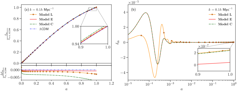
Figure 2: (a) Plot of Upper Panel : the matter density contrast $\frac{\delta_{m}}{\delta_{m\,0,\,\scriptsize{\Lambda\text{CDM}}}}$ and Lower Panel : fractional growth rate is defined as $\frac{\Delta\delta_{m}}{\delta_{m,\,\scriptsize{\Lambda\text{CDM}}}}=\left(1-\frac{\delta_{m}}{\delta_{m,\,\scriptsize{\Lambda\text{CDM}}}}\right)$ relative to the $\Lambda$CDM model against $a$. The origin on the x-axis represents $10^{-5}$. (b) Plot of the dark energy density fluctuation, $\delta_{de}$ against $a$ in logarithmic scale for $k=0.1\,h$ $\mbox{Mpc}^{-1}$. The solid line with solid circles represents Model L, solid line represents Model E and dashed-dot line represents Model C while the dashed-dot-dot line is for $\Lambda$CDM. The inset shows the zoomed-in portion from $a=0.9$ to $a=1.0$.

Figure (2a) shows the variation of the density contrast, $\delta_{m}=\delta\rho_{m}/\rho_{m}$ for the cold dark matter ($c$) taken together and the baryonic matter ($b$) against $a$ for Model L, Model E and Model C along with the $\Lambda$CDM model. For a better comparison with the $\Lambda$CDM model, $\delta_{m}$ is scaled by $\delta_{m0}=\delta_{m}\left(a=1\right)$ of $\Lambda$CDM . As can be seen from the Fig. (2a), the growth of density fluctuation $\delta_{m}$ is similar in all the model at early times. The effect of interaction comes into play at late time. The late-time growth of $\delta_{m}$ (inset of (2a)) shows that Model E agrees well with the $\Lambda$CDM model, whereas Model L and Model C grow to a little higher value. Figure (2b) shows the variation of the dark energy density contrast $\delta_{de}$ for Model L, Model E and Model C. At early time, $\delta_{de}$ oscillates and then decays to very small values. In Model C, the early time evolution of $\delta_{de}$ is similar to Model E while the late time evolution is similar to Model L. To understand the differences among the three models and the $\Lambda$CDM model, we have shown the fractional matter density contrast, $\frac{\Delta\delta_{m}}{\delta_{m,\,\scriptsize{\Lambda\text{CDM}}}}=\left(1-\frac{\delta_{m}}{\delta_{m,\,\scriptsize{\Lambda\text{CDM}}}}\right)$ in the lower panel of Fig. (2a). It is clearly seen that, $\delta_{m}$ for Model E evolves close to the $\Lambda$CDM model.

III.1 Effect on CMB temperature, matter power spectrum and $f\sigma_{8}$

It is necessary to have an insight into other physical quantities like the CMB temperature spectrum, matter power spectrum and the logarithmic growth of matter perturbation, to differentiate the interacting models. The CMB temperature power spectrum is given as

$$C_{\ell}^{TT}=\frac{2}{k}\int k^{2}dk\,P_{\zeta}\left(k\right)\Delta^{2}_{T\ell}\left(k\right),$$ (27)

where $\ell$ is the multipole index, $P_{\zeta}\left(k\right)$ is the primordial power spectrum, $\Delta_{T\ell}\left(k\right)$ is the temperature transfer function and $T$ represents the temperature. For a detailed analysis on the CMB spectrum we refer to Hu and Sugiyama (1995); Seljak and Zaldarriaga (1996); Dodelson (2003). The matter power spectrum is written as

$$P\left(k,a\right)=A_{s}\,k^{n_{s}}T^{2}\left(k\right)D^{2}\left(a\right),$$ (28)

where $A_{s}$ is the scalar primordial power spectrum amplitude, $n_{s}$ is the spectral index, $T\left(k\right)$ is the matter transfer function and $D\left(a\right)=\frac{\delta_{m}\left(a\right)}{\delta_{m}\left(a=1\right)}$ is the normalised density contrast. For a detailed description we refer to Dodelson (2003). Both $C_{\ell}^{TT}$ and $P\left(k,a\right)$ are computed numerically using CAMB. The values of power spectrum amplitude, $A_{s}=2.100549\times 10^{-9}$ and spectral index, $n_{s}=0.9660499$ are taken from Planck 2018 data Aghanim et al. (2020a).

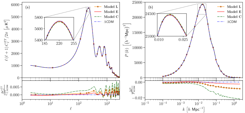
Figure 3: Upper Panel : (a) Plot of CMB temperature power spectrum in units of $\mu\mbox{K}^{2}$ with the multipole index $\ell$ in logarithmic scale. (b) Plot of matter power spectrum $P\left(k\right)$ in units of $\left(h^{-1}\mbox{Mpc}\right)^{3}$ with wavenumber $k$ in units of $h\,\mbox{Mpc}^{-1}$. Lower Panel : Plot of fractional change in the temperature spectrum, $\frac{\Delta C_{\ell}^{TT}}{C_{\ell,\,\scriptsize{\Lambda\text{CDM}}}^{TT}}=\left(1-\frac{C_{\ell}^{TT}}{C_{\ell,\,\scriptsize{\Lambda\text{CDM}}}^{TT}}\right)$ and the fractional change in matter power spectrum, $\frac{\Delta P}{P_{\scriptsize{\Lambda\text{CDM}}}}=\left(1-\frac{P}{P_{\scriptsize{\Lambda\text{CDM}}}}\right)$. For both the panels, the solid line with solid circles represents Model L, solid line represents Model E and dashed-dot line represents Model C while the dashed-dot-dot line is for $\Lambda$CDM at $a=1$. The inset shows the zoomed-in versions of the peaks.

Figure (3) shows the temperature and matter power spectrum for Model L, Model E, Model C and $\Lambda$CDM at $a=1$. In Model L and Model C, more matter content results in lower amplitude of the first peak of the CMB spectrum compared to the $\Lambda$CDM model. The lower panel of Fig. (3a), shows the fractional change ($=\Delta C_{\ell}^{TT}/C_{\ell,\,\scriptsize{\Lambda\text{CDM}}}^{TT}$) in $C_{\ell}^{TT}$. It is seen from the lower panel of Fig. (3a), that the low-$\ell$ modes of Model E increases through the integrated Sachs-Wolfe (ISW) effect. More matter content also increases the matter power spectrum compared to the $\Lambda$CDM model. The deviations from the $\Lambda$CDM model are prominent for the smaller modes. These features are clear from the lower panel of Fig. (3b), which shows the fractional change in matter power spectrum, $\Delta P/P_{\scriptsize{\Lambda\text{CDM}}}$ of the interacting models relative to the $\Lambda$CDM model.

The presence of the interaction modifies the logarithmic growth rate which helps in differentiating between the models even better. The growth rate is the logarithmic derivative of the density fluctuation of matter (baryon and CDM) and is written as

$$f\left(a\right)=\frac{d\ln\delta_{m}}{d\ln a}~{}=~{}a\frac{d}{d\,a}\left(\frac{\delta\rho_{m}}{\rho_{m}}\right).$$ (29)

Since, $\delta\rho_{m}=\left(\delta_{c}\rho_{c}+\delta_{b}\rho_{b}\right)$, $\delta_{b}$ being the baryon density fluctuation, in presence of interaction the growth rate Costa et al. (2017) will be

$$f\left(a\right)=a\left(\frac{\delta_{c,\,a}\,\,\rho_{c}+\delta_{b,\,a}\,\,\rho_{b}}{\delta_{m}\,\rho_{m}}-\frac{aQ\,\delta_{c}}{\delta_{m}\,\rho_{m}}-\frac{aQ}{\rho_{m}}\right),$$ (30)

where ‘${}_{,\,a}$’ denotes the derivative with respect to the scale factor $a$ and $Q$ is given by Eqn. (21). It must be noted that the last two terms involving interaction $Q$ is introduced in Eqn. (30) via the evolution of $\rho_{c}$ (Eqns. (4)). We have calculated the growth rate, $f$ for the different models using CAMB.

Observationally the galaxy density fluctuation, $\delta_{g}$ is measured, which in turn gives the matter density fluctuation, $\delta_{m}$ as $\delta_{g}=b\delta_{m}$, where $b\in\left[1,3\right]$ is the bias parameter. This $\delta_{m}$ is used to calculate the logarithmic growth rate, $f$. Thus, $f$ is sensitive to $b$ and is not a very reliable quantity. A more dependable observational quantity is defined as the product $f\left(a\right)\sigma_{8}\left(a\right)$ Percival and White (2009), where $\sigma_{8}\left(a\right)$ is the root-mean-square (rms) mass fluctuations within the sphere of radius $R=8h^{-1}\,\mbox{Mpc}$. The mean-square mass fluctuation is given by

$$\sigma^{2}\left(R,z\right)=\frac{1}{2\pi^{2}}\int k^{3}P\left(k,z\right)W\left(kR\right)^{2}\frac{dk}{k}$$ (31)

where $P\left(k,z\right)$ is the power spectrum given in Eqn. (28) and $W\left(kR\right)$ is the top-hat window function given by

$$W\left(kR\right)=3\left[\frac{\sin\left(kR\right)}{\left(kR\right)^{3}}-\frac{\cos\left(kR\right)}{\left(kR\right)^{2}}\right].$$ (32)

When the size of the filter is $R=8h^{-1}\,\mbox{Mpc}$, $\sigma^{2}\left(R,z\right)\equiv\sigma_{8}^{2}\left(z\right)$. The rms linear density fluctuation is also written as $\sigma_{8}\left(a\right)=\sigma_{8}\left(1\right)\frac{\delta_{m}\left(a\right)}{\delta_{m}\left(1\right)}$, where $\sigma_{8}\left(1\right)$ and $\delta_{m}\left(1\right)$ are the values at $a=1$, and $f$ and $\sigma_{8}\left(1\right)$ for the different models are obtained from Eqn. (30) and (31) using our modified version of CAMB. The combination $f\sigma_{8}$ is written as

$$f\sigma_{8}\left(a\right)\equiv f\left(a\right)\sigma_{8}\left(a\right)=\sigma_{8}\left(1\right)\frac{a}{\delta_{m}\left(1\right)}\frac{d\delta_{m}}{d\,a}.$$ (33)

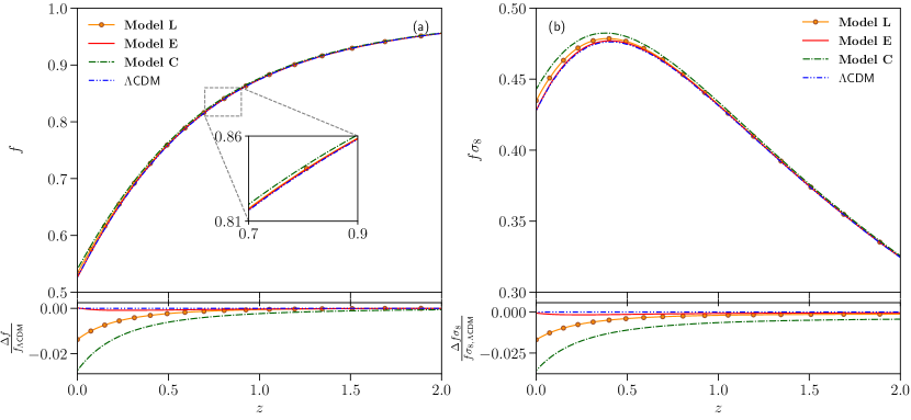
Figure 4: Upper Panel : Plot of (a) linear growth rate $f$ and (b) $f\sigma_{8}$ against redshift $z$. The inset shows the zoomed-in portion from $z=0.7$ to $z=0.9$. Lower Panel : Plot of fractional change in the temperature spectrum, $\frac{\Delta f}{f_{\scriptsize{\Lambda\text{CDM}}}}=\left(1-\frac{f}{f_{\scriptsize{\Lambda\text{CDM}}}}\right)$ and the fractional change in matter power spectrum, $\frac{\Delta f\sigma_{8}}{f\sigma_{8,\,\scriptsize{\Lambda\text{CDM}}}}=\left(1-\frac{f\sigma_{8}}{f\sigma_{8,\,\scriptsize{\Lambda\text{CDM}}}}\right)$. For both the panels, the solid line with solid circles represents Model L, solid line represents Model E and dashed-dot line represents Model C while the dashed-dot-dot line is for $\Lambda$CDM.

The logarithmic growth rates, $f$ and $f\sigma_{8}$ are independent of the wavenumber $k$ for smaller redshift, $z$, so only the domain $z=0$ to $z=2$ is considered here. The redshift, $z$ and the scale factor $a$ are related as $z=\frac{a_{0}}{a}-1$, $a_{0}$ being the present value (taken to be unity). The difference in the models is magnified in the $f$ and $f\sigma_{8}$ analysis. As can be seen from Fig. (4), growth rates ($f$) and $f\sigma_{8}$ are different for the different models in the recent past. The differences due to the evolution of interaction are seen in $f$ and $f\sigma_{8}$. Both Model L and Model C have slightly higher values of $f$ and $f\sigma_{8}$ at $z=0$, compared to the value obtained from the $\Lambda$CDM model. For Model E and the $\Lambda$CDM model, the values of $f$ and $f\sigma_{8}$ are same at $z=0$. When the energy transfer rates were different in the recent past, Model E had a slightly larger value of $f$ and $f\sigma_{8}$ (compared to the $\Lambda$CDM model) when the interaction was non-zero. The fractional changes in growth rate ($\Delta f/f_{\scriptsize{\Lambda\text{CDM}}}$) and $f\sigma_{8}$ ($\Delta f\sigma_{8}/f\sigma_{8,\,\scriptsize{\Lambda\text{CDM}}}$) of the interacting models relative to the $\Lambda$CDM model are shown in the lower panels. The difference among the three models is distinctly seen.

IV Observational Constraints

In this section, Model L, Model E and Model C are tested against observational datasets like the CMB, BAO, Supernovae and RSD data by using the Markov Chain Monte Carlo (MCMC) analysis of the publicly available, efficient MCMC simulator CosmoMC  Lewis (2013); Lewis and Bridle (2002). The datasets and the methodology are discussed in the Appendix A. The datasets are used to constrain the nine-dimensional parameter space given as

$$P\equiv\{\Omega_{b}h^{2},\Omega_{c}h^{2},100\theta_{MC},\tau,\beta_{0},w_{0},w_{1},\ln\left(10^{10}A_{s}\right),n_{s}\},$$ (34)

where $\Omega_{b}h^{2}$ is the baryon density, $\Omega_{c}h^{2}$ is the cold dark matter density, $\theta_{MC}$ is the angular acoustic scale, $\tau$ is the optical depth, $\beta_{0}$, $w_{0}$ and $w_{1}$ are the free model parameters, $A_{s}$ is the scalar primordial power spectrum amplitude and $n_{s}$ is the scalar spectral index. The parameter space, $P$, for all the three models, is explored for the flat prior ranges given in Table 2. We allowed the prior of $\beta_{0}$ to cross the zero and set the prior of $w_{0}$ and $w_{1}$ such that such that $w_{de}$ is always in the quintessence region.

Table 2: Prior ranges of nine independent parameters used in the CosmoMC analysis.

Parameter	Prior
$\Omega_{b}h^{2}$	$\left[0.005,0.1\right]$
$\Omega_{c}h^{2}$	$\left[0.001,0.99\right]$
$100\theta_{MC}$	$\left[0.5,10\right]$
$\tau$	$\left[0.01,0.8\right]$
$\beta_{0}$	$\left[-1.0,1.0\right]$
$w_{0}$	$\left[-0.9999,-0.3333\right]$
$w_{1}$	$\left[0.005,1.0\right]$
$\ln\left(10^{10}A_{s}\right)$	$\left[1.61,3.91\right]$
$n_{s}$	$\left[0.8,1.2\right]$

IV.1 Model L

For Model L, the marginalised values with errors at $1\sigma$ ($68\%$ confidence level) of the nine free parameters and three derived parameters, $H_{0}$, $\Omega_{m}$ and $\sigma_{8}$, are listed in Table 3. Henceforth, the 1D marginalised values given in the tables will be referred to as mean values. The correlations between the model parameters ($\beta_{0}$, $w_{0}$, $w_{1}$) and the derived parameters ($H_{0}$, $\Omega_{m}$, $\sigma_{8}$) and their marginalised contours are shown in Fig. 5. The contours contain $1\sigma$ region ($68\%$ confidence level) and $2\sigma$ region ($95\%$ confidence level). When only the Planck data is considered, the mean value of the coupling parameter, $\beta_{0}(=0.00788^{+0.00815+0.0158}_{-0.00815-0.0162})$, is positive with zero in the $1\sigma$ region indicating energy transfers from DM to DE. The parameters $w_{0}(<-0.909<-0.800)$ and $w_{1}(<0.174<0.365)$ remain unconstrained even in the $2\sigma$ region. For other parameters, the mean values are compared with their $\Lambda$CDM counterparts from the Planck estimation Aghanim et al. (2020a). The Hubble expansion rate, $H_{0}$, is obtained at a value lower than $67.36\pm 0.54$ in $\mbox{km s}^{-1}\mbox{Mpc}^{-1}$, as obtained for the $\Lambda$CDM model Aghanim et al. (2020a). Though the mean value is lower than that obtained from the Planck estimate, the presence of high error bars results in $3.5\sigma$ tension with the local measurement as $H_{0}=74.03\pm 1.42$ $\mbox{km s}^{-1}\mbox{Mpc}^{-1}$. The value of the late time clustering amplitude ($\sigma_{8}$) is skewed towards the value, $\sigma_{8}=0.77^{+0.04}_{-0.03}$, as obtained by the galaxy cluster counts using thermal Sunyaev-Zel’dovich (tSZ) signature Aghanim et al. (2020a); Zubeldia and Challinor (2019). Thus, Planck data alone alleviates the $\sigma_{8}$ tension in the Model L. Figure 5 highlights the positive correlation between $H_{0}$ and $\sigma_{8}$ and strong negative correlations of $\Omega_{m}$ with $H_{0}$ and $\sigma_{8}$. The parameter $w_{0}$ has negative correlations with $w_{1}$, $H_{0}$ and $\sigma_{8}$ and positive correlation with $\Omega_{m}$. The coupling parameter ($\beta_{0}$) is uncorrelated to the others.

Addition of the BAO to the Planck data, increases the value of $\beta_{0}$ to $0.00814^{+0.00755+0.0146}_{-0.00755-0.0151}$ with zero outside the $1\sigma$ region. The Planck and BAO combination cannot constrain the parameters $w_{0}$ and $w_{1}$. The mean value of the Hubble parameter increases considerably but is still smaller than the corresponding value for $\Lambda$CDM, $H_{0}=67.66\pm 0.42$ in $\mbox{km s}^{-1}\mbox{Mpc}^{-1}$ in the $1\sigma$ region. The considerable decrease in error bar increased the $H_{0}$ tension to $\sim 4\sigma$. The values of $\Omega_{m}$ decreases and $\sigma_{8}$ increases and are higher than the $\Lambda$CDM counterpart ($\Omega_{m}=0.3111\pm 0.0056$ and $\sigma_{8}=0.8102\pm 0.006$) in the $1\sigma$ region. Thus, addition of the BAO data to the Planck data restores the $\sigma_{8}$ tension ($\sim 0.79\sigma$) in Model L. The combination also lowers the error regions substantially.

Interestingly, addition of $f\sigma_{8}$ to the Planck data changes the parameter mean values in the similar fashion like the Planck and BAO combination but the error bars become higher. This is also clear from Fig. 5. The mean value of $\beta_{0}(=0.00752^{+0.00757+0.0145}_{-0.00757-0.0151})$ is smaller the Planck and BAO combination. Clearly, addition of the $f\sigma_{8}$ data restores the $\sigma_{8}$ tension in Model L.

Addition of the BAO and Pantheon to the Planck data, increases the mean value of $\beta_{0}(=0.00859^{+0.00745+0.0145}_{-0.00745-0.0148})$ with zero in the $2\sigma$ region. The parameters $w_{0}$ and $w_{1}$ still remain unconstrained. The combination increases the $H_{0}$ mean value but is still slightly smaller than the fiducial $\Lambda$CDM value. The central value of $\Omega_{m}$ at the present epoch remains slightly larger whereas $\sigma_{8}$ remains slightly smaller than the $\Lambda$CDM case. Clearly, the $\sigma_{8}$ tension is restored.

Combining $f\sigma_{8}$ data with Planck, BAO and Pantheon lowers the mean values of both $\Omega_{m}$ and $\sigma_{8}$ but increases the value of $H_{0}$ compared to the baseline Planck values Aghanim et al. (2020a). Thus, addition of all the datasets worsen the $H_{0}$ tension ($\sim 4.2\sigma$) and the $\sigma_{8}$ tension ($\sim 0.87\sigma$). The mean value of $\beta_{0}(=0.00818^{+0.00731+0.0142}_{-0.00731-0.0146})$ decreases slightly with zero in the $2\sigma$ region. Although the constraints on $w_{0}$ and $w_{1}$ tightens, they still remain unconstrained.

Combination of all the datasets significantly reduced the error bars. The parameters, $\beta_{0}$ and $w_{1}$ become very weakly correlated with other parameters. However, the correlations among the rest of the parameters remain unchanged.

Table 3: Observational constraints on the nine dependent model parameters with three derived parameters separated by a horizontal line and the error bars correspond to $68\%$ confidence level for Model L, using different observational datasets.

Parameter Planck Planck + $f\sigma_{8}$ Planck + BAO Planck + BAO + Pantheon Planck + BAO + Pantheon + $f\sigma_{8}$ $\Omega_{b}h^{2}$ $0.022362\pm 0.000168$ $0.022483\pm 0.000163$ $0.022487\pm 0.000156$ $0.022500\pm 0.000154$ $0.022542\pm 0.000152$ $\Omega_{c}h^{2}$ $0.12005\pm 0.00129$ $0.11853\pm 0.00117$ $0.11848\pm 0.00102$ $0.118381\pm 0.000977$ $0.117838\pm 0.000927$ $100\theta_{MC}$ $1.040773\pm 0.000326$ $1.040938\pm 0.000316$ $1.040951\pm 0.000315$ $1.040954\pm 0.000316$ $1.041007\pm 0.000313$ $\tau$ $0.05475\pm 0.00773$ $0.05641^{+0.00705}_{-0.00794}$ $0.05732^{+0.00701}_{-0.00787}$ $0.05707^{+0.00691}_{-0.00777}$ $0.05791\pm 0.00760$ $\beta_{0}$ $0.00788\pm 0.00815$ $0.00752\pm 0.00757$ $0.00814\pm 0.00755$ $0.00859\pm 0.00745$ $0.00818\pm 0.00731$ $w_{0}$ $<-0.909$ $<-0.976$ $<-0.968$ $<-0.980$ $<-0.985$ $w_{1}$ $<0.174$ $<0.0672$ $<0.0707$ $<0.0623$ $<0.0500$ ${\rm{ln}}(10^{10}A_{s})$ $3.0489\pm 0.0149$ $3.0489\pm 0.0147$ $3.0512\pm 0.0148$ $3.0507\pm 0.0145$ $3.0512\pm 0.0146$ $n_{s}$ $0.96330\pm 0.00444$ $0.96672\pm 0.00436$ $0.96674\pm 0.00413$ $0.96690\pm 0.00418$ $0.96818\pm 0.00412$ $H_{0}\left[\mbox{km s}^{-1}\mbox{Mpc}^{-1}\right]$ $63.98^{+2.45}_{-1.47}$ $66.93^{+1.04}_{-0.719}$ $66.770^{+0.792}_{-0.602}$ $67.179^{+0.579}_{-0.521}$ $67.596\pm 0.524$ $\Omega_{m}$ $0.3507^{+0.0157}_{-0.0292}$ $0.31643^{+0.00846}_{-0.0116}$ $0.31778^{+0.00681}_{-0.00832}$ $0.31368\pm 0.00632$ $0.30871\pm 0.00598$ $\sigma_{8}$ $0.7825^{+0.0228}_{-0.0141}$ $0.8027^{+0.0102}_{-0.00836}$ $0.8020^{+0.0104}_{-0.00892}$ $0.80541\pm 0.00862$ $0.80560\pm 0.00803$

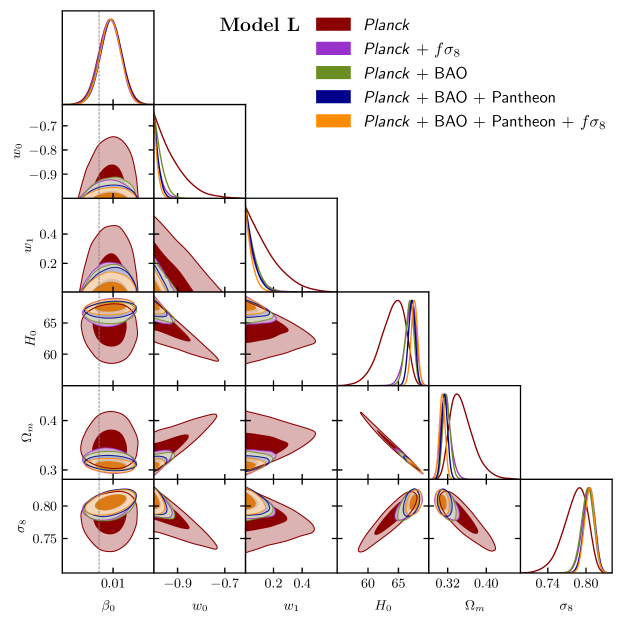
Figure 5: Plot of 1-dimensional marginalised posterior distributions and 2-dimensional marginalised constraint contours on the parameters of Model L containing $68\%$ and $95\%$ probability. The dashed line represents the $\beta_{0}=0$ value.

IV.2 Model E

For Model E, the mean values with $1\sigma$ errors of the nine free parameters along with the three derived parameters, $H_{0}$, $\Omega_{m}$ and $\sigma_{8}$, are given in Table 4. The correlations of the model parameters ($\beta_{0}$, $w_{0}$, $w_{1}$) with the derived parameters ($H_{0}$, $\Omega_{m}$, $\sigma_{8}$) and their marginalised contours are shown in Fig. 6. When only Planck data is considered, the mean value of $\beta_{0}(=0.0339^{+0.0372+0.0724}_{-0.0372-0.0746})$ is large compared to that in Model L, though $\beta_{0}=0$ remains within the $1\sigma$ region. The CPL parameters, $w_{0}(<-0.914<-0.809)$ and $w_{1}(<0.168<0.355)$, remain unconstrained even within the $2\sigma$ region. The values of $H_{0}$ is greater and that of $\sigma_{8}$ is slightly grater whereas $\Omega_{m}$ is slightly lower than those in Model L. Similar to Model L, the discrepancy in the value of $H_{0}$ with the local measurement is at $3.5\sigma$. In Model E also, the Planck data alleviates the $\sigma_{8}$ tension. The distinguishing feature of Model E is that the mean value of $\beta_{0}$ is greater than that obtained in Model L for all the dataset combinations.

Addition of the BAO to the Planck data, increases the mean value of $\beta_{0}(=0.0432^{+0.0376+0.0733}_{-0.0376-0.0744})$ with zero allowed in the $2\sigma$ region. The parameters $w_{0}$ and $w_{1}$ remain unconstrained. The mean value of $H_{0}$ increases considerably but is still smaller than the corresponding value for $\Lambda$CDM. The values of $\Omega_{m}$ decreases and $\sigma_{8}$ increases and are higher than the $\Lambda$CDM counterpart. The addition of BAO data to Planck data restores the $H_{0}$ ($\sim 4\sigma$) and $\sigma_{8}$ ($\sim 0.77\sigma$) tensions in Model E. The combination also lowers the error bars considerably.

Similar to Model L, addition of $f\sigma_{8}$ to the Planck data changes the parameter mean values like the Planck + BAO combination but the error bars still remain a little higher. This is also clear from Fig. 6. The mean value of $\beta_{0}(=0.0395^{+0.0381+0.0735}_{-0.0381-0.0750})$ is slightly smaller than the Planck + BAO combination. The $H_{0}$ and $\sigma_{8}$ tensions are restored on addition of $f\sigma_{8}$ to the Planck data.

Combining BAO and Pantheon with Planck data increases the mean value of $\beta_{0}(=0.0448^{+0.0377+0.0738}_{-0.0377-0.0733})$ and $\beta_{0}=0$ is within the $2\sigma$ region. The Planck + BAO + Pantheon results in a very small change in the mean values of the parameters along with reduced error bars. The mean values of $H_{0}$ and $\sigma_{8}$ increase and $\Omega_{m}$ decreases relative to the Planck + BAO combination. Again, the $\sigma_{8}$ tensions are not alleviated.

Addition of $f\sigma_{8}$ to the combination Planck + BAO + Pantheon, increases the mean value of $H_{0}$ slightly and decreases the mean value of $\Omega_{m}$ very slightly keeping $\sigma_{8}$ almost unchanged. The mean value of $\beta_{0}(=0.0446^{+0.0370+0.0724}_{-0.0370-0.0726})$ decreases slightly with zero in the $2\sigma$ region. Clearly, the addition of datasets do not improve the $H_{0}$ and $\sigma_{8}$ tension in Model E. Addition of the datasets significantly reduces the error bars. The correlations between the parameters for Model E remain same as in Model L.

Table 4: Observational constraints on the nine dependent model parameters with three derived parameters separated by a horizontal line and the error bars correspond to $68\%$ confidence level for Model E, using different observational datasets.

Parameter Planck Planck + $f\sigma_{8}$ Planck + BAO Planck + BAO + Pantheon Planck + BAO + Pantheon + $f\sigma_{8}$ $\Omega_{b}h^{2}$ $0.022358\pm 0.000165$ $0.022490\pm 0.000162$ $0.022489\pm 0.000156$ $0.022500\pm 0.000152$ $0.022546\pm 0.000151$ $\Omega_{c}h^{2}$ $0.12008\pm 0.00126$ $0.11848\pm 0.00117$ $0.11850\pm 0.00101$ $0.118405\pm 0.000970$ $0.117845\pm 0.000909$ $100\theta_{MC}$ $1.040769\pm 0.000324$ $1.040941\pm 0.000318$ $1.040941\pm 0.000313$ $1.040945\pm 0.000315$ $1.040999\pm 0.000313$ $\tau$ $0.05466^{+0.00699}_{-0.00779}$ $0.05630^{+0.00703}_{-0.00797}$ $0.05704^{+0.00704}_{-0.00792}$ $0.05697\pm 0.00749$ $0.05778^{+0.00700}_{-0.00790}$ $\beta_{0}$ $0.0339\pm 0.0372$ $0.0395\pm 0.0381$ $0.0432\pm 0.0376$ $0.0448\pm 0.0377$ $0.0446\pm 0.0370$ $w_{0}$ $<-0.914$ $<-0.977$ $<-0.969$ $<-0.981$ $<-0.985$ $w_{1}$ $<0.168$ $<0.0645$ $<0.0707$ $<0.0604$ $<0.0489$ ${\rm{ln}}(10^{10}A_{s})$ $3.0486\pm 0.0147$ $3.0488\pm 0.0148$ $3.0509\pm 0.0148$ $3.0507\pm 0.0144$ $3.0511\pm 0.0146$ $n_{s}$ $0.96315\pm 0.00453$ $0.96681\pm 0.00434$ $0.96652\pm 0.00419$ $0.96672\pm 0.00418$ $0.96802\pm 0.00404$ $H_{0}\left[\mbox{km s}^{-1}\mbox{Mpc}^{-1}\right]$ $64.12^{+2.40}_{-1.39}$ $67.00^{+1.02}_{-0.702}$ $66.787^{+0.775}_{-0.600}$ $67.200^{+0.577}_{-0.516}$ $67.631\pm 0.516$ $\Omega_{m}$ $0.3492^{+0.0149}_{-0.0282}$ $0.31569^{+0.00834}_{-0.0114}$ $0.31765^{+0.00678}_{-0.00812}$ $0.31353^{+0.00590}_{-0.00658}$ $0.30842\pm 0.00588$ $\sigma_{8}$ $0.7836^{+0.0221}_{-0.0138}$ $0.80265^{+0.00992}_{-0.00800}$ $0.8019^{+0.0102}_{-0.00866}$ $0.80539\pm 0.00830$ $0.80573\pm 0.00774$

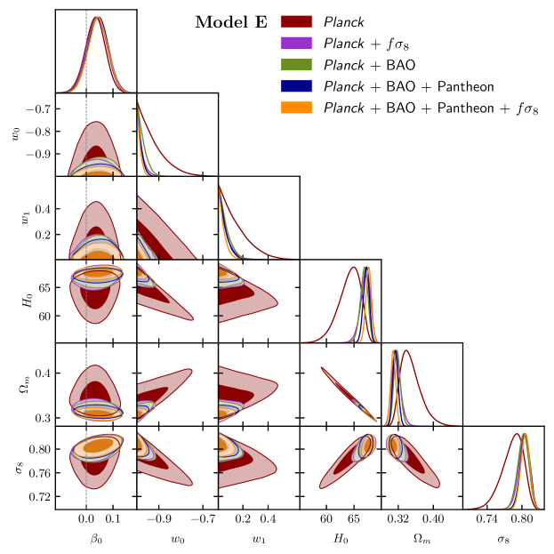
Figure 6: Plot of 1-dimensional marginalised posterior distributions and 2-dimensional marginalised constraint contours on the parameters of Model E containing $68\%$ and $95\%$ probability. The dashed line represents the $\beta_{0}=0$ value.

IV.3 Model C

The mean values of the parameters with $1\sigma$ errors for Model C are given in Table 5. In Table 5, the mean values and $1\sigma$ errors of the three derived parameters, $H_{0}$, $\Omega_{m}$ and $\sigma_{8}$, are also quoted. The correlations between the model parameters ($\beta_{0}$, $w_{0}$, $w_{1}$) and the derived parameters ($H_{0}$, $\Omega_{m}$, $\sigma_{8}$) along with their marginalised contours are shown in Fig. 7. The parameter values of Model C are very close to those of Model L and they respond to the datasets in the similar fashion as well. Similar to Model L and Model E, $H_{0}$ tension is at $\sim 4\sigma$ and only the Planck data alleviates the $\sigma_{8}$ tension in Model C whereas consideration of other datasets restore the tension. The main difference is that the mean values of $\beta_{0}$ in Model C is slightly smaller than that in Model L. These features are clearly seen from Table 5.

Table 5: Observational constraints on the nine dependent model parameters with three derived parameters separated by a horizontal line and the error bars correspond to $68\%$ confidence level for Model C, using different observational datasets.

Parameter Planck Planck + $f\sigma_{8}$ Planck + BAO Planck + BAO + Pantheon Planck + BAO + Pantheon + $f\sigma_{8}$ $\Omega_{b}h^{2}$ $0.022358\pm 0.000164$ $0.022482\pm 0.000164$ $0.022487\pm 0.000156$ $0.022499\pm 0.000151$ $0.022545\pm 0.000152$ $\Omega_{c}h^{2}$ $0.12007\pm 0.00128$ $0.11854\pm 0.00118$ $0.11849\pm 0.00100$ $0.118388\pm 0.000977$ $0.117824\pm 0.000935$ $100\theta_{MC}$ $1.040772\pm 0.000322$ $1.040939\pm 0.000321$ $1.040947\pm 0.000314$ $1.040954\pm 0.000312$ $1.041011\pm 0.000311$ $\tau$ $0.05491\pm 0.00757$ $0.05638^{+0.00708}_{-0.00788}$ $0.05718^{+0.00685}_{-0.00788}$ $0.05730\pm 0.00751$ $0.05800^{+0.00707}_{-0.00790}$ $\beta_{0}$ $0.00624\pm 0.00673$ $0.00621\pm 0.00626$ $0.00696\pm 0.00629$ $0.00708\pm 0.00631$ $0.00693\pm 0.00615$ $w_{0}$ $<-0.907$ $<-0.977$ $<-0.969$ $<-0.981$ $<-0.985$ $w_{1}$ $<0.174$ $<0.0681$ $<0.0728$ $<0.0610$ $<0.0511$ ${\rm{ln}}(10^{10}A_{s})$ $3.0493\pm 0.0146$ $3.0489\pm 0.0147$ $3.0511\pm 0.0146$ $3.0511\pm 0.0144$ $3.0514\pm 0.0147$ $n_{s}$ $0.96331\pm 0.00444$ $0.96670\pm 0.00435$ $0.96670\pm 0.00416$ $0.96695\pm 0.00415$ $0.96823\pm 0.00414$ $H_{0}\left[\mbox{km s}^{-1}\mbox{Mpc}^{-1}\right]$ $63.93^{+2.51}_{-1.44}$ $66.93^{+1.03}_{-0.714}$ $66.759^{+0.795}_{-0.594}$ $67.187^{+0.581}_{-0.516}$ $67.606^{+0.552}_{-0.493}$ $\Omega_{m}$ $0.3513^{+0.0153}_{-0.0299}$ $0.31643^{+0.00843}_{-0.0115}$ $0.31789^{+0.00671}_{-0.00832}$ $0.31361\pm 0.00631$ $0.30860\pm 0.00605$ $\sigma_{8}$ $0.7821^{+0.0232}_{-0.0140}$ $0.8026^{+0.0100}_{-0.00823}$ $0.8020^{+0.0104}_{-0.00879}$ $0.80558\pm 0.00856$ $0.80564\pm 0.00807$

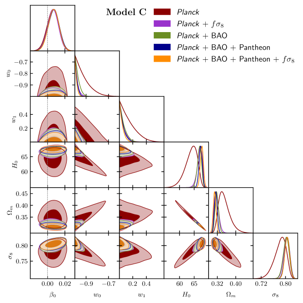
Figure 7: Plot of 1-dimensional marginalised posterior distributions and 2-dimensional marginalised constraint contours on the parameters of Model C containing $68\%$ and $95\%$ probability. The dashed line represents the $\beta_{0}=0$ value.

Tension in the $H_{0}$ parameter:

Dark energy interacting with dark matter is a plausible scenario to resolve the $H_{0}$ tension. When $Q>0$, energy flows from dark matter to dark energy, and we have less dark matter in the present epoch than in the uncoupled case. The locations and heights of the peaks and troughs in the CMB anisotropy depend on the combination $\Omega_{m}h^{2}$ of the present epoch. Since baryon energy density remains unaffected by the interaction, any change in the matter (which is a combination of baryonic matter and dark matter) density comes from the dark matter density. For low matter density with fixed $H_{0}$, the heights of the CMB peaks are higher (for details we refer to Dodelson (2003)). So a model with less $\Omega_{c}$ at the present epoch will need to have a higher value of $H_{0}$ so as to keep the heights of the CMB peaks unaltered. Thus a larger value of $H_{0}$ will be obtained when constrained with the CMB data, which will reconcile the $H_{0}$ tension. It may be noted that in the present work, the uncoupled case is not the $\Lambda$CDM model and $H_{0}$ tension is not alleviated.

V Bayesian Evidence

Finally, we aim to investigate which one of Model L, Model E and Model C is statistically favoured by the observational data. The Bayesian evidence or more precisely, the logarithm of the Bayes factor, $\ln B_{ij}$ given in Eqn. (B.3), for each of the three models is calculated. Here, $i$ corresponds to Model L, Model E and Model C for each of the the dataset combination, $j$ corresponds to the reference model, $M_{j}$. The details on the Bayes factor, $B_{ij}$, are discussed in Appendix B. The fiducial $\Lambda$CDM model is considered to be the reference model, and therefore, a negative value ($\ln B_{ij}<0$) indicates a preference for the $\Lambda$CDM model. The logarithmic Bayes factor, $\ln B_{ij}$, is calculated directly from the MCMC chains using the publicly available cosmological package MCEvidence  Heavens et al. (2017a, b). The computed values of $\ln B_{ij}$ for Model L, Model E and Model C are summarised in Table 6. From Table 6, it is clear that the $\Lambda$CDM model is preferred over the interacting models by all the dataset combinations. However, the motive is to assess if there is any observationally preferable evolution stage when the interaction is significant. As can be seen from the relative differences of $\lvert\ln B_{ij}\rvert$ (values corresponding to column $\Delta\ln B_{ij}$) in Table 6), when compared with Model C, Model L is strongly disfavoured while Model E is weakly disfavoured by observational data over Model C.

Table 6: The values of $\ln B_{ij}$, where $j$ is the $\Lambda$CDM model and $i$ is the interacting model. A negative sign indicates $M_{j}$ is favoured over $M_{i}$. The $\lvert\ln B_{ij}\rvert$ values are compared with Table B.1. The column $\Delta\ln B_{ij}$ corresponds to the comparison of Model L and Model E with Model C.

Model	Dataset	$\ln B_{ij}$	$\Delta\ln B_{ij}$
Model L	Planck	$-8.843$	$-2.244$
	Planck + $f\sigma_{8}$	$-11.410$	$-2.245$
	Planck + BAO	$-10.610$	$-2.187$
	Planck + BAO + Pantheon	$-11.354$	$-2.104$
	Planck + BAO + Pantheon + $f\sigma_{8}$	$-11.977$	$-2.328$
Model E	Planck	$-7.233$	$-0.633$
	Planck + $f\sigma_{8}$	$-9.730$	$-0.566$
	Planck + BAO	$-9.047$	$-0.624$
	Planck + BAO + Pantheon	$-9.733$	$-0.483$
	Planck + BAO + Pantheon + $f\sigma_{8}$	$-10.192$	$-0.542$
Model C	Planck	$-6.599$	0.0
	Planck + $f\sigma_{8}$	$-9.164$	0.0
	Planck + BAO	$-8.423$	0.0
	Planck + BAO + Pantheon	$-9.250$	0.0
	Planck + BAO + Pantheon + $f\sigma_{8}$	$-9.650$	0.0

VI Summary and Discussion

The present work deals with the matter perturbations in a cosmological model where the dark energy has an interaction with the dark matter. We investigate the possibility whether the coupling parameter between the two dark components can evolve. We have considered two new examples, (a) the interaction is a recent phenomenon (Model L; Eqn. (8a)), and (b) the interaction is an early phenomenon (Model E; Eqn. (8b)) and compared them with the normally talked about model where the coupling is a constant (Model C; Eqn. (8c)), in the context of density perturbations. The results are compared with the standard $\Lambda$CDM model as well. The rate of energy transfer is proportional to the dark energy density, $\rho_{de}$ and energy flows from dark matter to dark energy. The interaction term is given by Eqn. (21). We have also considered the dark energy to have a dynamical EoS parameter, $w_{de}$ being given by the CPL parametrisation (Eqn. (9)).

We have worked out a detailed perturbation analysis of the models in the synchronous gauge and compared them with each other. The background dynamics of the three interacting models are almost the same, which is evident from the smallness of the coupling parameter and the domination of dark energy at late times. The signature of the presence of interaction at different epochs for different couplings are noticeable in the perturbation analysis.

In all the three interacting models, the fractional density perturbation of dark matter is marginally higher than that in a $\Lambda$CDM model, indicating more clumping of matter. From the CMB temperature spectrum, matter power spectrum and the evolution of growth rate, we note that the presence of interaction for a brief period in the evolutionary history (Model E), makes the Universe behave like the $\Lambda$CDM model with a slightly higher value of $f\sigma_{8}$ at the epoch when the interaction prevails. The first part of the present work shows that Model E behaves in a closely similar fashion as the $\Lambda$CDM model and leads to the conclusion that Model E performs better than Model L and Model C in describing the evolutionary history of the Universe.

To determine further the evolution stage when the interaction is significant, we have tested the interacting models with the observational datasets. We have tested Model E, Model L and Model C against the recent observational datasets like CMB, BAO, Pantheon and RSD with the standard six parameters of $\Lambda$CDM model along with the three model parameters, $\beta_{0}$, $w_{0}$ and $w_{1}$. We have obtained the mean value of the coupling parameter, $\beta_{0}$ to be positive, indicating an energy flow from dark matter to dark energy. When only CMB data is used, $\beta_{0}=0$ lies within the $1\sigma$ error region while when different combinations of the datasets are used, $\beta_{0}=0$ lies outside the $1\sigma$ error region. The priors of $w_{0}$ and $w_{1}$ are set such that $w_{de}$ remains in the quintessence region. Hence, $w_{0}$ and $w_{1}$ remain unconstrained. Moreover, for all the three interacting models, the $\sigma_{8}$ tension is alleviated when CMB data is used. Though the estimated parameter values are prior dependent, it can be said conclusively that the CMB data and RSD data are in agreement when the interacting models are considered. Addition of other datasets restore the $\sigma_{8}$ tension in all the three interacting models. However, the tension in $H_{0}$ value persists for all the three interacting models.

From the Bayesian evidence analysis, we see that all the three interacting dark energy models are rejected by observational data when compared with the fiducial $\Lambda$CDM model. However, a close scrutiny reveals that both Model E and Model C are favoured over Model L. Though the Bayesian evidence analysis ever so slightly favours Model C over Model E, the difference is too small to choose a clear winner. Thus, to conclude from the results of the perturbation analysis and observational data we infer that the interaction, if present, is likely to be significant only at some early stage of evolution of the Universe.

Appendix A Observational data and methodology

Different observational datasets obtained from the publicly available cosmological probes have been used to constrain the parameters of the interacting models. The datasets used in this work are listed below.

CMB

We considered the cosmic microwave background (CMB) anisotropies data from the latest 2018 data release of the Planck collaboration Aghanim et al. (2020b, a). The CMB likelihood consists of the low-$\ell$ temperature likelihood, $C_{\ell}^{TT}$, the low-$\ell$ polarization likelihood, $C_{\ell}^{EE}$, high-$\ell$ temperature-polarization likelihood, $C_{\ell}^{TE}$, high-$\ell$ combined TT, TE and EE likelihood. The low-$\ell$ likelihoods span from $2\leq\ell\leq 29$ and the high-$\ell$ likelihoods consists of multipole values $\ell\geq 30$ and collectively make the combination Planck TT, TE, EE + lowE. For CMB lensing data, the power spectrum of the lensing potential measured by Planck collaboration is used. The Planck TT, TE, EE + lowE, along with the lensing likelihood (Planck TT, TE, EE + lowE + lensing) are denoted as ‘Planck’ in the results given in Sect. IV. References Aghanim et al. (2020b, a) provide a detailed study of the CMB likelihoods.

BAO

The photon-baryon fluid fluctuations in the early Universe leave their signatures as the acoustic peaks in the CMB anisotropies power spectrum. The anisotropies of baryon acoustic oscillations (BAO) provide tighter constraints on the cosmological parameters Eisenstein et al. (2005). The BAO surveys measure the ratio, $D_{V}/r_{d}$ at different effective redshifts. The quantity $D_{V}$ is related to the comoving angular diameter $D_{M}$ and Hubble parameter $H$ as

$$D_{V}\left(z\right)=\left[D_{M}^{2}\left(z\right)\frac{c\,z}{H\left(z\right)}\right]^{1/3},$$ (A.1)

and $r_{d}$ refers to the comoving sound horizon at the end of baryon drag epoch. For the BAO data, three surveys are considered: the 6dF Galaxy Survey (6dFGS) measurements Beutler et al. (2011) at redshift $z=0.106$, the Main Galaxy Sample of Data Release $7$ of the Sloan Digital Sky Survey (SDSS-MGS) Ross et al. (2015) at redshift $z=0.15$ and the latest Data Release $12$ (DR12) of the Baryon Oscillation Spectroscopic Survey (BOSS) of the Sloan Digital Sky Survey (SDSS) III at redshifts $z=0.38$, $0.51$ and $0.61$ Alam et al. (2017a).

Pantheon

We considered the latest ‘Pantheon’ catalogue for the luminosity distance measurements of the Type Ia supernovae (SNe Ia) Scolnic et al. (2018). The Pantheon sample is the compilation of 276 supernovae discovered by the Pan-STARRS1 Medium Deep Survey at $0.03<z<0.65$ and various low redshift and Hubble Space Telescope (HST) samples to give a total of 1048 supernovae data in the redshift range $0.01<z<2.3$.

RSD

Redshift-space distortion (RSD) is the cosmological effect where spatial galaxy maps produced by measuring distances from the spectroscopic redshift surveys show an anisotropic galaxy distribution. These galaxy anisotropies arise due to the galaxy recession velocities having components from both the Hubble flow and comoving peculiar velocities from the motions of galaxies and result in the anisotropies of the observed power spectrum. However, additional anisotropies in the power spectrum arise due to incorrect fiducial cosmology, $H\left(z\right)$ while converting the relative redshifts to comoving coordinates. The introduction of anisotropies due to incorrect fiducial cosmology is called Alcock-Paczyński (AP) effect Alcock and Paczyński (1979). The RSD surveys measure the matter peculiar velocities and provide the galaxy matter density perturbation, $\delta_{g}$ Kaiser (1987). As mentioned in Sect. III.1, the combination $f\sigma_{8}$ is the widely used quantity to study the growth rate of the matter density perturbation. In the present work, we considered the $f\sigma_{8}$ data compilation by Nesseris et al. Nesseris et al. (2017), Sagredo et al. Sagredo et al. (2018) and Skara and Perivolaropoulos Skara and Perivolaropoulos (2020). The surveys and the corresponding data points used in this work are shown in Table A.1, along with the corresponding fiducial cosmology used by the collaborations to convert redshift to distance in each case. The fiducial cosmology in Table A.1 is used to correct the AP effect following Macaulay et al. Macaulay et al. (2013) as discussed in Sagredo et al. (2018); Skara and Perivolaropoulos (2020). The RSD measurement is denoted as ‘$f\sigma_{8}$’ data in the results given in Sect. IV.

Table A.1: A compilation of $f\sigma_{8}$ measurements with redshift $z$ and fiducial value of $\Omega_{m}$ from different surveys.

Survey	$z$	$f\sigma_{8}(z)$	$\Omega_{m}$	Refs.
6dFGS+SnIa	$0.02$	$0.428\pm 0.0465$	$0.3$	Huterer et al. (2017)
SnIa+IRAS	$0.02$	$0.398\pm 0.065$	$0.3$	Turnbull et al. (2012), Hudson and Turnbull (2012)
2MASS	$0.02$	$0.314\pm 0.048$	$0.266$	Davis et al. (2011), Hudson and Turnbull (2012)
SDSS-veloc	$0.10$	$0.370\pm 0.130$	$0.3$	Feix et al. (2015)
SDSS-MGS	$0.15$	$0.490\pm 0.145$	$0.31$	Howlett et al. (2015)
2dFGRS	$0.17$	$0.510\pm 0.060$	$0.3$	Song and Percival (2009)
GAMA	$0.18$	$0.360\pm 0.090$	$0.27$	Blake et al. (2013)
GAMA	$0.38$	$0.440\pm 0.060$		Blake et al. (2013)
SDSS-LRG-200	$0.25$	$0.3512\pm 0.0583$	$0.25$	Samushia et al. (2012)
SDSS-LRG-200	$0.37$	$0.4602\pm 0.0378$		Samushia et al. (2012)
BOSS-LOWZ	$0.32$	$0.384\pm 0.095$	$0.274$	Sánchez et al. (2014)
SDSS-CMASS	$0.59$	$0.488\pm 0.060$	$0.307115$	Chuang et al. (2016)
WiggleZ	$0.44$	$0.413\pm 0.080$	$0.27$	Blake et al. (2012)
WiggleZ	$0.60$	$0.390\pm 0.063$	$\mathbf{C}_{ij}\rightarrow$ Eq. (A.2)	Blake et al. (2012)
WiggleZ	$0.73$	$0.437\pm 0.072$		Blake et al. (2012)
VIPERS PDR-2	$0.60$	$0.550\pm 0.120$	$0.3$	Pezzotta, A. et al. (2017)
VIPERS PDR-2	$0.86$	$0.400\pm 0.110$		Pezzotta, A. et al. (2017)
FastSound	$1.40$	$0.482\pm 0.116$	$0.27$	Okumura et al. (2016)
SDSS-IV	$0.978$	$0.379\pm 0.176$	$0.31$	Zhao et al. (2018)
SDSS-IV	$1.23$	$0.385\pm 0.099$	$\mathbf{C}_{ij}\rightarrow$ Eqn. (A.3)	Zhao et al. (2018)
SDSS-IV	$1.526$	$0.342\pm 0.070$		Zhao et al. (2018)
SDSS-IV	$1.944$	$0.364\pm 0.106$		Zhao et al. (2018)
VIPERS PDR2	$0.60$	$0.49\pm 0.12$	$0.31$	Mohammad, F. G. and et al. (2018)
VIPERS PDR2	$0.86$	$0.46\pm 0.09$		Mohammad, F. G. and et al. (2018)
BOSS DR12 voids	$0.57$	$0.501\pm 0.051$	$0.307$	Nadathur et al. (2019)
2MTF 6dFGSv	$0.03$	$0.404\pm 0.0815$	$0.3121$	Qin et al. (2019)
SDSS-IV	$0.72$	$0.454\pm 0.139$	$0.31$	Icaza-Lizaola et al. (2019)

The covariance matrices of the data from the WiggleZ Blake et al. (2012) and the SDSS-IV Zhao et al. (2018) surveys are given as

$$\mbox{{\large{C}}}_{\mbox{\scriptsize{WiggleZ}}}=10^{-3}\left(\begin{array}[]{ccc}6.400&2.570&0.000\\ 2.570&3.969&2.540\\ 0.000&2.540&5.184\\ \end{array}\right),$$ (A.2)

and

$$\mbox{{\large{C}}}_{\mbox{\scriptsize{SDSS-IV}}}=10^{-2}\left(\begin{array}[]{cccc}3.098&0.892&0.329&-0.021\\ 0.892&0.980&0.436&0.076\\ 0.329&0.436&0.490&0.350\\ -0.021&0.076&0.350&1.124\\ \end{array}\right)$$ (A.3)

respectively.

To compare the interacting model with the observational data, we calculated the likelihood as

$$\mathcal{L}\propto e^{-\chi^{2}/2},\hskip 8.5359pt\mbox{where}\hskip 8.5359pt\chi^{2}=\chi_{\mbox{\scriptsize{CMB}}}^{2}+\chi_{\mbox{\scriptsize{BAO}}}^{2}+\chi_{\mbox{\scriptsize{Pantheon}}}^{2}+\chi_{f\sigma_{8}}^{2}.$$ (A.4)

According to Bayes theorem (see Eqn. B.1), the likelihood is the probability of the data given the model parameters. The quantity $\chi^{2}$ for any dataset is calculated as

$$\chi^{2}_{i}=V^{i}\,\mathbf{C}_{ij}^{-1}\,V^{j},$$ (A.5)

where the vector, $V^{i}$ is written as

$$V^{i}=\Theta_{i}^{\scriptsize{\mbox{obs}}}-\Theta^{\scriptsize{\mbox{th}}}\left(z_{i},P\right)$$ (A.6)

with $\Theta$ being the physical quantity corresponding to the observational data (Planck, BAO, Pantheon, $f\sigma_{8}$) used, $z_{i}$ being the corresponding redshift, $\mathbf{C}^{-1}_{ij}$ is the corresponding inverse covariance matrix and $P$ is the parameter space. The posterior distribution (see Eqn. B.1) is sampled using the Markov Chain Monte Carlo (MCMC) simulator through a suitably modified version of the publicly available code CosmoMC Lewis (2013); Lewis and Bridle (2002). The statistical convergence of the MCMC chains for each model is set to satisfy the Gelman and Rubin criterion Gelman and Rubin (1992), $R-1\lesssim 0.01$.

The correction for the Alcock-Paczyński effect is taken into account by the fiducial correction factor, $\mathcal{R}$ Sagredo et al. (2018); Skara and Perivolaropoulos (2020) given as

$$\mathcal{R}(z)=\frac{H(z)D_{A}\left(z\right)}{H^{\scriptsize{\mbox{fid}}}\left(z\right)D^{\scriptsize{\mbox{fid}}}_{A}\left(z\right)}$$ (A.7)

where $H\left(z\right)$ is the Hubble parameter and $D_{A}\left(z\right)$ is the angular diameter distance of the interacting models and that of the fiducial cosmology are denoted with superscript ‘fid’. The corrected vector, $V_{f\sigma_{8}}^{i}(z,P)$ is corrected as

$$V_{f\sigma_{8}}^{i}(z_{i},P)\equiv f\sigma_{8,i}^{\scriptsize{\mbox{obs}}}-\frac{f\sigma_{8}^{\scriptsize{\mbox{th}}}\left(z_{i},P\right)}{\mathcal{R}(z_{i})},$$ (A.8)

where $f\sigma_{8,i}^{\scriptsize{\mbox{obs}}}$ is the $i$-th observed data point from Table A.1, $f\sigma_{8}^{\scriptsize{\mbox{th}}}\left(z_{i},P\right)$ is the theoretical prediction at the same redshift $z_{i}$ and $P$ is the parameter vector given by Eqn. 34. The corrected $\chi_{f\sigma_{8}}^{2}$ is then written as

$$\chi_{f\sigma_{8}}^{2}=V_{f\sigma_{8}}^{i}\,\mathbf{C}_{ij,f\sigma_{8}}^{-1}\,V_{f\sigma_{8}}^{j},$$ (A.9)

where $\mathbf{C}_{ij,f\sigma_{8}}^{-1}$ is the inverse of the covariance matrix, $\mathbf{C}_{ij,f\sigma_{8}}$ of the $f\sigma_{8}$ dataset given by

$$\mathbf{C}_{ij,f\sigma_{8}}=\left(\begin{array}[]{cccccc}\sigma_{1}^{2}&0&\cdots&0&\cdots&0\\ 0&\sigma_{2}^{2}&\cdots&0&\cdots&0\\ \vdots&\vdots&\vdots&\vdots&\vdots&0\\ 0&0&\cdots&\mathbf{C}_{\mbox{\scriptsize{WiggleZ}}}&\cdots&0\\ 0&0&\cdots&0&\mathbf{C}_{\mbox{\scriptsize{SDSS-IV}}}&0\\ 0&0&\cdots&0&\cdots&\sigma_{\scriptsize{N}}^{2}\\ \end{array}\right)$$ (A.10)

where $N=27$ corresponds to total number of data points in Table A.1. Thus the covariance matrix, $\mathbf{C}_{ij,f\sigma_{8}}$ is a $27\times 27$ matrix with Eqns. (A.2) and (A.3) at the positions of $\mathbf{C}_{\mbox{\scriptsize{WiggleZ}}}$ and $\mathbf{C}_{\mbox{\scriptsize{SDSS-IV}}}$ respectively and $\sigma_{i}$ is the error from Table A.1. To use the RSD measurements, we added a new likelihood module to the publicly available CosmoMC package to calculate the corrected $\chi_{f\sigma_{8}}^{2}$. The results obtained by analysing the MCMC chains are explained in Sect. IV.

Appendix B Model selection

Bayesian evidence is the Bayesian tool to compare models and is the integration of the likelihood over the multidimensional parameter space. Hence, it is also referred to as marginal likelihood. Using Bayes theorem, the posterior probability distribution of a model, $M$ with parameters $\Theta$ for the given particular dataset $x$ is obtained as

$$p\left(\Theta|x,M\right)=\frac{p\left(x|\Theta,M\right)\pi\left(\Theta|M\right)}{p\left(x|M\right)},$$ (B.1)

where $p\left(x|\Theta,M\right)$ refers to the likelihood function, $\pi\left(\Theta|M\right)$ refers to the prior distribution and $p\left(x|M\right)$ refers to the Bayesian evidence. From Eqn. (B.1), the evidence follows as the integral over the unnormalised posterior distribution,

$$E\equiv p\left(x|M\right)=\int d\Theta p\left(x|\Theta,M\right)\pi\left(\Theta|M\right).$$ (B.2)

To compare model $M_{i}$ with the reference model $M_{j}$, the ratio of the evidences, called the Bayes factor is calculated.

$$B_{ij}=\frac{p\left(x|M_{i}\right)}{p\left(x|M_{j}\right)}.$$ (B.3)

The calculation of the multidimensional integral is undoubtedly computationally expensive. This problem is solved by the method developed by Heavens et al. Heavens et al. (2017a, b), where the Bayesian evidence is estimated directly from the MCMC chains generated by CosmoMC. This method for evidence estimation is publicly available in the form of MCEvidence. The MCEvidence package provides with the logarithm of the Bayes factor, $\ln B_{ij}$. The value of $\ln B_{ij}$ is then used to assess if model $M_{i}$ is preferred over model $M_{j}$ and if so, what is the strength of preference, by using the revised Jeffreys scale (Table B.1) by Kass and Raftery Kass and Raftery (1995). Thus, if $\ln B_{ij}>0$, model $M_{i}$ is preferred over model $M_{j}$.

Table B.1: Revised Jeffreys scale by Kass and Raftery to interpret the values of $\ln B_{ij}$ while comparing two models $M_{i}$ and $M_{j}$

$\ln B_{ij}$	Strength
$0\leq\ln B_{ij}<1$	Weak
$1\leq\ln B_{ij}<3$	Definite/Positive
$3\leq\ln B_{ij}<5$	Strong
$\ln B_{ij}\geq 5$	Very strong

The results of model comparison from the Bayesian evidence are discussed in Sect. IV

References

- Riess et al. (1998) A. G. Riess et al., The Astronomical Journal 116, 1009 (1998).
- Schmidt et al. (1998) B. P. Schmidt et al., The Astrophysical Journal 507, 46 (1998).
- Perlmutter et al. (1999) S. Perlmutter et al., The Astrophysical Journal 517, 565 (1999).
- Scolnic et al. (2018) D. M. Scolnic et al., The Astrophysical Journal 859, 101 (2018).
- Eisenstein et al. (1998) D. J. Eisenstein, W. Hu, and M. Tegmark, The Astrophysical Journal 504, L57 (1998).
- Aghanim et al. (2020a) N. Aghanim et al. (Planck), Astron. Astrophys. 641, A6 (2020a).
- Tanabashi et al. (2018) M. Tanabashi et al., Phys. Rev. D 98, 030001 (2018).
- Reid et al. (2010) B. A. Reid et al., Monthly Notices of the Royal Astronomical Society 404, 60 (2010).
- Alam et al. (2017a) S. Alam et al., Monthly Notices of the Royal Astronomical Society 470, 2617 (2017a).
- Abbott et al. (2018) T. M. C. Abbott et al., Phys. Rev. D 98, 043526 (2018).
- Troxel et al. (2018) M. A. Troxel et al., Phys. Rev. D 98, 043528 (2018).
- Abbott et al. (2019) T. M. C. Abbott et al., Phys. Rev. Lett. 122, 171301 (2019).
- Alam et al. (2020) S. Alam et al. (eBOSS), (2020), arXiv:2007.08991 [astro-ph.CO] .
- Padmanabhan (2003) T. Padmanabhan, Physics Reports 380, 235 (2003).
- Copeland et al. (2006) E. J. Copeland, M. Sami, and S. Tsujikawa, International Journal of Modern Physics D 15, 1753 (2006).
- Amendola et al. (2010) L. Amendola, K. Kainulainen, V. Marra, and M. Quartin, Phys. Rev. Lett. 105, 121302 (2010).
- Wands et al. (2012) D. Wands, J. De-Santiago, and Y. Wang, Classical and Quantum Gravity 29, 145017 (2012).
- Mehrabi (2018) A. Mehrabi, Phys. Rev. D 97, 083522 (2018).
- Martinelli et al. (2019) M. Martinelli, N. B. Hogg, S. Peirone, M. Bruni, and D. Wands, Monthly Notices of the Royal Astronomical Society 488, 3423 (2019).
- Frieman et al. (1995) J. A. Frieman, C. T. Hill, A. Stebbins, and I. Waga, Phys. Rev. Lett. 75, 2077 (1995).
- Carroll (1998) S. M. Carroll, Phys. Rev. Lett. 81, 3067 (1998).
- Caldwell et al. (1998) R. R. Caldwell, R. Dave, and P. J. Steinhardt, Phys. Rev. Lett. 80, 1582 (1998).
- Sahni and Starobinsky (2000) V. Sahni and A. Starobinsky, International Journal of Modern Physics D 09, 373 (2000).
- Ureña López and Matos (2000) L. A. Ureña López and T. Matos, Phys. Rev. D 62, 081302 (2000).
- Carroll (2001) S. M. Carroll, Living Reviews in Relativity 4, 1 (2001).
- Peebles and Ratra (2003) P. J. E. Peebles and B. Ratra, Rev. Mod. Phys. 75, 559 (2003).
- Copeland et al. (2005) E. J. Copeland, M. R. Garousi, M. Sami, and S. Tsujikawa, Phys. Rev. D 71, 043003 (2005).
- Sinha and Banerjee (2021) S. Sinha and N. Banerjee, Journal of Cosmology and Astroparticle Physics 2021, 060 (2021).
- Li (2004) M. Li, Physics Letters B 603, 1 (2004).
- Pavón and Zimdahl (2006) D. Pavón and W. Zimdahl, AIP Conference Proceedings 841, 356 (2006).
- Zimdahl and Pavón (2007) W. Zimdahl and D. Pavón, Classical and Quantum Gravity 24, 5461 (2007).
- Elizalde et al. (2004) E. Elizalde, S. Nojiri, and S. D. Odintsov, Phys. Rev. D 70, 043539 (2004).
- Nojiri and Odintsov (2006) S. Nojiri and S. D. Odintsov, General Relativity and Gravitation 38, 1285 (2006).
- Zhang et al. (2012) Z. Zhang, S. Li, X.-D. Li, X. Zhang, and M. Li, Journal of Cosmology and Astroparticle Physics 2012, 009 (2012).
- Chimento and Richarte (2012a) L. P. Chimento and M. G. Richarte, Phys. Rev. D85, 127301 (2012a).
- Akhlaghi et al. (2018) I. A. Akhlaghi, M. Malekjani, S. Basilakos, and H. Haghi, Monthly Notices of the Royal Astronomical Society 477, 3659 (2018).
- Kamenshchik et al. (2001) A. Kamenshchik, U. Moschella, and V. Pasquier, Physics Letters B 511, 265 (2001).
- Bilić et al. (2002) N. Bilić, G. B. Tupper, and R. D. Viollier, Physics Letters B 535, 17 (2002).
- Bento et al. (2002) M. C. Bento, O. Bertolami, and A. A. Sen, Phys. Rev. D 66, 043507 (2002).
- Padmanabhan and Choudhury (2002) T. Padmanabhan and T. R. Choudhury, Phys. Rev. D 66, 081301 (2002).
- Chimento and Richarte (2011) L. P. Chimento and M. G. Richarte, Phys. Rev. D84, 123507 (2011).
- Wang et al. (2013) Y. Wang, D. Wands, L. Xu, J. De-Santiago, and A. Hojjati, Phys. Rev. D 87, 083503 (2013).
- Caldwell (2002) R. Caldwell, Physics Letters B 545, 23 (2002).
- Carroll et al. (2003) S. M. Carroll, M. Hoffman, and M. Trodden, Phys. Rev. D 68, 023509 (2003).
- Feng et al. (2005) B. Feng, X. Wang, and X. Zhang, Physics Letters B 607, 35 (2005).
- Cai et al. (2007) Y.-F. Cai, H. Li, Y.-S. Piao, and X. Zhang, Physics Letters B 646, 141 (2007).
- Sahni and Starobinsky (2006) V. Sahni and A. Starobinsky, International Journal of Modern Physics D 15, 2105 (2006).
- Tsujikawa (2013) S. Tsujikawa, Classical and Quantum Gravity 30, 214003 (2013).
- Sami and Myrzakulov (2016) M. Sami and R. Myrzakulov, International Journal of Modern Physics D 25, 1630031 (2016).
- Brax (2017) P. Brax, Reports on Progress in Physics 81, 016902 (2017).
- Sahni (2002) V. Sahni, Classical and Quantum Gravity 19, 3435 (2002).
- Steinhardt (2003) P. J. Steinhardt, Philosophical Transactions: Mathematical, Physical and Engineering Sciences 361, 2497 (2003).
- Velten et al. (2014) H. E. S. Velten, R. F. vom Marttens, and W. Zimdahl, The European Physical Journal C 74, 3160 (2014).
- Billyard and Coley (2000) A. P. Billyard and A. A. Coley, Phys. Rev. D 61, 083503 (2000).
- Pavón et al. (2004) D. Pavón, S. Sen, and W. Zimdahl, Journal of Cosmology and Astroparticle Physics 2004, 009 (2004).
- Amendola et al. (2004) L. Amendola, M. Gasperini, and F. Piazza, Journal of Cosmology and Astroparticle Physics 2004, 014 (2004).
- Curbelo et al. (2006) R. Curbelo, T. Gonzalez, G. Leon, and I. Quiros, Classical and Quantum Gravity 23, 1585 (2006).
- Gonzalez et al. (2006) T. Gonzalez, G. Leon, and I. Quiros, Classical and Quantum Gravity 23, 3165 (2006).
- Guo et al. (2007) Z.-K. Guo, N. Ohta, and S. Tsujikawa, Phys. Rev. D 76, 023508 (2007).
- Olivares et al. (2008) G. Olivares, F. Atrio-Barandela, and D. Pavón, Phys. Rev. D 77, 063513 (2008).
- Böhmer et al. (2008) C. G. Böhmer, G. Caldera-Cabral, R. Lazkoz, and R. Maartens, Phys. Rev. D 78, 023505 (2008).
- Quercellini et al. (2008) C. Quercellini, M. Bruni, A. Balbi, and D. Pietrobon, Phys. Rev. D 78, 063527 (2008).
- Bean et al. (2008) R. Bean, E. E. Flanagan, I. Laszlo, and M. Trodden, Phys. Rev. D 78, 123514 (2008).
- Quartin et al. (2008) M. Quartin, M. O. Calvão, S. E. Jorás, R. R. R. Reis, and I. Waga, Journal of Cosmology and Astroparticle Physics 2008, 007 (2008).
- He and Wang (2008) J.-H. He and B. Wang, Journal of Cosmology and Astroparticle Physics 2008, 010 (2008).
- Chimento (2010) L. P. Chimento, Phys. Rev. D 81, 043525 (2010).
- Amendola et al. (2012) L. Amendola, V. Pettorino, C. Quercellini, and A. Vollmer, Phys. Rev. D 85, 103008 (2012).
- Pettorino et al. (2012) V. Pettorino, L. Amendola, C. Baccigalupi, and C. Quercellini, Phys. Rev. D 86, 103507 (2012).
- Salvatelli et al. (2014) V. Salvatelli, N. Said, M. Bruni, A. Melchiorri, and D. Wands, Phys. Rev. Lett. 113, 181301 (2014).
- Yang and Xu (2014a) W. Yang and L. Xu, Phys. Rev. D 89, 083517 (2014a).
- Wang, J. S. and Wang, F. Y. (2014) Wang, J. S. and Wang, F. Y., A&A 564, A137 (2014).
- Caprini and Tamanini (2016) C. Caprini and N. Tamanini, Journal of Cosmology and Astroparticle Physics 2016, 006 (2016).
- Nunes et al. (2016) R. C. Nunes, S. Pan, and E. N. Saridakis, Phys. Rev. D 94, 023508 (2016).
- Mukherjee and Banerjee (2017) A. Mukherjee and N. Banerjee, Classical and Quantum Gravity 34, 035016 (2017).
- Yang et al. (2017a) W. Yang, S. Pan, and D. F. Mota, Phys. Rev. D 96, 123508 (2017a).
- Pan et al. (2018) S. Pan, A. Mukherjee, and N. Banerjee, Monthly Notices of the Royal Astronomical Society 477, 1189 (2018).
- Yang et al. (2018a) W. Yang, S. Pan, and J. D. Barrow, Phys. Rev. D 97, 043529 (2018a).
- Yang et al. (2018b) W. Yang, S. Pan, E. D. Valentino, R. C. Nunes, S. Vagnozzi, and D. F. Mota, Journal of Cosmology and Astroparticle Physics 2018, 019 (2018b).
- Visinelli and Vagnozzi (2019) L. Visinelli and S. Vagnozzi, Phys. Rev. D 99, 063517 (2019).
- Vagnozzi et al. (2020) S. Vagnozzi, L. Visinelli, O. Mena, and D. F. Mota, Monthly Notices of the Royal Astronomical Society 493, 1139 (2020).
- Bamba et al. (2012) K. Bamba, S. Capozziello, S. Nojiri, and S. D. Odintsov, Astrophysics and Space Science 342, 155 (2012).
- Bolotin et al. (2015) Y. L. Bolotin, A. Kostenko, O. A. Lemets, and D. A. Yerokhin, International Journal of Modern Physics D 24, 1530007 (2015).
- Wang et al. (2016) B. Wang, E. Abdalla, F. Atrio-Barandela, and D. Pavón, Reports on Progress in Physics 79, 096901 (2016).
- Caldera-Cabral et al. (2009a) G. Caldera-Cabral, R. Maartens, and B. M. Schaefer, Journal of Cosmology and Astroparticle Physics 2009, 027 (2009a).
- Chimento and Richarte (2012b) L. P. Chimento and M. G. Richarte, Phys. Rev. D 86, 103501 (2012b).
- Chimento et al. (2013) L. P. Chimento, M. G. Richarte, and I. E. S. García, Phys. Rev. D 88, 087301 (2013).
- Yang et al. (2018c) W. Yang, S. Pan, L. Xu, and D. F. Mota, Monthly Notices of the Royal Astronomical Society 482, 1858 (2018c).
- van de Bruck et al. (2017) C. van de Bruck, J. Mifsud, and J. Morrice, Phys. Rev. D 95, 043513 (2017).
- Yang et al. (2017b) W. Yang, N. Banerjee, and S. Pan, Phys. Rev. D 95, 123527 (2017b).
- Rosenfeld (2007) R. Rosenfeld, Phys. Rev. D 75, 083509 (2007).
- Yang et al. (2019) W. Yang, N. Banerjee, A. Paliathanasis, and S. Pan, Physics of the Dark Universe 26, 100383 (2019).
- Beutler et al. (2011) F. Beutler et al., Monthly Notices of the Royal Astronomical Society 416, 3017 (2011).
- Ross et al. (2015) A. J. Ross et al., Monthly Notices of the Royal Astronomical Society 449, 835 (2015).
- Kaiser (1987) N. Kaiser, Monthly Notices of the Royal Astronomical Society 227, 1 (1987).
- Planck Collaboration et al. (2014) Planck Collaboration, Ade, P. A. R., Aghanim, N., et al., A&A 571, A20 (2014).
- Kilbinger et al. (2013) M. Kilbinger et al., Monthly Notices of the Royal Astronomical Society 430, 2200 (2013).
- Heymans et al. (2013) C. Heymans et al., Monthly Notices of the Royal Astronomical Society 432, 2433 (2013).
- Schaffer et al. (2011) K. K. Schaffer et al., The Astrophysical Journal 743, 90 (2011).
- van Engelen et al. (2012) A. van Engelen et al., The Astrophysical Journal 756, 142 (2012).
- Pourtsidou and Tram (2016) A. Pourtsidou and T. Tram, Phys. Rev. D 94, 043518 (2016).
- van de Bruck and Mifsud (2018) C. van de Bruck and J. Mifsud, Phys. Rev. D 97, 023506 (2018).
- Mohanty et al. (2018) S. Mohanty, S. Anand, P. Chaubal, A. Mazumdar, and P. Parashari, Journal of Astrophysics and Astronomy 39, 46 (2018).
- An et al. (2018) R. An, C. Feng, and B. Wang, Journal of Cosmology and Astroparticle Physics 2018, 038 (2018).
- Lambiase et al. (2019) G. Lambiase, S. Mohanty, A. Narang, and P. Parashari, The European Physical Journal C 79, 141 (2019).
- Ó Colgáin and Yavartanoo (2019) E. Ó Colgáin and H. Yavartanoo, Physics Letters B 797, 134907 (2019).
- Banerjee et al. (2021) A. Banerjee, H. Cai, L. Heisenberg, E. O. Colgáin, M. M. Sheikh-Jabbari, and T. Yang, Phys. Rev. D 103, L081305 (2021).
- Gómez-Valent and Solà (2017) A. Gómez-Valent and J. Solà, EPL (Europhysics Letters) 120, 39001 (2017).
- Sakr, Ziad et al. (2018) Sakr, Ziad, Ilić, Stéphane, Blanchard, Alain, Bittar, Jamal, and Farah, Wehbeh, A&A 620, A78 (2018).
- Kazantzidis and Perivolaropoulos (2018) L. Kazantzidis and L. Perivolaropoulos, Phys. Rev. D 97, 103503 (2018).
- Gómez-Valent and Solà Peracaula (2018) A. Gómez-Valent and J. Solà Peracaula, Monthly Notices of the Royal Astronomical Society 478, 126 (2018).
- Ooba et al. (2019) J. Ooba, B. Ratra, and N. Sugiyama, Astrophysics and Space Science 364, 176 (2019).
- Park and Ratra (2020) C.-G. Park and B. Ratra, Phys. Rev. D 101, 083508 (2020).
- Wang et al. (2014) Y. Wang, D. Wands, G.-B. Zhao, and L. Xu, Phys. Rev. D 90, 023502 (2014).
- Yang and Xu (2014b) W. Yang and L. Xu, Phys. Rev. D 90, 083532 (2014b).
- Costa et al. (2017) A. A. Costa, X.-D. Xu, B. Wang, and E. Abdalla, Journal of Cosmology and Astroparticle Physics 2017, 028 (2017).
- Nesseris et al. (2017) S. Nesseris, G. Pantazis, and L. Perivolaropoulos, Phys. Rev. D 96, 023542 (2017).
- Sagredo et al. (2018) B. Sagredo, S. Nesseris, and D. Sapone, Phys. Rev. D 98, 083543 (2018).
- Skara and Perivolaropoulos (2020) F. Skara and L. Perivolaropoulos, Phys. Rev. D 101, 063521 (2020).
- Borges and Wands (2020) H. A. Borges and D. Wands, Phys. Rev. D 101, 103519 (2020).
- Riess et al. (2011) A. G. Riess, L. Macri, S. Casertano, H. Lampeitl, H. C. Ferguson, A. V. Filippenko, S. W. Jha, W. Li, and R. Chornock, The Astrophysical Journal 730, 119 (2011).
- Riess et al. (2018) A. G. Riess, S. Casertano, W. Yuan, L. Macri, B. Bucciarelli, M. G. Lattanzi, J. W. MacKenty, J. B. Bowers, W. Zheng, A. V. Filippenko, C. Huang, and R. I. Anderson, The Astrophysical Journal 861, 126 (2018).
- Riess et al. (2019) A. G. Riess, S. Casertano, W. Yuan, L. M. Macri, and D. Scolnic, The Astrophysical Journal 876, 85 (2019).
- Abbott et al. (2017) B. P. Abbott, T. L. S. Collaboration, and T. V. Collaboration, Nature 551, 85 (2017).
- Birrer et al. (2019) S. Birrer, T. Treu, C. E. Rusu, V. Bonvin, C. D. Fassnacht, J. H. H. Chan, A. Agnello, A. J. Shajib, G. C.-F. Chen, M. Auger, F. Courbin, S. Hilbert, D. Sluse, S. H. Suyu, K. C. Wong, P. Marshall, B. C. Lemaux, and G. Meylan, Monthly Notices of the Royal Astronomical Society 484, 4726 (2019).
- Planck Collaboration et al. (2017) Planck Collaboration, Aghanim, N., et al., A&A 607, A95 (2017).
- Aghanim et al. (2020b) N. Aghanim et al. (Planck), Astron. Astrophys. 641, A5 (2020b).
- Jones et al. (2018) D. O. Jones et al., The Astrophysical Journal 867, 108 (2018).
- Rigault, M. et al. (2020) Rigault, M. et al., A&A 644, A176 (2020).
- Clifton et al. (2012) T. Clifton, P. G. Ferreira, A. Padilla, and C. Skordis, Physics Reports 513, 1 (2012), modified Gravity and Cosmology.
- Di Valentino et al. (2016) E. Di Valentino, A. Melchiorri, and J. Silk, Physics Letters B 761, 242 (2016).
- Bernal et al. (2016) J. L. Bernal, L. Verde, and A. G. Riess, Journal of Cosmology and Astroparticle Physics 2016, 019 (2016).
- Di Valentino et al. (2016) E. Di Valentino, A. Melchiorri, and J. Silk, Phys. Rev. D 93, 023513 (2016).
- Ezquiaga and Zumalacárregui (2017) J. M. Ezquiaga and M. Zumalacárregui, Phys. Rev. Lett. 119, 251304 (2017).
- Alam et al. (2017b) U. Alam, S. Bag, and V. Sahni, Phys. Rev. D 95, 023524 (2017b).
- Di Valentino et al. (2017a) E. Di Valentino, A. Melchiorri, E. V. Linder, and J. Silk, Phys. Rev. D 96, 023523 (2017a).
- Di Valentino et al. (2017b) E. Di Valentino, A. Melchiorri, and O. Mena, Phys. Rev. D 96, 043503 (2017b).
- Frusciante and Perenon (2020) N. Frusciante and L. Perenon, Physics Reports 857, 1 (2020).
- Jackson (2007) N. Jackson, Living Reviews in Relativity 10, 4 (2007).
- Verde et al. (2019) L. Verde, T. Treu, and A. G. Riess, Nature Astronomy 3, 891 (2019).
- Alcaniz et al. (2012) J. Alcaniz, H. Borges, S. Carneiro, J. Fabris, C. Pigozzo, and W. Zimdahl, Physics Letters B 716, 165 (2012).
- Velten et al. (2015) H. Velten, H. A. Borges, S. Carneiro, R. Fazolo, and S. Gomes, Monthly Notices of the Royal Astronomical Society 452, 2220 (2015).
- vom Marttens et al. (2017) R. vom Marttens, L. Casarini, W. Zimdahl, W. Hipólito-Ricaldi, and D. Mota, Physics of the Dark Universe 15, 114 (2017).
- Kumar and Nunes (2017) S. Kumar and R. C. Nunes, Phys. Rev. D 96, 103511 (2017).
- Kumar et al. (2019) S. Kumar, R. C. Nunes, and S. K. Yadav, The European Physical Journal C 79, 576 (2019).
- Hogg et al. (2020) N. B. Hogg, M. Bruni, R. Crittenden, M. Martinelli, and S. Peirone, Physics of the Dark Universe 29, 100583 (2020).
- Di Valentino et al. (2020) E. Di Valentino, A. Melchiorri, O. Mena, and S. Vagnozzi, Physics of the Dark Universe 30, 100666 (2020).
- Battye and Moss (2014) R. A. Battye and A. Moss, Phys. Rev. Lett. 112, 051303 (2014).
- Di Valentino et al. (2015) E. Di Valentino, A. Melchiorri, and J. Silk, Phys. Rev. D 92, 121302 (2015).
- Di Valentino and Bridle (2018) E. Di Valentino and S. Bridle, Symmetry 10 (2018), 10.3390/sym10110585.
- Pandey et al. (2020) K. L. Pandey, T. Karwal, and S. Das, Journal of Cosmology and Astroparticle Physics 2020, 026 (2020).
- Vagnozzi (2020) S. Vagnozzi, Phys. Rev. D 102, 023518 (2020).
- Di Valentino et al. (2020) E. Di Valentino, A. Melchiorri, O. Mena, and S. Vagnozzi, Phys. Rev. D 101, 063502 (2020).
- Yang et al. (2020a) W. Yang, E. Di Valentino, S. Pan, Y. Wu, and J. Lu, Monthly Notices of the Royal Astronomical Society 501, 5845 (2020a).
- Yang et al. (2020b) W. Yang, E. Di Valentino, S. Pan, S. Basilakos, and A. Paliathanasis, Phys. Rev. D 102, 063503 (2020b).
- Clemson et al. (2012) T. Clemson, K. Koyama, G.-B. Zhao, R. Maartens, and J. Väliviita, Phys. Rev. D 85, 043007 (2012).
- Costa et al. (2014) A. A. Costa, X.-D. Xu, B. Wang, E. G. M. Ferreira, and E. Abdalla, Phys. Rev. D 89, 103531 (2014).
- Chevallier and Polarski (2001) M. Chevallier and D. Polarski, International Journal of Modern Physics D 10, 213 (2001).
- Linder (2003) E. V. Linder, Phys. Rev. Lett. 90, 091301 (2003).
- Pavón and Wang (2009) D. Pavón and B. Wang, General Relativity and Gravitation 41, 1 (2009).
- Väliviita et al. (2008) J. Väliviita, E. Majerotto, and R. Maartens, Journal of Cosmology and Astroparticle Physics 2008, 020 (2008).
- He et al. (2009) J.-H. He, B. Wang, and E. Abdalla, Physics Letters B 671, 139 (2009).
- Majerotto et al. (2010) E. Majerotto, J. Väliviita, and R. Maartens, Monthly Notices of the Royal Astronomical Society 402, 2344 (2010).
- Gavela et al. (2009) M. Gavela, D. Hernández, L. L. Honorez, O. Mena, and S. Rigolin, Journal of Cosmology and Astroparticle Physics 2009, 034 (2009).
- Jackson et al. (2009) B. M. Jackson, A. Taylor, and A. Berera, Phys. Rev. D 79, 043526 (2009).
- Caldera-Cabral et al. (2009b) G. Caldera-Cabral, R. Maartens, and L. A. Ureña López, Phys. Rev. D 79, 063518 (2009b).
- Chongchitnan (2009) S. Chongchitnan, Phys. Rev. D 79, 043522 (2009).
- Xia (2009) J.-Q. Xia, Phys. Rev. D 80, 103514 (2009).
- Gavela et al. (2010) M. Gavela, L. L. Honorez, O. Mena, and S. Rigolin, Journal of Cosmology and Astroparticle Physics 2010, 044 (2010).
- Mehrabi et al. (2015) A. Mehrabi, S. Basilakos, and F. Pace, Monthly Notices of the Royal Astronomical Society 452, 2930 (2015).
- Kodama and Sasaki (1984) H. Kodama and M. Sasaki, Progress of Theoretical Physics Supplement 78, 1 (1984).
- Mukhanov et al. (1992) V. Mukhanov, H. Feldman, and R. Brandenberger, Physics Reports 215, 203 (1992).
- Ma and Bertschinger (1995) C.-P. Ma and E. Bertschinger, The Astrophysical Journal 455, 7 (1995).
- Wands et al. (2000) D. Wands, K. A. Malik, D. H. Lyth, and A. R. Liddle, Phys. Rev. D 62, 043527 (2000).
- Malik et al. (2003) K. A. Malik, D. Wands, and C. Ungarelli, Phys. Rev. D 67, 063516 (2003).
- Malik and Wands (2005) K. A. Malik and D. Wands, Journal of Cosmology and Astroparticle Physics 2005, 007 (2005).
- Malik and Wands (2009) K. A. Malik and D. Wands, Physics Reports 475, 1 (2009).
- Lewis et al. (2000) A. Lewis, A. Challinor, and A. Lasenby, The Astrophysical Journal 538, 473 (2000).
- De-Santiago et al. (2012) J. De-Santiago, D. Wands, and Y. Wang, in 6th International Meeting on Gravitation and Cosmology (2012) arXiv:1209.0563 [astro-ph.CO] .
- Hu (1998) W. Hu, The Astrophysical Journal 506, 485 (1998).
- Bean and Doré (2004) R. Bean and O. Doré, Phys. Rev. D 69, 083503 (2004).
- Gordon and Hu (2004) C. Gordon and W. Hu, Phys. Rev. D 70, 083003 (2004).
- Afshordi et al. (2005) N. Afshordi, M. Zaldarriaga, and K. Kohri, Phys. Rev. D 72, 065024 (2005).
- Hu and Sugiyama (1995) W. Hu and N. Sugiyama, The Astrophysical Journal 444, 489 (1995).
- Seljak and Zaldarriaga (1996) U. Seljak and M. Zaldarriaga, The Astrophysical Journal 469, 437 (1996).
- Dodelson (2003) S. Dodelson, Modern Cosmology (Academic Press, Amsterdam, 2003).
- Percival and White (2009) W. J. Percival and M. White, Monthly Notices of the Royal Astronomical Society 393, 297 (2009).
- Lewis (2013) A. Lewis, Phys. Rev. D 87, 103529 (2013).
- Lewis and Bridle (2002) A. Lewis and S. Bridle, Phys. Rev. D 66, 103511 (2002).
- Zubeldia and Challinor (2019) Ì. Zubeldia and A. Challinor, Monthly Notices of the Royal Astronomical Society 489, 401 (2019).
- Heavens et al. (2017a) A. Heavens, Y. Fantaye, E. Sellentin, H. Eggers, Z. Hosenie, S. Kroon, and A. Mootoovaloo, Phys. Rev. Lett. 119, 101301 (2017a).
- Heavens et al. (2017b) A. Heavens, Y. Fantaye, A. Mootoovaloo, H. Eggers, Z. Hosenie, S. Kroon, and E. Sellentin, (2017b), arXiv:1704.03472 [stat.CO] .
- Eisenstein et al. (2005) D. J. Eisenstein et al., The Astrophysical Journal 633, 560 (2005).
- Alcock and Paczyński (1979) C. Alcock and B. Paczyński, Nature 281, 358 (1979).
- Macaulay et al. (2013) E. Macaulay, I. K. Wehus, and H. K. Eriksen, Phys. Rev. Lett. 111, 161301 (2013).
- Huterer et al. (2017) D. Huterer, D. L. Shafer, D. M. Scolnic, and F. Schmidt, Journal of Cosmology and Astroparticle Physics 2017, 015 (2017).
- Turnbull et al. (2012) S. J. Turnbull, M. J. Hudson, H. A. Feldman, M. Hicken, R. P. Kirshner, and R. Watkins, Monthly Notices of the Royal Astronomical Society 420, 447 (2012).
- Hudson and Turnbull (2012) M. J. Hudson and S. J. Turnbull, The Astrophysical Journal Letters 751, L30 (2012).
- Davis et al. (2011) M. Davis, A. Nusser, K. L. Masters, C. Springob, J. P. Huchra, and G. Lemson, Monthly Notices of the Royal Astronomical Society 413, 2906 (2011).
- Feix et al. (2015) M. Feix, A. Nusser, and E. Branchini, Phys. Rev. Lett. 115, 011301 (2015).
- Howlett et al. (2015) C. Howlett, A. J. Ross, L. Samushia, W. J. Percival, and M. Manera, Monthly Notices of the Royal Astronomical Society 449, 848 (2015).
- Song and Percival (2009) Y.-S. Song and W. J. Percival, Journal of Cosmology and Astroparticle Physics 2009, 004 (2009).
- Blake et al. (2013) C. Blake, I. K. Baldry, J. Bland-Hawthorn, L. Christodoulou, M. Colless, C. Conselice, S. P. Driver, A. M. Hopkins, J. Liske, J. Loveday, P. Norberg, J. A. Peacock, G. B. Poole, and A. S. G. Robotham, Monthly Notices of the Royal Astronomical Society 436, 3089 (2013).
- Samushia et al. (2012) L. Samushia, W. J. Percival, and A. Raccanelli, Monthly Notices of the Royal Astronomical Society 420, 2102 (2012).
- Sánchez et al. (2014) A. G. Sánchez et al., Monthly Notices of the Royal Astronomical Society 440, 2692 (2014).
- Chuang et al. (2016) C.-H. Chuang et al., Monthly Notices of the Royal Astronomical Society 461, 3781 (2016).
- Blake et al. (2012) C. Blake et al., Monthly Notices of the Royal Astronomical Society 425, 405 (2012).
- Pezzotta, A. et al. (2017) Pezzotta, A. et al., A&A 604, A33 (2017).
- Okumura et al. (2016) T. Okumura et al., Publications of the Astronomical Society of Japan 68, 38 (2016).
- Zhao et al. (2018) G.-B. Zhao et al., Monthly Notices of the Royal Astronomical Society , sty2845 (2018).
- Mohammad, F. G. and et al. (2018) Mohammad, F. G. and et al., A&A 619, A17 (2018).
- Nadathur et al. (2019) S. Nadathur, P. M. Carter, W. J. Percival, H. A. Winther, and J. E. Bautista, Phys. Rev. D 100, 023504 (2019).
- Qin et al. (2019) F. Qin, C. Howlett, and L. Staveley-Smith, Monthly Notices of the Royal Astronomical Society 487, 5235 (2019).
- Icaza-Lizaola et al. (2019) M. Icaza-Lizaola et al., Monthly Notices of the Royal Astronomical Society 492, 4189 (2019).
- Gelman and Rubin (1992) A. Gelman and D. Rubin, Stat. Sci. 7, 457 (1992), http://www.stat.columbia.edu/~gelman/research/published/itsim.pdf.
- Kass and Raftery (1995) R. E. Kass and A. E. Raftery, Journal of the American Statistical Association 90, 773 (1995).