Bayesian hierarchical stacking: Some models are (somewhere) useful

Abstract

Stacking is a widely used model averaging technique that asymptotically yields optimal predictions among linear averages. We show that stacking is most effective when model predictive performance is heterogeneous in inputs, and we can further improve the stacked mixture with a hierarchical model. We generalize stacking to Bayesian hierarchical stacking. The model weights are varying as a function of data, partially-pooled, and inferred using Bayesian inference. We further incorporate discrete and continuous inputs, other structured priors, and time series and longitudinal data. To verify the performance gain of the proposed method, we derive theory bounds, and demonstrate on several applied problems.

Keywords: Bayesian hierarchical modeling, conditional prediction, covariate shift, model averaging, stacking, prior construction.

1 Introduction

Statistical inference is conditional on the model, and a general challenge is how to make full use of multiple candidate models. Consider data $\mathcal{D}=(y_{i}\in\mathcal{Y},x_{i}\in\mathcal{X})_{i=1}^{n}$, and $K$ models $M_{1},\dots,M_{k}$, each having its own parameter vector $\theta_{k}\in\Theta_{k}$, likelihood, and prior. We fit each model and obtain posterior predictive distributions,

$$p(\tilde{y}|\tilde{x},M_{k})=\int_{\Theta_{k}}p(\tilde{y}|\tilde{x},\theta_{k},M_{k})p(\theta_{k}|\{y_{i},x_{i}\}_{i=1}^{n},M_{k})\,d\theta_{k}.$$ (1)

The model fit is judged by its expected predictive utility of future (out-of-sample) data $(\tilde{y},\tilde{x})\in\mathcal{Y}\times\mathcal{X}$, which generally have an unknown true joint density $p_{t}(\tilde{y},\tilde{x})$. Model selection seeks the best model with the highest utility when averaged over $p_{t}(\tilde{y},\tilde{x})$. Model averaging assigns models with weight $w_{1},\dots,w_{K}$ subject to a simplex constraint $\operatorname{\mathbf{w}}\in\mathcal{S}_{K}=\{\operatorname{\mathbf{w}}:\sum_{k=1}^{K}w_{k}=1;w_{k}\in[0,1],\forall k\}$, and the future prediction is a linear mixture from individual models:

$$p(\tilde{y}|\tilde{x},\operatorname{\mathbf{w}},\mathrm{model~{}averaging})=\sum_{k=1}^{K}w_{k}p(\tilde{y}|\tilde{x},M_{k}),~{}\operatorname{\mathbf{w}}\in\mathcal{S}_{K}.$$ (2)

Stacking (Wolpert,, 1992), among other ensemble-learners, has been successful for various prediction tasks. Yao et al., (2018) apply the stacking idea to combine predictions from separate Bayesian inferences. The first step is to fit each individual model and evaluate the pointwise leave-one-out predictive density of each data point $i$ under each model $k$:

$$p_{k,-i}=\int_{\Theta_{k}}p(y_{i}|\theta_{k},x_{i},M_{k})p\left(\theta_{k}|M_{k},\{(x_{i^{\prime}},y_{i^{\prime}}):{i^{\prime}\neq i}\}\right)d\theta_{k},$$

which in a Bayesian context we can approximate using posterior simulations and Pareto-smoothed importance sampling (Vehtari et al.,, 2017). Reusing data eliminates the need to model the unknown joint density $p_{t}(\tilde{y},\tilde{x})$. The next step is to determine the vector of weights $\operatorname{\mathbf{w}}=(w_{1},\dots,w_{K})$ that optimize the average log score of the stacked prediction,

$$\hat{\operatorname{\mathbf{w}}}^{\mathrm{stacking}}=\arg\max_{\operatorname{\mathbf{w}}}\sum_{i=1}^{n}\log\left(\sum_{k=1}^{K}w_{k}p_{k,-i}\right),\mbox{ such that }\operatorname{\mathbf{w}}\in\mathcal{S}_{K}.$$ (3)

However, the linear mixture (2) restricts an identical set of weights for all input $x$. We will later label this solution (3) as complete-pooling stacking. The present paper proposes hierarchical stacking, an approach that goes further in three ways:

1. Framing the estimation of the stacking weights as a Bayesian inference problem rather than a pure optimization problem. This in itself does not make much difference in the complete-pooling estimate (3) but is helpful in the later development.

2. Expanding to a hierarchical model in which the stacking weights can vary over the population. If the model predictors $x$ take on $J$ different values in the data, we can use Bayesian inference to estimate a $J\!\times\!K$ matrix of weights that partially pools the data both in row and column.

3. Further expanding to allow weights to vary as a function of continuous predictors. This idea generalizes the feature-weighted linear stacking (Sill et al.,, 2009) with a more flexible form and Bayesian hierarchical shrinkage.

There are two reasons we would like to consider input-dependent model weights. First, the scoring rule measures the expected predictive performance averaged over $\tilde{x}$ and $\tilde{y}$, as the objective function in (3) divided by $n$ is a consistent estimate of $\operatorname{\mathrm{E}}_{\tilde{x},\tilde{y}}\log\left(\sum_{k=1}^{K}w_{k}p(\tilde{y}|\tilde{x},\mathcal{D},M_{k})\right)$. But an overall good model fit does not ensure a good conditional prediction at a given location $\tilde{x}=\tilde{x}_{0}$, or under covariate shift when the distribution of input $x$ in the observations differs from the population of interest. More importantly, different models can be good at explaining different regions in the input-response space, which is why model averaging can be a better solution to model selection. Even if we are only interested in the average performance, we can further improve model averaging by learning where a model is good so as to locally inflate its weight.

In Section 2, we develop detailed implementation of hierarchical stacking. We explain why it is legitimate to convert an optimization problem into a formal Bayesian model. With hierarchical shrinkage, we partially pool the stacking weights across data. By varying priors, hierarchical stacking includes classic stacking and selection as special cases. We generalize this approach to continuous input variables, other structured priors, and time-series and longitudinal data. In Section 3, we turn heuristics from the previous paragraph into a rigorous learning bound, indicating the benefit from model selection to model averaging, and from complete-pooling model averaging to a local averaging that allows the model weights to vary in the population. We outline related work in Section 4. In Section 5, we evaluate the proposed method in several simulated and real-data examples, including a U.S. presidential election forecast.

This paper makes two main contributions:

• Hierarchical stacking provides a Bayesian recipe for model averaging with input-dependent weights and hierarchical regularization. It is beneficial for both improving the overall model fit, and the conditional local fit in small and new areas.

• Our theoretical results characterize how the model list should be locally separated to be useful in model averaging and local model averaging.

2 Hierarchical stacking

The present paper generalizes the linear model averaging (2) to pointwise model averaging. The goal is to construct an input-dependent model weight function $\operatorname{\mathbf{w}}(x)=(w_{1}(x),\dots,w_{K}(x)):\mathcal{X}\to\mathcal{S}_{K}$, and combine the predictive densities pointwisely by

$$p(\tilde{y}|\tilde{x},\operatorname{\mathbf{w}}(\cdot),~{}\mathrm{pointwise~{}averaging})=\sum_{k=1}^{K}w_{k}(\tilde{x})p(\tilde{y}|\tilde{x},M_{k}),\mbox{ such that }\operatorname{\mathbf{w}}(\cdot)\in\mathcal{S}_{K}^{\mathcal{X}}.$$ (4)

If the input is discrete and has finite categories, one naïve estimation of the pointwise optimal weight is to run complete-pooling stacking (3) separately on each category, which we will label no-pooling stacking. The no-pooling procedure generally has a larger variance and overfits the data.

From a Bayesian perspective, it is natural to compromise between unpooled and completely pooled procedures by a hierarchical model. Given some hierarchical prior $p^{\mathrm{prior}}\left(\cdot\right)$, we define the posterior distribution of the stacking weights $w\in\mathcal{S}_{K}^{\mathcal{X}}$ through the usual likelihood-prior protocol:

$$\log p\left(\operatorname{\mathbf{w}}(\cdot)|\mathcal{D}\right)=\sum_{i=1}^{n}\log\left(\sum_{k=1}^{K}w_{k}(x_{i})p_{k,-i}\right)+\log p^{\mathrm{prior}}\left(\operatorname{\mathbf{w}}\right)+\mathrm{constant},~{}~{}\operatorname{\mathbf{w}}(\cdot)\in\mathcal{S}_{K}^{\mathcal{X}}.$$ (5)

The final estimate of the pointwise stacking weight used in (4) is then the posterior mean from this joint density $\operatorname{\mathrm{E}}(\operatorname{\mathbf{w}}(\cdot)|\mathcal{D})$. We call this approach hierarchical stacking.

2.1 Complete-pooling and no-pooling stacking

For notational consistency, we rewrite the input variables into two groups $(x,z)$, where $x$ are variables on which the model weight $w(x)$ depends during model averaging (4), and $z$ are all remaining input variables.

To start, we consider $x$ to be discrete and has $J<\infty$ categories, $x=1,\dots J$. We will extend to continuous and hybrid $x$ later. The input varying stacking weight function is parameterized by a $J\!\times\!K$ matrix $\{w_{jk}\}\in{\mathcal{S}_{K}^{J}}$: Each row of the matrix is an element of the length-$K$ simplex. The $k$-th model in cell $j$ has the weight $w_{k}(x_{i})=w_{jk},\forall x_{i}=j$. We fit each individual model $M_{k}$ to all observed data $\mathcal{D}=(x_{i},z_{i},y_{i})_{i=1}^{n}$ and obtain pointwise leave-one-out cross-validated log predictive densities:

$$p_{k,-i}\coloneqq\int_{\Theta_{k}}p(y_{i}|\theta_{k},x_{i},z_{i},M_{k})p(\theta_{k}|\{(x_{l},y_{l},z_{l}):l\neq i\},M_{k})d\theta_{k}.$$ (6)

Same as in complete-pooling stacking, here we avoid refitting each model $n$ times, and instead use the Pareto smoothed importance sampling (PSIS, Vehtari et al.,, 2017, 2019) to approximate $\{p_{k,-i}\}_{i=1}^{n}$ from one-time-fit posterior draws $p(\theta_{k}|M_{k},\mathcal{D})$. The cost of such approximate leave-one-out cross validation is often negligible compared with individual model fitting.

To optimize the expected predictive performance of the pointwisely combined model averaging, we can maximize the leave-one-out predictive density

$$\max_{\operatorname{\mathbf{w}}(\cdot)}\sum_{i=1}^{n}\log\left(\sum_{k=1}^{K}w_{k}(x_{i})p_{k,-i}\right).$$ (7)

On one extreme, the complete-pooling stacking (3) solves optimization (7) subject to a constant constraint $w_{k}(x)=w_{k}(x^{\prime}),\forall k,x,x^{\prime}$. On the other extreme, no-pooling stacking maximizes this objective function (7) without extra constraint other than the row-simplex-condition, which amounts to separately solving complete-pooling stacking (3) on each input cell $\mathcal{D}_{j}=\{(x_{i},z_{i},y_{i}):x_{i}=j\}$.

If there are a large number of repeated measurements in each cell, $n_{j}\coloneqq||\{i:x_{i}=j\}||\to\infty$, then $\frac{1}{n_{j}}\sum_{i:x_{i}=j}\log\sum_{k=1}^{K}w_{k}(j)p_{k,-i}$ becomes a reasonable estimate of the conditional log predictive density $\int_{\mathcal{Y}}p_{t}(\tilde{y}|\tilde{x}=j)\log\sum_{k=1}^{K}w_{k}(j)p(\tilde{y}|j,M_{k})d\tilde{y}$, with convergence rate $\sqrt{n_{j}}$, and therefore, no-pooling stacking becomes asymptotically optimal among all cell-wise combination weights. For finite sample size, because the cell size is smaller than total sample size, we would expect a larger variance in no-pooling stacking than in complete-pooling stacking. Moreover, the cell sizes are often not balanced, which entails a large noise of no-pooling stacking weight in small cells.

2.2 Bayesian inference for stacking weights

Vanilla (optimization-based) stacking (3) is justified by Bayesian decision theory: the expected log predictive density of the combined model $\operatorname{\mathrm{E}}_{\tilde{y}}\log\left(\sum_{k=1}^{K}w_{k}p(\tilde{y}|M_{k})\right)$ is estimated by leave-one-out $\frac{1}{n}\sum_{i=1}^{n}\log\left(\sum_{k=1}^{K}w_{k}p_{k,-i}\right)$. The point optimum asymptotically maximizes the expected utility (Le and Clarke,, 2017), hence is an $M_{*}$-optimal decision in terms of Vehtari and Ojanen, (2012).

To fold stacking into a Bayesian inference problem, we want to treat the objective function in (7) as a log likelihood with parameter $\operatorname{\mathbf{w}}$. After integrating out individual-model-specific parameters $\theta_{k}$ such that $p(y|x,M_{k})$ is given, the outcomes $y_{i}$ at input location $x_{i}$ in the combined model have densities $p(y_{i}|x_{i},w_{k}(x_{i}))=\sum_{k=1}^{K}w_{k}(x_{i})p(y_{i}|x_{i},M_{k})$, which implies a joint log likelihood: $\sum_{i=1}^{n}\log\left(\sum_{k=1}^{K}w_{k}(x_{i})p(y_{i}|x_{i},M_{k})\right)$. But this procedure has used data twice—in other practices, data are often used twice to pick the prior, whereas here data are used twice to pick the likelihood.

We use a two-stage estimation procedure to avoid reusing data. Assuming a hypothetically provided holdout dataset $\mathcal{D}^{\prime}$ of the same size and identical distribution as observations $\mathcal{D}=\{y_{i},x_{i}\}_{i=1}^{n}$, we can use $\mathcal{D}^{\prime}$ to fit the individual model first and compute $\tilde{p}(y_{i}|x_{i},M_{k},\mathcal{D}^{\prime})=\int\!p(y_{i}|x_{i},M_{k},\theta_{k})p(\theta_{k}|M_{k},\mathcal{D}^{\prime})d\theta_{k}$. In the second stage we plug in the observed $y_{i}$, $x_{i}$, and obtain the pointwise full likelihood $p(y_{i}|\operatorname{\mathbf{w}},\mathcal{D}^{\prime},x_{i})=\sum_{k=1}^{K}w_{k}(x_{i})\tilde{p}(y_{i}|x_{i},M_{k},\mathcal{D}^{\prime})$.

Now in lack of holdout data $\mathcal{D}^{\prime}$, the leave-$i$-th-observation-out predictive density $p_{k,-i}$ is a consistent estimate of the pointwise out-of-sample predictive density $\operatorname{\mathrm{E}}_{\mathcal{D}^{\prime}}\left(\tilde{p}(y_{i}|x_{i},M_{k},\mathcal{D}^{\prime})\right)$. By plugging it into the two-stage log likelihood and integrating out the unobserved holdout data $\mathcal{D}^{\prime}$, we get a profile likelihood

$$p(y_{i}|\operatorname{\mathbf{w}},x_{i})\coloneqq\operatorname{\mathrm{E}}_{\mathcal{D}^{\prime}}\left(p(y_{i}|\operatorname{\mathbf{w}},x_{i},\mathcal{D}^{\prime})\right)=\sum_{k=1}^{K}w_{k}(x_{i})\operatorname{\mathrm{E}}_{\mathcal{D}^{\prime}}\left(p(y_{i}|x_{i},M_{k},\mathcal{D}^{\prime})\right)\approx\sum_{k=1}^{K}w_{k}(x_{i})p_{k,-i}.$$

Summing over $y_{i}$ arrives at $\log\left(p(\mathcal{D}|\operatorname{\mathbf{w}})\right)\approx\sum_{i=1}^{n}\log\left(\sum_{k=1}^{K}w_{k}(x_{i})p_{k,-i}\right)$. This log likelihood coincides with the no-pooling optimization objective function (7).

Integrating out the hypothetical data $\mathcal{D}^{\prime}$ is related to the idea of marginal data augmentation (Meng and van Dyk,, 1999). Polson and Scott, (2011) took a similar approach to convert the optimization-based support vector machine into a Bayesian inference.

2.3 Hierarchical stacking: discrete inputs

The log posterior density of hierarchical stacking model (5) contains the log likelihood defined above $\sum_{i=1}^{n}\log\left(\sum_{k=1}^{K}w_{k}(x_{i})p_{k,-i}\right)$, and a prior distribution on the weight matrix $\operatorname{\mathbf{w}}=\{w_{jk}\}\in\mathcal{S}_{K}^{J}$, which we specify in the following.

We first take a softmax transformation that bijectively converts the simplex matrix space $\mathcal{S}_{K}^{J}$ to unconstrained space $\operatorname{\mathbb{R}}^{J(K-1)}$:

$$w_{jk}=\frac{\exp(\alpha_{jk})}{\sum_{k=1}^{K}\exp({\alpha_{jk}})},~{}1\leq k\leq K-1,~{}1\leq j\leq J;\qquad\alpha_{jK}=0,~{}1\leq j\leq J.$$ (8)

$\alpha_{jk}\in\operatorname{\mathbb{R}}$ is interpreted as the log odds ratio of model $k$ with reference to $M_{K}$ in cell $j$.

We propose a normal hierarchical prior on the unconstrained model weights $(\alpha_{jk})_{k=1}^{K-1}$ conditional on hyperparameters $\mu\in\operatorname{\mathbb{R}}^{K-1}$ and $\sigma\in\operatorname{\mathbb{R}}_{+}^{K-1}$,

$$\mathrm{prior:}\quad\alpha_{jk}\mid\mu_{k},\sigma_{k}\sim\operatorname{\mbox{normal}}(\mu_{k},\sigma_{k}),~{}k=1,\dots,K-1,~{}j=1,\dots,J.$$ (9)

The prior partially pools unconstrained weights toward the shared mean $(\mu_{1},\dots,\mu_{K-1})$. The shrinkage effect depends on both the cell sample size $n_{j}$ (how strong the likelihood is in cell $j$), and the model-specific $\sigma_{k}$ (how much across-cell discrepancy is allowed in model $k$). If $\mu$ and $\sigma$ are given constants, and if the posterior distribution is summarized by its mode, then hierarchical stacking contains two special cases:

• no-pooling stacking by a flat prior $\sigma_{k}\to\infty,~{}k=1,\dots,K-1$.

• complete-pooling stacking by a concentration prior $\sigma_{k}\to 0,~{}k=1,\dots,K-1$.

It is possible to derive other structured priors. For example, a sparse prior (e.g., Heiner et al.,, 2019) on simplex $(w_{j1},\dots,w_{jK})$ will enforce a cell-wise selection.

Instead of choosing fixed values, we view $\mu$ and $\sigma$ as hyperparameters and aim for a full Bayesian solution: to describe the uncertainty of all parameters by their joint posterior distribution $p(\alpha,\mu,\sigma|\mathcal{D})$, letting the data to tell how much regularization is desired.

To accomplish this Bayesian inference, we assign a hyperprior to $(\mu,\sigma)$:

$$\mathrm{hyperprior:}\quad\mu_{k}\sim\operatorname{\mbox{normal}}(\mu_{0},\tau_{\mu}),\quad\sigma_{k}\sim\operatorname{\mbox{normal}}^{+}(0,\tau_{\sigma}),\quad k=1,\dots,K-1,$$ (10)

where $\operatorname{\mbox{normal}}^{+}(0,\tau_{\sigma})$ stands for the half-normal distribution supported on $[0,\infty)$ with scale parameter $\tau_{\sigma}$.

Putting the pieces (5), (9), (10) together, up to a normalization constant that has been omitted, we attain a joint posterior density of all free parameters $\alpha\in\operatorname{\mathbb{R}}^{J\times K},\mu\in\operatorname{\mathbb{R}}^{K-1},\sigma\in\operatorname{\mathbb{R}}_{+}^{K-1}$:

$$\log p(\alpha,\mu,\sigma|\mathcal{D})=\sum_{i=1}^{n}\log\left(\sum_{k=1}^{K}w_{k}(x_{i})p_{k,-i}\right)+\\ \sum_{k=1}^{K-1}\sum_{j=1}^{J}\log p^{\mathrm{prior}}\left(\alpha_{jk}|\mu_{k},\sigma_{k}\right)\sum_{k=1}^{K-1}\log p^{\genfrac{}{}{0.0pt}{}{\text{hyper}}{\text{prior}}}\left(\mu_{k},\sigma_{k}\right).$$ (11)

Unlike complete and no-pooling stacking, which are typically solved by optimization, the maximum a posteriori (MAP) estimate of (11) is not meaningful: the mode is attained at the complete-pooling subspace $\alpha_{jk}=\mu_{k},\sigma_{k}=0,\forall j,k,$ on which the joint density is positive infinity. Instead, we sample $(\alpha,\mu,\sigma)$ from this joint density (11) using Markov chain Monte Carlo (MCMC) methods and compute the Monte Carlo mean of posterior draws $\overline{w}_{jk}$, which we will call hierarchical stacking weights.

The final posterior predictive density of outcome $\tilde{y}$ at any input location $(\tilde{x},\tilde{z})$ is

$$\mathrm{final~{}predictions:}~{}p(\tilde{y}|\tilde{x},\tilde{z},\mathcal{D})=\sum_{k=1}^{K}\overline{w}_{k}(\tilde{x})\int_{\Theta_{k}}p(\tilde{y}|\tilde{x},\tilde{z},\theta_{k},M_{k})p(\theta_{k}|M_{k},\mathcal{D})d\theta_{k}.$$ (12)

Using a point estimate $\overline{w}_{jk}$ is not a waste of the joint simulation draws. Because equation (12) is a linear expression on $w_{k}$, and because of the linearity of expectation, using $\overline{\operatorname{\mathbf{w}}}$ is as good as using all simulation draws. Nonetheless, for the purpose of post-processing, approximate cross validation, and extra model check and comparison, we will use all posterior simulation draws; see discussion in Section 6.3.

2.4 Hierarchical stacking: continuous and hybrid inputs

The next step is to include more structure in the weights, which could correspond to regression for continuous predictors, nonexchangeable models for nested or crossed grouping factors, nonparametric prior, or combinations of these.

Additive model

Hierarchical stacking is not limited to discrete cell-divider $x$. When the input $x$ is continuous or hybrid, one extension is to model the unconstrained weights additively:

$$w_{1:K}(x) =\mathrm{softmax}(w^{*}_{1:K}(x)),$$

$$w^{*}_{k}(x) =\mu_{k}+\sum_{m=1}^{M}\alpha_{mk}f_{m}(x),~{}k\leq K-1,~{}w^{*}_{K}(x)=0,$$ (13)

where $\{f_{m}:\mathcal{X}\to\operatorname{\mathbb{R}}\}$ are $M$ distinct features. Here we have already extracted the prior mean $\mu_{k}$, representing the “average” weight of model $k$ in the unconstrained space. The discrete model (9) is now equivalent to letting $f_{m}(x)=\mathbbm{1}(x=m)$ for $m=1,\dots,J$. We may still use the basic prior (9) and hyperprior (10):

$$\alpha_{mk}\mid\sigma_{k}\sim\operatorname{\mbox{normal}}(0,{\sigma}_{k}),\quad\mu_{k}\sim\operatorname{\mbox{normal}}(\mu_{0},\tau_{\mu}),\quad\sigma_{k}\sim\operatorname{\mbox{normal}}^{+}(0,\tau_{\sigma}).$$ (14)

We provide Stan (Stan Development Team,, 2020) code for this additive model and discuss practical hyperparameter choice in Appendix C.

Because the main motivation of our paper is to convert the one-fit-all model-averaging algorithm into open-ended Bayesian modeling, the basic shrinkage prior above should be viewed as a starting point for model building and improvement. Without trying to exhaust all possible variants, we list a few useful prior structures:

• Grouped hierarchical prior. The basic model (14) is limited to have a same regularization $\sigma_{k}$ for all $\alpha_{mk}$. When the features $f_{m}(x)$ are grouped (e.g., $f_{m}$ are dummy variables from two discrete inputs; states are grouped in regions), we achieve group specific shrinkage by replacing (14) by

  $$\alpha_{mk}\mid\sigma_{gk}\sim\operatorname{\mbox{normal}}(0,\sigma_{g[m]k}),~{}\mu_{k}\sim\operatorname{\mbox{normal}}(\mu_{0},\tau_{\mu}),~{}\sigma_{gk}\sim\operatorname{\mbox{normal}}^{+}(0,\tau_{\sigma}),$$

  where $g[m]=1,\dots G$ is the group index of feature $m$.

• Feature-model decomposition. Alternatively we can learn feature-dependent regularization by

  $$\alpha_{mk}\mid\mu_{k},\sigma_{k},\lambda_{m}\sim\operatorname{\mbox{normal}}(0,\sigma_{k}\lambda_{m}),~{}\lambda_{m}\sim\mathrm{InvGamma}(a,b),~{}\sigma_{k}\sim\operatorname{\mbox{normal}}^{+}(0,\tau_{\sigma}).$$

• Prior correlation. For discrete cells, we would like to incorporate prior knowledge of the group-correlation. For example in election forecast (Section 5.3), we have a rough sense of some states being demographically close, and would expect a similar model weights therein. To this end, we calculate a prior correlation matrix $\Omega_{J\times J}$ from various sources of state level historical data, and replace the independent prior (9) by a multivariate normal (MVN) distribution,

  $$(\alpha_{1k},\dots,\alpha_{jk})\mid\sigma,\Omega,\mu\sim\mathrm{MVN}\left((\mu_{k},\dots,\mu_{k}),\mathrm{diag}(\sigma_{k}^{2})\times\Omega~{}\right).$$ (15)

  The prior correlation is especially useful to stabilize stacking weights in small cells.

• Crude approximation of input density. When applying the basic model (2.4) to continuous inputs $x=(x^{1},\dots,x^{D})\in\operatorname{\mathbb{R}}^{D}$, instead of a direct linear regression $f_{d}(x)=x^{d}$, we recommend a coordinate-wise ReLU-typed transformation:

  $$\{f:f_{2d-1}(x)=(x^{d}-\mathrm{med}(x^{d}))_{+},~{}~{}f_{2d}(x)=(\mathrm{med}(x^{d})-x^{d})_{-},~{}d\leq D\},$$ (16)

  where $\mathrm{med}(x^{d})$ is the sample median of $x^{d}$. The pointwise model predictive performance typically relies on the training density $P_{X}^{\mathrm{train}}(\tilde{x})$: The more training data seen nearby, the better predictions. The feature (16) is designed to be a crude approximation of log marginal input densities.

Choice of features and exploratory data analysis

Choosing the division of $(x,z)$ in discrete inputs is now a more general problem on how to construct features $f_{m}(x)$, or a variable selection problem in a regression (2.4). In ordinary statistical modeling, we often start variable selection by exploratory data analysis. Here we cannot directly associate model weights $w_{ki}$ with observable quantities. Nevertheless, we can use the paired pointwise log predictive density difference $\Delta_{ki}=(\log p_{k,-i}-\log p_{K,-i})$ as an exploratory approximation to the trend of $\alpha_{k}(x_{i})$. A scatter plot of $\Delta_{ki}$ against $x$ may suggest which margin of $x$ is likely important. For example, the dependence of $\Delta_{ki}$ on whether $x_{i}$ is in the bulk or tail is an evidence for our previous recommendation of the rectified features.

As more variables $x$ are allowed to vary in the stacking model, model averaging is more prone to over-fitting. Pointwise stacking typically has a large noise-to-signal ratio not only due to model similarity, but also a high variance of pointwise model evaluation: the approximate leave-one-out cross validation possesses Monte Carlo errors; even if we run exact leave-one-out, or use an independent validation set in lieu of leave-one-out, we only observe one $y_{i}$ for one $x_{i}$ (if $x$ is continuous) such that $\log p_{k,-i}$ is at best an one-sample-estimate of $\operatorname{\mathrm{E}}_{\tilde{y}|x_{i}}(\log p(\tilde{y}|x_{i},M_{k}))$ with non-vanishing variance. If $f_{m}(\cdot)$ is flexible enough, then the sample optimum of no-pooling stacking (7) always degenerates to pointwise model selection that pointwisely picks the model that “best” fits current realization of $y_{i}$: $w_{\arg\max_{k}p_{k,-i}}(x_{i})=1$, which is purely over-fitting.

Even in companion with hierarchical priors, we do not expect to include too many features on which stacking weights depend on. In our experiments, an additive model with discrete variables and rectified continuous variables without interaction is often adequate. After standardizing all features such that Var$(f_{m}(x))=1$, we typically use a generic informative prior setting $\tau_{\mu}=\tau_{\sigma}=1$ in experiments. With a moderate or large number of features/cells, $M$, it is sensible to scale the hyperprior $\tau_{\sigma}=\mathcal{O}(\sqrt{1/M}),$ or adopt other feature-wise shrinkage priors such as horseshoe for better regularization.

Gaussian process prior

An alternative way to generalize both the discrete prior in Section 2.3 and the prior correlation (15) is Gaussian process priors. To this end we need $K-1$ covariance kernels $\mathcal{K}_{1},\dots,\mathcal{K}_{K-1}$, and place priors on the unconstrained weight $\alpha_{k}(x)$, viewed as an $\operatorname{\mathcal{X}}\to\operatorname{\mathbb{R}}$ function: $\alpha_{k}(x)\sim\mathcal{GP}(\mu_{k},\mathcal{K}_{k}(x))$. The discrete prior is a special case of a Gaussian process via a zero-one kernel $\mathcal{K}_{k}(x_{i},x_{j})=\sigma_{k}\mathbbm{1}(x_{i}=x_{j}).$ Due to the previously discussed measurement error and the preference on stronger regularization for continuous $x$, we recommend simple exponentiated quadratic kernels $\mathcal{K}_{k}(x_{i},x_{j})=a_{k}\exp(-\left((x_{i}-x_{j})/\rho_{k}\right)^{2})$ with an informative hyperprior that avoids too small or too big length-scale $\rho_{k}$, and too big $a_{k}$. We present an example in Section 5.2.

2.5 Time series and longitudinal data

Hierarchical stacking can easily extend to time series and longitudinal data. Consider a time series dataset where outcomes $y_{i}$ come sequentially in time $0\leq t_{i}\leq T$. The joint likelihood is not exchangeable, but still factorizable via $p(y_{1:n}|\theta)=\prod_{i=1}^{n}p(y_{i}|\theta,y_{1:(i-1)}).$ Therefore, assuming some stationary condition, we can approximate the expected log predictive densities of the next-unit unseen outcome by historical average of one-unit-ahead log predictive densities, defined by

$$p_{k,-i}\coloneqq\int_{\Theta_{k}}p(y_{i}|x_{i},y_{1:(i-1)},x_{1:(i-1)},\theta_{k},M_{k})p(\theta_{k}|y_{1:(n-1)},x_{1:(n-1)})d\theta_{k}.$$

In hierarchical stacking, we only need to replace the regular leave-one-out predictive density (6) by this redefined $p_{k,-i}$, and run hierarchical stacking (11) as usual. Using importance sampling based approximation (Bürkner et al.,, 2020), we also make efficient computation without the need to fit each model $n$ times.

If we worry about time series being non-stationary, we can reweight the likelihood in (11) by a non-decreasing sequence $\pi_{i}$: $n\sum_{i=1}^{n}\left(\pi_{i}\log\left(\sum_{k=1}^{K}w_{k}(x_{i})p_{k,-i}\right)\right)/\sum_{i=1}^{n}\pi_{i}$, so as to emphasize more recent dates. For example, $\pi_{i}=1+\gamma-(1-t_{i}/T)^{2}$, where a fixed parameter $\gamma>0$ determines how much influence early data has. By appending $x\coloneqq(x,t)$, the stacking weight can vary across the time variable, too.

In Section 5.3, we present an election example with longitudinal polling data (40 weeks $\times$ 50 states). For the $i$-th poll (already ordered by date), we encode state index into input $x_{i}=1,\dots,50$, all other poll-specific variables $z_{i}$, data $t_{i}$, and poll outcome $y_{i}$. We compute the one-week-ahead predictive density $p_{k,-i}\coloneqq\int\!p(y_{i}|x_{i},z_{i},\mathcal{D}_{-i},M_{k})p(\theta_{k}|\mathcal{D}_{-i},M_{k})d\theta_{k}$ where the dataset $\mathcal{D}_{-i}=\{(y_{l},x_{l},z_{l}):t_{l}\leq t_{i}-7\}$ contains polls from all states up to one week before date $t_{i}$.

3 Why model averaging works and why hierarchical stacking can work better

The consistency of leave-one-out cross validation ensures that complete-pooling stacking (3) is asymptotically no worse than model selection in predictions (Clarke,, 2003; Le and Clarke,, 2017), hence justified by Bayesian decision theory. The theorems we establish in Section 3.2 go a step further, providing lower bounds on the utility gain of stacking and pointwise stacking. In short, model averaging is more pronounced when the model predictive performances are locally separable, but in the same situation, we can improve the linear mixture model by learning locally which model is better, so that the stacking is a step toward model improvement rather than an end to itself. We illustrate with a theoretical example in Appendix A and provide proofs in Appendix B.

3.1 All models are wrong, but some are somewhere useful

With an $\mathcal{M}$-closed view (Bernardo and Smith,, 1994), one of the candidate models is the true data generating process, whereas in the more realistic $\mathcal{M}$-open scenario, none of the candidate models is completely correct, hence models are evaluated to the extent that they interpret the data.

The expectation of a strictly proper scoring rule, such as the expected log predictive density (elpd), is maximized at the correct data generating process. However, the extent to which a model is “true” is contingent on the input information we have collected. Consider an input-outcome pair $(x,y)$ generated by

$$x\in[0,1],~{}y\in\{0,1\},~{}~{}~{}x\sim\mathrm{uniform}(0,1),~{}\Pr(y=1|x)=x.$$

If the input $x$ is not observed or is omitted in the analysis, then $M_{1}:y\sim\mathrm{Bernoulli}(0.5)$ is the only correct model and is optimal among all probabilistic predictions of $y$ unconditioning on $x$. But this marginally true model is strictly worse than a misspecified conditional prediction, $M_{2}:\Pr(y=1|x)=\sqrt{x},$ since the expected log predictive densities are $\log(0.5)=-0.69$ and $-\frac{7}{12}=-0.58$ respectively after averaged over $x$ and $y$. The former model is true purely because it ignores some predictors.

This wronger-model-does-better example does not contradict the log score being strictly proper, as we are changing the decision space from measures on $y$ to conditional measures on $y|x$. But this example does underline two properties of model evaluation and averaging. First, we have little interest in a binary model check. The hypothesis testing based model-being-true-or-false depends on what variables to condition on and is not necessarily related to model fit or prediction accuracy. In a non-quantum scheme, a really “everywhere true" model that has exhausted all potentially unobserved inputs contains no aleatory uncertainty. Second, the model fits typically vary across the input space. In the Bernoulli example, despite its larger overall error, $M_{1}$ is more desired near $x\approx.5$, and is optimal at $x=.5$.

For theoretical interest, we define the conditional (on $\tilde{x}$) expected (on $\tilde{y}|\tilde{x}$) log predictive density in the $k$-th model, $\mathrm{celpd}_{k}(\tilde{x})\coloneqq\int_{\mathcal{Y}}p_{t}(\tilde{y}|\tilde{x})\log p(\tilde{y}|\tilde{x},M_{k})d\tilde{y}.$ If $\{\mathrm{celpd}_{k}\}_{k=1}^{K}$ are known, we can divide the input space $\operatorname{\mathcal{X}}$ into $K$ disjoint sets based on which model has the locally best fit (When there is a tie, the point is assigned the smallest index, and $\mathcal{I}$ stands for “input”):

$$\mathcal{I}_{k}\coloneqq\{\tilde{x}\in\operatorname{\mathcal{X}}:\mathrm{celpd}_{k}(\tilde{x})>\mathrm{celpd}_{k^{\prime}}(\tilde{x}),\forall k^{\prime}\neq k\},~{}k=1,\dots,K.$$ (17)

In this Bernoulli example, $\mathcal{I}_{1}=[0.25,0.67]$.

3.2 The gain from stacking, and what can be gained more

In this subsection, we focus on the oracle expressiveness power of model selection and averaging, and their input-dependent version. $\operatorname{\mathbf{w}}^{\mathrm{stacking,cp}}$ refers to the complete-pooling stacking weight in the population:

$$\operatorname{\mathbf{w}}^{\mathrm{stacking,cp}} \coloneqq\arg\max_{\operatorname{\mathbf{w}}\in\mathcal{S_{K}}}\mathrm{elpd}(\operatorname{\mathbf{w}}),$$

$$\mathrm{elpd}(\operatorname{\mathbf{w}}) =\int_{\mathcal{X}\times\mathcal{Y}}\log\left(\sum_{k=1}^{K}w_{k}p(\tilde{y}|M_{k},\tilde{x})\right)p_{t}(\tilde{y},\tilde{x})d\tilde{y}d\tilde{x}.$$ (18)

Apart from the heuristic that model averaging is likely to be more useful when candidate models are more “dissimilar" or “distinct" (Breiman,, 1996; Clarke,, 2003), we are not aware of rigorous theories that characterize this “diversity” regarding the effectiveness of stacking. It seems tempting to use some divergence measure between posterior predictions from each model as a metric of how close these models are, but this is irrelevant to the true data generating process.

We define a more relevant metric on how individual predictive distributions can be pointwisely separated. The description of a forecast being good is probabilistic on both $\tilde{x}$ and $\tilde{y}$: an overall bad forecast may be lucky at an one-time realization of outcome $\tilde{y}$ and covariate $\tilde{x}$. We consider the input-output product space $\mathcal{X}\times\mathcal{Y}$ and divide it into $K$ disjoints subsets ($\mathcal{J}$ stands for “joint”):

$$\mathcal{J}_{k}\coloneqq\{(\tilde{x},\tilde{y})\in\mathcal{X}\times\mathcal{Y}:p(\tilde{y}|M_{k},\tilde{x})>p(\tilde{y}|M_{k^{\prime}},\tilde{x}),\forall k^{\prime}\neq k\},~{}k=1,\dots,K.$$

In this framework, we call a family of predictive densities $\{p(\tilde{y}|M_{k},\tilde{x})\}_{k=1}^{K}$ to be locally separable with a constant pair $L>0$ and $0\leq\epsilon<1$, if

$$\sum_{k=1}^{K}\int_{(\tilde{x},\tilde{y})\in\mathcal{J}_{k}}\mathbbm{1}\Big{(}\log p(\tilde{y}|M_{k},\tilde{x})<\log p(\tilde{y}|M_{k^{\prime}},\tilde{x})+L,\;\forall k^{\prime}\neq k\Big{)}p_{t}(\tilde{y},\tilde{x})d\tilde{y}d\tilde{x}\leq\epsilon.$$ (19)

Stacking is sometimes criticized for being a black box. The next two theorems link stacking weight to a probabilistic explanation. Unlike Bayesian model averaging (Hoeting et al.,, 1999) that computes the probability of a model being “true”, stacking is more related to $\Pr(\mathcal{J}_{k})$: the probability of a model being the locally “best” fit, with respect to the true joint measure $p_{t}(\tilde{y},\tilde{x})$.

Theorem 1.

When the separation condition (19) holds, the complete pooling stacking weight is approximately the probability of the model being the locally best fit:

$$w^{\mathrm{stacking,cp}}_{k}\approx w^{\mathrm{approx}}_{k}\coloneqq\Pr(\mathcal{J}_{k})=\int_{\mathcal{J}_{k}}p_{t}(\tilde{y},\tilde{x})d\tilde{y}d\tilde{x},$$ (20)

in the sense that the objective function is nearly optimal:

$$|\,\mathrm{elpd}(\operatorname{\mathbf{w}}^{\mathrm{approx}})-\mathrm{elpd}(\operatorname{\mathbf{w}}^{\mathrm{stacking,cp}})\,|\leq\mathcal{O}(\epsilon+\exp(-L)).$$ (21)

Further, a model is only ignored by stacking if its winning probability is low.

Theorem 2.

When the separation condition (19) holds, and if the $k$-th model has zero weight in stacking, $w_{k}^{\mathrm{stacking,cp}}=0$, then the probability of its winning region is bounded by:

$$\Pr(\mathcal{J}_{k})\leq\left(1+(\exp(L)-1)(1-\epsilon)+\epsilon\right)^{-1}.$$ (22)

The right-hand side can be further upper-bounded by $\exp(-L)+\epsilon$.

The separation condition (19) trivially holds for $\epsilon=1$ and an arbitrary $L$, or for $L=0$ and an arbitrary $\epsilon$, though in those cases the bounds (21) and (22) are too loose. To be clear, we only use the closed form approximation (20) for theoretical assessment.

The next theorem bounds the utility gain from shifting model selection to stacking:

Theorem 3.

Under the separation condition (19), let $\rho=\sup_{k}\Pr(\mathcal{J}_{k})$, and a deterministic function $g(L,K,\rho,\epsilon)=L(1-\rho)(1-\epsilon)-\log K$, then the utility gain of stacking is lower-bounded by

$$\mathrm{elpd}_{\mathrm{stacking,cp}}-\sup_{k}\mathrm{elpd}_{k}\geq\max\left(g(L,K,\rho)+\mathcal{O}(\exp(-L)+\epsilon),0\right).$$

Evaluating $\mathcal{J}_{k}$ requires access to $\tilde{y}|\tilde{x}$ and $\tilde{x}$. Though both terms are unknown, the roles of $\tilde{x}$ and $\tilde{y}$ are not symmetric: we could bespoke the model in preparation for a future prediction at a given $\tilde{x}$, but cannot be tailored for a realization of $\tilde{y}$. To be more tractable, we consider the case when the variation on $\tilde{x}$ predominates the uncertainty of model comparison, such that $\mathcal{J}_{k}\approx\mathcal{I}_{k}\times\mathcal{Y}$, where $\mathcal{I}_{k}$ is defined in (17). More precisely, we define a strong local separation condition with a distance-probability pair ($L$, $\epsilon$):

$$\sum_{k=1}^{K}\int_{\tilde{x}\in\mathcal{I}_{k}}\int_{\mathcal{Y}}\mathbbm{1}\Big{(}\log p(\tilde{y}|M_{k},\tilde{x})<\log p(\tilde{y}|M_{k^{\prime}},\tilde{x})+L,\;\forall k^{\prime}\neq k\Big{)}p_{t}(\tilde{y},\tilde{x})d\tilde{y}d\tilde{x}\leq\epsilon.$$ (23)

We define $\rho_{\mathcal{X}}=\sup_{k}\Pr(\mathcal{I}_{k})$. Under condition (23), $\rho_{\mathcal{X}}$ and $\rho$ will be close. If we know the input space division $\{\mathcal{I}_{k}\}$, we can select model $M_{k}$ for and only for $x\in\mathcal{I}_{k}$, which we call pointwise selection. The predictive density is

$$p(\tilde{y}|\tilde{x},\mathcal{I},\mathrm{pointwise~{}selection})=\sum_{k=1}^{K}\mathbbm{1}(\tilde{x}\in\mathcal{I}_{k})p(\tilde{y}|\tilde{x},M_{k}).$$ (24)

As per Theorem 3, for a given pair of $L$ and $\epsilon$, the smaller is $\rho$, the higher improvement ($K(1-\epsilon)(1-\rho)$) can stacking achieve against model selection: the situation in which no model always predominates. Thus, the effectiveness of stacking can indicate heterogeneity of model fitting. Next, we show that the heterogeneity of model fitting provides an additional utility gain if we shift from stacking to pointwise selection:

Theorem 4.

Under the strong separation condition (23), and if the divisions $\{\mathcal{I}_{k}\}$ are known exactly, then the extra utility gain of pointwise selection has a lower bound,

$$\mathrm{elpd}_{\mathrm{pointwise~{}selection}}-\mathrm{elpd}_{\mathrm{stacking,cp}}\geq-\log\rho_{\mathcal{X}}+\mathcal{O}(\exp(-L)+\epsilon).$$

For a given input location $x_{0}\in\operatorname{\mathcal{X}}$, the pointwise no-pooling optimum ${\operatorname{\mathbf{w}}}(x_{0})\in\mathcal{S}_{K}$ in the population is same as the complete-pooling solution restricted to the slice $\{x_{0}\}\times\mathcal{Y}$. Hence, applying Theorem 3 to each slice will bound the advantage of pointwise averaging (4) against pointwise selection (24).

Figure 1: Evolution of methods. First row from left to right: the methods have a higher degree of freedom to ensure a higher asymptotic predictive accuracy, the gain of which is bounded by the labeled theorems. Meanwhile, complex methods come with a slower convergence rate. The hierarchical stacking is a generalization of all remaining methods by assigning various structured priors, and adapts to the complexity-expressiveness tradeoff by hierarchical modeling.

The potential utility gain from Theorems 3 and 4 is the motivation behind the input-varying model averaging. Despite this asymptotic expressiveness, the finite sample estimate remains challenging. (a) We do not know $\mathcal{I}_{k}$ or $\mathcal{J}_{k}$. We may use leave-one-out cross validation to estimate the overall model fit $\mathrm{elpd}_{k}$, but in the pointwise version, we want to assess conditional model performance. Further, the more data coming in, the more input locations need to assess. (b) The asymptotic expressiveness comes with increasing complexity. The free parameters in single model selection, complete-pooling stacking, pointwise selection, and no-pooling stacking are a single model index, a length-$K$ simplex, a vector of pointwise model selection index $\{1,2,\dots,K\}^{\mathcal{X}}$, and a matrix of pointwise weight $(\mathcal{S}_{K})^{\mathcal{X}}$. To handle this complexity-expressiveness tradeoff, it is natural to apply the hierarchical shrinkage prior.

3.3 Immunity to covariate shift

So far we have adopted an IID view: the training and out-of-sample data are from the same distribution. Yet another appealing property of hierarchical stacking is its immunity to covariate shift (Shimodaira,, 2000), a ubiquitous problem in non-representative sample survey, data-dependent collection, causal inference, and many other areas.

If the distribution of inputs $x$ in the training sample, $p^{\mathrm{train}}_{X}(\cdot)$, differs from these predictors’ distribution in the population of interest, $p^{\mathrm{pop}}_{X}(\cdot)$ ($p^{\mathrm{pop}}_{X}$ is absolutely continuous with respect to $p^{\mathrm{train}}_{X}$), and if $p(z|x)$ and $p(y|x,z)$ remain invariant, then we do not need to adjust weight estimate from (11), because it has already aimed at pointwise fit.

By contrast, complete-pooling stacking targets the average risk. Under covariate shift, the sample mean of leave-one-out score in the $k$-th model, $\frac{1}{n}\sum_{i=1}^{n}\log p(\tilde{y}|\tilde{x},M_{k})$, is no longer a consistent estimate of population elpd. To adjust, we can run importance sampling (Sugiyama and Müller,, 2005; Sugiyama et al.,, 2007; Yao et al.,, 2018) and reweight the $i$-th term in the objective (3) proportional to the inverse probability ratio $p^{\mathrm{pop}}_{X}(x_{i})/p^{\mathrm{train}}_{X}(x_{i})$. Even in the ideal situation when both $p^{\mathrm{pop}}_{X}$ and $p^{\mathrm{train}}_{X}$ are known, the importance weighted sum has in general larger or even infinite variance (Vehtari et al.,, 2019), thereby decreasing the effective sample size and convergence rate in complete-pooling stacking (toward its optimum (B)). When $p^{\mathrm{train}}_{X}$ is unknown, the covariate reweighting is more complex while hierarchical stacking circumvents the need of explicit modeling of $p^{\mathrm{train}}_{X}$.

When we are interested only at one fixed input location $p^{\mathrm{pop}}_{X}(x)=\delta(x=x_{0})$, hierarchical stacking is ready for conditional predictions, whereas no-pooling stacking and reweighted-complete-pooling stacking effectively discard all $x_{i}\neq x_{0}$ training data in their objectives, especially a drawback when $x_{0}$ is rarely observed in the sample.

4 Related literature

Stacking (Wolpert,, 1992; Breiman,, 1996; LeBlanc and Tibshirani,, 1996), or what we call complete-pooling stacking in this paper has long been a popular method to combine learning algorithms, and has been advocated for averaging Bayesian models (Clarke,, 2003; Clyde and Iversen,, 2013; Le and Clarke,, 2017; Yao et al.,, 2018). Stacking is applied in various areas such as recommendation systems, epidemiology (Bhatt et al.,, 2017), network modeling (Ghasemian et al.,, 2020), and post-processing in Monte Carlo computation (Tracey and Wolpert,, 2016; Yao et al.,, 2020). Stacking can be equipped with any scoring rules, while the present paper focuses on the logarithm score by default.

Our theory investigation in Section 3.2 is inspired by the discussion of how to choose candidate models by Clarke, (2003) and Le and Clarke, (2017). In $L^{2}$ loss stacking, they recommended “independent” models in terms of posterior point predictions $(\operatorname{\mathrm{E}}(\tilde{y}|\tilde{x},M_{1}),\dots,\operatorname{\mathrm{E}}(\tilde{y}|\tilde{x},M_{K}))$ being independent. When combining Bayesian predictive distributions, the correlations of the posterior predictive mean is not enough to summarize the relation between predictive distributions (Pirš and Štrumbelj,, 2019), hence we consider the local separation condition instead.

Allowing a heterogeneous stacking model weight that changes with input $x$ is not a new idea. Feature-weighted linear stacking (Sill et al.,, 2009) constructs data-varying model weights of the $k$-th model by $w_{k}(x)=\sum_{m=1}^{M}\alpha_{km}f_{m}(x)$, and $\alpha_{km}$ optimizes the $L^{2}$ loss of the point predictions of the weighted model. This is similar to the likelihood term of our additive model specification in Section 2.4, except we model the unconstrained weights. The direct least-squares optimization solution from feature-weighted linear stacking is what we label no-pooling stacking.

It is also not a new idea to add regularization and optimize the penalized loss function. For $L^{2}$ loss stacking, Breiman, (1996) advocated non-negative constraints. In the context of combining Bayesian predictive densities, a simplex constraint is necessary. Reid and Grudic, (2009) investigated to add $L^{1}$ or $L^{2}$ penalty, $-\lambda||w||_{1}$ or $-\lambda||w||_{2}$, into complete-pooling stacking objective (3). Yao et al., (2020) assigned a Dirichlet$(\lambda),\lambda>1$ prior distribution to the complete-pooling stacking weight vector $w$ to ensure strict concavity of the objective function. Sill et al., (2009) mentioned the use of $L^{2}$ penalization in feature-weighted linear stacking, which is equivalent to setting a fixed prior for all free parameters $\alpha_{km}\sim\operatorname{\mbox{normal}}(0,\tau),\forall k,m$, whose solution path connects between uniform weighing and no-pooling stacking by tuning $\tau$. All of these schemes are shown to reduce over-fitting with an appropriate amount of regularization, while the tuning is computation intensive. In particular, each stacking run is built upon one layer of cross validation to compute the expected pointwise score in each model $p_{k,-i}$, and this extra tuning would require to fit each model $n(n-1)$ times for each tuning parameter value evaluation if both done in exact leave-one-out way. Fushiki, (2020) approximated this double cross validation for $L^{2}$ loss complete-pooling stacking with $L^{2}$ penalty on $\operatorname{\mathbf{w}}$, beyond which there was no general efficient approximation.

Hierarchical stacking treats $\{\mu_{k}\}$ and $\{\sigma_{k}\}$ as parameters and sample them from the joint density. Such hierarchy could be approximated by using $L^{2}$ penalized point estimate with a different tuning parameter in each model, and tune all parameters ($\{\sigma_{k}\}_{k=1}^{K-1}$ for the basic model, or $\{\sigma_{mk}\}_{m=1,k=1}^{M,~{}~{}K-1}$ for the product model). But then this intensive tuning is the same as finding the Type-II MAP of hierarchical stacking in an inefficient grid search (in contrast to gradient-based MCMC).

Another popular family of regularization in stacking enforces sparse weights (e.g., Zhang and Zhou,, 2011; Şen and Erdogan,, 2013; Yang and Dunson,, 2014), which include sparse and grouped sparse priors on the unconstrained weights, and sparse Dirichlet prior on simplex weights. The goal is that only a limited number of models are expressed. From our discussion in Section 3, all models are somewhere useful, hence we are not aimed for model sparsity—The concavity of log scoring rules implicitly resists sparsity; The posterior mean of hierarchical stacking weights $w_{jk}$ is, in general, never sparse. Nevertheless, when sparsity is of concern for memory saving or interpretability, we can run hierarchical stacking first and then apply projection predictive variable selection (Piironen and Vehtari,, 2017) afterwards to the posterior draws from the stacking model (11) and pick a sparse (or cell-wise sparse) solution.

In contrast to fitting individual models in parallel before model averaging, an alternative approach is to fit all models jointly in a bigger mixture model. Kamary et al., (2019) proposed a Bayesian hypothesis testing by fitting an encompassing model $p(y|\operatorname{\mathbf{w}},\theta)=\sum_{k=1}^{K}w_{k}p(y|\theta_{k},M_{k})$. The mixture model requires to simultaneously fit model parameters and model weights $p(w_{1,\dots,K},\theta_{1,\dots,K}|y)$, of which the computation burden is a concern when $K$ is big. Yao et al., (2018) illustrated that (complete-pooling) stacking is often more stable than full-mixture, especially when the sample size is small and some models are similar. Nevertheless, our formulation of hierarchical stacking agrees with Kamary et al., (2019) in terms of sampling from the posterior marginal distribution of $p(\operatorname{\mathbf{w}}|y)$ in a full-Bayesian model. A jointly-inferred model $p(y|x,\operatorname{\mathbf{w}}(x),\theta)=\sum_{k=1}^{K}w_{k}(x)p(y|x,\theta_{k},M_{k})$ is related to the “mixture of experts” (Jacobs et al.,, 1991; Waterhouse et al.,, 1996) and “hierarchical mixture of experts” (Jordan and Jacobs,, 1994; Svensën and Bishop,, 2003), where $w_{k}(\cdot)$ and $p(\cdot|x,M_{k})$ are parameterized by neural networks and trained jointly in the bigger mixture model. Hierarchical stacking differs from mixture modeling in two aspects. First, its separate inference of individual models $p(\theta_{1}|y,M_{1}),\dots,p(\theta_{K}|y,M_{k})$ and weights greatly reduces computation burden, making exact Bayes affordable. Second, the built-in leave-one-out likelihood helps prevent overfitting. Both the mixture model and stacking have limitations. If the true data generating process is truly a mixture model, then fitting individual component $p(\theta_{k}|y)$ separately is wrong and stacking cannot remedy it. On the other hand, stacking and hierarchical stacking are more suitable when each model has already been developed to fit the data on their own. Put it in another way, rather than to compete with a mixture-of-experts on combining weak learners, hierarchical stacking is more recommended to combine a mixture-of-experts with other sophisticated models. Lastly, our full-Bayesian formulation makes hierarchical stacking directly applicable to complex priors and complex data structures, such as time series or panel data, while these extensions are not straightforward in the mixture of experts.

5 Examples

We present three examples. The well-switching example demonstrates an automated hierarchical stacking implementation with both continuous and categorical inputs. The Gaussian process example highlights the benefit of hierarchical stacking when individual models are already highly expressive. The election forecast illustrates a real-world classification task with a complex data structure. We evaluate the proposed method on several metrics, including the mean log predictive density on holdout data, conditional log predictive densities, and the calibration error.

5.1 Well-switching in Bangladesh

We work with a dataset used by Vehtari et al., (2017) to demonstrate cross validation. A survey with a size of $n=3020$ was conducted on residents from a small area in Bangladesh that was affected by arsenic in drinking water. Households with elevated arsenic levels in their wells were asked whether or not they were interested in switching to a neighbor’s well, denoted by $y$. Well-switching behavior can be predicted by a set of household-level variables $x$, including the detected arsenic concentration value in the well, the distance to the closest known safe well, the education level of the head of household, and whether any household members are in community organizations. The first two inputs are continuous and the remaining two are categorical variables.

We fit a series of logistic regressions, starting with an additive model including all covariates $x$ in model 1. In model 2, we replace one input—well arsenic level—by its logarithm. In models 3 and 4, we add cubic spline basis functions with ten knots of well arsenic level and distance, respectively in input variables. In model 5 we replace the categorical education variable with a continuous measure of years of schooling.

Using the additive model specification (2.4) and default prior (14), we model the unconstrained weight $\alpha_{k}(x)$ by a linear regression of all categorical inputs and all rectified continuous inputs (16). In this example the categorical input has eight distinct levels based on the product of education (four levels) and community participation (binary).

For comparison, we consider three alternative approaches: (a) complete-pooling stacking (b) no-pooling stacking: the maximum likelihood estimate of (2.4), and (c) model selection that picks model with the highest leave-one-out log predictive densities. We split data into a training set $(n_{\mathrm{train}}=2000)$ and an independent holdout test set.

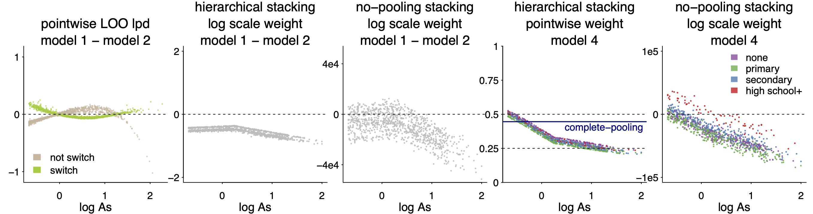
Figure 2: (1) Pointwise difference of leave-one-out log scores between models 1 and 2, plotted against log arsenic. Model 1 poorly fits points with high arsenic. (2) Posterior mean of pointwise unconstrained weight difference between models 1 and 2, $\alpha_{2}(x)-\alpha_{1}(x)$ in hierarchical stacking. (3) Pointwise log weight difference between models 1 and 2 in no-pooling stacking. (4) Posterior mean of $w_{4}(x)$, the weight assigned to model 4, in hierarchical stacking, displayed against log arsenic and education levels. There are few samples with high school education and above, whose effect on model weights is pooled toward the shared mean. The blue line is the complete-pooling stacking. (5) The unconstrained weight of model 4, $\alpha_{4}(x)$, in no-pooling stacking. The “high school” effect stands out and the resulting model weights $\operatorname{\mathbf{w}}$ are nearly all zeroes and ones.

The leftmost panel in Figure 2 displays the pointwise difference of leave-one-out log scores for models 1 and 2 against log arsenic values in training data. Intuitively, model 1 fits poorly for data with high arsenic. In line with this evidence, hierarchical stacking assigns model 1 an overall low weight, and especially low for the right end of the arsenic levels. The second panel shows the pointwise posterior mean of unconstrained weight difference between model 1 and 2, $\alpha_{2}(x)-\alpha_{1}(x)$, against the arsenic values in training data. The no-pooling stacking reveals a similar direction that model 1’s weight should be lower with a higher arsenic value, but for lack of hierarchical prior regularization, the fitted $\alpha_{2}(x)-\alpha_{1}(x)$ is orders of magnitude larger (the third panel). As a result, the realized pointwise weights $\operatorname{\mathbf{w}}$ are nearly either zero or one.

The rightmost two columns in Figure 2 display the fitted pointwise weights of model 4 against log arsenic values and education level in test data. Because only a small proportion (7%) of respondents had high school education and above, the no-pooling stacking weight for this category is largely determined by small sample variation. Hierarchical stacking partially pools this “high school” effect toward the shared posterior mean of all educational levels, and the realized hierarchical stacking model weights do not clearly depend on education levels.

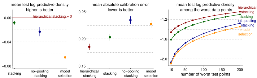
Figure 3: We evaluate hierarchical, complete-pooling and no-pooling stacking, and model selection on three metrics: (a) average log predictive densities on test data, where we set the hierarchical stacking as benchmark 0, (b) calibration error: discrepancy between the predicted positive probability and realized proportion of positives in test data, averaged over 20 equally spaced bins, and (c) average log predictive densities among the $10\leq n_{0}\leq 200$ worst test data points. We repeat 50 random training-test splits with training size 2000 and test size 1020.

We evaluate model fit on the following three metrics. To reduce randomness, we evaluate all these metrics averaging over 50 random training-test splits.

1. The log predictive densities averaged over test data. In the first panel of Figure 3, we set hierarchical stacking as a baseline and all other methods attain lower predictive densities.

2. The $L_{1}$ calibration error. We set 20 equally spaced bins between 0 and 1. For each bin and each learning algorithm, we collect test data points whose model-predicted positive probability falling in that bin, and compute the absolute discrepancy between the realized proportion of positives in test data and the model-predicted probabilities. The middle panel in Figure 3 displays the resulted calibration error averaged over 20 bins. The proposed hierarchical stacking has the lowest error. No-pooling stacking has the highest calibration error despite its higher overall log predictive densities than model selection, suggesting prediction overconfidence.

3. We compute the average log predictive densities of four methods among the $n_{\mathrm{worst}}$ most shocking test data points (the ones with lowest predictive densities conditioning on a given method) for $n_{\mathrm{worst}}$ varying from 10 to 200 and the total test data has size 1020. As exhibited in the last panel in Figure 3, the proposed hierarchical stacking consistently outperforms all other approaches for all $n_{\mathrm{worst}}$: a robust performance in the worst-case scenario.

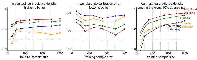
Figure 4: Same comparisons as Figure 3, with training sample size varying from 100 to 1200.

Figure 4 presents the same comparisons of four methods while the training sample size $n_{\mathrm{train}}$ varies from 100 to 1200 (averaged over 50 random training-test splits). In agreement with the heuristic in Figure 1, the most complex method—no-pooling stacking—performs especially poorly with a small sample size. By contrast, the simplest method, model selection, reaches its peak elpd quickly with a moderate sample size but cannot keep improving as training data size grows. The proposed hierarchical stacking performs the best in this setting under all metrics.

5.2 Gaussian process regression weighted by another Gaussian process

The local model averaging (12) tangles a $x$-dependent weight $\operatorname{\mathbf{w}}(x)$ and $x$-dependent individual prediction $p(y|x,M_{k})$. If the individual model $y|x,M_{k}$ is already big enough to have exhausted “all” variability in input $x$, is there still a room for improvement by modeling local model weights $\operatorname{\mathbf{w}}(x)$? The next example suggests a positive answer.

Consider a regression problem with observations $\{y_{i}\}_{i=1}^{n}$ at one-dimensional input locations $\{x_{i}\}_{i=1}^{n}$. To the data we fit a Gaussian process regression on the latent function $f$ with zero mean and squared exponential covariance, and independent noise $\epsilon$:

$$y_{i}=f(x_{i})+\epsilon_{i},~{}\epsilon_{i}\sim\mbox{normal}(0,\sigma),~{}f(x)\sim\mathcal{GP}\left(0,a^{2}\exp\left(-\frac{(x-x^{\prime})^{2}}{\rho^{2}}\right)\right).$$ (25)

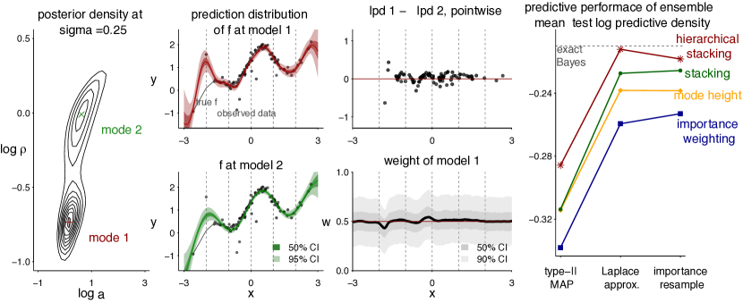
Figure 5: From left to right, Column 1: posterior density at $\sigma=0.25$. At least two modes exist. Column 2: predictive distribution of $y$ from two modes. Column 3: the pointwise companion of log predictive density of the Laplace approximations at two modes, and the hierarchical stacking weight of mode 1. Column 4: the test data mean predictive densities of the weighted model, where individual components in the final model consists of either the MAP, Laplace approximation, or importance sampling around the two modes, and the weighting methods include hierarchical stacking, complete-pooling stacking, mode heights and importance weighing.

We adopt training data from Neal, (1998). They were generated such that the posterior distribution of hyperparameters $\theta=(a,\rho,\sigma)$ contains at least two isolated modes (see the first panel in Figure 5). We consider three mode-based approximate inference of $\theta|y$: (a) Type-II MAP, where we pick the local modes of hyperparameters that maximizes the marginal density $\hat{\theta}=\arg\max p(\theta|y)$, and further draw local variables $f|\hat{\theta},y$, (b) Laplace approximation of $\theta|y$ around the mode, and (c) importance resampling where we draw uniform samples near the mode and keep sample with probability proportional to $p\left(\theta|y\right)$. In the existence of two local modes $\hat{\theta}_{1},\hat{\theta}_{2}$, we either obtain two MAPs or two nearly-nonoverlapped draws, further leading to two predictive distributions. Yao et al., (2020) suggests using complete-pooling stacking to combine two predictions, which shows advantages over other ad-hoc weighting strategies such as mode heights or importance weighting.

Visually, mode 1 has smaller length scale, more wiggling and attracted by training data. Because of a better overall fit, it receives higher complete-stacking weights. However, the wiggling tail makes its extrapolation less robust. We now run hierarchical stacking with $x$-dependent weight $w_{k}(x)$ for mode $k=1,2$ by placing another Gaussian process prior on unconstrained weight logit$(w_{1}(x))$ with squared exponential covariance,

$$w_{1}(x)=\text{invlogit}\left(\alpha(x)\right),~{}~{}\alpha(x)\sim\mathcal{GP}(0,K(x)).$$

Despite using the same GP prior, this is not related to the training regression model (25). To evaluate how good the weighted ensemble is, we generate independent holdout test data $(\tilde{x}_{i},\tilde{y}_{i})$. Both training and test inputs, $x$ and $\tilde{x}$, are distributed from normal$(0,1)$. As presented in the rightmost panel in Figure 5, for all three approximate inferences, hierarchical stacking always has a higher mean test log predictive density than complete pooling stacking and other weighting schemes.

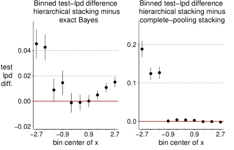
Figure 6: Compare hierarchical stacking with (left) stacking of two Laplace approximations or (right) a long-chain exact Bayes from the true model. We compare the binned test log predictive densities over 10 equally spaced bins on $(-3,3)$. A positive value means hierarchical stacking has a better fit than the counterpart.

In this dataset, exact MCMC is able to explore both posterior modes in model (25) after a long enough sampling. Gaussian process regression equipped with exact Bayesian inference can be regarded as the “always true" model here. Hierarchical stacking achieves a similar average test data fit by combining two Laplace approximations. Furthermore, hierarchical stacking has better predictive performance under covariate shift. To examine local model fit, we generate another independent holdout test data, with results shown in Figure 6. This time the test inputs $\tilde{x}$ are from uniform$(-3,3)$. We divide the test data into 10 equally spaced bins and compute the mean test data log predictive density inside each bin. Compared with exact inference, hierarchical stacking has comparable performance in the bulk region of $x$, while it yields higher predictive densities in the tail, suggesting a more reliable extrapolation.

5.3 U.S. presidential election forecast

We explore the use of hierarchical stacking on a practical example of forecasting polls for the 2016 United States presidential election. Since the polling data are naturally divided into states, it provides a suitable platform for hierarchical stacking in which model weights vary on states.

To create a pool of candidate models, we first concisely describe the model of Heidemanns et al., (2020), an updated dynamic Bayesian forecasting model (Linzer,, 2013) for the presidential election, and then follow up with different variations of it. Let $i$ be the index of an individual poll, $y_{i}$ the number of respondents that support the Democratic candidate, and $n_{i}$ the number of respondents who support either the Democratic or the Republican candidate in the poll. Let $s[i]$ and $t[i]$ denote the state and time of poll $i$ respectively. The model is expressed by

$$y_{i} \sim\text{Binomial}(\theta_{i},n_{i}),$$

$$\theta_{i} =\begin{cases}\text{logit}^{-1}(\mu_{s[i],t[i]}^{b}+\alpha_{i}+\zeta_{i}^{\text{state}}+\xi_{s[i]}),&i\text{ is a state poll,}\\ \text{logit}^{-1}(\sum_{s=1}^{S}u_{s}\mu_{s,t[i]}^{b}+\alpha_{i}+\zeta_{i}^{\text{national}}+\sum_{s=1}^{S}u_{s}\xi_{s}),&i\text{ is a national poll,}\end{cases}$$ (26)

where superscripts denote parameter names, and subscripts their indexes. The term $\mu^{b}$ is the underlying support for the Democratic candidate, and $\alpha_{i}$, $\zeta$, and $\xi$ represent different bias terms. $\alpha_{i}$ is further decomposed into

$$\alpha_{i}=\mu_{p[i]}^{c}+\mu_{r[i]}^{r}+\mu_{m[i]}^{m}+z\epsilon_{t[i]},$$ (27)

where $\mu^{c}$ is the house effect, $\mu^{r}$ polling population effect, $\mu^{m}$ polling mode effect, and $\epsilon$ an adjustment term for non-response bias. Furthermore, an autoregressive (AR(1)) prior is given to the $\mu^{b}$: $\mu_{t}^{b}|\mu_{t-1}^{b}\sim\text{MVN}(\mu_{t-1}^{b},\Sigma^{b}),$ where $\Sigma^{b}$ is the estimated state-covariance matrix and $\mu_{T}^{b}$ is the estimate from the fundamentals.

Although we believe this model reasonably fits data, there is always room for improvement. Our pool of candidates consists of eight models. $M_{1}$: The fundamentals-based model of Abramowitz, (2008). $M_{2}$: The model of Heidemanns et al., (2020). $M_{3}$: $M_{2}$ without the fundamentals prior, $\mu_{T}^{b}=0$. $M_{4}$: $M_{2}$ with an AR(2) structure, $\mu_{t}^{b}|\mu_{t-1}^{b},\mu_{t-2}^{b}\sim\text{MVN}(0.5\mu_{t-1}^{b}\mu_{t-2}^{b},\Sigma^{b})$. $M_{5}$: simplify $M_{2}$ without polling population effect, polling mode effect, and the adjustment trend for non-response bias, $\alpha_{i}=\mu_{p[i]}^{c}$. $M_{6}$: $M_{2}$ where we added an extra regression term $\beta_{\mathrm{stock}}\mathrm{stock}_{t[i]}$ into model (26) using the S&P 500 index at the time of poll $i$. $M_{7}$: $M_{2}$ without the entire shared bias term, $\alpha_{i}=0$. $M_{8}$: $M_{2}$ without hierarchical structure on states.

We equip hierarchical stacking with either the basic independent prior (9) or the state-correlated prior (15). The prior correlation $\Omega$ is estimated using a pool of state-level macro variables (election results in the past, racial makeup, educational attainment, etc.), and has already been used in some of the individual models to partially pool state-level polling. We plug this pre-estimated prior correlation in the correlated stacking prior (15) and refer to it as “hierarchical stacking with correlation" in later comparisons.

Since the data are longitudinal, we evaluate different pooling approaches using a one-week-ahead forecast with an expanding window for each conducted poll. We extract the fitted one-week-ahead predictions from each individual model, and train hierarchical stacking, complete-pooling, and no-pooling stacking, and evaluate the combined models by computing their mean log predictive densities on the unseen data next week. To account for the non-stationarity discussed in Section 2.5, we only use the last four weeks prior to prediction day for training model averaging. In the end we obtain a trajectory of this back-testing performance of hierarchical stacking, complete-pooling stacking, no-pooling stacking, and single model selection.

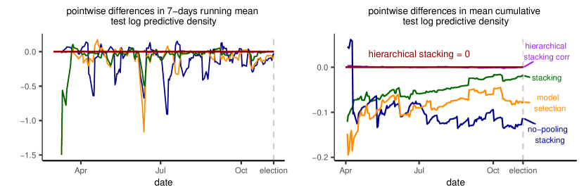
Figure 7: Left: pointwise differences in 7-day running mean log predictive densities on one-week-ahead test data, where we set the hierarchical stacking as benchmark 0. Right: pointwise differences in cumulative average predictive log density by date. The advantage of hierarchical stacking is most noticeable toward the beginning, where there are fewer polls available.

Figure 8: Mean test log predictive densities with 50% and 95% confidence intervals, among subsets of states with few, moderate, and many number of state polls, and among all states. Correlated hierarchical stacking is set as reference 0. It is better than independent hierarchical stacking when data are scarce. Complete-pooling stacking is close to hierarchical stacking in small states but worse in bigger states.

The left-hand side of Figure 7 shows the seven-day running average of the one-week-ahead back-test log predictive density from models combined with various approaches. The right-hand side of Figure 7 shows the overall cumulative one-week-ahead back-test log predictive density. We set the uncorrelated hierarchical stacking to be a constant zero for reference. Hierarchical stacking performs the best, followed by stacking, no-pooling stacking, and model selection respectively. The advantage of hierarchical stacking is highest at the beginning and slowly decreases the closer we get to election day. As we move closer to the election, more polls become available, so the candidate models become better and also more similar since some models only differ in priors. As a result, all combination methods eventually become more similar. No-pooling stacking has high variance and hence performs the worst out of all combination methods. Hierarchical stacking with correlated prior performs similarly to the independent approach, with a minor advantage at the beginning of the year, where the prior correlation stabilizes the state weights where the data are scarce, and later we see this advantage more discernible in individual states.

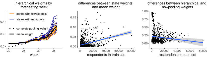
Figure 9: Hierarchical stacking weights for $M_{1}$ in the polling example. Left: weights for $M_{1}$ of the 10 states with fewest polls and with most polls over time. Dotted line shows the complete-pooling stacking weight and the solid black line is the nationwide mean weight. States with fewer polls are shrunken more toward the mean. Middle: absolute differences between state-wise hierarchical stacking weights and the nationwide mean, against number of respondents. The blue line is the linear trend reference. States with smaller sample sizes are more pooled to the mean. Right: absolute differences between hierarchical stacking and no-pooling stacking weights, generally decreasing with bigger sample sizes.

To examine small area estimates, we divided states into three categories based on how many state polls were conducted. Figure 8 shows the overall mean pointwise differences in test log predictive densities divided by these categories, along with a fourth panel over all states. No-pooling stacking performs the worst in all panels. An explanation for that could be that we are using a four-week moving window to tackle non-stationarity, which might not contain enough data for the no-pooling method. The variance of the no-pooling is amended by the hierarchical approach, which performs on par with stacking with scarcer data and outperforms it otherwise. Figure 14 in Appendix E shows the state-level cumulative log predictive density by time. With a large number of state polls available, for example, close to election day in Florida and North Carolina, no-pooling stacking performs well. In states with fewer polls, no-pooling stacking is unstable. Hierarchical stacking alleviates this instability while retaining enough flexibility for a good performance when large data come in.

Figure 9 illustrates how cell size affects the pooling effect. The first panel shows the hierarchical stacking state-wise weights for the first candidate model $w_{1j}$ as a function of date. For either early-date forecasts or states with few polls, hierarchical stacking weights are more pooled toward the shared nationwide mean. The middle and right panels compare the difference between state-wise hierarchical stacking weights and the nationwide mean, or with no-pooling weights, against the total number of respondents for each state and prediction date. The cells with more observed data are less pooled and closer to their no-pooling optimums, and vice versa.

6 Discussion

6.1 Robustness in small areas

The input-varying model averaging is designed to improve both the overall averaged prediction $\operatorname{\mathrm{E}}_{\tilde{y},\tilde{x}}(\log p_{\mathrm{}}(\tilde{y}|\tilde{x}))$ and conditional prediction $\operatorname{\mathrm{E}}_{\tilde{y}|\tilde{x}=x_{0}}(\log p_{\mathrm{}}(\tilde{y}|\tilde{x}))$, whereas these two tasks are subject to a trade-off in complete-pooling stacking.

In addition, the partial pooling prior (9) borrows information from other cells, which stabilizes model weights in small cells where there are not enough data for no-pooling stacking. For a crude mean-field approximation, the likelihood in the discrete model (11) is approximately $\prod_{j,k}\operatorname{\mbox{normal}}(\alpha_{jk}^{\mathrm{mode}},\lambda_{jk})$, where $\alpha^{\mathrm{mode}}=\arg\max_{\alpha}\sum_{i=1}^{n}\log\left(\sum_{k=1}^{K}w_{k}(x_{i})p_{k,-i}\right)$ is the unconstrained no-pooling stacking weight, and $-\lambda_{jk}^{-2}=\frac{\partial^{2}}{\partial\alpha^{2}_{jk}}|_{\mathrm{mode}}\sum_{i=1}^{n}\log\left(\sum_{k=1}^{K}w_{k}(x_{i})p_{k,-i}\right)$ is the diagonal element of the Hessian. Because $\alpha_{jk}$ appears in $n_{j}$ terms of the summation, $\lambda_{jk}=\mathcal{O}(n_{j}^{-{1}/{2}})$ for a given $k$. Combined with the prior $\alpha_{jk}\sim\operatorname{\mbox{normal}}(\mu_{k},\sigma_{k})$, the conditional posterior mean of the $k$-th model weight in the $j$-th cell is the usual precision-weighed average of the no-pooling optimum and the shared mean: $\alpha_{jk}^{\mathrm{post}}\coloneqq\operatorname{\mathrm{E}}(\alpha_{jk}|\lambda_{jk},\sigma_{k},\mu_{k},\mathcal{D})\approx({{\lambda^{-2}_{jk}}\alpha_{jk}^{\mathrm{mode}}+{\sigma_{k}^{-2}}\mu_{k}})({\lambda^{-2}_{jk}}+{\sigma_{k}^{-2}})^{-1}.$ Hence for a given model $k$, $|\alpha_{jk}^{\mathrm{mode}}-\alpha_{jk}^{\mathrm{post}}|=\mathcal{O}({n_{j}^{-1}})$. Larger pooling usually occurs in smaller cells. This pooling factor is in line with Figure 9 and general ideas in hierarchical modeling (Gelman and Pardoe,, 2006). Our full-Bayesian solution also integrates out $\mu_{k}$ and $\sigma_{k}$, which further partially pools across models.

The possibility of partial pooling across cells encourages open-ended data gathering. In the election polling example, even if a pollster is only interested in the forecast of one state, they could gather polling data from everywhere else, fit multiple models, evaluate models on each state, and use hierarchical stacking to construct model averaging, which is especially applicable when the state of interest does not have enough polls to conduct a meaningful model evaluation individually. In this context swing states naturally have more state polls, so that the small-area estimation may not be crucial, but in general, we conjecture that the hierarchical techniques can be useful for model evaluation and averaging in a more general domain adaptation setting. Without going into extra details, hierarchical models are as useful for making inferences from a subset of data (small-area estimation) as to generalize data to a new area (extrapolation). When the latter task is the focus, hierarchical stacking only needs to redefine the leave-one-data-out predictive density (6) by leave-one-cell-out $p_{k,-i}\coloneqq\int_{\Theta_{k}}p(y_{i}|\theta_{k},x_{i},z_{i},M_{k})p\left(\theta_{k}|M_{k},\{(x_{i^{\prime}},z_{i^{\prime}},y_{i^{\prime}}):{x_{i^{\prime}}}\neq x_{i}\}\right)d\theta_{k}.$

6.2 Using hierarchical stacking to understand local model fit

We use hierarchical stacking not only as a tool for optimizing predictions but also as a way to understand problems with fitted models. The fact that hierarchical stacking is being used is already an implicit recognition that we have different models that perform better or worse in different subsets of data, and it can valuable to explore the conditions under which different models are fitting poorly, reveal potential problems in the data or data processing, and point to directions for individual-model improvement.

Vehtari et al., (2017) and Gelman et al., (2020) suggested to examine the pointwise cross-validated log score $\log p_{k,-i}$ as a function of $x_{i}$, and see if there is a pattern or explanation for why some observations are harder to fit than others. For example, the first panel of Figure 2 seems to indicate that Model 1 is incapable of fitting the rightmost 10–15 non-switchers. However, $\log p_{k,-i}$ contains a non-vanishing variance since $y_{i}$ is a single realization from $p_{t}(y|x_{i})$. Despite its merit in exploratory data analysis, it is hard to tell from the raw cross validation scores whether Model 1 is incapable of fitting high arsenic or is merely unlucky for these few points. The hierarchical stacking weight $\operatorname{\mathbf{w}}(x)$ provides a smoothed summary of how each model fits locally in $x$ and comes with built-in Bayesian uncertainty estimation. For example, in Figure 5, $\log p_{1,-i}-\log p_{2,-i}$ has a slightly inflated right tail, but this small bump is smoothed by stacking, and the local weight therein is close to $(0.5,0.5)$.

6.3 Retrieving a formal likelihood from an optimization objective

The implication of hierarchical stacking (11) being a formal Bayesian model is that we can evaluate its posterior distribution as with a regular Bayesian model. For example, we can run (approximate) leave-one-out cross validation of the the stacking posterior $p(\operatorname{\mathbf{w}}|\mathcal{D}_{-i})\propto p(\operatorname{\mathbf{w}}|\mathcal{D})/p(y_{i}|x_{i},\operatorname{\mathbf{w}})=p(\operatorname{\mathbf{w}}|\mathcal{D})/\left(\sum_{k=1}^{K}w_{k}(x_{i})p_{k,-i}\right)$. In practice, we only need to fit the stacking model (11) once, collect a size-$S$ MCMC sample of stacking parameters from the full posterior $p(\operatorname{\mathbf{w}}|\mathcal{D})$, denoted by $\{(w_{k1}(x_{i}),\dots,w_{kS}(x_{i}))\}_{i,k}$, compute the PSIS-stabilized importance ratio of each draw $r_{is}\approx\left(\sum_{k=1}^{K}w_{ks}(x_{i})p_{k,-i}\right)^{-1}$, and then compute the mean leave-one-out cross validated log predictive density to evaluate the overall out-of-sample fit of the final stacked model:

$$\mathrm{elpd}^{\mathrm{loo}}_{\mathrm{stacking}} =\sum_{i=1}^{n}\log\int_{\mathcal{S}_{K}}p(y_{i}|x_{i},\operatorname{\mathbf{w}}(x_{i}))p(\operatorname{\mathbf{w}}(x_{i})|\mathcal{D}_{-i})d(\operatorname{\mathbf{w}}(x_{i}))$$

$$\approx\sum_{i=1}^{n}\log\frac{\sum_{s=1}^{S}\left(r_{is}\sum_{k=1}^{K}w_{ks}(x_{i})p_{k,-i}\right)}{\sum_{s=1}^{S}r_{is}}.$$ (28)

As discussed in Section 4, the same task of out-of-sample prediction evaluation in an optimization-based stacking requires double cross validation (refit the model $n(n-1)$ times if using leave-one-out), but now becomes almost computationally free by post-processing posterior draws of stacking.

The Bayesian justification above applies to log-score stacking. In general, we cannot convert an arbitrary objective function into a log density—its exponential is not necessarily integrable, and, even if it is, the resulted density does not necessarily correspond to a relevant model. Take linear regression for example, the ordinary least square estimate $\arg\min_{\beta}\sum_{i=1}^{n}(y_{i}-x_{i}^{T}\beta)^{2}$ is identical to the maximum likelihood estimate of $\beta$ from a probabilistic model $y_{i}|x_{i},\beta,\sigma\sim\operatorname{\mbox{normal}}(x_{i}^{T}\beta,\sigma)$ with flat priors. But the directly adapted “log posterior density" from the negative $L^{2}$ loss, $\log p(\beta|y)=-\sum_{i=1}^{n}(y_{i}-x_{i}^{T}\beta)^{2}+C$, differs from the Bayesian inference of the latter probabilistic model unless $\sigma\equiv 1$. The hierarchical stacking framework may still apply to other scoring rules, while we leave their Bayesian calibration for future research.

6.4 Statistical workflow for black box algorithms

Unlike our previous work (Yao et al.,, 2018) that merely applied stacking to Bayesian models, the present paper converts optimization-based stacking itself into a formal Bayesian model, analogous to reformulating a least-squares estimate into a normal-error regression. Breiman, (2001) distinguished between two cultures in statistics: the generative modeling culture assumes that data come from a given stochastic model, whereas the algorithmic modeling treats the data mechanism unknown and advocates black box learning for the goal of predictive accuracy. As a method that Breiman himself introduced (along with Wolpert,, 1992), stacking is arguably closer to the algorithmic end of the spectrum, while our hierarchical Bayesian formulation pulls it toward the generative modeling end.

Such a full-Bayesian formulation is appealing for two reasons. First, the generative modeling language facilitates flexible data inclusion during model averaging. For example, the election forecast model contains various outcomes on state polls and national polls from several pollsters, and pollster-, state- and national-level fundamental predictors, and prior state-level correlations. It is not clear how methods like bagging or boosting can include all of them. Data do not have to conveniently arrive in independent $(x_{i},y_{i})$ pairs and compliantly await an algorithm to train upon. Second, instead of a static algorithm, hierarchical stacking is now part of a statistical workflow (Gelman et al.,, 2020). It then enjoys all the flexibility of Bayesian model building, fitting, and checking—we can incorporate other Bayesian shrinkage priors as add-on components without reinventing them; we can run a posterior predictive check or approximate leave-one-out cross validation (6.3) to assess the out-of-sample performance of the final stacking model; we may even further select, stack, or hierarchically stack a sequence of hierarchical stacking model with various priors and parametric forms. Looking ahead, the success of this work encourages more use of generative Bayesian modeling to improve other black box prediction algorithms.

Acknowledgements

The authors would like to thank the National Science Foundation, Institute of Education Sciences, Office of Naval Research, National Institutes of Health, Sloan Foundation, and Schmidt Futures for partial financial support. Gregor Pirš is supported by the Slovenian Research Agency Young researcher grant.

Appendix

Appendix A A theoretical example

Before theorem proofs, we first consider a toy example. It can be solved with a closed form solution and illustrates how Theorems 1–4 apply.

As shown in Figure 10, the true data generating process (DG) of the outcome is $y\sim\mathrm{uniform}(-3,1)$, and there are two given (pre-trained) models with spike-and-slab predictive distributions

$$M_{1}:y\sim.99~{}\mathrm{uniform}(-4,0)+.01~{}\mathrm{uniform}(0,2),$$

$$M_{2}:y\sim.99~{}\mathrm{uniform}(0,2)+.01~{}\mathrm{uniform}(-4,0),$$

which yield piece-wise constant predictive densities

$$p_{1}(y)=0.99/4\mathbbm{1}(y\in[-4,0])+0.01/2\mathbbm{1}(y\in[0,2]),$$

$$p_{2}(y)=0.99/2\mathbbm{1}(y\in[0,2])+0.01/4\mathbbm{1}(y\in[-4,0]).$$

Using our notation in Section 3.2, the region in which $M_{1}$ predominates is $\mathcal{J}_{1}=[-4,0]$, and $M_{2}$ outperforms on $\mathcal{J}_{2}=(0,2]$ (the conventions send the tie $\{0\}$ to $M_{1}$). We count their masses with respect to the true DG: $\Pr(\mathcal{J}_{1})=3/4$ and $\Pr(\mathcal{J}_{2})=1/4$.

Complete-pooling stacking solves

$$\max_{\operatorname{\mathbf{w}}\in\mathcal{S}_{2}}\int_{-3}^{1}1/4\log\Bigl{(} (w_{1}0.99/4+w_{2}0.01/4)\mathbbm{1}(y\in[-4,0])+$$

$$(w_{2}0.99/2+w_{1}0.01/2)\mathbbm{1}(y\in[0,2])\Bigr{)}dy.$$

The exact optimal weight is $w_{1}=0.755$, close to the mass $\Pr(\mathcal{J}_{1})=0.75$ and is irrelevant to the height of each regions. For instance, if the right bump in $M_{2}$ shrinks to the interval $(0,1)$ (i.e., $y\sim 0.99~{}\mathrm{uniform}(0,1)+0.01~{}\mathrm{uniform}(-4,0)$), then the winning margin therein is twice as big, while the winning probability as well as the stacking weight remains nearly unchanged.

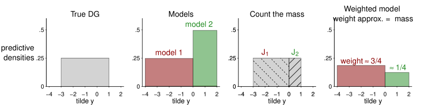
Figure 10: The true data is generated from $\mbox{uniform}(-3,1)$ and there are two models with spikes and slabs on intervals $(-4,0)$ and $(0,2)$ respectively. $\mathcal{J}_{1}$ and $\mathcal{J}_{2}$ in Theorem 1 are $[-4,0]$ and $(0,2]$, with DG probabilities 3/4 and 1/4. The stacking weights are approximately these two probabilities, and irrelevant to how high the winning margins are.

At the pointwise level, stacking behaves as a plurality voting system: as long a model “wins" a sub-region (subject to a prefixed threshold $L$ in condition (19)), the winner take all and its winning margin no longer matters.

By contrast, likelihood-based model averaging techniques such as Bayesian model averaging (BMA, Hoeting et al.,, 1999) and pseudo-Bayesian model averaging (Yao et al.,, 2018) are analogies of proportional representation: every count of the winning margin matters. For illustration, we vary the slab probability $\delta$ in Model 1 and 2:

$$M_{1}\mid\delta:~{}~{}y\sim(1-\delta)\times\mathrm{uniform}(-4,0)+\delta\times\mathrm{uniform}(0,2),$$

$$M_{2}\mid\delta:~{}~{}y\sim(1-\delta)\times\mathrm{uniform}(0,2)+\delta\times\mathrm{uniform}(-4,0).$$

The left column in Figure 11 visualizes the predictive densities from these two models at $\delta=0.2$, $0.33$, and $0.45$.

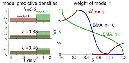
Figure 11: Left: Pointwise predictive density $p(\tilde{y}|M_{1}~{}\mathrm{or}~{}M_{2})$ when the slab probability $\delta$ is chosen 0.2, 1/3 and 0.45. Right: Weight of model 1 in complete-pooling stacking (not defined at $\delta=0.5$) and pseudo-BMA (sample size $n$=1 or 10, not defined at $\delta=0$ or 1) as a function of the slab probability $\delta$. They evolve in the opposite direction. Besides, stacking weights are more polarized when models are more similar.

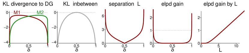
Figure 12: From left: (1) KL divergence between model 1 or model 2 and data generating process. (2) KL divergence between model 1 and model 2. (3) Separation constant $L$. (4) Stacking elpd gain compared with the best individual model. (5) Stacking elpd gain as a function of $L$.

When the slab probability $\delta$ increases from 0 to 0.5, these two models are closer and closer to each other, measured by a smaller KL($M_{1},M_{2}$). The $(0.5,1)$ counterpart is similar, though not exactly symmetric. We compute stacking weight and the expected pseudo-BMA weight with sample size $n$: $w_{1}^{\mathrm{BMA}}(n,\delta)=\left(1+\exp\left(n\operatorname{\mathrm{E}}_{y|\delta}\log p_{2}(y)-n\operatorname{\mathrm{E}}_{y|\delta}\log p_{1}(y)\right)\right)^{-1}$.

Interestingly, pseudo-BMA weight $w_{1}^{\mathrm{BMA}}(n,\delta)$ is strictly decreasing as a function of $\delta\in(0,1)$. This is because when $\delta\to 0^{+}$, log predictive density of model 2 in the left part $\log(\delta/4)\to\infty$ can be arbitrarily small, and the influence of this bad region dominates the overall performance of model 2. By contrast, stacking weight is monotonic non-increasing on $(0,0.5)$ (strictly decreasing on $(0,1/3)$, and remains flat afterwards)—the opposite direction of BMA. Stacking simply recognizes model 1 winning the $[-3,0]$ interval and does not haggle over how much it wins.

In addition, when $\delta=1/3$, $M_{1}$ becomes a uniform density on $[-4,2]$. When $\delta\in(1/3,1/2)$, model 2 is not only strictly worse than model 1 but also provides no extra information for model averaging. Hence stacking assigns it weight zero.

The first two panels in Figure 12 show the KL divergence from model 1 or from model 2 to the data generating process and the KL divergence between model 1 and model 2. The third panel is the largest separation constant $L$ for which the separation condition (19) holds. The last two panels show the stacking epld gain (compared with the best individual model) as a function of $\delta$ and $L$. This constructive example reflects the worst case for it matches the theoretical lower bound $g^{*}(L,K,\rho,\epsilon)=\log(\rho)+(1-\rho)(\log(1-\rho)-\log(K-1))$ (here $L=L,K=2,\rho=1/4,\epsilon=0$) in Theorem 3.

When $\delta\in[1/3,1/2)$, Model 2 still wins on the interval $\mathcal{J}_{2}=(0,2]$ with the separation constant $\epsilon=0$ and $L\leq\log 2$ (the winning margin is maximized at $\delta=1/3$). Nevertheless, a zero stacking weight and a non-zero winning area do not contradict Theorem 1. Indeed, Theorem 2 precisely bounds the mass of the winning region when stacking weight is zero. We provide self-contained theorem proofs in the next section.

Loosely speaking, BMA computes the probability of a model being true (if one model has to be true), while stacking (through the approximation Pr$(\mathcal{J}_{k})$) computes the probability of a model being the best.

Appendix B Proofs of theorems

For briefly, in later proofs we will use the abbreviation for the posterior pointwise conditional predictive density from the $k$-th model:

$$p_{k}(\tilde{y}|\tilde{x})\coloneqq p(\tilde{y}|\tilde{x},M_{k})=\int p(\tilde{y}|\tilde{x},\theta_{k})p(\theta_{k}|\mathcal{D})d\theta_{k},\quad k=1,\dots,K.$$

This subscript index $k$ should not be confused with the notation $t$ as in $p_{t}(\tilde{y}|\tilde{x})$ or $p_{t}(\tilde{y},\tilde{x})$: the unknown conditional or joint density of the true data generating process. The subscript letter ${t}$ is always reserved for “true".

Recall that in this section $\operatorname{\mathbf{w}}^{\mathrm{stacking}}$ refers to the complete-pooling stacking in the population:

$$\operatorname{\mathbf{w}}^{\mathrm{stacking}} \coloneqq\arg\max_{\operatorname{\mathbf{w}}\in\mathcal{S_{K}}}\mathrm{elpd}(\operatorname{\mathbf{w}}),$$

$$\mathrm{elpd}(\operatorname{\mathbf{w}}) =\int_{\mathcal{X}\times\mathcal{Y}}\log\left(\sum_{k=1}^{K}w_{k}p(\tilde{y}|M_{k},\tilde{x})\right)p_{t}(\tilde{y},\tilde{x})d\tilde{y}d\tilde{x}.$$

Theorem 1.

We call $K$ predictive densities $\{p(\tilde{y}=\cdot|\tilde{x}=\cdot,M_{k})\}_{k=1}^{K}$ to be locally separable with a constant pair $L>0$ and $0<\epsilon<1$ with respect to the true data generating process $p_{t}(\tilde{y},\tilde{x})$, if

$$\sum_{k=1}^{K}\int_{(\tilde{x},\tilde{y})\in\mathcal{J}_{k}}\mathbbm{1}\Big{(}\log p(\tilde{y}|\tilde{x},M_{k})<\log p(\tilde{y}|\tilde{x},M_{k^{\prime}})+L,\;\forall k^{\prime}\neq k\Big{)}p_{t}(\tilde{y},\tilde{x})d\tilde{y}d\tilde{x}\leq\epsilon.$$

For a small $\epsilon$ and a large $L$, the stacking weights that solve (3) is approximately the proportion of the model being the locally best model:

$$\operatorname{\mathbf{w}}^{\mathrm{stacking}}_{k}\approx\operatorname{\mathbf{w}}^{\mathrm{approx}}_{k}\coloneqq\Pr(\mathcal{J}_{k})=\int_{\mathcal{J}_{k}}p_{t}(\tilde{y}|\tilde{x})p(\tilde{x})d\tilde{y}d\tilde{x}.$$

in the sense that the objective function is nearly optimal:

$$|\mathrm{elpd}(\operatorname{\mathbf{w}}^{\mathrm{approx}})-\mathrm{elpd}(\operatorname{\mathbf{w}}^{\mathrm{stacking}})|\leq\mathcal{O}(\epsilon+\exp(-L)).$$

Proof.

The expected log predictive density of the weighted prediction $\sum_{k}w_{k}p_{k}(\cdot|x)$ (as a function of $\operatorname{\mathbf{w}}$) is

$$\mathrm{elpd}(\operatorname{\mathbf{w}}) =\int_{\mathcal{X}\times\mathcal{Y}}\log\left(\sum_{l=1}^{K}w_{l}p_{l}(\tilde{y}|\tilde{x})\right)p_{t}(\tilde{y}|\tilde{x})p(\tilde{x})d\tilde{x}d\tilde{y}$$

$$=\sum_{k=1}^{K}\int_{\mathcal{J}_{k}}\log\left(\sum_{l=1}^{K}w_{l}p_{l}(\tilde{y}|\tilde{x})\right)p_{t}(\tilde{y}|\tilde{x})p(\tilde{x})d\tilde{x}d\tilde{y}$$

$$=\sum_{k=1}^{K}\int_{\mathcal{J}_{k}}\log\left(w_{k}p_{k}(\tilde{y}|\tilde{x})+\sum_{l\neq k}w_{l}p_{l}(\tilde{y}|\tilde{x})\right)p_{t}(\tilde{y}|\tilde{x})p(\tilde{x})d\tilde{x}d\tilde{y}$$

$$=\sum_{k=1}^{K}\int_{\mathcal{J}_{k}}\left(\log\left(w_{k}p_{k}(\tilde{y}|\tilde{x})\right)+\log\left(1+\sum_{l\neq k}\frac{w_{l}p_{l}(\tilde{y}|\tilde{x})}{w_{k}p_{k}(\tilde{y}|\tilde{x})}\right)\right)p_{t}(\tilde{y}|\tilde{x})p(\tilde{x})d\tilde{x}d\tilde{y}.$$

The expression is legit for any simplex vector $\operatorname{\mathbf{w}}\in\mathcal{S}_{K}$ that does not contain zeros. We will treat zeros later. For now we only consider a dense weight: $\{\operatorname{\mathbf{w}}\in\mathcal{S}_{K}:w_{k}>0,k=1,\dots K\}$.

Consider a surrogate objective function (the first term in the integral above):

$$\mathrm{elpd}^{\mathrm{surrogate}}(\operatorname{\mathbf{w}}) =\sum_{k=1}^{K}\int_{\mathcal{J}_{k}}\log\left(w_{k}p_{k}(\tilde{y}|\tilde{x})\right)p_{t}(\tilde{y}|\tilde{x})p(\tilde{x})d\tilde{x}d\tilde{y}$$

$$=\sum_{k=1}^{K}\int_{\mathcal{J}_{k}}\left(\log w_{k}+\log p_{k}(\tilde{y}|\tilde{x})\right)p_{t}(\tilde{y}|\tilde{x})p(\tilde{x})d\tilde{x}d\tilde{y}$$

$$=\sum_{k=1}^{K}\log w_{k}\int_{\mathcal{J}_{k}}p_{t}(\tilde{y}|\tilde{x})p(\tilde{x})d\tilde{x}d\tilde{y}+\sum_{k=1}^{K}\int_{\mathcal{J}_{k}}\log p_{k}(\tilde{y}|\tilde{x})p_{t}(\tilde{y}|\tilde{x})p(\tilde{x})d\tilde{x}d\tilde{y}$$

$$=\sum_{k=1}^{K}\left(\Pr(\mathcal{J}_{k})\log w_{k}\right)+\mathrm{constant}.$$

Ignoring the constant term above (the expected cross-entropy between each conditional prediction and the true DG), to maximize the surrogate objective function is equivalent to maximizing $\sum_{k=1}^{K}\Pr(\mathcal{J}_{k})\log w_{k}$, we call this function elbo$(\operatorname{\mathbf{w}})$, the evidence lower bound. To optimize $\mathrm{elpd}^{\mathrm{surrogate}}$ is equivalent to optimizing elbo. We show that this elbo function has a closed form optimum. Using Jensen’s inequality,

$$\mathrm{elbo}(\operatorname{\mathbf{w}}) =\sum_{k=1}^{K}\Pr(\mathcal{J}_{k})\log w_{k}$$

$$=\sum_{k=1}^{K}\Pr(\mathcal{J}_{k})\log\frac{w_{k}}{\Pr(\mathcal{J}_{k})}+\sum_{k=1}^{K}\Pr(\mathcal{J}_{k})\log{\Pr(\mathcal{J}_{k})}$$

$$\leq\log\left(\sum_{k=1}^{K}\Pr(\mathcal{J}_{k})\frac{w_{k}}{\Pr(\mathcal{J}_{k})}\right)+\sum_{k=1}^{K}\Pr(\mathcal{J}_{k})\log{\Pr(\mathcal{J}_{k})}$$

$$=\sum_{k=1}^{K}\Pr(\mathcal{J}_{k})\log{\Pr(\mathcal{J}_{k})}.$$

The equality is attained at $w_{k}=\Pr(\mathcal{J}_{k}),~{}k=1,\dots,K$, which reaches our definition of $\operatorname{\mathbf{w}}^{\mathrm{approx}}$ in Theorem 1.

What remains to be proved is that the surrogate objective function is close to the actual objective. We divide each set $\mathcal{J}_{k}$ into two disjoint subsets $\mathcal{J}_{k}=\mathcal{J}_{\circ}\cup\mathcal{J}_{k}^{\bullet}$, for

$$\mathcal{J}_{k}^{\circ}\coloneqq\left\{(\tilde{x},\tilde{y})\in\mathcal{J}_{k}:\log p(\tilde{y}|\tilde{x},M_{k})<\log p(\tilde{y}|\tilde{x},M_{k^{\prime}})+L\right\};$$

$$\mathcal{J}_{k}^{\bullet}\coloneqq\left\{(\tilde{x},\tilde{y})\in\mathcal{J}_{k}:\log p(\tilde{y}|\tilde{x},M_{k})\geq\log p(\tilde{y}|\tilde{x},M_{k^{\prime}})+L\right\}.$$

The separation condition ensures $\sum_{k=1}^{K}\Pr(\mathcal{J}_{k}^{\circ})\leq\epsilon$.

Let $\Delta(\operatorname{\mathbf{w}})=\mathrm{elpd}(\operatorname{\mathbf{w}})-\mathrm{elpd}^{\mathrm{surrogate}}(\operatorname{\mathbf{w}})$. For any fixed simplex vector $\operatorname{\mathbf{w}}$, this absolute difference of the objective function is bounded by

$$|\Delta(\operatorname{\mathbf{w}})| =\left|\sum_{k=1}^{K}\int_{\mathcal{J}_{k}}\left(\log\left(1+\sum_{l\neq k}\frac{w_{l}p_{l}(\tilde{y}|\tilde{x})}{w_{k}p_{k}(\tilde{y}|\tilde{x})}\right)\right)p_{t}(\tilde{y}|\tilde{x})p(\tilde{x})d\tilde{x}d\tilde{y}\right|$$

$$\leq\sum_{k=1}^{K}\int_{\mathcal{J}_{k}}\left|\log\left(1+\sum_{l\neq k}\frac{w_{l}p_{l}(\tilde{y}|\tilde{x})}{w_{k}p_{k}(\tilde{y}|\tilde{x})}\right)\right|p_{t}(\tilde{y}|\tilde{x})p(\tilde{x})d\tilde{x}d\tilde{y}$$

$$=\sum_{k=1}^{K}\left(\int_{\mathcal{J}_{k}^{\circ}}+\int_{\mathcal{J}_{k}^{\bullet}}\right)\left|\log\left(1+\sum_{l\neq k}\frac{w_{l}p_{l}(\tilde{y}|\tilde{x})}{w_{k}p_{k}(\tilde{y}|\tilde{x})}\right)\right|p_{t}(\tilde{y}|\tilde{x})p(\tilde{x})d\tilde{x}d\tilde{y}$$

$$\leq\sum_{k=1}^{K}\int_{\mathcal{J}_{k}^{\circ}}\log(1+\sum_{l\neq k}\frac{w_{l}}{w_{k}})p_{t}(\tilde{y}|\tilde{x})p(\tilde{x})d\tilde{x}d\tilde{y}+\sum_{k=1}^{K}\int_{\mathcal{J}_{k}^{\bullet}}\sum_{l\neq k}\frac{w_{l}}{w_{k}}\frac{p_{l}(\tilde{y}|\tilde{x})}{p_{k}(\tilde{y}|\tilde{x})}p_{t}(\tilde{y}|\tilde{x})p(\tilde{x})d\tilde{x}d\tilde{y}$$

$$\leq\left(\sum_{k=1}^{K}\sum_{l\neq k}\frac{w_{l}}{w_{k}}\right)\left(\sum_{k=1}^{K}\int_{\mathcal{J}_{k}^{\circ}}p_{t}(\tilde{y}|\tilde{x})p(\tilde{x})d\tilde{x}d\tilde{y}+\sum_{k=1}^{K}\int_{\mathcal{J}_{k}^{\bullet}}\frac{p_{l}(\tilde{y}|\tilde{x})}{p_{k}(\tilde{y}|\tilde{x})}p_{t}(\tilde{y}|\tilde{x})p(\tilde{x})d\tilde{x}d\tilde{y}\right)$$

$$\leq\left(\sum_{k=1}^{K}\frac{1-w_{k}}{w_{k}}\right)(\epsilon+\exp(-L)).$$

The second inequality used $\log(1+x)\leq x$ for $x\geq 0$.

The exact optima of objective function is $\operatorname{\mathbf{w}}^{\mathrm{stacking}}$. Using the inequality above twice,

$$0\leq\mathrm{elpd}(\operatorname{\mathbf{w}}^{\mathrm{stacking}})-\mathrm{elpd}(\operatorname{\mathbf{w}}^{\mathrm{approx}}) \leq|\mathrm{elpd}^{\mathrm{surrogate}}(\operatorname{\mathbf{w}}^{\mathrm{stacking}})-\mathrm{elpd}(\operatorname{\mathbf{w}}^{\mathrm{stacking}})|$$

$$\qquad+|\mathrm{elpd}^{\mathrm{surrogate}}(\operatorname{\mathbf{w}}^{\mathrm{approx}})-\mathrm{elpd}(\operatorname{\mathbf{w}}^{\mathrm{approx}})|$$

$$\qquad+\mathrm{elpd}^{\mathrm{surrogate}}(\operatorname{\mathbf{w}}^{\mathrm{stacking}})-\mathrm{elpd}^{\mathrm{surrogate}}(\operatorname{\mathbf{w}}^{\mathrm{approx}})$$

$$\leq|\Delta(\operatorname{\mathbf{w}}^{\mathrm{approx}})|+|\Delta(\operatorname{\mathbf{w}}^{\mathrm{stacking}})|$$

$$\leq\sum_{k=1}^{K}\left(\frac{1-w_{k}^{\mathrm{approx}}}{w_{k}^{\mathrm{approx}}}+\frac{1-w_{k}^{\mathrm{stacking}}}{w_{k}^{\mathrm{stacking}}}\right)(\epsilon+\exp(-L)).$$

It has almost finished the proof except for the simplex edge where $w_{k}^{\mathrm{stacking}}$ or $w_{k}^{\mathrm{approx}}$ attains zero.

Without loss of generality, if $w_{1}^{\mathrm{approx}}=0,w_{k}^{\mathrm{approx}}\neq 0,\forall k\neq 1$, which means $p(\tilde{y}|M_{k},\tilde{x})$ is always inferior to some other models. This will only happen if $p(\tilde{y}|M_{k},\tilde{x})$ is almost sure zero (w.r.t $p_{t}(\tilde{y}|\tilde{x})p(\tilde{x})$) hence we can remove model 1 from the model list, and the same $\mathcal{O}(\epsilon+\exp(-L))$ bound applies to remaining model $2,\dots,K$. If there are more than one zeros, repeat until all zeros have been removed.

Next, we deal with $w_{1}^{\mathrm{stacking}}=0,w_{k}^{\mathrm{stacking}}\neq 0,\forall k\neq 1$. If $w_{1}^{\mathrm{approx}}=0$, too, then we have solved in the previous paragraph. If not, Theorem 2 shows that $w_{1}^{\mathrm{approx}}$ has to be a small order term:

$$\Pr(\mathcal{J}_{1})\leq(1+(\exp(L)-1)(1-\epsilon)+\epsilon)^{-1}<\exp(-L)+\epsilon.$$

We leave the proof of this inequality in Theorem 2.

The contribution of the first model in the surrogate model is at most $\Pr(\mathcal{J}_{1})\log\Pr(\mathcal{J}_{1})$. After we remove the first model from the model list, with the surrogate model elpd changes by at most a small order term, not affecting the final bound. Because the separation condition with constant $(\epsilon,L)$ applies to model $1,\dots,K$, and due to lack of a competition source, the same separation condition applies to model $2,\dots,K$ and the same bound applies.

∎

Theorem 2.

When the separation condition (19) holds, and if the $k$-th model has zero weight in stacking, $w_{k}^{\mathrm{stacking}}=0$, then the probability of its winning region is bounded by:

$$\Pr(\mathcal{J}_{k})\leq\left(1+(\exp(L)-1)(1-\epsilon)+\epsilon\right)^{-1}.$$

The right hand side can be further upper-bounded by $\exp(-L)+\epsilon$.

Proof.

Without loss of generality, assume $w_{1}^{\mathrm{stacking}}=0$. Let $p_{0}(\tilde{y}|\tilde{x})=\sum_{k=2}^{K}\operatorname{\mathbf{w}}^{\mathrm{stacking}}{p_{k}(\tilde{y}|\tilde{x})}$. Consider a constrained objective $\widetilde{\mathrm{elpd}}(w_{1})=\operatorname{\mathrm{E}}(\log(w_{1}p_{1}(\tilde{y}|\tilde{x})+(1-w_{1})p_{0}(\tilde{y}|\tilde{x})))$ where the expectation is over both $\tilde{y}$ and $\tilde{x}$ as before. Because the max is attained at $w_{1}=0$ and because $\log(\cdot)$ is a concave function, the derivative at any $w_{1}\in[0,1]$ is

$$\frac{d}{dw_{1}}\widetilde{\mathrm{elpd}}(w_{1})=\operatorname{\mathrm{E}}_{\tilde{y},\tilde{x}}\left(\frac{p_{1}(\tilde{y}|\tilde{x})-p_{0}(\tilde{y}|\tilde{x})}{w_{1}p_{1}(\tilde{y}|\tilde{x})+(1-w_{1})p_{0}(\tilde{y}|\tilde{x})}\right)\leq 0.$$

That is

$$0\geq \operatorname{\mathrm{E}}\left(\frac{p_{1}(\tilde{y}|\tilde{x})-p_{0}(\tilde{y}|\tilde{x})}{p_{0}(\tilde{y}|\tilde{x})}\right)$$

$$= \Pr(\mathcal{J}_{1})\operatorname{\mathrm{E}}[\frac{p_{1}(\tilde{y}|\tilde{x})-p_{0}(\tilde{y}|\tilde{x})}{p_{0}(\tilde{y}|\tilde{x})}|\mathcal{J}_{1}]+(1-\Pr(\mathcal{J}_{1}))\operatorname{\mathrm{E}}[\frac{p_{1}(\tilde{y}|\tilde{x})-p_{0}(\tilde{y}|\tilde{x})}{p_{0}(\tilde{y}|\tilde{x})}|\mathcal{J}_{0}]$$

$$\geq \Pr(\mathcal{J}_{1})\operatorname{\mathrm{E}}[\frac{p_{1}(\tilde{y}|\tilde{x})-p_{0}(\tilde{y}|\tilde{x})}{p_{0}(\tilde{y}|\tilde{x})}|\mathcal{J}_{1}]-(1-\Pr(\mathcal{J}_{1})).$$

Rearranging this inequality arrives at

$$1\geq \Pr(\mathcal{J}_{1})\left(1+\operatorname{\mathrm{E}}[\frac{p_{1}(\tilde{y}|\tilde{x})-p_{0}(\tilde{y}|\tilde{x})}{p_{0}(\tilde{y}|\tilde{x})}|\mathcal{J}_{1}]\right)$$

$$\geq \Pr(\mathcal{J}_{1})(1+(\exp(L)-1)(1-\epsilon)+\epsilon).$$

As a result, the model that has stacking weight zero cannot have a large probability to predominate all other models,

$$\Pr(\mathcal{J}_{1})\leq(1+(\exp(L)-1)(1-\epsilon)+\epsilon)^{-1}<\exp(-L)+\epsilon.$$

∎

Theorem 3.

Let $\rho=\sup_{1\leq k\leq K}\Pr(\mathcal{J}_{k})$, and two deterministic functions $g$ and $g^{*}$ by

$$g(L,K,\rho,\epsilon)=L(1-\rho)(1-\epsilon)-\log K$$

$$\leq g^{*}(L,K,\rho,\epsilon)=L(1-\rho)(1-\epsilon)+\rho\log(\rho)+(1-\rho)(\log(1-\rho)-\log(K-1)).$$

Assuming the separation condition (19) holds for all $k=1,\dots,K$, then the utility gain of stacking is further lower-bounded by

$$\mathrm{elpd}_{\mathrm{stacking}}-\mathrm{elpd}_{k}\geq\max\left(g^{*}(L,K,\rho)+\mathcal{O}(\exp(-L)+\epsilon),0\right).$$

Proof.

As before, we consider the approximate weights: $w_{k}^{\mathrm{approx}}=\Pr(\mathcal{J}_{k})$, and the surrogate elpd $\mathrm{elpd}^{\mathrm{surrogate}}(\operatorname{\mathbf{w}})=\sum_{k=1}^{K}\int_{\mathcal{J}_{k}}\log\left(w_{k}p_{k}(\tilde{y}|\tilde{x})\right)p_{t}(\tilde{y}|\tilde{x})p(\tilde{x})d\tilde{x}d\tilde{y}.$

$$\mathrm{elpd}^{\mathrm{surrogate}}(\operatorname{\mathbf{w}}^{\mathrm{approx}})-\mathrm{elpd}_{k}$$

$$= \sum_{l=1}^{K}\int_{\mathcal{J}_{l}}\log\left(\Pr({\mathcal{J}_{l}})p_{l}(\tilde{y}|\tilde{x})\right)p_{t}(\tilde{y}|\tilde{x})p(\tilde{x})d\tilde{x}d\tilde{y}-\sum_{l=1}^{K}\int_{\mathcal{J}_{l}}\log\left(p_{k}(\tilde{y}|\tilde{x})\right)p_{t}(\tilde{y}|\tilde{x})p(\tilde{x})d\tilde{x}d\tilde{y}$$

$$= \sum_{l=1}^{K}\int_{\mathcal{J}_{l}}\left(\log\Pr({\mathcal{J}_{l}})+\log p_{l}(\tilde{y}|\tilde{x})-\log p_{k}(\tilde{y}|\tilde{x})\right)p_{t}(\tilde{y}|\tilde{x})p(\tilde{x})d\tilde{x}d\tilde{y}$$

$$= \sum_{l=1}^{K}\Pr({\mathcal{J}_{l}})\log\Pr({\mathcal{J}_{l}})+\sum_{l=1}^{K}\mathbbm{1}(l\neq k)\int_{\mathcal{J}_{l}}\log(p_{l}(\tilde{y}|\tilde{x})-\log p_{k}(\tilde{y}|\tilde{x}))p_{t}(\tilde{y}|\tilde{x})p(\tilde{x})d\tilde{x}d\tilde{y}$$

$$= \sum_{l=1}^{K}\Pr({\mathcal{J}_{l}})\log\Pr({\mathcal{J}_{l}})+\sum_{l=1}^{K}\mathbbm{1}(l\neq k)\left(\int_{\mathcal{J}_{l}^{\circ}}+\int_{\mathcal{J}_{l}^{\bullet}}\right)\log(p_{l}(\tilde{y}|\tilde{x})-\log p_{k}(\tilde{y}|\tilde{x}))p_{t}(\tilde{y}|\tilde{x})p(\tilde{x})d\tilde{x}d\tilde{y}$$

$$\geq \sum_{l=1}^{K}\Pr({\mathcal{J}_{l}})\log\Pr({\mathcal{J}_{l}})+(1-\epsilon)(1-\rho)L-\epsilon$$

$$\geq \rho\log\rho+(1-\rho)\log\frac{1-\rho}{K-1}+(1-\epsilon)(1-\rho)L-\epsilon$$

$$= g^{*}(L,K,\rho,\epsilon)-\epsilon.$$

The last inequality comes from the fact that, under the constraint of $\max_{k}\Pr({\mathcal{J}_{k}})=\rho$, the entropy $\sum_{k=1}^{K}\Pr({\mathcal{J}_{k}})\log\Pr({\mathcal{J}_{k}})$ attains its minimal when each of the $\Pr({\mathcal{J}_{k}})$ term equals $(1-\rho)/(K-1)$ except for the largest term $\rho$. This inequality is due to the convexity of $x\log x$.

Finally, using the proof of Theorem 1, the error from the surrogate is bounded,

$$|\mathrm{elpd}^{\mathrm{surrogate}}(\operatorname{\mathbf{w}}^{\mathrm{approx}})-\mathrm{elpd}^{\mathrm{stacking}}(\operatorname{\mathbf{w}}^{\mathrm{stacking}})|\leq\mathcal{O}(\exp(-L)+\epsilon).$$

Hence the overall utility is bounded,

$$\mathrm{elpd}_{\mathrm{stacking}}-\mathrm{elpd}_{k}$$

$$=\left(\mathrm{elpd}_{\mathrm{stacking}}-\mathrm{elpd}^{\mathrm{surrogate}}(\operatorname{\mathbf{w}}^{\mathrm{approx}})\right)+\left(\mathrm{elpd}^{\mathrm{surrogate}}(\operatorname{\mathbf{w}}^{\mathrm{approx}})-\mathrm{elpd}_{k}\right)$$

$$\geq g^{*}(L,K,\rho)+\mathcal{O}(\exp(-L)+\epsilon).$$

Because selection is always a specials case of averaging, the utility is further bounded below by 0.

To replace $g^{*}(\cdot)$ with the looser bound $g(\cdot)$, we only need to ensure $\rho\log\rho+(1-\rho)\log\frac{1-\rho}{K-1}\geq-\log K$, for the range $\rho\in[1/K,1),K\geq 2$. The proof is elementary. For any fixed $K\geq 2$, let $h(\rho)=\rho\log\rho+(1-\rho)\log\frac{1-\rho}{K-1}+\log K$. It is increasing on $\rho\in[1/K,1)$, for $\frac{d}{d\rho}h(\rho)=\log\frac{(K-1)\rho}{1-\rho}\geq 0$ . Hence, $h(\rho)$ attains minimum at $\rho=1/K$, at which $h(1/K)=0$. ∎

From the constrictive example (Appendix A), $g^{*}(\cdot)$ is a tight bound. We use the looser bound $g(\cdot)$ in the main paper for its simpler form.

Theorem 4.

Under the strong separation assumption

$$\sum_{k=1}^{K}\int_{\tilde{x}\in\mathcal{I}_{k}}\int_{\tilde{y}\in\mathcal{Y}}\mathbbm{1}\Big{(}\log p(\tilde{y}|M_{k},x)<\log p(\tilde{y}|M_{k^{\prime}},x)+L,\;\forall k^{\prime}\neq k^{*}(x)\Big{)}p_{t}(\tilde{y}|x,D)d\tilde{y}d\tilde{x}\leq\epsilon,$$

and if the sets $\{\mathcal{I}_{k}\}$ are known exactly, then we can construct pointwise selection

$$p(\tilde{y}|x,\mathrm{pointwise~{}selection})=\sum_{k=1}^{K}\mathbbm{1}(x\in\mathcal{I}_{k})p(\tilde{y}|x,M_{k}).$$

Its utility gain is bounded from below by

$$\mathrm{elpd}_{\mathrm{pointwise~{}selection}}-\mathrm{elpd}_{\mathrm{stacking}}\geq-\log\rho_{\mathcal{X}}+\mathcal{O}(\exp(-L)+\epsilon).$$

Proof.

$$\mathrm{elpd}_{\mathrm{pointwise~{}selection}}-\mathrm{elpd}^{\mathrm{surrogate}}(\operatorname{\mathbf{w}}^{\mathrm{approx}})$$

$$=\sum_{l=1}^{K}\int_{\mathcal{I}_{l}}\left(\log p_{l}(\tilde{y}|\tilde{x})-\log\left(\Pr({\mathcal{I}_{l}})p_{l}(\tilde{y}|\tilde{x})\right)\right)p_{t}(\tilde{y}|\tilde{x})p(\tilde{x})d\tilde{x}d\tilde{y}$$

$$=-\sum_{l=1}^{K}\Pr({\mathcal{I}_{l}})\log\Pr({\mathcal{I}_{l}})$$

$$\geq-\sum_{l=1}^{K}\Pr({\mathcal{I}_{l}})\log\rho_{x}$$

$$=-\log\rho_{x}.$$

Finally, from the proof of Theorem 1,

$$|\mathrm{elpd}^{\mathrm{surrogate}}(\operatorname{\mathbf{w}}^{\mathrm{approx}})-\mathrm{elpd}^{\mathrm{stacking}}(\operatorname{\mathbf{w}}^{\mathrm{stacking}})|\leq\mathcal{O}(\exp(-L)+\epsilon).$$

∎

We close this section with two remarks. First, Yao, (2019) approximates the probabilistic stacking weights under the strong separation condition (23). The result therein can be viewed as a special case of Theorem 4 in the present paper as $\Pr(\mathcal{J}_{k})\approx\Pr(\mathcal{I}_{k})$ under assumption (23).

Second, most proofs only use the concavity of the log scoring rule. Therefore, some proprieties of stacking weights could be extended to other concave scoring rules, too.

Appendix C Software implementation in Stan

We summarize our formulation of hierarchical stacking by pseudo code 1.

Data: $y$: outcomes; $x$: input on which the stacking weights vary, $z$: other inputs;

$p_{k,-i}$: approximate leave-one-out predictive densities of the $k$-th model and $i$-th data.

Result: input-dependent stacking weight $\overline{\operatorname{\mathbf{w}}}(x):\mathcal{X}\to\mathcal{S}_{K}$ ; combined model.

1 Sample from the joint densities $p(\alpha,\mu,\sigma|\mathcal{D})$ in hierarchical stacking model (11);

Compute posterior mean of $w_{k}(\tilde{x})$ at any $\tilde{x}$, and make predictions $p(\tilde{y}|\tilde{x},\tilde{z})$ by (12).

Algorithm 1 Hierarchical stacking

To code the basic additive model, we prepare the input covariate $X=(X_{\mathrm{discrete}},X_{\mathrm{continuous}})$, where $X_{\mathrm{discrete}}$ is discrete dummy variable, and $X_{\mathrm{continuous}}$ are remaining features (already rectified as in (16)). The dimension of these two parts are $d_{\mathrm{continuous}}$ and $d_{\mathrm{discrete}}$.

Here we use the “grouped hierarchical priors" (Section 6.3) with only two groups, distinguishing between continuous and discrete variables. We discuss more on the hyper prior choice in the next section.

$$w_{1:K}(x)=\mathrm{softmax}(w^{*}_{1:K}(x)),~{}~{}w^{*}_{k}(x)=\sum_{m=1}^{M}\alpha_{mk}f_{m}(x)+\mu_{k},~{}~{}k\leq K-1,~{}~{}w^{*}_{K}(x)=0,$$

$$\alpha_{mk}\mid\sigma_{k1}\sim\operatorname{\mbox{normal}}(0,\sigma_{k1}),~{}k=1,\dots,K-1,~{}m=1,\dots,d_{\mathrm{discrete}},$$

$$\alpha_{mk}\mid\sigma_{k2}\sim\operatorname{\mbox{normal}}(0,\sigma_{k2}),~{}k=1,\dots,K-1,~{}m=d_{\mathrm{discrete}}+1,\dots,d_{\mathrm{discrete}}+d_{\mathrm{continuous}},$$

$$\mu_{k}\sim\operatorname{\mbox{normal}}(\mu_{0},\tau_{\mu}),\quad\sigma_{k1}\sim\operatorname{\mbox{normal}}^{+}(0,\tau_{\sigma 1}),\sigma_{k2}\sim\operatorname{\mbox{normal}}^{+}(0,\tau_{\sigma 2}),\quad k=1,\dots,K-1.$$

Stan code for hierarchical stacking.

Besides advantage listed in this paper, another benefit of stacking now being a Bayesian model is the automated inference in generic computing programs, such as Stan (Stan Development Team,, 2020). The following Stan program is one example of stacking with a linear additive form.

⬇

1 data {

2 int<lower=1> N; // number of observations

3 int<lower=1> d; //number of input variables

4 int<lower=1> d_discrete; // number of discrete dummy inputs

5 int<lower=2> K; // number of models

6 //when K=2, replace softmax by inverse-logit for higher efficiency

7 matrix[N,d] X; // predictors

8 //including continuous and discrete in dummy variables, no constant

9 matrix[N,K] lpd_point; //the input pointwise predictive density

10 real<lower=0> tau_mu;

11 real<lower=0> tau_discrete;//global regularization for discrete x

12 real<lower=0> tau_con;//overall regularization for continuous x

13 }

14

15 transformed data {

16 matrix[N,K] exp_lpd_point = exp(lpd_point);

17 }

18

19 parameters {

20 vector[K-1] mu;

21 real mu_0;

22 vector<lower=0>[K-1] sigma;

23 vector<lower=0>[K-1] sigma_con;

24 vector[d-d_discrete] beta_con[K-1];

25 vector[d_discrete] tau[K-1]; // using non-centered parameterization

26 }

27

28 transformed parameters {

29 vector[d] beta[K-1];

30 simplex[K] w[N];

31 matrix[N,K] f;

32 for (k in 1:(K-1))

33 beta[k] = append_row(mu_0*tau_mu + mu[k]*tau_mu + sigma[k]*tau[k],

34 sigma_con[k]*beta_con[k]);

35 for (k in 1:(K-1))

36 f[,k] = X * beta[k];

37 f[,K] = rep_vector(0, N);

38 for (n in 1:N)

39 w[n] = softmax(to_vector(f[n, 1:K]));

40 }

41

42 model{

43 for (k in 1:(K-1)){

44 tau[k] $\sim$ std_normal();

45 beta_con[k] $\sim$ std_normal();

46 }

47 mu $\sim$ std_normal();

48 mu_0 $\sim$ std_normal();

49 sigma $\sim$ normal(0, tau_discrete);

50 sigma_con $\sim$ normal(0,tau_con);

51 for (i in 1:N)

52 target += log(exp_lpd_point[i,] * w[i]); //log likelihood

53 }

54

55 //optional block: needed if an extra layer of LOO (eq.28) is called to evaluate the final stacked prediction.

56 generated quantities {

57 vector[N] log_lik;

58 for (i in 1:N)

59 log_lik[i] = log(exp_lpd_point[i,] * w[i]);

60}

To run this stacking program on model fits, we can fit all individual models in Stan, and extract their leave-one-out likelihoods $\{p_{k,-i}\}$. In R, we use the efficient leave-one-out approximation package loo (Vehtari et al.,, 2020):

⬇

1 library("loo") # https://mc-stan.org/loo/

2 lpd_point <- matrix(NA, nrow(X), K)

3 for (k in 1:K) {

4 fit_stan <- stan(stan_model = model_k, data = ...)

5 # input x may differ in models

6 log_lik <- extract_log_lik(fit_stan, merge_chains = FALSE)

7 lpd_point[,k] <- loo(log_lik,

8 r_eff = relative_eff(exp(log_lik)))$pointwise

9}

Finally, we run hierarchical stacking as a regular Bayesian model in Stan.

⬇

1 library("rstan") # https://mc-stan.org/rstan/

2 # save the stan code above to a file "stacking.stan".

3 stan_data <- list(X = X, N=nrow(X), d=ncol(X), d_discrete=d_discrete,

4 lpd_point=lpd_point, K=ncol(lpd_point), tau_mu = 1,

5 tau_sigma = 1, tau_discrete= 0.5, tau_con = 1)

6 fit_stacking <- stan("stacking.stan", data = stan_data)

7 w_fit <- extract(fit_stacking, pars = ’w’)$w # posterior simulation of pointwise stacking weights.

Appendix D Prior recommendations

We believe the prior specification should follow the general principle of the weakly-informative prior. In the context of the additive model (Section 2.4), some weakly-informative prior heuristics imply

• We would like to use a half-normal instead of a too wide half-Cauchy or inverse-gamma for the model-wise scale parameter (i.e., $\sigma_{k}\sim\operatorname{\mbox{normal}}^{+}(0,\tau_{\sigma})$). This is not only because generally, we prefer half-normal for its lighter right tail in hierarchical models, but also because we know that the complete-pooling stacking ($\sigma_{k}\equiv 0$) is often a rational solution in many problems, to begin with.

  On the contrary, a wide $\sigma_{k}^{2}\sim\mathrm{InvGamma}(10^{-2},10^{-4})$ seems a popular choice in the mixture of experts, which we do not recommend.

• When the number of features $M$ is large, it is sensible to first standardize feature such that Var$(f_{m}(x))=1,~{}1\leq m\leq M$, and scale the hyper-parameter to control Var$(\sum_{m=1}^{M}\alpha_{mk}f_{m}(x))$. With independent inputs, it leads to $\tau_{\sigma}=\mathcal{O}(\sqrt{1/M})$.

• When there are a small number of features and no extra information to incorporate, we often first standardize all features and use a half-normal$(0,1)$ prior on model-wise scale $\sigma_{k}$ (i.e., $\tau_{\sigma}\coloneqq 1$). The half-normal$(0,1)$ has been used as a default informative prior for group-level scale in some applied regression tasks.

• The structure of the prior matters more than the scale of the prior. Hierarchical stacking is typically not sensitive to the difference between a half-normal$(0,1)$ or half-normal$(0,2)$ hyper-prior on $\sigma_{k}$, although this sensitivity can be checked. But it would be sensitive to the structure of priors, such as feature-model decomposition, correlated priors, and horseshoe priors, as we have discussed in Section 2.4.

Second, instead of recommending a static default prior, we would rather adopt the attitude that the prior is part of the model and can be checked and improved. Because of our full-Bayesian formulation of hypercritical stacking, we do not have to reinvent model checking tools. When there are concerns on the prior specification, we would like to run prior predictive checks, sensitivity analysis by influence function or importance sampling, and select, stacking, or hierarchically stack a sequence of priors based upon an extra layer of (approximate) leave-one-out cross validation (6.3).

Appendix E Experiment details

The replication code for experiments is available at
https://github.com/yao-yl/hierarchical-stacking-code.

Well-switch.

Vehtari et al., (2017) and Gelman et al., (2020) used the same pointwise pattern (first panel in Figure 2) in our well-switch example to demonstrate the heterogeneity of model fit. The input contains both continuous $x_{\mathrm{con}}\in\operatorname{\mathbb{R}}^{D}$ and categorical $x_{\mathrm{cat}}\in\{1,\dots,8\}$. As per previous discussion (16), we convert all continuous inputs $x_{\mathrm{con}}$ into two parts $x_{\mathrm{con},j}^{+}\coloneqq(x_{\mathrm{con},j}-\mathrm{median}(x_{\mathrm{con},j}))_{+}$ and $x_{\mathrm{con},j}^{-}\coloneqq(x_{\mathrm{con},j}-\mathrm{median}(x_{\mathrm{con},j}))_{-}$. We then model the unconstrained weight by a linear regression

$$\alpha_{k}(x)=\sum_{j=1}^{D}\left(\beta_{2j-1,k}x_{\mathrm{con},j}^{+}+\beta_{2j,k}x_{\mathrm{con},j}^{-}\right)+z_{k}[x_{\mathrm{cat}}],~{}k=1,\dots,4;\quad\alpha_{5}(x)=0.$$ (29)

And place a default prior on parameters and hyper-parameters.

$$z_{k}[j]\sim\operatorname{\mbox{normal}}(\mu_{k},\sigma_{k}),~{}~{}\beta_{j},\mu_{k}\sim\operatorname{\mbox{normal}}(0,1),~{}~{}\sigma_{k}\sim\operatorname{\mbox{normal}}^{+}(0,1).$$

Gaussian process regression.

We use training data $\{x_{i},y_{i}\}$ from Neal, (1998) (file odata.txt in our repo). Yao et al., (2020) use same setting to explain the benefit of complete-pooling stacking. The training size is $n=100$. We generate additional test data for model evaluation. The univariate input $x$ is distributed $\mbox{normal}(0,1)$, and the corresponding outcome $y$ is also Gaussian. The true but unknown conditional mean is

$$\operatorname{\mathrm{E}}_{\mathrm{true}}(y|x)=f_{\mathrm{true}}(x)=0.3+0.4x+0.5\sin(2.7x)+1.1/(1+x^{2}).$$

In the data generating process, with probability 0.95, $y$ is a realization from $y|f_{\mathrm{true}}=\operatorname{\mbox{normal}}(\mathrm{mean}=f_{\mathrm{true}},~{}\mathrm{sd}=0.1)$. With probability 0.05, $y$ is considered an outlier and the standard deviation is inflated to 1: $y|f_{\mathrm{true}}=\operatorname{\mbox{normal}}(f_{\mathrm{true}},1)$. This outlier probability is independent of location $x$, and the observational noises are mutually independent.

To infer the parameter $\theta=(a,\rho,\sigma)$ in the first level GP model

$$y_{i}=f(x_{i})+\epsilon_{i},~{}\epsilon_{i}\sim\mbox{normal}(0,\sigma),~{}f(x)\sim\mathcal{GP}\left(0,a^{2}\exp\left(-\frac{(x-x^{\prime})^{2}}{\rho^{2}}\right)\right).$$

We integrate out all local $f(x_{i})$ and obtain the marginal posterior distribution $\log p(\theta|y)=-\frac{1}{2}y^{T}\left(K(x,x)+\sigma^{2}I\right)^{-1}y-\frac{1}{2}\log|K(x,x)+\sigma^{2}I|+\log p(\theta)+\mathrm{constant},$ where $K$ is squared-exponential-kernel, and $p(\theta)$ is the prior for which we choose an elementwise half-Cauchy$(0,3)$. Using initialization $(\log\rho,\log a,\log\sigma)=(1,0.7,0.1)$ and $(-1,-5,2)$ respectively, we find two posterior modes of hyper-parameter $\theta=(a,\rho,\sigma)$.

The posterior multimodality relies on the particular realization of $x$ and $y$. We have tried other randomly generated training datasets, among which only Neal, (1998)’s original data realization can give rise to two distinct modes. We then consider three standard mode-based approximate inference:

• Type-II MAP: The value $\hat{\theta}$ that maximizes the marginal posterior distribution. We further draw $f|\hat{\theta},y$.

• Laplace approximation. First compute $\Sigma$: the inverse of the negative Hessian matrix of the log posterior density at the local mode $\hat{\theta}$, draw $z$ from MVN$(0,I_{3})$, and use $\theta(z)=\hat{\theta}+\mathrm{V}\Lambda^{1/2}z$ as the approximate posterior samples around the mode $\hat{\theta}$, where the matrices $\mathrm{V},\Lambda$ are from the eigen-decomposition $\Sigma=\mathrm{V}\Lambda^{1/2}\mathrm{V}^{T}$.

• Importance resampling. First draw $z$ from uniform$(-4,4)$, resample $z$ without replacement with probability proportional to $p\left(\theta(z)|y\right)$, and use the kept samples of $\theta(z)$ as an approximation of $p(\theta|y)$.

With two local modes $\hat{\theta}_{1},\hat{\theta}_{2}$, we either obtain two MAPs, or two nonoverlapped draws, $(\theta_{1s})_{s=1}^{S},(\theta_{2s})_{s=1}^{S}$. We evaluate the predictive distribution of $f$, $p_{k}(f|y,\theta)=\int\!p(f|y,\theta)q(\theta|\hat{\theta}_{k})d\theta,~{}k=1,2,$ where $q(\theta|\hat{\theta}_{k})$ is a delta function at the mode $\hat{\theta}_{k}$, or the draws from the Laplace approximation and importance resampling expanded at $\hat{\theta}_{k}$.

In the model averaging phase, we form the model weight in GP prior stacking by

$$w_{1}(x)=\mathrm{invlogit}(\alpha(x)),~{}\alpha(x)\sim\mathcal{GP}(0,\mathcal{K}(x)),~{}\mathcal{K}(x_{i},x_{j})=a\exp(-\left((x_{i}-x_{j})/\rho\right)^{2}).$$

Because input $x$ is distributed $\operatorname{\mbox{normal}}(0,1)$, the length scale $\rho$ should be constrained on a similar scale. We use the following hyperprior for GP prior stacking:

$$\rho\sim\mathrm{Inv\!\!-\!\!Gamma}(4,1),~{}~{}a\sim\operatorname{\mbox{normal}}(0,1).$$

The $\mathrm{Inv\!\!-\!\!Gamma}(4,1)$ prior puts 98% of mass on the interval $0.1<\rho<1.2$.

Election polling.

In the election example, we conduct a back-test for one-week-ahead forecasts. For example, if there are 20 polls between Aug 1 and Aug 7, we first fit each model on the data prior to Aug 1 and forecast for each of the 20 polls in this week. Next, we move on to forecasting for the week between Aug 8 and Aug 14. We use this step-wise approach for both, fitting the candidate models and stacking.

We use two variants of hierarchical stacking with discrete inputs—first with independent priors from Eq. (9) and second with correlated priors from Eq. (15). We place default priors on the hyperparameters in both variants:

$$\mu_{k}\sim\mathrm{normal}(0,1),~{}~{}\sigma_{k}\sim\mathrm{normal}^{+}(0,1).$$

We are evaluating all combining methods on the same data, therefore we can compare them pointwisely by selecting a reference model—in our case this is the proposed hierarchical stacking and set it to be zero in all visualisations. For each combination method and each poll $i$, we compute the pointwise difference in elpds: $\text{elpd\_diff}_{i}^{\text{M}_{j}}=\text{elpd}_{i}^{\text{M}_{j}}-\text{elpd}_{i}^{\text{M}_{\text{ref}}}$, where $\text{M}_{j}$ is the $j$-th model and $\text{M}_{\text{ref}}$ is the reference model. Then we report the mean of this differences over all polls in the test data, $\text{elpd\_diff}^{\text{M}_{j}}=\frac{1}{N}\sum_{i}\text{elpd\_diff}_{i}^{\text{M}_{j}}$, where $N$ is the number of all polls.

In the main text, to account for non-stationarity discussed in Section 2.5, we only use the last four weeks prior to prediction day for training model averaging. In the end we obtain a trajectory of this back-testing performance of hierarchical stacking, complete-pooling, and no-pooling stacking and single model selection. The time window of four-week is a relatively ad-hoc choice and we did not tune it. Figure 13 displays the result when trained with the previous 60 days rather than four weeks on each backtesting day. The pattern remains similar.

Additionally, we are interested in how models perform depending on time, as there are few polls available in the early days of the election year, and then their number continuously increases toward election day. This results in noisier observations in the beginning. To suitably evaluate the combining methods, we compute the cumulative mean elpd at each day $d$, elpd${}_{d}^{\text{*,M}_{j}}=\frac{1}{N_{d}}\sum_{j\leq d}\text{elpd}_{j}^{\text{M}_{j}}$, where $N_{d}$ is the number of conducted polls prior to or on day $d$. Then we compute the pointwise differences between these cumulative mean elpds of each method and the reference method: $\text{elpd\_diff}_{d}^{\text{*,M}_{j}}=\text{elpd}_{d}^{\text{*,M}_{j}}-\text{elpd}_{d}^{\text{*,M}_{\text{ref}}}$.

To get the elpd of a state, we take the average of all elpds in that state, for example $\text{elpd}_{\text{NY}}=\frac{1}{N_{\text{NY}}}\sum_{i\in A_{\text{NY}}}\text{elpd}_{i}$, where $N_{\text{NY}}$ is the number of polls conducted in New York, and $A_{\text{NY}}$ is the set of indexes of polls in New York. Figure 14 displays the state-level log predictive density of the combined model in six representative states.

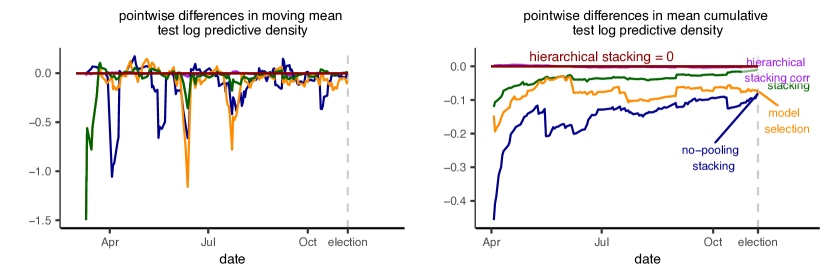
Figure 13: Same pointwise model comparisons as in Figure 7, except this time all model averaging and selection methods are trained using the previous 60 days rather than 4 weeks on each backtesting day. The pattern remains similar.

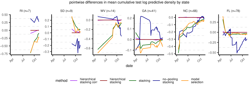
Figure 14: Log predictive density of the combined model in three small states (in the number of available state polls $n$, RI, SD, WV) and three swing states (GA, NC, FL). We fix the uncorrelated hierarchical stacking to be constant zero as a reference. The number in the bracket is the total number of polls in that state. With a large number of state polls available, for example, close to election day in Florida and North Carolina, no-pooling stacking performs well. With fewer polls, no-pooling stacking is unstable, as can be seen in Rhode Island, South Dakota, West Virginia, and the early part of Georgia plots. Hierarchical stacking alleviates this instability, while retaining enough flexibility for a good performance with large data come in.

References

- Abramowitz, (2008) Abramowitz, A. I. (2008). Forecasting the 2008 presidential election with the time-for-change model. Political Science and Politics, 41:691–695.
- Bernardo and Smith, (1994) Bernardo, J. M. and Smith, A. F. (1994). Bayesian Theory. Wiley, Chichester.
- Bhatt et al., (2017) Bhatt, S., Cameron, E., Flaxman, S. R., Weiss, D. J., Smith, D. L., and Gething, P. W. (2017). Improved prediction accuracy for disease risk mapping using Gaussian process stacked generalization. Journal of The Royal Society Interface, 14.
- Breiman, (1996) Breiman, L. (1996). Stacked regressions. Machine Learning, 24:49–64.
- Breiman, (2001) Breiman, L. (2001). Statistical modeling: the two cultures. Statistical Science, 16:199–231.
- Bürkner et al., (2020) Bürkner, P.-C., Gabry, J., and Vehtari, A. (2020). Approximate leave-future-out cross-validation for Bayesian time series models. Journal of Statistical Computation and Simulation, 90:2499–2523.
- Clarke, (2003) Clarke, B. (2003). Comparing Bayes model averaging and stacking when model approximation error cannot be ignored. Journal of Machine Learning Research, 4:683–712.
- Clyde and Iversen, (2013) Clyde, M. and Iversen, E. S. (2013). Bayesian model averaging in the M-open framework. In Bayesian Theory and Applications, pages 483–498. Oxford University Press.
- Fushiki, (2020) Fushiki, T. (2020). On the selection of the regularization parameter in stacking. Neural Processing Letters, pages 1–12.
- Gelman and Pardoe, (2006) Gelman, A. and Pardoe, I. (2006). Bayesian measures of explained variance and pooling in multilevel (hierarchical) models. Technometrics, 48:241–251.
- Gelman et al., (2020) Gelman, A., Vehtari, A., Simpson, D., Margossian, C. C., Carpenter, B., Yao, Y., Kennedy, L., Gabry, J., Bürkner, P.-C., and Modrák, M. (2020). Bayesian workflow. arXiv:2011.01808.
- Ghasemian et al., (2020) Ghasemian, A., Hosseinmardi, H., Galstyan, A., Airoldi, E. M., and Clauset, A. (2020). Stacking models for nearly optimal link prediction in complex networks. Proceedings of the National Academy of Sciences, 117:23393–23400.
- Heidemanns et al., (2020) Heidemanns, M., Gelman, A., and Morris, G. E. (2020). An updated dynamic Bayesian forecasting model for the US presidential election. Harvard Data Science Review, 2.
- Heiner et al., (2019) Heiner, M., Kottas, A., and Munch, S. (2019). Structured priors for sparse probability vectors with application to model selection in Markov chains. Statistics and Computing, 29:1077–1093.
- Hoeting et al., (1999) Hoeting, J. A., Madigan, D., Raftery, A. E., and Volinsky, C. T. (1999). Bayesian model averaging: a tutorial. Statistical Science, pages 382–401.
- Jacobs et al., (1991) Jacobs, R. A., Jordan, M. I., Nowlan, S. J., and Hinton, G. E. (1991). Adaptive mixtures of local experts. Neural Computation, 3:79–87.
- Jordan and Jacobs, (1994) Jordan, M. I. and Jacobs, R. A. (1994). Hierarchical mixtures of experts and the EM algorithm. Neural Computation, 6:181–214.
- Kamary et al., (2019) Kamary, K., Mengersen, K., Robert, C. P., and Rousseau, J. (2019). Testing hypotheses via a mixture estimation model. arXiv:1412.2044.
- Le and Clarke, (2017) Le, T. and Clarke, B. (2017). A Bayes interpretation of stacking for -complete and -open settings. Bayesian Analysis, 12:807–829.
- LeBlanc and Tibshirani, (1996) LeBlanc, M. and Tibshirani, R. (1996). Combining estimates in regression and classification. Journal of the American Statistical Association, 91:1641–1650.
- Linzer, (2013) Linzer, D. A. (2013). Dynamic Bayesian forecasting of presidential elections in the states. Journal of the American Statistical Association, 108:124–134.
- Meng and van Dyk, (1999) Meng, X.-L. and van Dyk, D. A. (1999). Seeking efficient data augmentation schemes via conditional and marginal augmentation. Biometrika, 86:301–320.
- Neal, (1998) Neal, R. M. (1998). Regression and classification using Gaussian process priors. In Bernardo, J., Berger, J. O., Dawid, A. P., and Smith, A. F. M., editors, Bayesian Statistics, volume 6, pages 475–501. Oxford University Press.
- Piironen and Vehtari, (2017) Piironen, J. and Vehtari, A. (2017). Comparison of Bayesian predictive methods for model selection. Statistics and Computing, 27(3):711–735.
- Pirš and Štrumbelj, (2019) Pirš, G. and Štrumbelj, E. (2019). Bayesian combination of probabilistic classifiers using multivariate normal mixtures. Journal of Machine Learning Reserach, 20:1–18.
- Polson and Scott, (2011) Polson, N. G. and Scott, S. L. (2011). Data augmentation for support vector machines. Bayesian Analysis, 6:1–23.
- Reid and Grudic, (2009) Reid, S. and Grudic, G. (2009). Regularized linear models in stacked generalization. In International Workshop on Multiple Classifier Systems, pages 112–121.
- Şen and Erdogan, (2013) Şen, M. U. and Erdogan, H. (2013). Linear classifier combination and selection using group sparse regularization and hinge loss. Pattern Recognition Letters, 34:265–274.
- Shimodaira, (2000) Shimodaira, H. (2000). Improving predictive inference under covariate shift by weighting the log-likelihood function. Journal of Statistical Planning and Inference, 90:227–244.
- Sill et al., (2009) Sill, J., Takács, G., Mackey, L., and Lin, D. (2009). Feature-weighted linear stacking. arXiv:0911.0460.
- Stan Development Team, (2020) Stan Development Team (2020). Stan Modeling Language Users Guide and Reference Manual. Version 2.25.0, http://mc-stan.org.
- Sugiyama et al., (2007) Sugiyama, M., Krauledat, M., and Müller, K.-R. (2007). Covariate shift adaptation by importance weighted cross validation. Journal of Machine Learning Research, 8:985–1005.
- Sugiyama and Müller, (2005) Sugiyama, M. and Müller, K.-R. (2005). Input-dependent estimation of generalization error under covariate shift. Statistics and Decisions, 23:249–280.
- Svensën and Bishop, (2003) Svensën, M. and Bishop, C. M. (2003). Bayesian hierarchical mixtures of experts. In Uncertainty in Artificial Intelligence.
- Tracey and Wolpert, (2016) Tracey, B. D. and Wolpert, D. H. (2016). Reducing the error of Monte Carlo algorithms by learning control variates. In Conference on Neural Information Processing Systems.
- Vehtari et al., (2020) Vehtari, A., Gabry, J., Magnusson, M., Yao, Y., Bürkner, P.-C., Paananen, T., and Gelman, A. (2020). loo: Efficient leave-one-out cross-validation and WAIC for bayesian models. R package version 2.4.1, {https://mc-stan.org/loo/}.
- Vehtari et al., (2017) Vehtari, A., Gelman, A., and Gabry, J. (2017). Practical Bayesian model evaluation using leave-one-out cross-validation and WAIC. Statistics and Computing, 27:1413–1432.
- Vehtari and Ojanen, (2012) Vehtari, A. and Ojanen, J. (2012). A survey of Bayesian predictive methods for model assessment, selection and comparison. Statistics Surveys, 6:142–228.
- Vehtari et al., (2019) Vehtari, A., Simpson, D., Gelman, A., Yao, Y., and Gabry, J. (2019). Pareto smoothed importance sampling. arXiv:1507.02646.
- Waterhouse et al., (1996) Waterhouse, S., MacKay, D., and Robinson, T. (1996). Bayesian methods for mixtures of experts. In Advances in Neural Information Processing Systems.
- Wolpert, (1992) Wolpert, D. H. (1992). Stacked generalization. Neural Networks, 5:241–259.
- Yang and Dunson, (2014) Yang, Y. and Dunson, D. B. (2014). Minimax optimal Bayesian aggregation. arXiv:1403.1345.
- Yao, (2019) Yao, Y. (2019). Bayesian aggregation. arXiv:1912.11218.
- Yao et al., (2020) Yao, Y., Vehtari, A., and Gelman, A. (2020). Stacking for non-mixing Bayesian computations: The curse and blessing of multimodal posteriors. arXiv:2006.12335.
- Yao et al., (2018) Yao, Y., Vehtari, A., Simpson, D., and Gelman, A. (2018). Using stacking to average Bayesian predictive distributions (with discussion). Bayesian Analysis, 13:917–1007.
- Zhang and Zhou, (2011) Zhang, L. and Zhou, W.-D. (2011). Sparse ensembles using weighted combination methods based on linear programming. Pattern Recognition, 44:97–106.