Hessian-Aware Pruning and Optimal Neural Implant

Abstract

Pruning is an effective method to reduce the memory footprint and FLOPs associated with neural network models. However, existing structured-pruning methods often result in significant accuracy degradation for moderate pruning levels. To address this problem, we introduce a new Hessian Aware Pruning (HAP) method coupled with a Neural Implant approach that uses second-order sensitivity as a metric for structured pruning. The basic idea is to prune insensitive components and to use a Neural Implant for moderately sensitive components, instead of completely pruning them. For the latter approach, the moderately sensitive components are replaced with with a low rank implant that is smaller and less computationally expensive than the original component. We use the relative Hessian trace to measure sensitivity, as opposed to the magnitude based sensitivity metric commonly used in the literature. We test HAP for both computer vision tasks and natural language tasks, and we achieve new state-of-the-art results. Specifically, HAP achieves less than $0.1\%$/$0.5\%$ degradation on PreResNet29/ResNet50 (CIFAR-10/ImageNet) with more than 70%/50% of parameters pruned. Meanwhile, HAP also achieves significantly better performance (up to 0.8% with 60% of parameters pruned) as compared to gradient based method for head pruning on transformer-based models. The framework has been open sourced and available online [1].

1 Introduction

There has been a significant increase in the computational resources required for Neural Network (NN) training and inference. This is in part due to larger input sizes (e.g., higher image resolution) as well as larger NN models requiring more computation with a significantly larger memory footprint. The slowing down of Moore’s law, along with challenges associated with increasing memory bandwidth, has made it difficult to deploy these models in practice. Often, the inference time and associated power consumption is orders of magnitude higher than acceptable ranges. This has become a challenge for many applications, e.g., health care and personalized medicine, which have restrictions on uploading data to cloud servers, and which have to rely on local servers with limited resources. Other applications include inference on edge devices such as mobile processors, security cameras, and intelligent traffic control systems, all of which require real-time inference. Importantly, these problems are not limited to edge devices, and state-of-the-art models for applications such as speech recognition, natural language processing, and recommendation systems often cannot be efficiently performed even on high-end servers.

A promising approach to address this is pruning.  [44, 43, 7, 71, 33, 15, 51, 36, 48, 65, 61, 57, 12, 14, 75, 42, 32, 60, 74, 13, 35], However, an important challenge is determining which parameters are insensitive to the pruning process. A brute-force method is not feasible since one has to test each parameter in the network separately and measure its sensitivity. The seminal work of [33] proposed Optimal Brain Damage (OBD), a second-order based method to determine insensitive parameters. However, this approach requires pruning the parameters one at a time, which is time-consuming. To address this problem, we propose a simple, yet effective, modification of OBD by using the Hessian trace to prune a group of parameters along with a low rank Neural Implant. In more detail, our contributions are as follows:

• We propose HAP, a Hessian Aware Pruning method that uses a fast second-order metric to find insensitive parameters in a NN model. In particular, we use the average Hessian trace to weight the magnitude of the parameters in the NN. Parameters with large second-order sensitivity remain unpruned, and those with relatively small sensitivity are pruned. In contrast to OBD [33], HAP finds groups of insensitive parameters, which is faster than pruning a single parameter at a time. Details of the HAP method are discussed in Section 3.

• We propose a novel Neural Implant (denoted by HAP+Implant) technique to alleviate accuracy degradation. In this approach, we replace moderately sensitive model components with a low rank implant. The model along with the implant is then fine-tuned. We find that this approach helps boost the accuracy. For details, see Section 3.2.

• We perform detailed empirical testing and show that HAP achieves 94.3% accuracy ($<0.1\%$ degradation) on PreResNet29 (CIFAR-10), with only 31% parameters left (Figure 2). In comparison to EigenDamage, a recent second-order pruning method, we achieve up to 1.2% higher accuracy with fewer parameters and FLOPs (Figure 2). Moreover, for ResNet50, HAP achieves 75.1% top-1 accuracy (0.5% degradation) on ImageNet, with only half of the parameters left (Table 3.2). In comparison to prior state-of-the-art HRank [37], HAP achieves up to 2% higher accuracy with fewer parameters and FLOPs (Table 3.2). For head pruning of RoBERTa on MRPC/QNLI, HAP achieves up to 0.82%/0.89% higher accuracy than the gradient based method [49] (Table 6).

• We perform detailed ablation experiments to illustrate the efficacy of the second-order sensitivity metric. In particular, we compare the second-order sensitivity with a random method, and a reverse-order in which the opposite order sensitivity order given by HAP is used. In all cases, HAP achieves higher accuracy (Table 4.4).

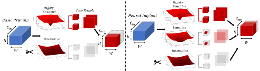
Figure 1: (Left) The HAP method is a structured pruning method that prunes channels based on their second-order sensitivity, which measured flatness/sharpness of loss landscape. Channels are sorted based on this metric, and only insensitive channels are pruned. (Right) Similar to other structured-pruning methods, HAP at large pruning ratios results in accuracy degradation. This because one has to inevitably prune moderately sensitive channels at high pruning ratios, which may contain individual neurons that are very sensitive. The removal of the entire channel, along with the sensitive neurons results in accuracy degradation. To address this, we propose HAP+Implant method, where such channels are replaced with a light-weight, low-rank Neural Implant.

2 Related work

Several different approaches have been proposed to make NN models more efficient by making them more compact, faster, and more energy efficient. These efforts could be generally categorized as follows: (i) efficient NN design [27, 24, 55, 23, 72, 46]; (ii) hardware-aware NN design [11, 62, 5, 45, 66, 56]; (iii) quantization [63, 28, 26, 29, 9, 8]; (iv) distillation [22, 50, 69, 53]; and (v) pruning.

Here we briefly discuss the related work on pruning, which can be broadly categorized into: unstructured pruning [7, 34, 64, 52]; and structured pruning [44, 19, 70, 38, 25, 73]. Unstructured pruning prunes out neurons without any structure. However, this leads to sparse matrix operations which are hard to accelerate and are typically memory-bounded  [4, 10]. This can be addressed with structured pruning, where an entire matrix operation (e.g., an output channel) is removed. However, the challenge here is that high degrees of structured pruning often leads to significant accuracy degradation.

In both approaches, the key question is to find which parameters to prune. A simple and popular approach is magnitude-based pruning. In this approach, the magnitude of parameters is used as the pruning metric. The assumption here is that small parameters are not important and can be removed. A variant of this approach was used in [41], where the scaling factor of the batch normalization layer is used as the sensitivity metric. In particular, channels with smaller scaling factors (or output values) are considered less important and got pruned. Another variation is proposed by [36], where channel-wise summation over weights is used as the metric. Other methods have been proposed as alternative sensitivity metrics. For instance, [37] uses channel rank as sensitivity metric; [21] uses a LASSO regression based channel selection criteria; and [20] uses the geometric median of the convolutional filters. An important problem with magnitude-based pruning methods is that parameters with small magnitudes can actually be quite sensitive. It is easy to see this through a second-order Taylor series expansion, where the perturbation is dependent on not just the weight magnitude but also the Hessian [33]. In particular, small parameters with large Hessian could in fact be very sensitive, as opposed to large parameters with small Hessian (here, we are using small/large Hessian loosely; the exact metric to measure is given by the second-order perturbation in Eq. 3). For this reason, OBD [33] proposes to use the Hessian diagonal as the sensitivity metric. The follow up work of Optimal Brain Surgeon (OBS) [17, 16] used a similar method, but considered off-diagonal Hessian components, and showed a correlation with inverse Hessian. One important challenge with these methods is that pruning has to be performed one parameter at a time. The recent work of [7] extends this to layer-wise pruning in order to reduce the cost of computing Hessian information for one parameter at a time. However, this method can result in unstructured pruning. Another second-order pruning method is EigenDamage [60], where the Gauss-Newton operator is used instead of Hessian. In particular, the authors use Kronecker products to approximate the GN operator. Our findings below show that using the average Hessian trace method significantly outperforms EigenDamage. We also find that it is very helpful to replace moderately sensitive layers with a low rank Neural Implant, instead of completely pruning them, as discussed next.

3 Methodology

Here, we focus on supervised learning tasks, where the nominal goal is to minimize the empirical risk by solving the following optimization problem:

$$\small L(w)=\frac{1}{N}\sum\nolimits_{i=1}^{N}l(x_{i},y_{i},w),$$ (1)

where $w\in{\mathbb{R}}^{n}$ is the trainable model parameters, $l(x_{i},y_{i},w)$ is the loss for the input datum $x_{i}$, where $y_{i}$ is the corresponding label, and $N$ is the training set cardinality. For pruning, we assume that the model is already trained and converged to a local minima which satisfies the first and second-order optimality conditions (that is, the gradient $\nabla_{w}L(w)=0$, and the Hessian is Positive Semi-Definite (PSD), $\nabla^{2}_{w}L(w)\succcurlyeq 0$). The problem statement is to prune (remove) as many parameters as possible to reduce the model size and FLOPs to a target threshold with minimal accuracy degradation.

We first start with a general description of the problem and then derive our method. Let $\Delta w\in{\mathbb{R}}^{n}$ denote the pruning perturbation such that the corresponding weights become zero (that is $w+\Delta w=0$). We denote the corresponding change of loss as $\Delta L$:

$$\small\Delta L=L(w+\Delta w)-L(w)=g^{T}\Delta w+\frac{1}{2}\Delta w^{T}H\Delta w+O(||\Delta w||^{3}).$$ (2)

where the second equation comes from Taylor series expansion. Here $g\in{\mathbb{R}}^{n}$ denotes the gradient of loss function $L$ w.r.t. weights $w$, and $H\in{\mathbb{R}}^{n\times n}$ is the corresponding Hessian operator (i.e. second-order derivative). For a pretrained neural network that has already converged to a local minimum, we have $g=0$, and the Hessian is a PSD matrix. As in prior work [17], we assume higher-order terms, e.g., $O(||\Delta w||^{3})$, in Eq. 2 can be ignored.

The pruning problem is to find the set of weights that result in minimum perturbation to the loss ($\Delta L$). This leads to the following constrained optimization problem:

$$\scriptsize\begin{split}\min_{\Delta w}\frac{1}{2}\Delta w^{T}H\Delta w&=\frac{1}{2}\begin{pmatrix}\Delta w_{p}\\ \Delta w_{l}\end{pmatrix}^{T}\begin{pmatrix}H_{p,p}&H_{p,l}\\ H_{l,p}&H_{l,l}\end{pmatrix}\begin{pmatrix}\Delta w_{p}\\ \Delta w_{l}\end{pmatrix},\\ &\text{s.t.}\quad\Delta w_{p}+w_{p}=0.\end{split}$$ (3)

Here, we denote the channels that are pruned with $p$ as the subscript (e.g. $w_{p}\in{\mathbb{R}}^{p}$), and denote the remaining parameters with $l$ as the subscript (e.g. $w_{l}\in{\mathbb{R}}^{n-p}$). Similarly, we use $\Delta w_{p}$ and $\Delta w_{l}$ to denote the corresponding perturbations. Note that $\Delta w_{p}=-w_{p}$ since $p$-channels are pruned. Moreover, $H_{l,p}$ denotes the cross Hessian w.r.t. $l$-channels and $p$-channels (and similarly $H_{p,p}$ and $H_{l,l}$ are Hessian w.r.t. pruned and unpruned parameters). Using Lagrangian method, we can finally get (see section A for more details):

$$\small\frac{1}{2}\Delta w^{T}H\Delta w=\frac{1}{2}w_{p}^{T}(H_{p,p}-H_{p,l}H_{l,l}^{-1}H_{l,p})w_{p}.$$ (4)

Eq. 4 gives us the perturbation to the loss when a set of parameters $w_{p}$ is removed. It should be noted that OBS [17] and L-OBS [7], where OBS is applied for each layer under the assumption of cross-layer independence, is a degenerate case of Eq. 4 for the special case of $w_{p}\in{\mathbb{R}}^{1}$. Next we discuss how this general formulation can be simplified.

3.1 Hessian-aware Pruning

There are three major disadvantages with OBS. First, computing Eq. 4 requires computing (implicitly) information from the inverse Hessian, $H_{l,l}^{-1}$. This can be costly, both in terms of computations and memory (even when using matrix-free randomized methods). The work of L-OBS [7] attempted to address this challenge by ignoring cross-layer dependencies, but it still requires computing block-diagonal inverse Hessian information, which can be costly. Second, in both OBS and L-OBS, one has to measure this perturbation for all the parameters separately, and then prune those parameters that result in the smallest perturbation. This can have a high computational cost, especially for deep models with many parameters. Third, this pruning method results in unstructured pruning, which is difficult to accelerate with current hardware architectures. In the OBD [33] method the first problem does not exist as the the Hessian is approximated as a diagonal operator, without the need to compute inverse Hessian:

$$\small\begin{split}\frac{1}{2}\Delta w^{T}H\Delta w&\approx\frac{1}{2}w_{p}^{T}Diag(H_{p,p})w_{p}.\end{split}$$ (5)

Here $Diag(H_{p,p})$ denotes the diagonal elements of $H_{p,p}$. However, the second and third of these disadvantages still remain with OBD.

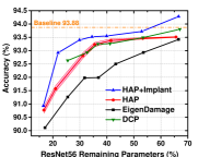
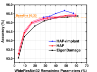
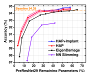
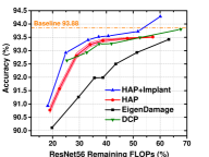
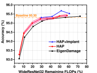
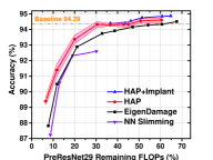
Figure 2: Comparison of accuracy with different pruning ratios among HAP+Implant, HAP, NN Slimming, EigenDamage, and DCP, on the CIFAR-10 dataset, for ResNet56, WideResNet32, and PreResNet29. (Top) Remaining parameters in the network after pruning is used for x-axis. (Bottom) Remaining FLOPs in the network after pruning is used for x-axis. HAP consistently outperforms EigenDamage and NN Slimming, and HAP+Implant boosts performance for moderate pruning ratios and surpasses DCP.

To address the second and third of these disadvantages, we propose to group the parameters and to compute the corresponding perturbation when that group is pruned, rather than computing the perturbation for every single parameter separately. Note that this can also address the third disadvantage, since pruning a group of parameters (for example parameters in a convolution channel) results in structured pruning. This can be achieved by considering the Hessian as a block diagonal operator, and then approximating each block with a diagonal operator, with Hessian trace as the diagonal entries. In particular, we use the following approximation:

$$\small\begin{split}\frac{1}{2}\Delta w^{T}H\Delta w&=\frac{1}{2}w_{p}^{T}[H^{-1}]_{p,p}^{-1}w_{p}\approx\frac{1}{2}w_{p}^{T}\frac{Trace(H_{p,p})}{p}w_{p}=\frac{Trace(H_{p,p})}{2p}\|w_{p}\|_{2}^{2},\end{split}$$ (6)

where $Trace(H_{p,p})$ denotes the trace of the block diagonal Hessian (the corresponding Hessian block for pruned parameters $H_{p,p}$). The Hessian can be computed very efficiently with randomized numerical linear algebra methods, in particular Hutchinson’s method [3, 2, 67, 68]. Importantly, this approach requires computing only the application of the Hessian to a random input vector. This has the same cost as back-propagating the gradient [67, 68]. (Empirically, in our experiments corresponding to ResNet50 on ImageNet, the longest time for computing this trace was three minutes.) A similar approach was proposed by [8] in the context of quantization.

In more detail, HAP performs structured pruning by grouping the parameters and approximating the corresponding Hessian as a diagonal operator, with the average Hessian trace of that group as its entries. For a convolutional network, this group can be an output channel. We found that this simple modification results in a fast and efficient pruning method that when combined with the Neural Implant approach exceeds state-of-the-art. This is discussed next.

3.2 Hessian-aware Neural Implant

In HAP, we sort the channels from most sensitive to least sensitive (based on Eq. 6). For a target model size or FLOPs budget, one has then to prune by starting from insensitive channels. This approach works well, as long as all these channels are extremely insensitive. However, in practice, some of the sorted channels will exhibit some level of sensitivity. Entirely pruning these channels, and leaving the rest of the sensitive ones unpruned, can result in significant accuracy degradation. This is one of the major problems with structured pruning methods, as very few groups of parameters are completely insensitive. When those are pruned, the remaining groups/set of parameters always include some subset of highly sensitive neurons that if pruned, would result in high accuracy loss.

Here, we propose an alternative strategy to replace moderately sensitive parameter groups with a low rank Neural Implant. The basic idea is to prune insensitive layers completely, but detect the moderately sensitive layers, and instead of completely removing all of its parameters (which can contain some sensitive ones as discuss above), replace them with a low rank decomposition. As an example, a spatial convolution could be replaced with a new point-wise convolution that has smaller parameters and flops. One could also consider other types of low rank decomposition (e.g. CP/Tucker decomposition, depth-wise/separable convolution,etc). However, for simplicity we only use a pointwise convolution implant in this paper.

After the implant, the model is fine-tuned to recover accuracy. We denote this approach as HAP+Implant, which is schematically illustrated in Figure 1. In summary, we use the Hessian metric in Eq. 6, and then we apply a Neural Implant to the most sensitive channels to be pruned.

We have to emphasize that many prior works have investigated low-rank matrix approximation [47]. However, existing methods for NN pruning replace all or part of the model, irrespective of their sensitivity, whereas in our approach we perform a targeted low-rank approximation, and only replace the sensitive parts of the model, quantified through the Hessian in Eq. 6. We empirically found that this approach is quite effective, especially for moderate pruning ratios, as discussed next.

Table 1: Comparison between HAP and other pruning methods on CIFAR-10. Here, VGG16 denotes the baseline used in HRank [37], and VGG16-HAP denotes the baseline used by HAP method. As one can see, HAP consistently outperforms other pruning methods, even though its pruned models have fewer parameters (Param.) and FLOPs.

Method Acc.(%) Param.(%) FLOPs(%) VGG16 93.96 100.0 100.0 VGG16-HAP 93.88 100.0 100.0 L1[36] 93.40 36.0 65.7 SSS[25] 93.02 26.2 58.4 VarP[73] 93.18 26.7 60.9 HRank[37] 93.43 17.1 46.5 GAL-0.05[39] 92.03 22.4 60.4 HRank[37] 92.34 17.9 34.7 GAL-0.1[39] 90.73 17.8 54.8 HAP 93.66 10.1 29.7 HRank[37] 91.23 8.0 23.5 HAP 93.37 5.1 20.3 HAP 91.22 1.6 7.5

Table 2: Comparison of FLOPs and accuracy on CIFAR-10 using ResNet56 for different pruning methods. We report the baseline accuracy used in each work, as well as the corresponding final accuracy after pruning. For ease of comparison, we also report the accuracy drop (Acc. $\downarrow$) w.r.t. each baseline. As one can see, HAP and HAP+Implant consistently outperform other work reported in the literature.

Method Base-acc. Final-acc. Acc. $\downarrow$ FLOPs (%) CP[21] 92.80 91.80 1.00 50.0 AMC[19] 92.80 91.90 0.90 50.0 FPGM[20] 93.59 93.26 0.33 47.4 LFPC[18] 93.59 93.24 0.35 47.1 HAP+Implant 93.88 93.55 0.33 40.7 GAL-0.8[39] 93.26 90.36 2.90 39.8 HRank[37] 93.26 90.72 2.54 25.9 HAP 93.88 91.57 2.31 21.0 HAP+Implant 93.88 92.92 0.96 23.9

4 Results

4.1 Experimental Settings

Computer Vision. For evaluating the performance of HAP, we conduct experiments for image classification on CIFAR-10 (ResNet56/WideResNet32/PreResNet29/VGG16) and ImageNet (ResNet50). Our main target comparison for HAP (without Implant) is EigenDamage, a recent second-order pruning method. For fair comparison, we use the same pretrained model used by EigenDamage when available (WideResNet32 on Cifar-10), and otherwise train the model from scratch (ResNet56, VGG16, and PreResNet29 on Cifar-10). For all cases, we ensure comparable baseline accuracy, and when not possible, we report the baseline used by other methods. For comparison we consider a wide range of pruning ratios, and consider validation accuracy, FLOPs, and parameter size as the metrics. The goal is to achieve higher accuracy with lower FLOPs/parameter size.

Natural Language Understanding. We use RoBERTa-base [40], which consists of 12 attention heads for each of 12 Transformer encoder layers, as the baseline model. It has been explored in [49] that not all heads in Transformer architectures are equally important and thus a great portion of them can be removed without degrading the accuracy.

4.2 HAP Results on CIFAR-10

We first start with evaluating HAP without Neural Implant, and then discuss the specific improvement of using Neural Implant. The results on CIFAR-10 for different pruning ratios and various models are presented in Figure 2. In particular, we report both the validation accuracy versus remaining parameters after pruning, as well as validation accuracy versus the FLOPs. For comparison, we also plot the performance of NN slimming [41], EigenDamage [60] and DCP [75] for different pruning ratios. For all the points that we compare, HAP achieves higher accuracy than EigenDamage, even for cases with fewer parameters/FLOPs. We generally observe that the difference between HAP and EigenDamage is more noticeable for higher pruning ratios (i.e., fewer remaining parameter). This is expected, since small amounts of pruning does not lead to significant accuracy degradation, while higher pruning ratios are more challenging. In particular, when the parameter remaining percentage is around 35% (i.e., 65% of the parameters are pruned), HAP achieves 93.2% accuracy, which is 1.24% higher than EigenDamage, with fewer FLOPs (34.0% versus 38.7% for EigenDamage). We observe a similar trend on WideResNet32, where HAP consistently outperforms EigenDamage.

We also plot the performance of DCP, which is not a second-order method, but is known to achieve good pruning accuracy. HAP achieves higher accuracy as compared to NN slimming, and comparable accuracy to DCP. As for the latter, the benefit of HAP is that we do not need to perform any greedy channel selection and the entire Hessian calculation and channel selection is performed in one pass.

For PreResNet29, we also compare with NN Slimming [41], to compare with prior reported results on this model. We observe that HAP achieves up to 6% higher accuracy as compared to NN Slimming method, and slightly higher accuracy as compared to EigenDamage. It is interesting to note that HAP can keep the accuracy the same as baseline, up to pruning 70% of the parameters (corresponding to 30% remaining parameters in Figure 2).

We also present results on VGG16 and compare with other works in the literature, including GAL [39], HRank [37], and VarP [73], as reported in Table 3.2. Here, we consistently achieve higher accuracy. In particular, HAP with 29.7% FLOPs and 10.1% parameters achieves the highest accuracy (despite using a pretrained model with lower baseline accuracy). Similarly, HAP with 20.3% FLOPs and 5.1% parameters achieves 93.37% accuracy, with less than $2\times$ FLOPs and $3\times$ fewer parameters as compared to HRank in the same block. For extreme pruning, HAP achieves 91.22% accuracy with only 1.6% of the parameters remaining. To the best of our knowledge, this level of aggressive pruning, while maintaining such high accuracy, has not been reported in the literature.

It is interesting to visualize how HAP performs channel selection using the second-order sensitivity discussed in Sec. 3.1, and the result can be found in section E

4.3 Neural Implant Results on CIFAR-10

Despite HAP’s competitive results as compared to prior pruning methods, it still has lower accuracy as compared to baseline. This is known problem and shortcoming of structured pruning methods. We propose to use a low rank Neural Implant to address this problem, and find it particularly helpful for moderate levels of structured pruning. In particular, for the CNNs tested in this paper we replace sensitive $3\times 3$ spatial convolutions with a pointwise convolution. This replacement still reduces the number of parameters for the $3\times 3$ convolution by a factor of $9\times$.

We repeated the previous experiments with this approach, and report the results in Figure 2 (blue line). We observe that HAP+Implant consistently achieves better performance than HAP for both the same parameter size (first row) and the same FLOPs (second row), which also surpasses the performance of DCP [75] that has a competitive result with HAP.

For some cases, the performance of the pruned network slightly exceeds the baseline accuracy. In particular, for ResNet56, we observe up to 1.5% higher accuracy as compared to HAP, and up to 2% higher accuracy as compared to EigenDamage. We observe a similar trend for both WideResNet32/PreResNet29, where HAP+Implant consistently performs better than both HAP and EigenDamage.

It should be noted that the gains from HAP+Implant diminish for higher pruning ratios (around 20% remaining parameters for ResNet56, and around 30% remaining for WideResNet32/PreResNet29). This is expected, since there is a trade-off associated with adding the Neural Implant. While the implant helps reduce the information loss from completely removing sensitive channels, it does so by adding additional parameters. As such, we actually have to enforce a larger pruning ratio to meet a target model size. As the channels are sorted based on their sensitivity (from Eq. 6), this means that we have to prune the next set of more sensitive channels to satisfy the target. However, if such channels have much higher sensitivity, then that can actually degrade the performance. This is what happens for extreme pruning cases, since most of the remaining parameters will be highly sensitive; and, as such, the gains achieved by the Neural Implant will not be enough.

In addition to parameter percentage, we also compare HAP+Implant results based on remaining FLOPs with other methods reported in the literature. This is shown in Table 3.2. As one can see, with a high remaining FLOPs percentage, HAP+Implant can reach 93.55% accuracy with only 0.33% degradation as compared with the corresponding pretrained baseline model. It should be noted that state-of-the-art methods such as FPGM [20] and LFPC [18] requires 6.4% more FLOPs to reach comparable performance. Moreover, when the target percentage of remaining FLOPs is small, HAP+Implant only incurs 0.96% accuracy degradation as compared with 2.31% for HAP and 2.54% for HRank [37] (with comparable FLOPs and baseline accuracy).

4.4 HAP Results on ImageNet

We also test HAP on ImageNet using ResNet50, and report the results in Table 4.4. We compare with several previous structured pruning methods including SSS [25], CP [21], ThiNet [44], and HRank [37]. It should be noted that the accuracy of our pretrained baseline is slightly lower than HRank, yet our HAP method still achieves higher accuracy. For instance, in all cases, HAP achieves higher accuracy with smaller number of parameters as compared to all prior work reported on ResNet50. The highest difference corresponds to 34.74% remaining parameters (i.e., pruning 65.26% of parameters), where HAP has 2% higher Top-1 accuracy with 19.26% fewer parameters as compared to HRank (although for fairness our FLOPs are slightly larger). We observe a consistent trend even for high pruning ratios. For example, with 20.47% remaining parameters, HAP still has more than 2% higher accuracy as compared to HRank. We should also note that despite using second-order information, HAP is quite efficient, and the end-to-end Hessian calculations were completed three minutes on a single RTX-6000 GPU.

Table 3: Comparison between HAP and HAP+Implant, and other state-of-the-art pruning methods on ImageNet. Here, ResNet50 is the baseline used in HRank [37]’s table, while ResNet50-HAP is the baseline used by HAP.

Method Top-1 Param.(%) FLOPs(%) ResNet50-MetaP 76.16 100.0 100.0 ResNet50 76.15 100.0 100.0 ResNet50-HAP 75.62 100.0 100.0 SSS-32[25] 74.18 72.94 68.95 CP[21] 72.30 - 66.75 GAL-0.5[39] 71.95 83.14 56.97 MetaP[42] 72.27 61.35 56.36 HRank[37] 74.98 63.33 56.23 HAP 75.12 55.41 66.18 HAP+Implant 75.36 53.74 55.49 GDP-0.6[38] 71.19 - 45.97 GDP-0.5[38] 69.58 - 38.39 SSS-26[25] 71.82 61.18 56.97 GAL-1[39] 69.88 57.53 38.63 GAL-0.5-joint[39] 71.82 75.73 44.99 HRank[37] 71.98 54.00 37.90 HAP 74.00 34.74 40.44 ThiNet-50[44] 68.42 33.96 26.89 GAL-1-joint[39] 69.31 40.04 27.14 HRank[37] 69.10 32.43 23.96 MetaP[42] 70.07 41.44 25.69 HAP 71.18 20.47 32.85

Table 4: Ablation study on the sensitivity metric. R-HAP denotes pruning by reversely using sensitivity in HAP. Random is conducted by randomly allocating channel-wise sensitivity.

Method Acc. Param.(%) FLOPs(%) Channel R-HAP 89.77 47.48 46.98 65 Random 93.12 45.60 46.68 60 Magnitude 93.29 61.82 39.29 55 HAP 93.38 41.53 38.74 50 R-HAP 89.97 42.85 39.99 60 Random 92.21 36.01 33.99 50 Magnitude 92.99 56.15 34.97 50 HAP 93.23 35.50 33.99 45 R-HAP 88.83 27.15 30.61 50 Random 90.95 29.64 31.32 40 Magnitude 92.45 47.28 28.97 42.2 HAP 92.81 31.08 28.85 40 R-HAP 88.18 23.34 28.04 45 Random 90.18 25.33 25.69 30 Magnitude 91.65 38.25 22.93 35 HAP 92.06 22.05 22.86 31

Table 5: Comparison of HAP and the gradient-based [49] heads pruning methods for RoBERTa-base, evaluated on MRPC and QNLI. As an evaluation metric, we report accuracy for QNLI and the average of accuracy and F1 score for MRPC.

Parameter (%)	100	80	60	50	40
Gradient-based [49]	92.06	92.19	89.52	89.36	89.07
HAP	92.06	91.97	90.74	90.43	89.89
Diff	0.00	-0.22	+1.22	+1.07	+0.82

(a) MRPC

Parameter (%)	100	80	60	50	40
Gradient-based [49]	93.12	92.4	91.78	91.71	91.38
HAP	93.12	93.30	92.93	92.59	92.27
Diff	0.00	+0.90	+1.15	+0.88	+ 0.89

(b) QNLI

Table 6: Hessian Aware Low Rank (Neural Implant) vs Low Rank. Ablation study on Hessian aware Neural Implant. The R-HAP+Implant uses low rank replacement without using Hessian information. Specially, the Neural Implant is applied on channels that are most sensitive.

ResNet56/Cifar10 Acc. Param.(%) FLOPs(%) Low Rank 90.79 39.56 40.33 HAP+Implant 93.52 34.49 37.15 Low Rank 90.34 34.39 37.24 HAP+Implant 93.40 29.87 33.20 Low Rank 89.83 23.05 25.16 HAP+Implant 92.92 21.92 24.90

4.5 HAP Results on RoBERTa

Additionally, we show in this section that our HAP method can be applied to Transformer [58] architectures to prune unnecessary attention heads from multi-head attention layers. The results are reported as Table 6, where we test over different heads prune ratio. As shown in the table, HAP outperforms the gradient-based method with 40$\sim$60% prune ratio for MRPC and with all prune ratio for QNLI by a noticeable margin of $\sim$1 point. The results indicate that Hessian could be more informative than gradient in determining sensitivities of attention heads.

4.6 Ablation Study

We conducted several different ablation experiments to study the effectiveness of the second-order based metric in HAP. For all the experiments, we use ResNet56 on CIFAR-10.

One of the main components of HAP is the Hessian trace metric used to sort different channels to be pruned. In particular, this ordering sorts the channels from the least sensitive to most sensitive, computed based on Eq. 6. In the first ablation study, we use the reverse order of what HAP recommends, and denote this method as R-HAP. The results are shown in Table 4.4. It can be clearly observed that for all cases R-HAP achieves lower accuracy as compared to HAP (more than 3% for the case with 35.50% remaining parameters). In the second ablation experiment, we use a random order for pruning the layers, irrespective of their second-order sensitivity, and denote this as Random in Table 4.4. Similar to the previous case, the random ordering achieves consistently lower accuracy as compared to HAP. In addition, its results exhibit a larger variance.

Another important ablation study is to compare the performance of the Hessian-based pruning with the commonly used magnitude based methods that use variants of $\|w\|^{2}_{2}/p$ (denoted as Magnitude in Table 4.4). To make a fair comparison, we set the FLOPs of the model after pruning to be the same for HAP and the magnitude based pruning (and slightly higher for the latter to be fair). The results are reported in Table 4.4. As the results show, HAP achieves the same accuracy as magnitude based pruning but with much fewer parameters (i.e., higher pruning ratio). In particular, for pruning with 22.53% of FLOPs (last row of Table 4.4), HAP achieves 92.06% which is almost the same as magnitude based pruning (91.65%). However, HAP achieves this accuracy with only 21.01% of the parameters remaining, as compared to 38.25%, which is quite a significant difference. This is expected, as HAP’s performance was higher than the different magnitude based results reported in the literature, for both the CIFAR-10 and ImageNet tests of the previous subsections (Sec. 4.2 and 4.4, respectively).

To study the role played by Hessian analysis in Neural Implant, we’ve run another set of experiment to prove that Hessian-aware Neural Implant is a combination of sensitivity analysis and Low Rank approximation. The way of using Hessian to guide where Low Rank approximation happens is way more effective than directly applying it to the original model. The key idea is to only apply low rank for sensitive layers, as measured by Hessian trace. We compare Neural Implant with Low Rank in Table 6, which clearly shows that we can get up to 2% higher accuracy with lower Params/FLOPs.

5 Conclusion

Existing structured-pruning methods often result in significant accuracy degradation for moderate pruning levels. To address this, we propose HAP, a new second-order structured-pruning method that uses the Hessian trace as the sensitivity metric for pruning a NN model. We also proposed a new Neural Implant approach that uses HAP’s sensitivity metric to perform targeted replacement of sensitive neuron’s with a light-weight low rank implant. The main intuition is to prune insensitive components and to use the Neural Implant for moderately sensitive components., instead of completely pruning them. We performed extensive empirical tests using multiple NN models. We compared with several prior works, including both the second-order based structured pruning method of EigenDamage, as well as several magnitude-based pruning methods. HAP consistently achieved higher accuracy with fewer parameters. Specifically, HAP achieves 94.3% accuracy ($<0.1\%$ degradation) on PreResNet29 (CIFAR-10), with more than 70% of parameters pruned. In comparison to EigenDamage, we achieve up to 1.2% higher accuracy with fewer parameters and FLOPs. Moreover, for ResNet50 HAP achieves 75.1% top-1 accuracy (0.5% degradation) on ImageNet, after pruning almost half of the parameters. In comparison to the prior state-of-the-art of HRank, we achieve up to 2% higher accuracy with fewer parameters and FLOPs. For head-pruning of RoBERTa, HAP can achieve more than 0.8% better performance as compared to previous gradient based method with 60% pruned heads. We have open sourced our implementation available at [1].

Appendix A Solving Eq. 3

Eq. 3 can be solved by forming the corresponding Lagrangian and finding its saddle points:

$$\small\begin{split}&\mathcal{L}=\frac{1}{2}\Delta w^{T}H\Delta w+\lambda^{T}(\Delta w_{p}+w_{p}),\\ &\frac{\partial\mathcal{L}}{\partial\Delta w}=H\Delta w+\begin{pmatrix}\lambda\\ 0\end{pmatrix}=0,\\ &\begin{pmatrix}H_{p,p}&H_{p,l}\\ H_{l,p}&H_{l,l}\end{pmatrix}\begin{pmatrix}\Delta w_{p}\\ \Delta w_{l}\end{pmatrix}+\begin{pmatrix}\lambda\\ 0\end{pmatrix}=0,\end{split}$$ (7)

where $\lambda\in{\mathbb{R}}^{p}$ is the Lagrange multiplier. By expanding this equation, we get:

$$\small H_{p,p}\Delta w_{p}+H_{p,l}\Delta w_{l}+\lambda =0,$$ (8)

$$H_{l,p}\Delta w_{p}+H_{l,l}\Delta w_{l} =0.$$ (9)

Using the constraint in Eq. 3 and adding it to Eq. 9, we have:

$$\small\begin{split}-H_{l,p}w_{p}+H_{l,l}\Delta w_{l}=0,\\ \Delta w_{l}=H_{l,l}^{-1}H_{l,p}w_{p}.\end{split}$$ (10)

This equation gives us the optimal change to the unpruned parameters ($w_{l}$), if a pre-selected set of weights is pruned ($w_{p}$). Inserting this into Eq. 3, results in the following:

$$\small\frac{1}{2}\Delta w^{T}H\Delta w=\frac{1}{2}w_{p}^{T}(H_{p,p}-H_{p,l}H_{l,l}^{-1}H_{l,p})w_{p}.$$ (11)

Appendix B Detailed Experimental Setup

Here we present the details of the experiments performed in the paper.

Computer Vision For model pretraining on CIFAR-10 [30], we use the same setting as EigenDamage [60]. To finetune the pruned model for performance improvement, we use SGD with momentum 0.9 and train the compressed model for 160 epochs for CIFAR-10 [30] and 120 epochs for ImageNet[31]. The initial learning rate is set as 2e-2 for CIFAR-10 [30], 1e-3 for ImageNet, and reduce by one-tenth twice at half and 3/4 of the full epoch. For CIFAR-10 [30], we use a batch size of 64 and weight decay of 4e-4, and for ImageNet we use a batch size of 128 and weight decay of 1e-4. We also set a pruning ratio limit for each layer, following [60].

As for Neural Implant, we select a fixed neural implant ratio of 0.2, meaning that 20% of the pruned 3x3 convolution kernels are replaced by 1x1 convolution kernels.

We have open sourced our implementation available at [1].

Natural Language Understanding In order to compute the Hessian sensitivity of attention heads, we assign all weight matrices in a single head (i.e., query, key, value, and output matrices) into a group of parameters. Although we prune the least sensitive heads globally across all layer, we retain at least on head in each layer as we empirically find that removing all heads from a single layer can result in a large accuracy drop. We evaluate our method on MRPC [6] and QNLI [54] of the GLUE tasks [59]. We compare our method to the gradient-based heads pruning method of [49]. For both methods, we first finetune the pretained model on downstream tasks until it achieves the best accuracy, apply heads pruning, and perform additional finetuning of 10 epochs to recover accuracy degradation. We follow the same learning rate and optimizer in RoBERTa [40] for all the experiments.

Appendix C Sensitivity Convergence Results

As discussed in Section 3, we compute the sensitivity based on the trace of the Hessian as presented in Eq. 6. This approximation can be computed without explicitly forming the Hessian operator, by using the Hutchinson method [2, 3]. In this approach, the application of the Hessian to a random vector is calculated through backpropogation (similar to how gradient is backpropagated) [67]. In particular, for a given random vector $v\in R^{p}$ with i.i.d. components, we can show:

$$\small Tr(H)=\mathbb{E}[v^{T}Hv].$$ (12)

See [67, 68] for details and discussion. We can directly use this identity to compute the sensitivity in Eq. 6:

$$\small\frac{Trace(H_{p,p})}{2p}\|w_{p}\|_{2}^{2}=\frac{1}{2p}\|w_{p}\|_{2}^{2}\mathbb{E}[v^{T}Hv].$$ (13)

Here, note that the norm of the parameters is a constant. One can prove that for a PSD operator, this expectation converges to the actual trace. To illustrate this empirically, we have plotted the convergence for this sensitivity metric for different channels of ResNet56. See Figure 3. As one can see, after roughly 300 iterations we get a very good approximation.

In practice, we set Hutchinson iteration to 300 conform to the result above and we show the average time to calculate the channel-wise sensitivity on one Titan-Xp GPU for HAP in Table 7. Our method is fast and effective and runs around 100 seconds.

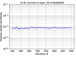
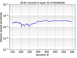
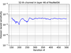
Figure 3: The convergence of Hessian-based sensitivity throughout the Hutchinson iterations, for different channels of ResNet56. Here, the x-axis is the Hutchinson iteration, and the y-axis is the approximation for the sensitivity corresponding to Eq. 6. As one can see, the approximation converges after about 300 iterations.

Appendix D Limitations and Future Work

We believe it is critical for every work to clearly state its limitations, especially in this area. An important limitation is that computing the second order information adds some computational overhead. However, the overhead is actually much lower than expected as shown in Table 7. Another limitation is that in this work we only focused on computer vision (image classification) and natural language understanding, but it would be interesting to see how HAP would perform for more complex tasks such as object detection and machine translation. Third, in this paper, we solely work on static pruning (i.e., the model is fixed after pruning). However, for different inputs, the model can be adaptively/dynamically pruned so that we can minimize the accuracy degradation. We leave this as a future work.

Appendix E Additional Results

Here, we show the distribution of pruning for different channels of WideResNet32, ResNet56, and PreResNet29. See Figure 4. As one can see, HAP only prunes insensitive channels, and keeps channels with high sensitivity (computed based on Eq. 6).

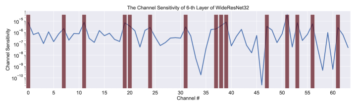
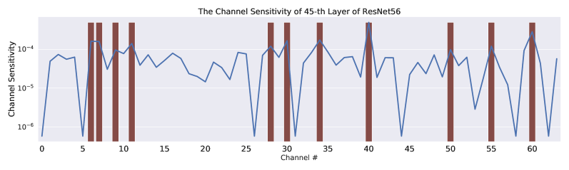
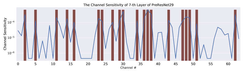
Figure 4: Illustration of sensitivity of the t6h layer of WideResNet32, 45th convolution layer of ResNet56, and the 7th convolution layer of PreResNet29. The x-axis denotes the channel index, and the blue line denotes the corresponding second-order sensitivity computed using Eq. 6. The red bar is added to channels that remain unpruned with the HAP method. As one can see, these correspond to sensitive channels that have large values on the blue line.

Table 7: Calculation time for channel wise sensitivity in HAP.

Method	WideResNet32	ResNet56	PreResNet
HAP	120s	61s	81s

References

- [1] https://github.com/neuripssubmission5022/hessianawarepruning, May 2021.
- [2] Haim Avron and Sivan Toledo. Randomized algorithms for estimating the trace of an implicit symmetric positive semi-definite matrix. Journal of the ACM (JACM), 58(2):8, 2011.
- [3] Zhaojun Bai, Gark Fahey, and Gene Golub. Some large-scale matrix computation problems. Journal of Computational and Applied Mathematics, 74(1-2):71–89, 1996.
- [4] Aydin Buluc and John R Gilbert. Challenges and advances in parallel sparse matrix-matrix multiplication. In 2008 37th International Conference on Parallel Processing, pages 503–510. IEEE, 2008.
- [5] Han Cai, Chuang Gan, Tianzhe Wang, Zhekai Zhang, and Song Han. Once-for-all: Train one network and specialize it for efficient deployment. arXiv preprint arXiv:1908.09791, 2019.
- [6] William B Dolan and Chris Brockett. Automatically constructing a corpus of sentential paraphrases. In Proceedings of the Third International Workshop on Paraphrasing (IWP2005), 2005.
- [7] Xin Dong, Shangyu Chen, and Sinno Pan. Learning to prune deep neural networks via layer-wise optimal brain surgeon. In Advances in Neural Information Processing Systems, pages 4857–4867, 2017.
- [8] Zhen Dong, Zhewei Yao, Daiyaan Arfeen, Amir Gholami, Michael W. Mahoney, and Kurt Keutzer. HAWQ-V2: Hessian aware trace-weighted quantization of neural networks. Advances in neural information processing systems, 2020.
- [9] Zhen Dong, Zhewei Yao, Amir Gholami, Michael W. Mahoney, and Kurt Keutzer. HAWQ: Hessian AWare Quantization of neural networks with mixed-precision. In The IEEE International Conference on Computer Vision (ICCV), October 2019.
- [10] Trevor Gale, Erich Elsen, and Sara Hooker. The state of sparsity in deep neural networks. arXiv preprint arXiv:1902.09574, 2019.
- [11] Amir Gholami, Kiseok Kwon, Bichen Wu, Zizheng Tai, Xiangyu Yue, Peter Jin, Sicheng Zhao, and Kurt Keutzer. SqueezeNext: Hardware-aware neural network design. Workshop paper in CVPR, 2018.
- [12] Luis Guerra, Bohan Zhuang, Ian Reid, and Tom Drummond. Automatic pruning for quantized neural networks. arXiv preprint arXiv:2002.00523, 2020.
- [13] Shaopeng Guo, Yujie Wang, Quanquan Li, and Junjie Yan. Dmcp: Differentiable markov channel pruning for neural networks. In Proceedings of the IEEE/CVF Conference on Computer Vision and Pattern Recognition, pages 1539–1547, 2020.
- [14] Ghouthi Boukli Hacene, Vincent Gripon, Matthieu Arzel, Nicolas Farrugia, and Yoshua Bengio. Quantized guided pruning for efficient hardware implementations of convolutional neural networks. arXiv preprint arXiv:1812.11337, 2018.
- [15] Song Han, Jeff Pool, John Tran, and William Dally. Learning both weights and connections for efficient neural network. In Advances in neural information processing systems, pages 1135–1143, 2015.
- [16] Babak Hassibi and David G Stork. Second order derivatives for network pruning: Optimal brain surgeon. In Advances in neural information processing systems, pages 164–171, 1993.
- [17] Babak Hassibi, David G Stork, and Gregory J Wolff. Optimal brain surgeon and general network pruning. In IEEE international conference on neural networks, pages 293–299. IEEE, 1993.
- [18] Yang He, Yuhang Ding, Ping Liu, Linchao Zhu, Hanwang Zhang, and Yi Yang. Learning filter pruning criteria for deep convolutional neural networks acceleration. In Proceedings of the IEEE/CVF Conference on Computer Vision and Pattern Recognition, pages 2009–2018, 2020.
- [19] Yihui He, Ji Lin, Zhijian Liu, Hanrui Wang, Li-Jia Li, and Song Han. Amc: Automl for model compression and acceleration on mobile devices. In Proceedings of the European Conference on Computer Vision (ECCV), pages 784–800, 2018.
- [20] Yang He, Ping Liu, Ziwei Wang, Zhilan Hu, and Yi Yang. Filter pruning via geometric median for deep convolutional neural networks acceleration. In Proceedings of the IEEE Conference on Computer Vision and Pattern Recognition, pages 4340–4349, 2019.
- [21] Yihui He, Xiangyu Zhang, and Jian Sun. Channel pruning for accelerating very deep neural networks. In Proceedings of the IEEE International Conference on Computer Vision, pages 1389–1397, 2017.
- [22] Geoffrey Hinton, Oriol Vinyals, and Jeff Dean. Distilling the knowledge in a neural network. Workshop paper in NIPS, 2014.
- [23] Andrew Howard, Mark Sandler, Grace Chu, Liang-Chieh Chen, Bo Chen, Mingxing Tan, Weijun Wang, Yukun Zhu, Ruoming Pang, Vijay Vasudevan, et al. Searching for mobilenetv3. In Proceedings of the IEEE International Conference on Computer Vision, pages 1314–1324, 2019.
- [24] Andrew G Howard, Menglong Zhu, Bo Chen, Dmitry Kalenichenko, Weijun Wang, Tobias Weyand, Marco Andreetto, and Hartwig Adam. Mobilenets: Efficient convolutional neural networks for mobile vision applications. arXiv preprint arXiv:1704.04861, 2017.
- [25] Zehao Huang and Naiyan Wang. Data-driven sparse structure selection for deep neural networks. In Proceedings of the European conference on computer vision (ECCV), pages 304–320, 2018.
- [26] Itay Hubara, Matthieu Courbariaux, Daniel Soudry, Ran El-Yaniv, and Yoshua Bengio. Quantized neural networks: Training neural networks with low precision weights and activations. The Journal of Machine Learning Research, 18(1):6869–6898, 2017.
- [27] Forrest N Iandola, Song Han, Matthew W Moskewicz, Khalid Ashraf, William J Dally, and Kurt Keutzer. SqueezeNet: AlexNet-level accuracy with 50x fewer parameters and¡ 0.5 mb model size. arXiv preprint arXiv:1602.07360, 2016.
- [28] Benoit Jacob, Skirmantas Kligys, Bo Chen, Menglong Zhu, Matthew Tang, Andrew Howard, Hartwig Adam, and Dmitry Kalenichenko. Quantization and training of neural networks for efficient integer-arithmetic-only inference. In Proceedings of the IEEE Conference on Computer Vision and Pattern Recognition, pages 2704–2713, 2018.
- [29] Raghuraman Krishnamoorthi. Quantizing deep convolutional networks for efficient inference: A whitepaper. arXiv preprint arXiv:1806.08342, 2018.
- [30] Alex Krizhevsky, Vinod Nair, and Geoffrey Hinton. Cifar-10 (canadian institute for advanced research). URL http://www. cs. toronto. edu/kriz/cifar. html, 5, 2010.
- [31] Alex Krizhevsky, Ilya Sutskever, and Geoffrey E Hinton. ImageNet classification with deep convolutional neural networks. In Advances in neural information processing systems, pages 1097–1105, 2012.
- [32] Se Jung Kwon, Dongsoo Lee, Byeongwook Kim, Parichay Kapoor, Baeseong Park, and Gu-Yeon Wei. Structured compression by weight encryption for unstructured pruning and quantization. In Proceedings of the IEEE/CVF Conference on Computer Vision and Pattern Recognition, pages 1909–1918, 2020.
- [33] Yann LeCun, John S Denker, and Sara A Solla. Optimal brain damage. In Advances in neural information processing systems, pages 598–605, 1990.
- [34] Namhoon Lee, Thalaiyasingam Ajanthan, and Philip HS Torr. Snip: Single-shot network pruning based on connection sensitivity. arXiv preprint arXiv:1810.02340, 2018.
- [35] Bailin Li, Bowen Wu, Jiang Su, and Guangrun Wang. Eagleeye: Fast sub-net evaluation for efficient neural network pruning. In European Conference on Computer Vision, pages 639–654. Springer, 2020.
- [36] Hao Li, Asim Kadav, Igor Durdanovic, Hanan Samet, and Hans Peter Graf. Pruning filters for efficient convnets. arXiv preprint arXiv:1608.08710, 2016.
- [37] Mingbao Lin, Rongrong Ji, Yan Wang, Yichen Zhang, Baochang Zhang, Yonghong Tian, and Ling Shao. Hrank: Filter pruning using high-rank feature map. In Proceedings of the IEEE/CVF Conference on Computer Vision and Pattern Recognition, pages 1529–1538, 2020.
- [38] Shaohui Lin, Rongrong Ji, Yuchao Li, Yongjian Wu, Feiyue Huang, and Baochang Zhang. Accelerating convolutional networks via global & dynamic filter pruning. In IJCAI, pages 2425–2432, 2018.
- [39] Shaohui Lin, Rongrong Ji, Chenqian Yan, Baochang Zhang, Liujuan Cao, Qixiang Ye, Feiyue Huang, and David Doermann. Towards optimal structured cnn pruning via generative adversarial learning. In Proceedings of the IEEE Conference on Computer Vision and Pattern Recognition, pages 2790–2799, 2019.
- [40] Yinhan Liu, Myle Ott, Naman Goyal, Jingfei Du, Mandar Joshi, Danqi Chen, Omer Levy, Mike Lewis, Luke Zettlemoyer, and Veselin Stoyanov. RoBERTa: A robustly optimized bert pretraining approach. arXiv preprint arXiv:1907.11692, 2019.
- [41] Zhuang Liu, Jianguo Li, Zhiqiang Shen, Gao Huang, Shoumeng Yan, and Changshui Zhang. Learning efficient convolutional networks through network slimming. In Proceedings of the IEEE International Conference on Computer Vision, pages 2736–2744, 2017.
- [42] Zechun Liu, Haoyuan Mu, Xiangyu Zhang, Zichao Guo, Xin Yang, Kwang-Ting Cheng, and Jian Sun. Metapruning: Meta learning for automatic neural network channel pruning. In Proceedings of the IEEE International Conference on Computer Vision, pages 3296–3305, 2019.
- [43] Zhuang Liu, Mingjie Sun, Tinghui Zhou, Gao Huang, and Trevor Darrell. Rethinking the value of network pruning. arXiv preprint arXiv:1810.05270, 2018.
- [44] Jian-Hao Luo, Jianxin Wu, and Weiyao Lin. Thinet: A filter level pruning method for deep neural network compression. In Proceedings of the IEEE international conference on computer vision, pages 5058–5066, 2017.
- [45] Li Lyna Zhang, Yuqing Yang, Yuhang Jiang, Wenwu Zhu, and Yunxin Liu. Fast hardware-aware neural architecture search. In Proceedings of the IEEE/CVF Conference on Computer Vision and Pattern Recognition Workshops, pages 692–693, 2020.
- [46] Ningning Ma, Xiangyu Zhang, Hai-Tao Zheng, and Jian Sun. Shufflenet v2: Practical guidelines for efficient cnn architecture design. In Proceedings of the European Conference on Computer Vision (ECCV), pages 116–131, 2018.
- [47] M. W. Mahoney. Randomized algorithms for matrices and data. Foundations and Trends in Machine Learning. NOW Publishers, Boston, 2011.
- [48] Huizi Mao, Song Han, Jeff Pool, Wenshuo Li, Xingyu Liu, Yu Wang, and William J Dally. Exploring the regularity of sparse structure in convolutional neural networks. Workshop paper in CVPR, 2017.
- [49] Paul Michel, Omer Levy, and Graham Neubig. Are sixteen heads really better than one? arXiv preprint arXiv:1905.10650, 2019.
- [50] Asit Mishra and Debbie Marr. Apprentice: Using knowledge distillation techniques to improve low-precision network accuracy. arXiv preprint arXiv:1711.05852, 2017.
- [51] Pavlo Molchanov, Stephen Tyree, Tero Karras, Timo Aila, and Jan Kautz. Pruning convolutional neural networks for resource efficient inference. arXiv preprint arXiv:1611.06440, 2016.
- [52] Sejun Park, Jaeho Lee, Sangwoo Mo, and Jinwoo Shin. Lookahead: a far-sighted alternative of magnitude-based pruning. arXiv preprint arXiv:2002.04809, 2020.
- [53] Antonio Polino, Razvan Pascanu, and Dan Alistarh. Model compression via distillation and quantization. arXiv preprint arXiv:1802.05668, 2018.
- [54] Pranav Rajpurkar, Jian Zhang, Konstantin Lopyrev, and Percy Liang. SQuAD: 100,000+ questions for machine comprehension of text. arXiv preprint arXiv:1606.05250, 2016.
- [55] Mark Sandler, Andrew Howard, Menglong Zhu, Andrey Zhmoginov, and Liang-Chieh Chen. MobileNetV2: Inverted residuals and linear bottlenecks. In Proceedings of the IEEE Conference on Computer Vision and Pattern Recognition, pages 4510–4520, 2018.
- [56] Mingxing Tan, Bo Chen, Ruoming Pang, Vijay Vasudevan, Mark Sandler, Andrew Howard, and Quoc V Le. Mnasnet: Platform-aware neural architecture search for mobile. In Proceedings of the IEEE Conference on Computer Vision and Pattern Recognition, pages 2820–2828, 2019.
- [57] Frederick Tung and Greg Mori. Clip-q: Deep network compression learning by in-parallel pruning-quantization. In Proceedings of the IEEE Conference on Computer Vision and Pattern Recognition, pages 7873–7882, 2018.
- [58] Ashish Vaswani, Noam Shazeer, Niki Parmar, Jakob Uszkoreit, Llion Jones, Aidan N Gomez, Łukasz Kaiser, and Illia Polosukhin. Attention is all you need. In Advances in neural information processing systems, pages 5998–6008, 2017.
- [59] Alex Wang, Amanpreet Singh, Julian Michael, Felix Hill, Omer Levy, and Samuel R Bowman. GLUE: A multi-task benchmark and analysis platform for natural language understanding. arXiv preprint arXiv:1804.07461, 2018.
- [60] Chaoqi Wang, Roger Grosse, Sanja Fidler, and Guodong Zhang. Eigendamage: Structured pruning in the kronecker-factored eigenbasis. arXiv preprint arXiv:1905.05934, 2019.
- [61] Ying Wang, Yadong Lu, and Tijmen Blankevoort. Differentiable joint pruning and quantization for hardware efficiency. In European Conference on Computer Vision, pages 259–277. Springer, 2020.
- [62] Bichen Wu, Xiaoliang Dai, Peizhao Zhang, Yanghan Wang, Fei Sun, Yiming Wu, Yuandong Tian, Peter Vajda, Yangqing Jia, and Kurt Keutzer. FBNet: Hardware-aware efficient convnet design via differentiable neural architecture search. In Proceedings of the IEEE Conference on Computer Vision and Pattern Recognition, pages 10734–10742, 2019.
- [63] Jiaxiang Wu, Cong Leng, Yuhang Wang, Qinghao Hu, and Jian Cheng. Quantized convolutional neural networks for mobile devices. In Proceedings of the IEEE Conference on Computer Vision and Pattern Recognition, pages 4820–4828, 2016.
- [64] Xia Xiao, Zigeng Wang, and Sanguthevar Rajasekaran. Autoprune: Automatic network pruning by regularizing auxiliary parameters. In Advances in Neural Information Processing Systems, pages 13681–13691, 2019.
- [65] Tien-Ju Yang, Yu-Hsin Chen, and Vivienne Sze. Designing energy-efficient convolutional neural networks using energy-aware pruning. In Proceedings of the IEEE Conference on Computer Vision and Pattern Recognition, pages 5687–5695, 2017.
- [66] Tien-Ju Yang, Andrew Howard, Bo Chen, Xiao Zhang, Alec Go, Mark Sandler, Vivienne Sze, and Hartwig Adam. Netadapt: Platform-aware neural network adaptation for mobile applications. In Proceedings of the European Conference on Computer Vision (ECCV), pages 285–300, 2018.
- [67] Zhewei Yao, Amir Gholami, Kurt Keutzer, and Michael W. Mahoney. PyHessian: Neural networks through the lens of the Hessian. arXiv preprint arXiv:1912.07145, 2019.
- [68] Zhewei Yao, Amir Gholami, Sheng Shen, Kurt Keutzer, and Michael W Mahoney. Adahessian: An adaptive second order optimizer for machine learning. arXiv preprint arXiv:2006.00719, 2020.
- [69] Hongxu Yin, Pavlo Molchanov, Jose M Alvarez, Zhizhong Li, Arun Mallya, Derek Hoiem, Niraj K Jha, and Jan Kautz. Dreaming to distill: Data-free knowledge transfer via deepinversion. In Proceedings of the IEEE/CVF Conference on Computer Vision and Pattern Recognition, pages 8715–8724, 2020.
- [70] Ruichi Yu, Ang Li, Chun-Fu Chen, Jui-Hsin Lai, Vlad I Morariu, Xintong Han, Mingfei Gao, Ching-Yung Lin, and Larry S Davis. Nisp: Pruning networks using neuron importance score propagation. In Proceedings of the IEEE Conference on Computer Vision and Pattern Recognition, pages 9194–9203, 2018.
- [71] Wenyuan Zeng and Raquel Urtasun. Mlprune: Multi-layer pruning for automated neural network compression. 2018.
- [72] Xiangyu Zhang, Xinyu Zhou, Mengxiao Lin, and Jian Sun. Shufflenet: An extremely efficient convolutional neural network for mobile devices. In Proceedings of the IEEE Conference on Computer Vision and Pattern Recognition, pages 6848–6856, 2018.
- [73] Chenglong Zhao, Bingbing Ni, Jian Zhang, Qiwei Zhao, Wenjun Zhang, and Qi Tian. Variational convolutional neural network pruning. In Proceedings of the IEEE Conference on Computer Vision and Pattern Recognition, pages 2780–2789, 2019.
- [74] Michael Zhu and Suyog Gupta. To prune, or not to prune: exploring the efficacy of pruning for model compression. arXiv preprint arXiv:1710.01878, 2017.
- [75] Zhuangwei Zhuang, Mingkui Tan, Bohan Zhuang, Jing Liu, Yong Guo, Qingyao Wu, Junzhou Huang, and Jinhui Zhu. Discrimination-aware channel pruning for deep neural networks. In Advances in Neural Information Processing Systems, pages 875–886, 2018.