Inferring solar differential rotation through normal-mode coupling using Bayesian statistics

Abstract

Normal-mode helioseismic data analysis uses observed solar oscillation spectra to infer perturbations in the solar interior due to global and local-scale flows and structural asphericity. Differential rotation, the dominant global-scale axisymmetric perturbation, has been tightly constrained primarily using measurements of frequency splittings via “$a$-coefficients”. However, the frequency-splitting formalism invokes the approximation that multiplets are isolated. This assumption is inaccurate for modes at high angular degrees. Analysing eigenfunction corrections, which respect cross coupling of modes across multiplets, is a more accurate approach. However, applying standard inversion techniques using these cross-spectral measurements yields $a$-coefficients with a significantly wider spread than the well-constrained results from frequency splittings. In this study, we apply Bayesian statistics to infer $a$-coefficients due to differential rotation from cross spectra for both $f$-modes and $p$-modes. We demonstrate that this technique works reasonably well for modes with angular degrees $\ell=50-291$. The inferred $a_{3}-$coefficients are found to be within $1$ nHz of the frequency splitting values for $\ell>200$. We also show that the technique fails at $\ell<50$ owing to the insensitivity of the measurement to the perturbation. These results serve to further establish mode coupling as an important helioseismic technique with which to infer internal structure and dynamics, both axisymmetric (e.g., meridional circulation) and non-axisymmetric perturbations.

1 Introduction

The strength and variation of observed solar activity is governed by the spatio-temporal dependence of flow fields in the convective envelope (Charbonneau, 2005; Fan, 2009). Thus, understanding the physics that governs the evolution and sustenance of the activity cycle of the Sun necessitates imaging its internal layers. While differential rotation has the most significant imprint on Dopplergram images (Schou et al., 1998), signatures due to weaker effects, such as meridional circulation (Giles et al., 1997; Basu et al., 1999; Zhao & Kosovichev, 2004; Gizon et al., 2020) and magnetic fields (Gough, 1990; Dziembowski & Goode, 2004; Antia et al., 2013), are also noticeable. The ability to image these weaker effects therefore critically depends on an accurate measurement of the dominant flows. This makes inferring the strength of the dominant flows along with assigning appropriate statistical uncertainties an important area of study.

Differences between normal modes of the Sun and those predicted using standard solar models may be used to constrain solar internal properties. The standard models are typically adiabatic, hydrodynamic, spherically symmetric and non-rotating, also referred to as SNRNMAIS (Lavely & Ritzwoller, 1992; Christensen-Dalsgaard et al., 1996). The usual labelling convention, using 3 quantum numbers, $(n,\ell,m)$, where $n$ denotes radial order, $\ell$ the angular degree, and $m$ the azimuthal order, are used to uniquely identify normal modes. Departures of solar structure from the SNRNMAIS are modelled as small perturbations (Christensen–Dalsgaard, 2003), which ultimately manifest themselves as observable shifts (or splittings) in the eigenfrequencies and distortions in the eigenfunctions (Woodard, 1989). The distorted eigenfunctions may be expressed as a linear combination of reference eigenfunctions and are said to be coupled with respect to the reference. Observed cross-spectra of spherical-harmonic time series corresponding to full-disk Dopplergrams are used to measure eigenfunction distortion. In the present study, we use observational data from the Helioseismic Magnetic Imager (HMI) onboard the Solar Dynamics Observatory (Schou et al., 2012).

Different latitudes of the Sun rotate at different angular velocities, with the equator rotating faster than the poles (Howard et al., 1984; Ulrich et al., 1988). To an observer in a frame co-rotating at a specific rotation rate $\bar{\Omega}$ of the Sun, this latitudinal rotational shear is the most significant perturbation to the reference model. This large-scale toroidal flow $\Omega\,(r,\theta)$ is well approximated as being time-independent (shown to vary less than 5% over the last century in Gilman, 1974; Howard et al., 1984; Basu & Antia, 2003) and zonal, with variations only along the radius $r$ and co-latitude $\theta$.

Very low $\ell\leq 5$ modes penetrate the deepest layers of the Sun and were used in earlier attempts to constrain the rotation rate in the core and radiative interior (Claverie et al., 1981; Chaplin et al., 1999; Eff-Darwich et al., 2002; Couvidat et al., 2003; Chaplin et al., 2004). However, observed solar activity is believed to be governed by the coupling of differential rotation and magnetic fields in the bulk of the convection zone (Miesch, 2005). Subsequently, studies using intermediate $\ell\leq 100$ (Duvall & Harvey, 1984; Brown & Morrow, 1987; Brown et al., 1989; Libbrecht, 1989; Duvall et al., 1996) and modes with relatively high $\ell\leq 250$ (Thompson et al., 1996; Kosovichev et al., 1997; Schou et al., 1998) yielded overall convergent results for the rotation profile. Among other features of the convection zone (Howe, 2009), these studies established the presence of shear layers at the base of the convection zone (the tachocline) and below the solar surface.

Most of these studies used measurements of frequency splittings in a condensed convention known as $a$-coefficients (Ritzwoller & Lavely, 1991). The azimuthal and temporal independence make differential rotation particularly amenable to inversion via $a$-coefficients. The assumption behind this formalism is that multiplets, identified by  $(n,\ell)$, are well separated in frequency from each other, known as the ‘isolated multiplet approximation’. This assumption holds true when differential rotation is the sole perturbation under consideration (Lavely & Ritzwoller, 1992), even at considerably high $\ell$. We therefore state at the outset that estimates of $a$-coefficients determined from frequency splitting serve as reliable measures of differential rotation (Chatterjee & Antia, 2009). Nevertheless, the estimation of non-axisymmetric perturbations requires a rigorous treatment honoring the cross coupling of multiplets (Hanasoge et al., 2017; Das et al., 2020). In such cases, measuring changes to the eigenfunctions is far more effective than, for instance, the $a$-coefficient formalism. As a first step, it is therefore important to explore the potential of eigenfunction corrections to infer differential rotation.

The theoretical modeling of eigenfunction corrections for given axisymmetric – zonal and meridional – flow fields may be traced back to Woodard (1989), followed up by further investigations Woodard (2000); Gough & Hindman (2010); Vorontsov (2007); Schad et al. (2011). Schad et al. (2013) and Schad & Roth (2020) used observables in the form of mode-amplitude ratios to infer meridional circulation and differential rotation, respectively. In this study, we adopt the closed-form analytical expression for correction coefficients first proposed by Vorontsov (2007) and subsequently verified to be accurate up to angular degrees as high as $\ell\leq 1000$ Vorontsov (2011), henceforth V11. The method of using cross-spectral signals to fit eigenfunction corrections was first applied by Woodard et al. (2013), henceforth W13, to infer differential rotation and meridional circulation. A simple least-squares fitting, assuming a unit covariance matrix, was used for inversions in W13. Their results of odd $a$-coefficients (which encodes differential rotation), even though qualitatively similar, show a considerably larger spread than the results from frequency splittings. Moreover, the authors of W13 note that the inferred meridional flow was “less satisfactory” [than their zonal flow estimates]. Cross spectra are dominated by differential rotation, a much larger perturbation than meridional circulation. Although zonal and meridional flows are measured in different cross-spectral channels, the inference of meridional flow is affected by differential rotation through leakage. Thus, the accurate determination of odd $a$-coefficients is critical to the inference of meridional flow. The relatively large spread in inferences of differential rotation obtained by W13 may be due to (a) a poorly conditioned minimizing function with multiple local minima surrounding the expected (frequency splitting) minima, (b) a relative insensitivity of various modes to differential rotation, resulting in a flat minimizing function close to the expected minima, (c) an inaccurate estimation of the minimizing function on account of assuming a unit-data covariance matrix, and/or (d) eigenfunction corrections only yielding accurate results in the limit of large $\ell$ ($>250$), where the isolated-multiplet approximation starts worsening.

In this study, we investigate the above issues and explore the potential of using eigenfunction corrections as a means to infer differential rotation using tools from Bayesian statistics. We apply the Markov Chain Monte Carlo (MCMC) algorithm (Metropolis & Ulam, 1949; Metropolis et al., 1953) using a minimizing function calculated in the L2 norm, adequately weighted by data variance. We do not bias the MCMC sampler in light of any previous measurement, effectively using an uninformed prior. The results inferred, therefore, are an independent measurement constrained only by observed cross spectra. Since Bayesian inference is a probabilistic approach to parameter estimation, we obtain joint probability-density functions in the $a$-coefficient space. This allows us to rigorously compute uncertainties associated with the measurements. We compare and qualify the results obtained with independent measurements from frequency splitting and those obtained using similar cross-spectral analysis in W13. Further, we report the inadequacy of this method for low angular-degree modes on account of poor sensitivity of spectra to rotation via $a$-coefficients.

The structure of this paper is as follows. We establish mathematical notations and describe the basic physics of normal-mode helioseismology in Section 2.1. The governing equations which we use for modeling cross spectra using eigenfunction-correction coefficients are outlined in Section 2.2. Section 3 elaborates the steps for computing the observed cross spectra and building the misfit function and estimating data variance for performing the MCMC. Results are discussed in Section 4. Using the $a$-coefficients inferred from MCMC, cross-spectra are reconstructed in Section 4.1. A discussion on sensitivity of the current model to the model parameters is presented in Section 4.2. The conclusions from this work are reported in Section 5.

2 Theoretical Formulation

2.1 Basic Framework and Notation

For inferring flow profiles in the solar interior, we begin by considering the system of coupled hydrodynamic equations, namely,

$$\partial_{t}\rho = -\bm{\nabla}\cdot(\rho\,\mathbf{v}),$$ (1)

$$\rho(\partial_{t}\mathbf{v}+\mathbf{v}\cdot\bm{\nabla}\mathbf{v}) = -\bm{\nabla}P-\rho\bm{\nabla}\phi,$$ (2)

$$\partial_{t}P = -\mathbf{v}\cdot\bm{\nabla}P-\gamma\,P\,\bm{\nabla}\cdot\mathbf{v},$$ (3)

where $\rho$ is the mass density, $\mathbf{v}$ the material velocity, $P$ the pressure, $\phi$ the gravitational potential and $\gamma$ the ratio of specific heats determined by an adiabatic equation of state. The eigenstates of the Sun are modeled as linear combinations of the eigenstates of a standard solar model. Here we use model S as this reference state, which is discussed in Christensen-Dalsgaard et al. (1996). In absence of background flows, $\tilde{{\mathbf{v}}}={\bf 0}$, the zeroth-order hydrodynamic equations trivially reduce to the hydrostatic equilibrium $\bm{\nabla}\tilde{P}+\tilde{\rho}\bm{\nabla}\tilde{\phi}=0$. Hereafter, all zeroth-order static fields, unperturbed mode eigenfrequencies, eigenfunctions and amplitudes corresponding to the reference model will be indicated using tilde (to maintain consistency with notation used in W13). In response to small perturbations to the static reference model, the system exhibits oscillations $\mbox{\boldmath$\bf\xi$}(\mathbf{r},t)$. These oscillations may be decomposed into resonant “normal modes” of the system, labeled by index $k$, with characteristic frequency $\tilde{\omega}_{k}$ and spatial pattern $\tilde{}\mbox{\boldmath$\bf\xi$}_{k}$, as follows:

$$\bm{\xi}(\bm{r},t)=\sum_{k}\tilde{\Lambda}_{k}(t)\,\tilde{\bm{\xi}}_{k}(\bm{r})\exp(i\tilde{\omega}_{k}t),$$ (4)

where $\tilde{\Lambda}_{k}$ are the respective mode amplitudes and $\bm{r}=(r,\theta,\phi)$ denote spherical-polar coordinates. Linearizing eqns. (1)–(3) about the hydrostatic background model gives (for a detailed derivation refer to Christensen–Dalsgaard, 2003)

$$\mathcal{L}_{0}\tilde{\bm{\xi}}_{k}=-\bm{\nabla}(\tilde{\rho}c_{s}^{2}\,\bm{\nabla}\cdot\tilde{\bm{\xi}}_{k}-\tilde{\rho}g\,\tilde{\bm{\xi}}_{k}\cdot\hat{\bm{e}}_{r})-g\,\hat{\bm{e}}_{r}\bm{\nabla}\cdot(\tilde{\rho}\,\tilde{\bm{\xi}}_{k})=\tilde{\rho}\,\tilde{\omega}_{k}^{2}\,\tilde{\bm{\xi}_{k}}.$$ (5)

Here $\tilde{\rho}(r),c_{s}(r)$, and $g(r)$ denote density, sound speed, and gravity (directed radially inward) respectively of the reference solar model, and $\mathcal{L}\,_{0}$ is the self-adjoint unperturbed wave operator. This ensures that the eigenfrequencies $\tilde{\omega}_{k}$ are real and eigenfunctions $\tilde{\mbox{\boldmath$\bf\xi$}}_{k}$ are orthogonal. Introducing flows and other structure perturbations through the operator $\delta\mathcal{L}\,$ (e.g., magnetic fields or ellipticity) modifies the unperturbed wave equation (5) to

$$\tilde{\rho}\,\omega_{k}^{2}\,\bm{\xi}_{k}=\left(\mathcal{L}\,_{0}+\delta\mathcal{L}\,\right)\bm{\xi}_{k},$$ (6)

where $\omega_{k}=\tilde{\omega}_{k}+\delta\omega_{k}$ and $\mbox{\boldmath$\bf\xi$}_{k}=\sum_{k^{\prime}}c_{k^{\prime}}\tilde{\mbox{\boldmath$\bf\xi$}}_{k^{\prime}}$ are the eigenfrequency and eigenfunction associated with the perturbed wave operator $\mathcal{L}\,_{0}+\delta\mathcal{L}\,$. The Sun, a predominantly hydrodynamic system, is thus treated as a fluid body with vanishing shear modulus (Dahlen & Tromp, 1998). This is unfavourable for sustaining shear waves and therefore the eigenfunctions of the reference model are very well approximated as spheroidal (Chandrasekhar & Kendall, 1957),

$$\tilde{\bm{\xi}}_{k}(r,\theta,\phi)={}_{n}U{}_{\ell}(r)\,Y_{\ell m}(\theta,\phi)\,\hat{\bm{e}}_{r}+{}_{n}V{}_{\ell}(r)\,\bm{\nabla}_{1}Y_{\ell m}(\theta,\phi).$$ (7)

$\bm{\bm{\nabla}}_{1}=\hat{\bm{e}}_{\theta}\,\partial_{\theta}+\hat{\bm{e}}_{\phi}\,(\sin\theta)^{-1}\partial_{\phi}$ is the dimensionless lateral covariant derivative operator. Suitably normalized eigenfunctions $\tilde{\mbox{\boldmath$\bf\xi$}}_{k}$ and $\tilde{\mbox{\boldmath$\bf\xi$}}_{k^{\prime}}$, where $k^{\prime}=(n^{\prime},\ell^{\prime},m^{\prime})$, satisfy the orthonormality condition

$$\int_{\odot}\mathrm{d}^{3}\mathbf{r}\,\rho\,\bm{\tilde{\xi}}_{k^{\prime}}^{*}\cdot\bm{\tilde{\xi}}_{k}=\delta_{n^{\prime}n}\,\delta_{\ell^{\prime}\ell}\,\delta_{m^{\prime}m}.$$ (8)

Since we observe only half the solar surface, orthogonality cannot be used to extract each mode separately. Windowing in the spatial domain results in spectral broadening, where contributions from neighbouring modes seep into the observed mode signal $\varphi^{\ell m}(\omega)$, as described by the leakage matrix (Schou & Brown, 1994),

$$\varphi^{\ell m}(\omega)=\sum_{k^{\prime}}L^{\ell m}_{k^{\prime}}\,\Lambda^{k^{\prime}}(\omega)=\sum_{k^{\prime}}\tilde{L}^{\ell m}_{k^{\prime}}\,\ \tilde{\Lambda}^{k^{\prime}}(\omega).$$ (9)

Here, leakage matrices $L^{\ell m}_{k^{\prime}},\tilde{L}^{\ell m}_{k^{\prime}}$ and amplitudes $\Lambda^{k^{\prime}}(\omega),\tilde{\Lambda}^{k^{\prime}}(\omega)$ of the observed surface velocity field ${\mathbf{v}}(\omega)$ correspond to the bases of perturbed ($\mbox{\boldmath$\bf\xi$}_{k^{\prime}}$) and unperturbed eigenfunctions ($\tilde{\mbox{\boldmath$\bf\xi$}}_{k^{\prime}}$), respectively,

$${\mathbf{v}}=\sum_{k^{\prime}}\Lambda^{k^{\prime}}\mbox{\boldmath$\bf\xi$}_{k^{\prime}}=\sum_{k^{\prime}}\tilde{\Lambda}^{k^{\prime}}\tilde{\mbox{\boldmath$\bf\xi$}}_{k^{\prime}}.$$ (10)

Since leakage falls rapidly with increasing spectral distance $(|\ell-\ell^{\prime}|,|m-m^{\prime}|)$, Eqn. (9) demonstrates the entangling of modes in spectral proximity to $(\ell,m)$. The presence of a zeroth-order flow field $\tilde{{\mathbf{v}}}$ in Eqns. (1)–(3) gives rise to perturbed eigenfunctions $\mbox{\boldmath$\bf\xi$}_{k}$ and therefore introduces correction factors $c_{k}^{k^{\prime}}$ with respect to the unperturbed eigenfunctions $\tilde{\mbox{\boldmath$\bf\xi$}}_{k^{\prime}}$.

$$\mbox{\boldmath$\bf\xi$}_{k}=\sum_{k^{\prime}}c_{k}^{k^{\prime}}\tilde{\mbox{\boldmath$\bf\xi$}}_{k^{\prime}}.$$ (11)

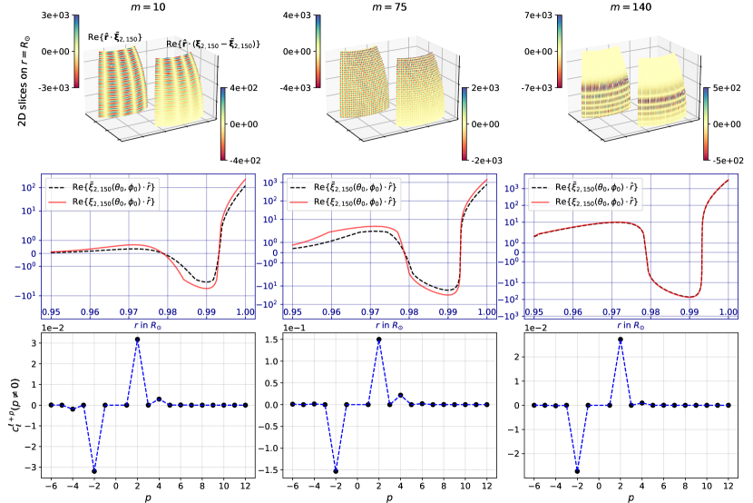
Figure 1: Differential rotation induces 3D distortions in radial eigenfunction of unperturbed mode $(n,l)=(2,150)$ for $m=10,75,140$ at radii $r/R_{\odot}=0.95,1.0$. Each column in the upper panel correspond to 2D surfaces for the undistorted eigenfunctions $\tilde{\bm{\xi}}_{nlm}$ in the left slice and differences between distorted and undistorted eigenfunctions $\hat{r}\cdot(\bm{\xi}_{nlm}-\tilde{\bm{\xi}}_{nlm})$ in the right slice. The middle panel shows the difference in the radial variation of eigenfunctions for a chosen $(\theta_{0},\phi_{0})=(67.8^{\circ},177.6^{\circ})$. The lower panels indicate the magnitudes of the coupling coefficients that induce eigenfunction distortion, as in Eqn. (11). The self-coupling coefficients $c^{\ell m}_{\ell m}$ (i.e., $p=0$), being the most dominant, are not shown, in order to highlight the contributions of cross-coupling coefficients ($p\neq 0$.)

Using this, the statistical expectation of the cross-spectral measurement is expressed as in Eqns. (14)–(17) of W13,

$$\langle\varphi^{\ell^{\prime}m^{\prime}}\varphi^{\ell m}\rangle=\sum_{i,j,k}\tilde{L}^{\ell^{\prime}m^{\prime}}_{j}\,\tilde{L}^{\ell m*}_{k}\,c^{j}_{i}\,c^{k*}_{i}\,\langle|\Lambda^{i}(\omega)|^{2}\rangle,$$ (12)

where $\langle|\Lambda^{i}(\omega)|^{2}\rangle$ denotes Lorentzians centered at resonant frequencies $\omega=\omega_{i}$ corresponding to the perturbed modes $\mbox{\boldmath$\bf\xi$}_{i}$.

2.2 Eigenfunction corrections due to axisymmetric flows

This study uses the fact that eigenfunction-correction factors $c_{k}^{k^{\prime}}$ in Eqn. (11) carry information about the flow field $\tilde{{\mathbf{v}}}$. Although this problem was first addressed by Woodard (1989), a rigorous treatment using perturbative analysis of mode coupling was only presented in V11. In this section, we outline the governing equations for the eigenfunction-correction factors $c_{k}^{k^{\prime}}$ due to differential rotation and meridional circulation as shown in V11. Upon introducing flows, the model-S eigenfunctions are corrected as follows:

$$\mbox{\boldmath$\bf\xi$}_{\ell}=\sum_{\ell^{\prime}}c_{\ell}^{\ell^{\prime}}\,\tilde{\mbox{\boldmath$\bf\xi$}}_{\ell^{\prime}}+\delta\mbox{\boldmath$\bf\xi$}_{\ell}=\sum_{p=0,\pm 1,\pm 2,...}c_{\ell}^{\ell+p}\,\tilde{\mbox{\boldmath$\bf\xi$}}_{\ell+p}+\delta\mbox{\boldmath$\bf\xi$}_{\ell},$$ (13)

where $p=\ell^{\prime}-\ell$ is used to label the offset (in angular degrees) of the neighbouring mode contributing to the distortion of the erstwhile unperturbed eigenfunction $\mbox{\boldmath$\bf\xi$}_{\ell}$ — visual illustration may be found in Figure 1. Correction factors $c_{\ell}^{\ell+p}$ solely from modes with the same radial orders and azimuthal degrees are considered in Eqn. (13) and therefore labels $n$ and $m$ are suppressed. $c_{\ell,m}^{\ell+p,m^{\prime}}=0$ for $m\neq m^{\prime}$ since differential rotation and meridional circulation are axisymmetric (see selection rules imposed due to Wigner 3-$j$ symbols in Appendix A of V11). Corrections from modes belonging to a different radial order $n$ are accumulated in $\delta\mbox{\boldmath$\bf\xi$}$. Following V11 and W13, subsequent treatment ignores terms in $\delta\mbox{\boldmath$\bf\xi$}$ since it is considered to be of the order of the perturbation $\delta\mathcal{L}\,$ or smaller (rendering them at least second order in perturbed quantities). This is because the correction factor $c_{n\ell}^{n^{\prime}\ell^{\prime}}$ is non-trivial only if modes ${}_{n}\mathrm{S}_{\ell}\,$ and ${}_{n^{\prime}}\mathrm{S}_{\ell^{\prime}}\,$ are proximal in frequency space as well as the angular degree $s$ of the perturbing flow satisfies the relation $|\ell^{\prime}-\ell|\leq s$. For modes belonging to different dispersion branches $(n\neq n^{\prime})$, with either $\ell$ or $\ell^{\prime}$ being moderately large ($>50$) the prior conditions are not satisfied, since, for differential rotation, the largest non-negligible angular degree of perturbation is $s=5$.

As shown in V11, using eigenfunction perturbations as in Eqn. (13) and eigenfrequency perturbations $\omega_{\ell}=\tilde{\omega}_{\ell}+\delta\omega_{\ell}$, the wave equation (6) reduces to an eigenvalue problem of the form

$$\mathbf{Z}\,\bm{\mathcal{C}}_{\ell}=\delta\omega_{\ell}\,\bm{\mathcal{C}}_{\ell},$$ (14)

where $\bm{\mathcal{C}}_{\ell}=\{...,c_{\ell}^{\ell-1},c_{\ell}^{\ell},c_{\ell}^{\ell+1},...\}$ are eigenvectors corresponding to the $(P\times P)$ self-adjoint matrix ${\mathbf{Z}}$ and $P=\mathrm{max}(|\ell^{\prime}-\ell|)$ denotes the largest offset of a contributing mode $\ell^{\prime}$ from $\ell$ according as Eqn. (13). From detailed considerations of first- and second-order quasi-degenerate perturbation theory, V11 showed that the following closed-form expression for correction coefficients is accurate up to angular degrees as high as $\ell=1000$:

$$c_{\ell}^{\ell+p}=\tfrac{1}{\pi}\int_{0}^{\pi}\cos\left[pt-\sum_{k=1,2,...}\tfrac{2}{k}\mathrm{Re}(b_{k})\sin{(kt)}\right]\times\mathrm{exp}\left[i\sum_{k=1,2,...}\tfrac{2}{k}\mathrm{Im}(b_{k})\cos{(kt)}\right]\mathrm{d}t,\qquad p=0,\pm 1,...,$$ (15)

where the convenient expressions for real and imaginary parts of $b_{k}$ are

$$\mathrm{Re}(b_{k}) = \ell\left(\frac{\partial\tilde{\omega}}{\partial\ell}\right)^{-1}_{n}\sum_{s+k=\mathrm{odd}}(-1)^{\frac{s-k+1}{2}}\frac{(s-k)!!(s+k)!!}{(s+k)!}\times P_{s}^{k}\left(\frac{m}{\ell}\right)\langle\Omega_{s}\rangle_{n\ell},\quad k=1,2,...$$ (16)

$$\mathrm{Im}(b_{k}) = k\ell\left(\frac{\partial\tilde{\omega}}{\partial\ell}\right)^{-1}_{n}\sum_{s+k=\mathrm{even}}(-1)^{\frac{s-k+2}{2}}\left(\frac{2s+1}{4\pi}\right)^{1/2}\frac{(s-k-1)!!(s+k-1)!!}{(s+k)!}\times P_{s}^{k}\left(\frac{m}{\ell}\right)\langle\frac{v_{s}}{r}\rangle_{n\ell},\quad k=1,2,....$$ (17)

We consider only odd-$s$ dependencies of $\Omega$. The even-$s$ correspond to North-South (NS) asymmetry in differential rotation and are estimated to be weak at the surface (NS asymmetry coefficients are estimated to be an order of magnitude smaller than their symmetric counterparts; Mdzinarishvili et al., 2020). The contribution of even-$s$ components to the real part of $b_{k}$ can thus be ignored. For the asymptotic limit of high-degrees,

$$\mathrm{Re}(b_{k})=\ell\left(\frac{\partial\tilde{\omega}}{\partial\ell}\right)_{n}^{-1}\sum_{s+k=odd}(-1)^{\frac{k-2}{2}}\frac{s!(s-k)!!(s+k)!!}{(s+k)!s!!s!!}\times a^{n\ell}_{s}\,P_{s}^{k}\left(\frac{m}{\ell}\right),\quad k=2,4,...,$$ (18)

$$a^{n\ell}_{s}\approx(-1)^{\frac{s-1}{2}}\frac{s!!s!!}{s!}\langle\Omega_{s}\rangle_{n\ell},\quad s=1,3,...$$ (19)

Figure 1 illustrates the distortion of eigenfunctions due to an equatorially symmetric differential rotation (using frequency splitting estimates of $a_{3}$ and $a_{5}$ coefficients). It can be seen that differences between distorted eigenfunctions $\bm{\xi}_{nlm}$ and their undistorted counterparts $\tilde{\bm{\xi}}_{nlm}$ are at around the $50\%$ level for some azimuthal orders. The correction coefficients, given by $c^{\ell+p,m}_{\ell,m}$, are shown in the bottom panel of Figure 1. Since the largest contribution to $\bm{\xi}_{\ell}$ comes from $\tilde{\bm{\xi}}_{\ell}$, $c^{\ell,m}_{\ell,m}(\gtrsim 0.8)$ are not plotted to highlight the corrections from neighbouring modes with $p\neq 0$. Visual inspection shows that $c^{\ell+p,m}_{\ell,m}$ have non-zero elements at $p=\pm 2,\pm 4$, as expected from selection rules due to the rotation field $\Omega_{s}(r)$ for $s=3,5$. High $\ell$ eigenfunctions are predominantly large close to the surface. Consequently, we see that their distortions are much larger at shallower than deeper depths. We choose to plot three cases — low, intermediate, and high $m$. For the extreme cases of $m=0$ and $m=\ell$, $c^{\ell+p,m}_{\ell,m}\sim 0$, since for odd $s$ and even $k$, $P_{s}^{k}(\mu)$ vanishes at $\mu=0,1$. Thus these eigenfunctions remain undistorted under an equatorially symmetric differential rotation.

For sake of completeness, it may be mentioned that the finite $c^{\ell+p,m}_{\ell,m}$ for $p\neq 0$ seemingly disqualifies the frequency-splitting measurements, which assume isolated multiplets — meaning $c^{\ell+p,m}_{\ell,m}=\delta_{p,0}$. However, it does not necessarily imply that the isolated multiplet approximation is poor at these angular degrees. If the eigenfunction error $\delta\bm{\xi}_{k}$ incurred on neglecting cross-coupling is of order $\mathcal{O}(\epsilon)$ then it can be shown (see Chapter 8 of Freidberg, 2014; Cutler, 2017) that the error in estimating eigenfrequency $\delta\omega_{k}$ is at most of order $\mathcal{O}(\epsilon^{2})$, where $\epsilon$ is small. To illustrate this further, if the error in estimating eigenfunction distortion on neglecting cross coupling $(p\neq 0)$ is written as $\epsilon\,\bm{\xi}_{\ell+p}$, then from inspecting Eqn. (13), we see that $\epsilon\sim|c_{\ell}^{\ell+p}|$. Upon investigating the $(n,\ell)=(2,150)$ case presented in Figure 1 for $p\neq 0$, we find $c_{\ell}^{\ell+p}\lesssim\mathcal{O}(10^{-1})$. The equivalent error incurred in eigenfrequency estimation may be computed according to the discussion in Section 4.4. This yields $\delta\omega/\omega\lesssim\mathcal{O}(10^{-2})$ in the range $150\leq\ell\leq 250$ thereby confirming the above argument for $\epsilon\sim 10^{-1}$. Given the leakage matrices and Lorentzians, the forward problem of modeling $\langle\varphi^{\ell^{\prime}m^{\prime}}\varphi^{\ell m*}\rangle$ requires constructing eigenfunction corrections $c^{\ell+p}_{\ell}$ using the $a$-coefficients in Eqn. (18) and the poloidal flow in Eqn. (17). Thus, for axisymmetric flows, the cross spectra for moderately large $\ell_{1}$ and $\ell_{2}$ from Eqn. (12) may be written more explicitly as

$$\langle\varphi^{\ell_{1},m_{1}}\,\varphi^{\ell_{2},m_{1}*}\rangle=\sum_{p,p^{\prime},\ell,m}\,\tilde{L}_{\ell+p,m}^{\ell_{1},m_{1}}\,\tilde{L}_{\ell+p^{\prime},m}^{\ell_{2},m_{2}}\,c_{\ell,m}^{\ell+p,m}\,c_{\ell,m}^{\ell+p^{\prime},m*}\,\langle|\Lambda^{\ell,m}(\omega)|^{2}\rangle.$$ (20)

The leakage matrices $\tilde{L}_{\ell+p,m}^{\ell_{1},m_{1}}$ impose bounds on the farthest modes that leak into mode amplitude $\varphi^{\ell m}$. This is because $\tilde{L}_{\ell+p,m}^{\ell_{1},m_{1}}$ is non-zero only when $\ell+p\in[\ell_{1}-\delta\ell,\ell_{1}+\delta\ell]$ and $m\in[m_{1}-\delta m,m_{1}+\delta m]$, where $\delta\ell$ and $\delta m$ are the farthest spectral offsets. Thus, for a given $\ell$, we must determine the correction coefficients $c_{\ell,m}^{\ell+p,m}$ such that $p\in[\ell_{1}-\delta\ell-\ell,\ell_{1}+\delta\ell-\ell]$. Similar bounds on $p^{\prime}$ in $c_{\ell,m}^{\ell+p^{\prime},m}$ are imposed by the second leakage matrix $\tilde{L}_{\ell+p^{\prime},m}^{\ell_{2},m_{2}}$, namely,

$$\langle\varphi^{\ell_{1},m_{1}}\,\varphi^{\ell_{1}+\Delta\ell,m_{1}*}\rangle=\sum_{p,p^{\prime},\ell,m}\,\tilde{L}_{\ell+p,m}^{\ell_{1},m_{1}}\,\tilde{L}_{\ell+p^{\prime},m}^{\ell_{1}+\Delta\ell,m_{1}}\,c_{\ell,m}^{\ell+p,m}\,c_{\ell,m}^{\ell+p^{\prime},m*}\,\langle|\Lambda^{\ell,m}(\omega)|^{2}\rangle.$$ (21)

Being significantly weaker than differential rotation, we neglect the contribution of meridional circulation (Imada & Fujiyama, 2018; Gizon et al., 2020) to the eigenfunction corrections.

3 Data Analysis

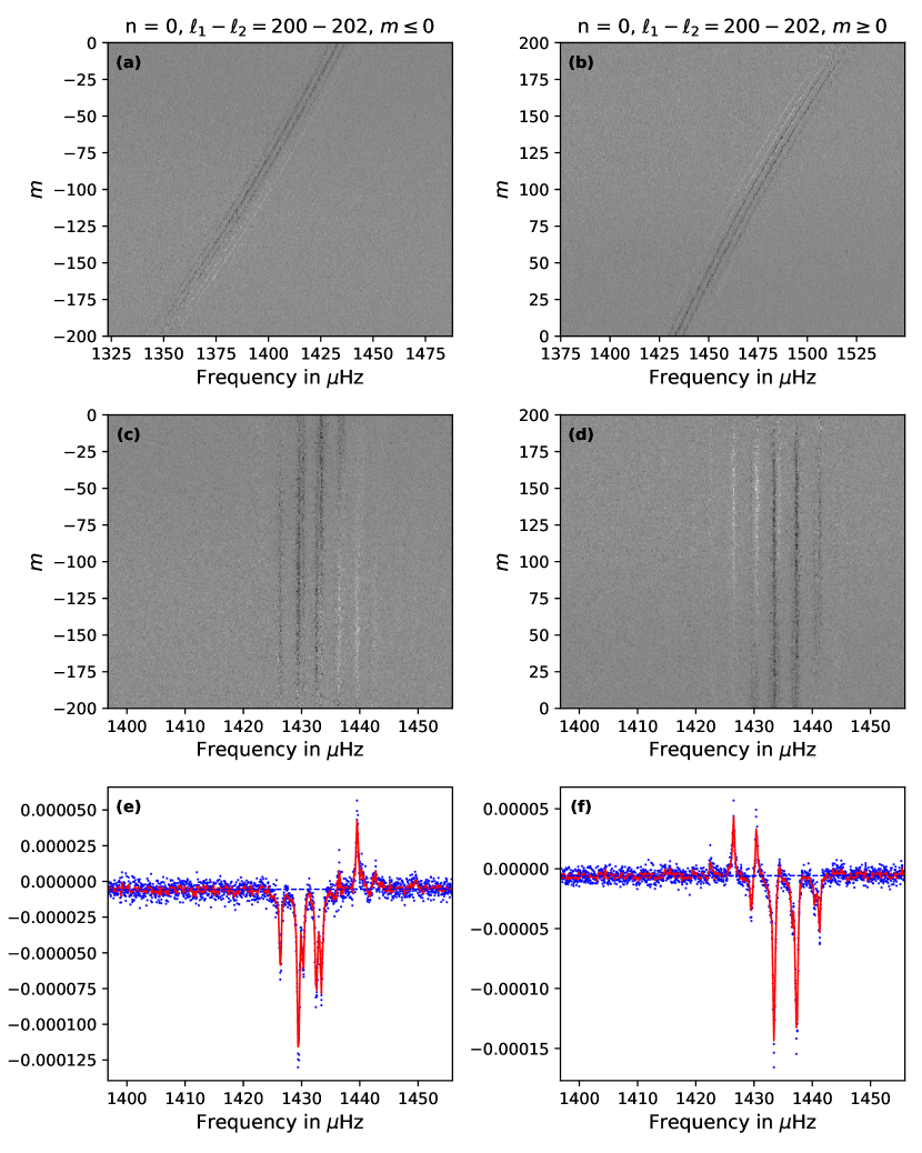
Figure 2: Cross-spectral signal for $\ell=200$, $\Delta\ell=2$ and $n=0$. Panel (a, b): Observed cross-spectrum corresponding to $m^{+}$ and $m^{-}$. Panel (c, d): Derotated cross spectrum corresponding to $m^{+}$ and $m^{-}$. Panel (e, f): $D^{\ell,\Delta\ell,\pm}_{n}$. The baseline is indicated by the dashed blue line. The blue dots represent observations from the five 72-day time series and the red curve corresponds to the expectation value of the cross-spectrum.

We use the full-disk 72-day gap-filled spherical-harmonic time series $\varphi^{\ell m}(t)$, which are recorded at a cadence of 45 seconds by HMI (Larson & Schou, 2015). The data are available for harmonic degrees in the range $\ell\leq 300$. The time series is transformed to the frequency domain to obtain $\varphi^{\ell m}(\omega)$. The negative-frequency components are associated with the negative $m$ components using the symmetry relation (Appendix A)

$$\varphi^{\ell,-|m|}(\omega)=(-1)^{|m|}\varphi^{\ell,|m|*}(-\omega).$$ (22)

The ensemble average of the cross spectrum is computed by averaging five continuous 72-day time series, which corresponds to 360 days of helioseismic data. The eigenfrequencies of the unperturbed model $\tilde{\omega}_{n\ell m}$ are degenerate in $m$, i.e., $\tilde{\omega}_{n\ell m}=\tilde{\omega}_{n\ell 0}$. Rotation breaks spherical symmetry and lifts the degeneracy in $m$. As in W13, we show the cross-spectrum for $n=0$ and $\ell=200$, $\Delta\ell=2$ in Figure 2. The effect of rotation is visible through the inclination of the ridges in the $m-\nu$ spectrum, as seen in Panels (a, b) of the figure. The multiple vertical ridges are due to leakage of power.

The cross spectra are derotated and stacked about the central frequency, corresponding to $m=0$, which is shown in Panels (c, d) of Figure 2. In order to improve the signal-to-noise ratio, the stacked cross spectrum is summed over azimuthal order $m$. This quantity is used to determine the extent of coupling, denoted by $D^{\ell,\Delta\ell,\pm}_{n}$. The $-$ ($+$) signs indicates summation over negative (positive) $m$. For notational convenience, we define $m^{+}$ when referring to $m\geq 0$ and $m^{-}$ to denote $m\leq 0$. The operation of stacking (derotating) the original spectra is denoted by $\mathcal{S}_{m}$. Since differential rotation affects only the real part of the cross-spectrum (see Eqn. 15), $D^{\ell,\Delta\ell,\pm}_{n}$ refers to the real part of the cross-spectrum.

$$D_{n}^{\ell,\Delta\ell,\pm}(\omega)=\left\langle\sum_{m^{\pm}}\mathcal{S}_{m}\left(\text{Re}\left[\varphi^{\ell m}(\omega)\varphi^{\ell+\Delta\ell,m*}(\omega)\right]\right)\right\rangle.$$ (23)

The cross-spectral model is a combination of Lorentzians and is based on Eqn. (21). The HMI-pipeline analysis provides us with mode amplitudes and linewidths for multiplets $(n,\ell)$. The $m$ dependence of frequency, $\omega_{n\ell m}-\omega_{nl0}$, is encoded in 36 frequency-splitting coefficients $(a^{nl}_{1},a^{nl}_{2},...,a^{nl}_{36})$. These values are used to construct the Lorentzians for the model, which is denoted by $M^{\ell,\Delta\ell,\pm}$ and expressed as

$$M^{\ell,\Delta\ell,\pm}_{n}(\omega)=\sum_{m\pm}\mathcal{S}_{m}\left(\sum_{p,p^{\prime},\ell,m^{\prime}}\,\tilde{L}_{\ell+p,m^{\prime}}^{\ell_{1},m}\,\tilde{L}_{\ell+p^{\prime},m^{\prime}}^{\ell_{1}+\Delta\ell,m}\,c_{\ell,m^{\prime}}^{\ell+p,m^{\prime}}\,c_{\ell,m^{\prime}}^{\ell+p^{\prime},m^{\prime}*}\,\langle|\Lambda^{\ell,m^{\prime}}_{n}(\omega)|^{2}\rangle\right).$$ (24)

As seen in Panels (e, f) of Figure 2, the cross spectra sit on a non-zero baseline. This is a non-seismic background and hence is explicitly fitted for before further analysis of the data. The complete model of the cross spectrum involves leakage from the power spectrum, eigenfunction coupling, as well as the non-seismic background, i.e., the data $D^{\ell,\Delta\ell,\pm}_{n}(\omega)$ is modelled as $M^{\ell,\Delta\ell,\pm}_{n}(\omega)+b^{\ell,\Delta\ell,\pm}_{n}(\omega)$. The baseline $b_{n}^{\ell,\Delta\ell,\pm}(\omega)$ is computed by considering 50 frequency bins on either side, far from resonance, and fitting a straight line through them, in a least-squares sense. The model $M^{\ell,\Delta\ell,\pm}_{n}(\omega)$ depends on the $a^{nl}_{3}$ and $a^{nl}_{5}$ splitting coefficients via the eigenfunction-correction coefficients $c^{\ell+p}_{\ell}$. A Bayesian-analysis approach is used to estimate the values $(a^{nl}_{3},a^{nl}_{5})$, using MCMC, described in Section 3.1. The misfit function that quantifies the goodness of a chosen model is given by

$$\Xi_{n}=\sum_{l,\omega,\pm}\left(\frac{D^{\ell,\Delta\ell,\pm}_{n}(\omega)-(M^{\ell,\Delta\ell,\pm}_{n}(\omega)+b^{\ell,\Delta\ell,\pm}_{n}(\omega))}{\sigma^{\ell,\Delta\ell,\pm}_{n}(\omega)}\right)^{2},$$ (25)

where $[\sigma^{\ell,\Delta\ell,\pm}_{n}(\omega)]^{2}$ denotes the variance of the data $D^{\ell,\Delta\ell,\pm}_{n}(\omega)$ and is given by

$$[\sigma^{\ell,\Delta\ell,\pm}_{n}(\omega)]^{2}=\left\langle\left(\sum_{m\pm}\mathcal{S}_{m}\left[\phi^{\ell,m}(\omega)\,\phi^{\ell+\Delta\ell,m*}(\omega)\right]-D^{\ell,\Delta\ell,m\pm}\right)^{2}\right\rangle.$$ (26)

3.1 Bayesian Inference: MCMC

Bayesian inference is a statistical method to determine the probability distribution functions (PDF) of the inferred model parameters. For data $D$ and model parameters $a$, the posterior PDF $p(a|D)$, which is the conditional probability of the model given data, may be constructed using the likelihood function $p(D|a)$ and a given prior PDF of the model parameters $p(a)$. The prior encapsulates information about what is already known about the model parameters $a$.

$$p(a|D)\propto p(D|a)p(a).$$ (27)

The constant of proportionality is the normalization factor for the posterior probability distribution, which may be difficult to compute. The sampling of these PDFs is performed using MCMC, which involves performing a biased random walk in parameter space. Starting from an initial guess of parameters, a random change is performed. The move is accepted or rejected based on the ratio of the posterior probability at the two locations. Hence, the normalization factor is superfluous to the MCMC method.

Bayesian MCMC analysis has been used quite extensively in astrophysical problems (Saha & Williams, 1994; Christensen & Meyer, 1998; Sharma, 2017, and references therein) and terrestrial seismology (Sambridge & Mosegaard, 2002, and references therein). However, the use of MCMC in global helioseismology has been limited as compared to terrestrial seismology (Jackiewicz, 2020).

The aim of the current calculation is the estimation of $(a_{3}^{n\ell},a_{5}^{n\ell})$ that best reproduce the observed cross-spectra from the model, given by Eqn. (24), where it is seen that the coupling coefficients $c^{\ell+p}_{\ell}$ depend on $(a_{3}^{n\ell},a_{5}^{n\ell})$. However, because of leakage, neighbouring $\ell$ corresponding to the spectrum in question also contribute to the cross-spectrum. Hence, the spectrum of $(\ell,\Delta\ell)$ depends on $(a_{3}^{n\ell^{\prime}},a_{5}^{n\ell^{\prime}})$ for $\ell^{\prime}\in[\ell-\delta\ell,\ell+\Delta\ell+\delta\ell]$. Since we only consider mode leakage at the same radial order $n$, we are forced to simultaneously estimate all the $(a_{3}^{n\ell},a_{5}^{n\ell})$ for a given $n$. For instance, at $n=0$, we have 52 modes with $\ell<250$, and 94 spectra corresponding to $\Delta\ell=2,4$, for both $m^{+}$ and $m^{-}$ branches. In this case, there are 52 $(a_{3}^{0\ell},a_{5}^{0\ell})$ pairs that need to be estimated and 188 spectra which need to be modeled. Performing inversions on a high dimensional, jagged landscape is a challenge as the fine tuning of regularization is tedious. However, since we have a model which encodes the dependence of the $a$ coefficients on the cross-spectrum, we could “brute-force” the estimation of parameters. The utility of MCMC is that it enables us to sample the entire parameter space. Since the inference of the posterior PDF depends strongly on the prior, it is instructive to use an uninformed or flat prior.

For the MCMC simulations, we use the Python package emcee by Foreman-Mackey et al. (2013). The package is based on the affine invariant ensemble sampler by Goodman & Weare (2010). Multiple random walkers are used to sample high-dimensional parameter spaces efficiently. We use a flat prior for all $a_{3}^{n\ell}$ and $a_{5}^{n\ell}$ given by

$$p(a_{3})=\frac{1}{20}\qquad 15\leq a_{3}\leq 35\qquad\text{and}\qquad p(a_{5})=\frac{1}{16}\qquad-16\leq a_{5}\leq 0,$$ (28)

and zero everywhere else for all $(\ell,n)$. This is motivated by the results of frequency splittings. For modes near the surface, i.e., for low values of $\nu_{n\ell}/\ell$, $a_{3}$ has been measured to be nearly $22$ nHz and $a_{5}$ is $-4$ nHz. The likelihood function is defined as

$$p(D|a)=\exp(-\Xi_{n}),$$ (29)

where $\Xi_{n}$ is the misfit given by Eqn. (25). Flat priors enable us to sample the likelihood function in the given region in parameter space. We perform MCMC inversions for $n=0,1,..8$ and find that the likelihood function is unimodal in all model parameters. For the sake of illustration, a smaller computation is presented in Appendix B.

Radial order $n$	Range of $\ell$ for $(a_{3},a_{5})$
0	192–241, 241–281, 271–289
1	80–120, 110–150, 140–183
2	60–100, 90–130, 120–161
3	43–73, 73–113, 103–145
4	40–80, 70–110, 100–140
5	46–86, 76–116, 106–146
6	58–98, 88–128, 118–138
7	64–104, 94–114
8	73–103

Table 1: List of modes $(n,\ell)$ used in MCMC. These are marked as black dot in Figure 1.

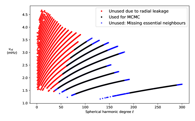
Figure 3: Classification of modes.

4 Results and Discussion

The MCMC analysis is performed for each radial order separately. The current model only considers leakage between modes of the same radial order and hence the ideal way of estimating the parameters would be to estimate all $(a_{3},a_{5})$ at a given radial order by modelling all the cross-spectra at the same radial order. However, this makes the problem computationally very demanding as the MCMC method used requires at least $2k+1$ random walkers for $k$ different parameters to be fit. To work around this, we break the entire set of parameters into chunks of 40 pairs, while ensuring an overlap of 10 pairs between the chunks. In Table 1, we list the set of $\ell$’s for which MCMC sampling is performed and parameters are estimated.

Figure 1 marks the multiplets $(n,\ell)$ available from the HMI pipeline. The multiplets whose modes are used for this study are labelled as black dots. The red dots, which are located at lower $\ell$, correspond to those modes which have contributions from neighbouring radial orders within the temporal-frequency window. This gets worse for $\ell<20$, where contributions from neighbouring radial orders may be seen even near central peaks. Modelling these spectra would require including coupling across radial orders, which is not the case in the present analysis. Thus we only use modes corresponding to $\nu_{n\ell}/\ell<45$. Figure 1 also marks unused HMI-resolved modes as blue dots on either side of the black dots (used modes). This is because we consider only modes that may be fully modelled with parameters available from the HMI pipeline. Modelling a the degree $\ell$ requires mode parameters corresponding to modes from $(\ell-\delta\ell)$ to $(\ell+\delta\ell)$. The existence of unresolved modes (with no mode-parameter information from the HMI pipeline) in this region means that modelling is incomplete, i.e., there would be peaks in the observed spectrum that are missed by the model. Hence, such modes are not considered for the present work. For any given radial order, the first $\delta\ell$ and the last $\delta\ell$ modes cannot be modelled and thus we see blue points on either side of the set of black dots in Figure 1.

The results of the MCMC analysis at all the radial orders are combined and presented in Figure 6. We note that that the confidence intervals become larger for higher $\nu/\ell$. The reasons for this are discussed in Section 4.2. Estimates of $a$-coefficients are largely in agreement with the splitting coefficients — although the most probable values of the coupling-derived parameters are different from their splitting counterparts, they predominantly lie within the 1-$\sigma$ confidence interval. The confidence intervals of $a_{3}$ and $a_{5}$ are nearly the same size. We obtain better results, in terms of the spread in the inferred $a_{3}$-coefficients, than W13. This may be attributed to the consideration of data variance as well as simultaneous fitting for model parameters using a Bayesian approach. For instance, the spread of $a_{3}$ in the range $0<\nu/\ell\lesssim 40$ is seen to be in the range 7.5–30 nHz in W13, whereas our estimates are in the range 15–26 nHz. The present method allows us to quantify the 1-$\sigma$ confidence interval around the most probable values for estimated $a$-coefficients, whereas W13 have shown only inversion values of $a$-coefficients without their respective uncertainties. However, we also note that the estimates of $a_{5}$ from Bayesian analysis are comparable to the least-squares inversions of W13.

4.1 Reconstructed power and cross spectra

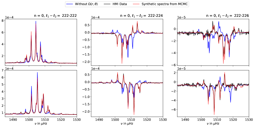
Figure 4: Cross spectrum for $\ell=222$ and $\Delta\ell=0,2,4$. The upper panels correspond to $m^{+}$ and lower panels to $m^{-}$. The black curve shows observed data. The blue curve is the model before considering eigenfunction coupling and the red curve corresponds to model constructed using parameters estimated from MCMC.

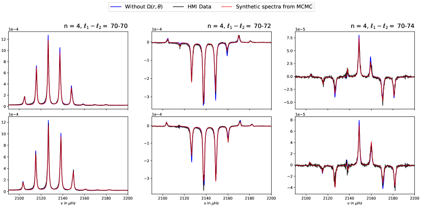
Figure 5: Cross spectrum for $\ell=70$ and $\Delta\ell=0,2,4$. The upper panels correspond to $m^{+}$ and lower panels to $m^{-}$. The black curve shows observed data. The blue curve is the model before considering eigenfunction coupling and the red curve corresponds to the model constructed using parameters estimated from MCMC.

The $a$-coefficients obtained from the MCMC analysis are used to reconstruct cross-spectra, e.g., Figure 4 shows the cross spectrum for $(n=0,\ell=222)$. It may be seen that, before considering eigenfunction corrections (in the absence of differential rotation), the spectrum shown in blue is considerably different — in both magnitude and sign — from the observed data. After including eigenfunction corrections, which have been estimated from MCMC, we see that the model is in close agreement with the data. In the intermediate-$\ell$ range, we show cross-spectra for $(n=4,\ell=70)$ in Figure 5. The corrections due to eigenfunction distortion are markedly less significant when compared to $(\ell=222,n=0)$, demonstrating loss of sensitivity of the model to the coupling coefficients.

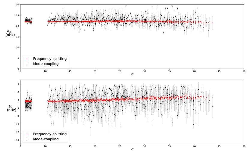
Figure 6: Inferred $a_{3}$ and $a_{5}$ coefficients from MCMC are shown as black dots with 1-$\sigma$ confidence intervals. The values from frequency splitting are shown in red.

4.2 Sensitivity of $a$-coefficients to differential rotation

Mode coupling has diminished sensitivity in estimating $a$-coefficients for low-$\ell$ modes. The coupling coefficients $c_{\ell}^{\ell+p}$ depend on the real and imaginary parts of $b_{k}$. Differential rotation contributes to only the real part of $b_{k}$ (Eqn. [16]) and the dependence on $\ell$ appears through the factor $\ell(\partial\omega_{nl}/\partial\ell)^{-1}$. The plot of eigenfrequencies $\omega_{n\ell}$ against $\ell$ is known to flatten for higher $\ell$. Hence, $\partial\omega_{n\ell}/\partial\ell$ is large for small $\ell$ and small for large $\ell$ (see Figure 1 in Rhodes et al., 1997). This results in $b_{k}$ being small for low $\ell$ and its magnitude increases with $\ell$, causing this decreased sensitivity to low $\ell$. The lower sensitivity implies that the misfit function $S$ is flatter at lower $\ell$. To demonstrate this, we compute $S$ over $\ell=80$–245 for a range of values of $a-$coefficients and determine how wide or flat $S$ is in the neighbourhood of the optimal solution.

Figure 7 shows that the misfit is wide for $\ell=80$ and it becomes sharper with increasing $\ell$. As the highest-resolved mode for $n=1$ corresponds to $\ell=179$, we consider the radial order $n=0$ in order to study this in an extended region of $\ell$. The first two panels show the colour map of the misfit function. Near the optimal value $a^{n\ell}_{s}/a^{n\ell}_{FS}=1$, the synthetic misfit falls to $0$. This is possible as the synthetic data is noise free and it can be completely modeled. The misfit increases on either side of the optimum value. The second panel shows the scaled misfit for HMI data, which is close to $1$ at the optimum, increasing on either side of the optimal value. We see the dark patch become wider at lower $\ell$, indicating the flatness of the misfit function for low $\ell$. The likelihood function, which is defined to be $\exp(-S)$, is approximated as a Gaussian in the vicinity of the optimum. The width of this Gaussian is treated as a measure of the width of the misfit function $S$, with wider misfit implying lower sensitivity to $a-$coefficients. This is shown in the third panel of Figure 7, where we see a decreasing trend in misfit width, indicating that the sensitivity of mode coupling increases with $\ell$.

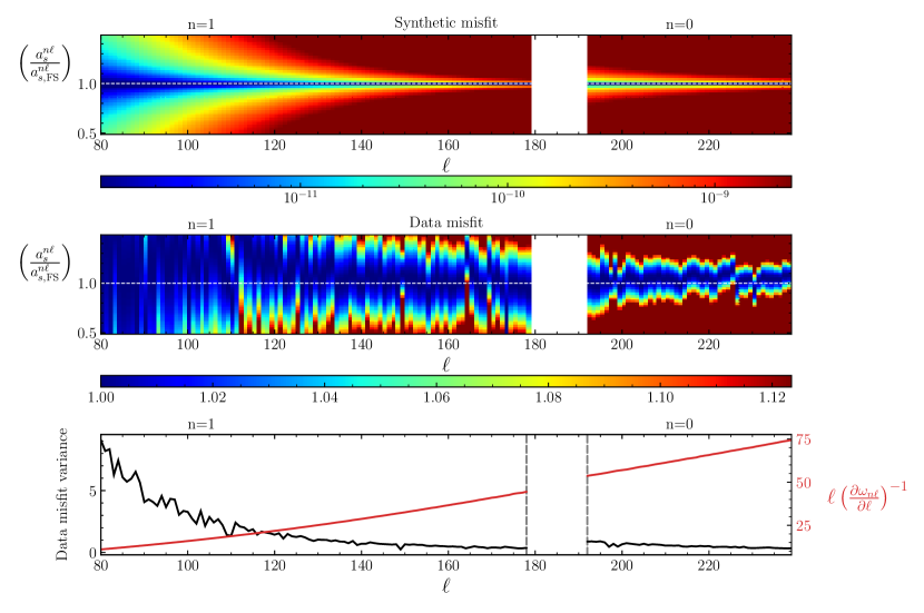
Figure 7: Sensitivity of spectral fitting to $a$-coefficients as a function of angular degree $\ell$. Top panel shows the variation of misfit between synthetic data calculated using frequency-splitting $a$-coefficients $a_{s,\mathrm{FS}}^{n\ell}$ and synthetic spectra computed from a scaled set of $a$ coefficients $a_{s}^{n\ell}$. A well-defined minimum along $a_{s}^{n\ell}/a_{s,\mathrm{FS}}^{n\ell}=1.0$, which broadens towards smaller $\ell$, shows a drop in sensitivity of the spectra to variations in $a$ coefficients, as predicted by theory. Middle panel shows the sensitivity of $a$ coefficients, but now computed using the misfit between HMI and synthetic spectra computed from a scaled set of $a$ coefficients $a_{s}^{n\ell}$. While it has the same qualitative drop in $a$-coefficient sensitivity for decreasing $\ell$, the ridge of the minimum (darkest patch) is seen to deviate from $a_{s,\mathrm{FS}}^{n\ell}$. Bottom panel shows in black the effective variance of misfit for each $\ell$. The narrowing confinement of the data misfit towards higher $\ell$ is seen as a decreasing effective variance with increasing $\ell$. The red line shows the increase in the factor $\ell/(\partial\omega_{n\ell}/\partial\ell)$ that enhances sensitivity at higher $\ell$, as predicted by Eqn. (18). The areas corresponding to radial orders $n=0,1$ are indicated on top of each plot.

4.3 Scaling factor for synthetic spectra

The model constructed using mode parameters obtained from the HMI pipeline needs to be scaled to match the observations. This scaling factor has to be empirically determined. Since there is no well-accepted convention to estimate this factor, it is worthwhile to explore different methods of its estimating. We employ three different methods to infer the scale factor and show that the results are nearly identical.

• Consider all the power spectra for a given radial order and perform a least-squares fitting for the scale factor $N_{0}$.

• Fit for the scale factor $N_{\ell}$ as a function of the spherical harmonic degree $\ell$ by considering all power spectra at a given radial order.

• Include the scale factor as an independent parameter to be estimated in the MCMC analysis.

Figure 8 shows that all the independent ways of estimating the scale factor are within 5% of each other, indicating robustness.

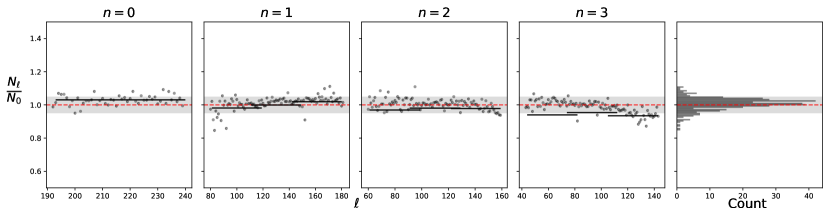
Figure 8: The red line corresponds to $N_{0}$. The gray region corresponds to 5% error from $N_{0}$. The gray points correspond to $N_{\ell}$ and the solid black lines are from each MCMC simulation. The right-most panel shows the histogram of all the gray points, taken from all radial orders.

4.4 How good is the isolated multiplet approximation for $\ell\leq 300$?

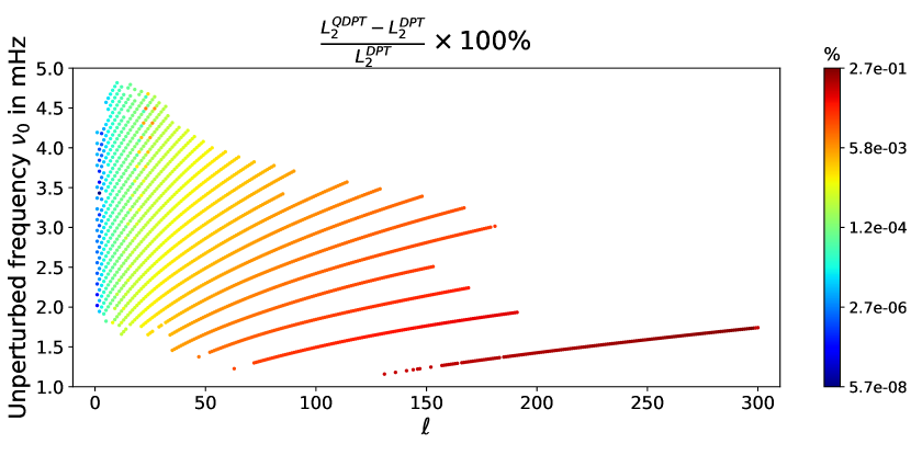
Figure 9: The relative offset of $L_{2}^{\text{QDPT}}$ as compared to that of $L_{2}^{\text{DPT}}$ (see Eqn [30,31]) under the perturbation of an axisymmetric differential rotation $\Omega(r,\theta)$ as observed in the Sun. An increase in intensity of the color scale indicates worsening of the isolated multiplet approximation. The measures of offset are plotted for the HMI-resolved multiplets shown in Figure 1.

Estimation of $a$ coefficients through frequency splitting measurements assumes validity of the isolated multiplet approximation using degenerate perturbation theory (DPT). However, an inspection of the distribution of the multiplets in $\nu-\ell$ space (as shown in Fig. [1]) shows that it is natural to expect this approximation to worsen with increasing $\ell$. This necessitates carrying out frequency estimation respecting cross-coupling of modes across multiplets, also known as quasi-degenerate perturbation theory (QDPT). A detailed discussion on DPT and QDPT in the context of differential rotation can be found in Ritzwoller & Lavely (1991) and Lavely & Ritzwoller (1992). In this section we discuss the goodness of the isolated multiplet approximation in estimating $a_{n\ell}$ due to $\Omega(r,\theta)$ for all the HMI-resolved modes shown in Figure 1. A similar result but for $\ell\leq 30$ was presented in Appendix G of Das et al. (2020). In Figure 9 we color code multiplets to indicate the departure of frequency shifts obtained from QDPT $\delta{}_{n}\omega{}_{\ell m}^{Q}$ as compared to shifts obtained from DPT $\delta{}_{n}\omega{}_{\ell m}^{D}$. Strictly speaking, carrying out the eigenvalue problem in the QDPT formalism causes garbling of the quantum numbers —$n$, $\ell$, and $m$ are no longer good quantum numbers— and prevents a one-to-one mapping of unperturbed to perturbed modes. This prohibits an explicit comparison of frequency shifts on a singlet-by-singlet basis. However, modes belonging to the same multiplet can still be identified visually and grouped together. So, to quantify the departure of $\delta{}_{n}\omega{}_{\ell m}^{Q}$ from $\delta{}_{n}\omega{}_{\ell m}^{D}$ we calculate the Frobenius norm of these frequency shifts corresponding to each multiplet:

$$L_{2}^{\text{QDPT}} = \sqrt{\sum_{m}(\delta{}_{n}\omega{}_{\ell m}^{\text{Q}})^{2}}\qquad\text{for cross-coupling,}$$ (30)

$$L_{2}^{\text{DPT}} = \sqrt{\sum_{m}(\delta{}_{n}\omega{}_{\ell m}^{\text{D}})^{2}}\qquad\text{for self-coupling.}$$ (31)

The color scale intensity in Figure 9 indicates the relative offset of $L_{2}^{\text{QDPT}}$ as compared to $L_{2}^{\text{DPT}}$ for a multiplet $(n,\ell)$ marked as an ‘o’. Larger offset indicates the degree of worsening of the isolated multiplet approximation. We find that the largest error incurred using DPT instead of QPDT is 0.27% this is found to be at $\ell=300$. This clearly shows that even for the $f$ mode (which is the most susceptible to errors) the frequency splitting $a$-coefficients are exceptionally accurate.

5 Conclusion

Most of what is currently known about solar differential rotation is derived from from $a$-coefficients using frequency splitting measurements. Inferring these $a$-coefficients involves invoking the isolated multiplet approximation based on degenerate perturbation theory. Although this approximation works well even for high $\ell\leq 300$ modes, reasons motivating the need to investigate the possibility of erroneous $a$-coefficients from frequency splitting measurements at even higher $\ell$ stem from a combination of two effects, namely, the increasing proximity of modes (in frequency) along the same radial branch, and spectral-leakage from neighbouring modes. Partial visibility of the Sun causes broadening of peaks in the spectral domain, referred to as mode leakage (Schou & Brown, 1994; Hanasoge, 2018). This causes proximal modes at high $\ell$ to widen and resemble continuous ridges in observed spectra. As a result, spectral-peak identification for frequency-splitting measurements are harder and increasingly inaccurate. Moreover, since the $a$-coefficient formalism breaks down for non-axisymmetric perturbations, considering techniques which respect cross-coupling becomes indispensable. Thus, mode coupling becomes more relevant in these regimes, and it is important to investigate the potential of mode-coupling techniques as compared to frequency splittings. Hence, this study was directed towards answering the following broad questions. (i) Can mode-coupling via MCMC use information stored in eigenfunction distortions to constrain differential rotation as accurately as frequency splittings? This would also serve to compare the potential of a Bayesian approach with the least square inversion performed in W13. (ii) Can this technique further increase the accuracy of $a_{n\ell}$ at $\ell\geq 150$? We already know that higher $\ell$ estimates are increasingly precise and accurate from W13. (iii) What are the uncertainties in estimating $a_{n\ell}$ using mode-coupling theory and do they fall within 1-$\sigma$ of frequency splitting estimates? (iv) Why are mode-coupling results poorer in the low $\ell$ regime? This is seen in earlier studies, which aimed to go deeper into the convection zone and obtained significantly imprecise and inaccurate results (Woodard et al., 2013; Schad & Roth, 2020).

The approach in this study is broadly based on the theoretical formulations from V11 and modelling from W13. However, the novelty of the current work lies in 3 main aspects. (a) The MCMC analysis enabled exploration of the complete parameter space, and it was found that the chosen misfit function is unimodal in nature, for all degrees $\ell$ and radial orders $n$. This establishes that the method of normal-mode coupling does return a unique value of $(a_{3},a_{5})$. (b) Leakage of power occurs for modes in the same radial order $n$ and hence the determination of $(a_{3},a_{5})$ in a consistent manner would involve simultaneous estimation of splitting coefficients for all $\ell$ and the same radial order. However, the number of parameters is large and hence we break it into chunks of 40 pairs of $(a_{3},a_{5})$ per MCMC, with an overlap of $N_{o}$ pairs of the parameters between two different chunks. To settle on a reasonable value of $N_{o}$, we perform a simple experiment. From MCMC simulations with different overlap numbers $N_{o}=\{0,2,4,6,8,10\}$, we find that for $N_{o}>6$, the inferred $a$-coefficients vary less than 1-$\sigma$ and therefore reasonably stable for larger $N_{o}$. Hence, we choose the modal overlap number $N_{o}=10$ for computation at all radial orders. (c) Since a large number of splitting coefficients are determined simultaneously, a corresponding number of spectra is used. Hence, estimation of the data variance becomes critical in order to appropriately weight different data points according to their noise levels. These improvements lead to a better estimate of differential rotation using mode coupling.

The inference of rotation at lower $\ell$ ($<50$) suffers for two reasons. (a) Low sensitivity of the model to the $a$-coefficients. (b) Proximity of modes of radial orders $(n+1)$ and $(n-1)$ to modes at radial order $n$. Since the current model only accounts for leakage of power within the same radial order, a chosen frequency window in data would contain peaks from neighboring radial orders, which are not modelled. Hence, an improvement might be achieved at lower $\ell$ by modelling the interaction of modes of different radial orders.

Finally, in this study we also show that even though frequency splitting is much more precise for low $\ell\leq 150$, mode coupling estimates of differential rotation improves at high $\ell\geq 200$. Therefore, it is expected that mode-coupling would be comparable to (or possibly more accurate than) frequency splitting for very high $\ell\geq 300$. This would then allow one to compare mode-coupling estimates of shallow, small-scale structures with results from methods in local helioseismology. Going this high in angular degree for mode-coupling, however, introduces some challenges: (a) The computation of leakage matrices for high $\ell$ is very expensive. (b) $\partial\omega/\partial\ell$ decreases as $\ell$ grows and the spectrum becomes a continuous ridge in frequency space making it harder to resolve the modes completely.

In conclusion, there remains scope for improvement and related lines of study. In this study, we have ignored the even-$s$ components of $\Omega_{s}$, which are the NS-asymmetric components of differential rotation. These components have been estimated to be small at the surface and are anticipated to be small in the interior. However, this assumption may be premature given that prior estimates of interior rotation-asymmetries are based on non-seismic surface measurements. Since the V11 formalism is capable of accommodating the estimation of even-$s$ components as well, this could be the focus of a future investigation. Additionally, the current analysis was performed after summing up the stacked cross-spectrum. Although this was done to improve the signal-to-noise ratio, the spectrum at different azimuthal orders $m$ are not identical. Hence a more complete computation would involve the misfit computed using the full spectrum as a function of $m$. This may possibly lead to better results of the $a$-coefficients, as there exists structure in the azimuthal order (see Fig. [2]), which is lost after summation.

The authors of this study are grateful to Jesper Schou (Max Planck Institute for Solar System Research) for numerous insightful discussions as well as detailed comments that helped us improve the quality of the manuscript. The authors thank the anonymous referee for valuable suggestions that helped improve the text and figures in this manuscript.

Appendix A Spherical harmonics symmetry relations

Consider a time-varying, real-valued scalar field on a sphere $\phi(\theta,\phi,t)$. The spherical harmonic components are given by

$$\phi^{l,|m|}(t)=\int_{\Omega}{\mathrm{d}}\Omega Y^{*l,|m|}(\theta,\phi)\phi(\theta,\phi,t)=(-1)^{|m|}\int_{\Omega}{\mathrm{d}}\Omega Y^{l,-|m|}\phi(\theta,\phi,t)=(-1)^{|m|}\phi^{*l,-|m|}(t)$$ (32)

where $d\Omega$ is the area element, the integration being performed over the entire surface of the sphere. After performing a temporal Fourier transform, we have

$$\phi^{l,|m|}(\omega)=\frac{1}{\sqrt{2\pi}}\int_{-\infty}^{\infty}{\mathrm{d}}te^{-i\omega t}\phi^{l,|m|}(t)=(-1)^{|m|}\frac{1}{\sqrt{2\pi}}\int_{-\infty}^{\infty}{\mathrm{d}}te^{-i\omega t}\phi^{*l,-|m|}(t)$$ (33)

$$\phi^{*l,-|m|}(\omega)=\frac{1}{\sqrt{2\pi}}\int_{-\infty}^{\infty}{\mathrm{d}}te^{i\omega t}\phi^{*l,-|m|}(t)=(-1)^{|m|}\phi^{l,|m|}(-\omega)\implies\phi^{l,-|m|}(\omega)=(-1)^{|m|}\phi^{*l,|m|}(-\omega)$$ (34)

Appendix B MCMC: An illustrative Case

We present an MCMC estimation of $a$-coefficients using a smaller set of modes (and hence model parameters). The smaller number of model parameters lets us present all the marginal probabilities in a single plot. The MCMC walkers are shown in Figure 10. In spite of using a flat prior, the likelihood function is sharp enough to bias the walkers to move towards the region of optimal solution within $\sim 500$ iterations. It can be seen that different walkers start off randomly at different locations in parameter space and ultimately converge to the same region around the optimal solution. After removing the iterations from the “burn-in” period, where the walkers are still exploring a larger parameter space, histograms are plotted and marginal probability distributions are obtained. Figure 11 shows one such estimation of $(a_{3},a_{5})$ for $n=0$ and $\ell$ in the range $200$ to $202$. It can be seen that the marginal posterior probability distributions for each of the parameters are unimodal. This tells us that the currently defined misfit function has a unique minimum. Note that this distribution was obtained using a flat prior and hence the resulting posterior distributions are essentially sampling the likelihood function. It is also worth noting that for the range of $\ell$’s chosen, the confidence intervals are $<1$ nHz.

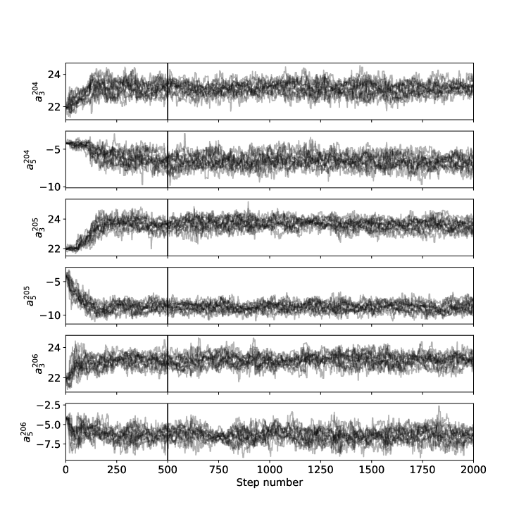
Figure 10: Each parameter is shown in a different figure to indicate the value as a function of the Markov Chain step number. The first few “burn-in” values are discarded and only the values beyond the vertical line are considered to obtain the probability distributions.

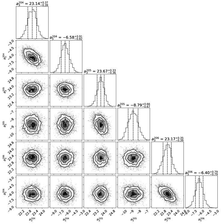
Figure 11: Cross-correlation of model parameters and the marginal probability of the model parameters.

References

- Antia et al. (2013) Antia, H. M., Chitre, S. M., & Gough, D. O. 2013, MNRAS, 428, 470, doi: 10.1093/mnras/sts040
- Basu & Antia (2003) Basu, S., & Antia, H. M. 2003, The Astrophysical Journal, 585, 553, doi: 10.1086/346020
- Basu et al. (1999) Basu, S., Antia, H. M., & Tripathy, S. C. 1999, ApJ, 512, 458, doi: 10.1086/306765
- Brown et al. (1989) Brown, T. M., Christensen-Dalsgaard, J., Dziembowski, W. A., et al. 1989, ApJ, 343, 526, doi: 10.1086/167727
- Brown & Morrow (1987) Brown, T. M., & Morrow, C. A. 1987, ApJ, 314, L21, doi: 10.1086/184843
- Chandrasekhar & Kendall (1957) Chandrasekhar, S., & Kendall, P. C. 1957, The Astrophysical Journal, 126, 457
- Chaplin et al. (2004) Chaplin, W. J., Sekii, T., Elsworth, Y., & Gough, D. O. 2004, MNRAS, 355, 535, doi: 10.1111/j.1365-2966.2004.08338.x
- Chaplin et al. (1999) Chaplin, W. J., Christensen-Dalsgaard, J., Elsworth, Y., et al. 1999, MNRAS, 308, 405, doi: 10.1046/j.1365-8711.1999.02691.x
- Charbonneau (2005) Charbonneau, P. 2005, Living Reviews in Solar Physics, 2, 2
- Chatterjee & Antia (2009) Chatterjee, P., & Antia, H. M. 2009, ApJ, 707, 208, doi: 10.1088/0004-637X/707/1/208
- Christensen–Dalsgaard (2003) Christensen–Dalsgaard, J. 2003, Lecture Notes on Stellar Oscillations, 5th edn.
- Christensen & Meyer (1998) Christensen, N., & Meyer, R. 1998, Phys. Rev. D, 58, 082001, doi: 10.1103/PhysRevD.58.082001
- Christensen-Dalsgaard et al. (1996) Christensen-Dalsgaard, J., Dappen, W., Ajukov, S. V., et al. 1996, Science, 272, 1286
- Claverie et al. (1981) Claverie, A., Isaak, G. R., McLeod, C. P., van der Raay, H. B., & Roca Cortes, T. 1981, Nature, 293, 443, doi: 10.1038/293443a0
- Couvidat et al. (2003) Couvidat, S., García, R. A., Turck-Chièze, S., et al. 2003, ApJ, 597, L77, doi: 10.1086/379698
- Cutler (2017) Cutler, C. 2017, Using eigenmode-mixing to measure or constrain the Sun’s interior B-field. https://arxiv.org/abs/1706.07404
- Dahlen & Tromp (1998) Dahlen, F. A., & Tromp, J. 1998, Theoretical Global Seismology (Princeton University Press)
- Das et al. (2020) Das, S. B., Chakraborty, T., Hanasoge, S. M., & Tromp, J. 2020, ApJ, 897, 38, doi: 10.3847/1538-4357/ab8e3a
- Duvall et al. (1996) Duvall, Jr., T. L., D’Silva, S., Jefferies, S. M., Harvey, J. W., & Schou, J. 1996, Nature, 379, 235, doi: 10.1038/379235a0
- Duvall & Harvey (1984) Duvall, Jr., T. L., & Harvey, J. W. 1984, Nature, 310, 19
- Dziembowski & Goode (2004) Dziembowski, W. A., & Goode, P. R. 2004, ApJ, 600, 464, doi: 10.1086/379708
- Eff-Darwich et al. (2002) Eff-Darwich, A., Korzennik, S. G., & Jiménez-Reyes, S. J. 2002, ApJ, 573, 857, doi: 10.1086/340747
- Fan (2009) Fan, Y. 2009, Living Reviews in Solar Physics, 6, 4, doi: 10.12942/lrsp-2009-4
- Foreman-Mackey et al. (2013) Foreman-Mackey, D., Hogg, D. W., Lang, D., & Goodman, J. 2013, PASP, 125, 306, doi: 10.1086/670067
- Freidberg (2014) Freidberg, J. P. 2014, Ideal MHD (Cambridge University Press), doi: 10.1017/CBO9780511795046
- Giles et al. (1997) Giles, P. M., Duvall, Jr., T. L., Scherrer, P. H., & Bogart, R. S. 1997, Nature, 390, 52
- Gilman (1974) Gilman, P. A. 1974, ARA&A, 12, 47, doi: 10.1146/annurev.aa.12.090174.000403
- Gizon et al. (2020) Gizon, L., Cameron, R. H., Pourabdian, M., et al. 2020, Science, 368, 1469, doi: 10.1126/science.aaz7119
- Goodman & Weare (2010) Goodman, J., & Weare, J. 2010, Communications in Applied Mathematics and Computational Science, 5, 65, doi: 10.2140/camcos.2010.5.65
- Gough & Hindman (2010) Gough, D., & Hindman, B. W. 2010, ApJ, 714, 960, doi: 10.1088/0004-637X/714/1/960
- Gough (1990) Gough, D. O. 1990, in Lecture Notes in Physics, Berlin Springer Verlag, Vol. 367, Progress of Seismology of the Sun and Stars, ed. Y. Osaki & H. Shibahashi, 283, doi: 10.1007/3-540-53091-6
- Hanasoge (2018) Hanasoge, S. 2018, ApJ, 861, 46, doi: 10.3847/1538-4357/aac3e3
- Hanasoge et al. (2017) Hanasoge, S. M., Woodard, M., Antia, H. M., Gizon, L., & Sreenivasan, K. R. 2017, MNRAS, 470, 1404, doi: 10.1093/mnras/stx1298
- Howard et al. (1984) Howard, R., Gilman, P. I., & Gilman, P. A. 1984, ApJ, 283, 373, doi: 10.1086/162315
- Howe (2009) Howe, R. 2009, Living Reviews in Solar Physics, 6, 1. https://arxiv.org/abs/0902.2406
- Imada & Fujiyama (2018) Imada, S., & Fujiyama, M. 2018, ApJ, 864, L5, doi: 10.3847/2041-8213/aad904
- Jackiewicz (2020) Jackiewicz, J. 2020, Sol. Phys., 295, 137, doi: 10.1007/s11207-020-01667-3
- Kosovichev et al. (1997) Kosovichev, A. G., Schou, J., Scherrer, P. H., et al. 1997, Sol. Phys., 170, 43
- Larson & Schou (2015) Larson, T. P., & Schou, J. 2015, Sol. Phys., 290, 3221, doi: 10.1007/s11207-015-0792-y
- Lavely & Ritzwoller (1992) Lavely, E. M., & Ritzwoller, M. H. 1992, Philosophical Transactions of the Royal Society of London Series A, 339, 431, doi: 10.1098/rsta.1992.0048
- Libbrecht (1989) Libbrecht, K. G. 1989, ApJ, 336, 1092, doi: 10.1086/167079
- Mdzinarishvili et al. (2020) Mdzinarishvili, T., Shergelashvili, B., Japaridze, D., et al. 2020, Advances in Space Research, 65, 1843 , doi: https://doi.org/10.1016/j.asr.2020.01.015
- Metropolis et al. (1953) Metropolis, N., Rosenbluth, A. W., Rosenbluth, M. N., Teller, A. H., & Teller, E. 1953, J. Chem. Phys., 21, 1087, doi: 10.1063/1.1699114
- Metropolis & Ulam (1949) Metropolis, N., & Ulam, S. 1949, Journal of the American Statistical Association, 44, 335. http://www.jstor.org/stable/2280232
- Miesch (2005) Miesch, M. S. 2005, Living Reviews in Solar Physics, 2, 1
- Rhodes et al. (1997) Rhodes, E. J., J., Kosovichev, A. G., Schou, J., Scherrer, P. H., & Reiter, J. 1997, Sol. Phys., 175, 287, doi: 10.1023/A:1004963425123
- Ritzwoller & Lavely (1991) Ritzwoller, M. H., & Lavely, E. M. 1991, ApJ, 369, 557, doi: 10.1086/169785
- Saha & Williams (1994) Saha, P., & Williams, T. B. 1994, AJ, 107, 1295, doi: 10.1086/116942
- Sambridge & Mosegaard (2002) Sambridge, M., & Mosegaard, K. 2002, Reviews of Geophysics, 40, 1009, doi: 10.1029/2000RG000089
- Schad & Roth (2020) Schad, A., & Roth, M. 2020, ApJ, 890, 32, doi: 10.3847/1538-4357/ab65ec
- Schad et al. (2011) Schad, A., Timmer, J., & Roth, M. 2011, ApJ, 734, 97, doi: 10.1088/0004-637X/734/2/97
- Schad et al. (2013) —. 2013, ApJ, 778, L38, doi: 10.1088/2041-8205/778/2/L38
- Schou & Brown (1994) Schou, J., & Brown, T. M. 1994, A&AS, 107, 541
- Schou et al. (1998) Schou, J., Antia, H. M., Basu, S., et al. 1998, ApJ, 505, 390, doi: 10.1086/306146
- Schou et al. (2012) Schou, J., Scherrer, P. H., Bush, R. I., et al. 2012, Sol. Phys., 275, 229, doi: 10.1007/s11207-011-9842-2
- Sharma (2017) Sharma, S. 2017, ARA&A, 55, 213, doi: 10.1146/annurev-astro-082214-122339
- Thompson et al. (1996) Thompson, M. J., Toomre, J., Anderson, E. R., et al. 1996, Science, 272, 1300, doi: 10.1126/science.272.5266.1300
- Ulrich et al. (1988) Ulrich, R. K., Boyden, J. E., Webster, L., et al. 1988, Sol. Phys., 117, 291, doi: 10.1007/BF00147250
- Vorontsov (2007) Vorontsov, S. V. 2007, MNRAS, 378, 1499, doi: 10.1111/j.1365-2966.2007.11894.x
- Vorontsov (2011) Vorontsov, S. V. 2011, Monthly Notices of the Royal Astronomical Society, 418, 1146, doi: 10.1111/j.1365-2966.2011.19564.x
- Woodard et al. (2013) Woodard, M., Schou, J., Birch, A. C., & Larson, T. P. 2013, Sol. Phys., 287, 129, doi: 10.1007/s11207-012-0075-9
- Woodard (1989) Woodard, M. F. 1989, ApJ, 347, 1176, doi: 10.1086/168206
- Woodard (2000) —. 2000, Sol. Phys., 197, 11, doi: 10.1023/A:1026508211960
- Zhao & Kosovichev (2004) Zhao, J., & Kosovichev, A. G. 2004, ApJ, 603, 776, doi: 10.1086/381489