A practical method for recovering Sturm-Liouville problems from the Weyl function

Abstract

In the paper we propose a direct method for recovering the Sturm-Liouville potential from the Weyl-Titchmarsh $m$-function given on a countable set of points. We show that using the Fourier-Legendre series expansion of the transmutation operator integral kernel the problem reduces to an infinite linear system of equations, which is uniquely solvable if so is the original problem. The solution of this linear system allows one to reconstruct the characteristic determinant and hence to obtain the eigenvalues as its zeros and to compute the corresponding norming constants. As a result, the original inverse problem is transformed to an inverse problem with a given spectral density function, for which the direct method of solution from [28] is applied.

The proposed method leads to an efficient numerical algorithm for solving a variety of inverse problems. In particular, the problems in which two spectra or some parts of three or more spectra are given, the problems in which the eigenvalues depend on a variable boundary parameter (including spectral parameter dependent boundary conditions), problems with a partially known potential and partial inverse problems on quantum graphs.

1 Introduction

We consider the inverse problem of recovering the potential of a Sturm-Liouville equation on a finite interval together with the boundary conditions from values of the Weyl-Titchmarsh $m$-function on a given set of points.

A fundamental result of Marchenko [30] states that the Weyl-Titchmarsh function $m(z)$ determines uniquely the potential $q\in L_{2}(0,\pi)$ as well as the boundary conditions. So some particular inverse problem is solved, at least in theory, if one finds a way to convert it to a corresponding problem for the $m$-function. However, several difficulties arise. For some inverse spectral problems the given spectral data allow one to obtain the values of the $m$-function at any point $z\in\mathbb{C}$. This is the case of the classical inverse problem with a given spectral density function, formula (2.13) below provides the $m$-function. While for many problems only the values of the $m$-function on a countable set of points $\{z_{k}\}_{k=0}^{\infty}$ can be obtained. See Subsection 2.2 and references therein for some examples. Thus one faces two principle questions. Is it possible to recover uniquely the $m$-function from the given values $m(z_{k})$, $k=0,1,\ldots$? If yes, how can that be done?

Since the $m$-function is meromorphic, the unique recovery is always possible if the sequence $\{z_{k}\}_{k=0}^{\infty}$ contains a subsequence $z_{n_{k}}$ converging to a finite limit and such that the values $m(z_{n_{k}})$ are bounded. This is usually not the case when we start with some inverse problem, the points $z_{k}$ are real and go to infinity when $k\rightarrow\infty$. Suppose all the points $z_{k}$ are real. A simple sufficient condition for the unique recoverability of the $m$-function from the given values $m(z_{k})$ was given in [9], and a complete answer was given not so long ago in [20]. Simply speaking, the points $z_{k}$ should be distributed sufficiently densely, like the points obtained as a union of two spectra.

The corresponding results are obtained by using infinite products and analytic continuation. And as it is stated in the following quote [7, p.106],

It is one of the guiding principles of computational analysis that such proofs often lead to elegant mathematics but are useless as far as constructive methods are concerned.

The only constructive method for finding the $m$-function we are aware of is that from [4], [41] (based on the ideas of [34] and [7, Chapter 3]). This algorithm recovers a certain combination of the integral kernel of the transmutation operator with its derivative by using non-harmonic Fourier series. However it works only for sequences $z_{n}$ such that the sequence of functions $\{e^{\pm i\sqrt{z_{n}}t}\}_{n\in\mathbb{N}}$ is a Riesz basis in $L_{2}(-2\pi,2\pi)$, requires additionally a beforehand knowledge of the parameter $\omega$ (depending on the average of the potential $q$ and boundary parameter $H$) and numerical realization of this method is expected to converge slowly (no numerical illustration is provided in [4] or [41]).

We use Fourier-Legendre series to represent the transmutation integral kernel and its derivative. This idea was originally proposed in [26] and resulted in a Neumann series of Bessel functions (NSBF) representation for the solutions and their derivatives of Sturm-Liouville equations. As a result, a constructive algorithm for recovering the $m$-function from its values on a countable set of points is proposed. The problem is reduced to an infinite system of linear equations and the unique solvability of this system is proved. We would like to emphasize that no additional information is necessary beforehand.

Moreover, the proposed method leads to an efficient numerical algorithm. Since the NSBF representation possesses such a remarkable property as a uniform error bound for all real $\lambda>0$, one can obtain any finite set of approximate eigenvalues and corresponding norming constants with a non-deteriorating accuracy. That is, an efficient conversion of the original problem to an inverse problem by a given spectral density function is proposed. The method of solution introduced in [24], [25] and refined in [28] is adapted to recover the potential and the boundary conditions from the spectral density function.

For classical inverse spectral problems there are many results describing to what extent the potential can be recovered from a finite set of spectral data, see, e.g., [17], [32], [37], [35]. For the Weyl function, on the contrary, we are not aware of any single result. It can be seen that the values of $z_{k}$, $0\leq k\leq K$ can be chosen neither from a too small interval nor too sparse. Indeed, taking all the values $z_{k}$ from one spectrum is insufficient to recover the potential. On the other hand, as was mentioned in [7, Subsections 3.10.5 and 3.14], when all the values $z_{k}$ are equal to the first eigenvalue $\lambda_{0}$ (for problems with different boundary conditions), the corresponding numerical problem is extremely ill-conditioned. So the proposed algorithm struggles as well when the points $z_{k}$ either belong to a small interval or are too sparse. Nevertheless, it delivers excellent results for smooth potentials and sufficiently dense points $z_{k}$, does not require any additional information on the potential or boundary conditions and can be applied to a variety of inverse problems for which not so many (if any) specialized algorithms are known. So we believe the presented method will be a starting point for the future research of the question “to which extent a potential can be recovered from a given finite set of values of the Weyl-Titchmarsh $m$-function”, as well as of a new class of numerical methods based on the Weyl-Titchmarsh $m$-function.

The paper is organized as follows. In Section 2 we provide necessary information on the Weyl function, transmutation operators and Neumann series of Bessel functions representations. In Section 3 we show how the inverse problem of recovering the Sturm-Liouville problem from the Weyl function is reduced to an infinite system of linear algebraic equations, prove its unique solvability and show the reduction of the original problem to the classical problem of the recovery of a Sturm-Liouville problem from a given spectral density function; an algorithm is provided. Finally in Section 4 we present several numerical examples illustrating the efficiency and some limitations of the proposed method.

2 Preliminaries

2.1 The Weyl function and spectral data

Let $q\in L_{2}(0,\pi)$ be real valued. Consider the Sturm-Liouville equation

$$-y^{\prime\prime}+q(x)y=\rho^{2}y,\quad x\in(0,\pi),$$ (2.1)

where $\rho\in\mathbb{C}$, with the boundary conditions

$$y^{\prime}(0)-hy(0)=0,\quad y^{\prime}(\pi)+Hy(\pi)=0,$$ (2.2)

where $h$ and $H$ are arbitrary real constants, and the boundary value problem

$$y^{\prime}(0)-hy(0)=1,\quad y^{\prime}(\pi)+Hy(\pi)=0.$$ (2.3)

If $\lambda=\rho^{2}$ is not an eigenvalue of the spectral problem (2.1), (2.2), then the boundary value problem (2.1), (2.3) possesses a unique solution, which we denote by $\Phi(\rho,x)$. Let

$$M(\lambda):=\Phi(\rho,0).$$

The functions $\Phi(\rho,x)$ and $M(\lambda)$ are called the Weyl solution and the Weyl function, respectively. See [42, Section 1.2.4] for additional details.

By $\varphi(\rho,x)$ and $S(\rho,x)$ we denote the solutions of (2.1) satisfying the initial conditions

$$\varphi(\rho,0)=1\quad\text{and}\quad\varphi^{\prime}(\rho,0)=h$$ (2.4)

and

$$S(\rho,0)=0\quad\text{and}\quad S^{\prime}(\rho,0)=1,$$ (2.5)

respectively. Denote additionally for $\lambda=\rho^{2}$

$$\Delta(\lambda):=\varphi^{\prime}(\rho,\pi)+H\varphi(\rho,\pi)\quad\text{and}\quad\Delta^{0}(\lambda):=S^{\prime}(\rho,\pi)+HS(\rho,\pi).$$ (2.6)

Obviously, for all $\rho\in\mathbb{C}$ the function $\varphi(\rho,x)$ fulfills the first boundary condition, $\varphi^{\prime}(\rho,0)-h\varphi(\rho,0)=0$, and thus, the spectrum of problem (2.1), (2.2) is the sequence of numbers $\left\{\lambda_{n}=\rho_{n}^{2}\right\}_{n=0}^{\infty}$ such that

$$\Delta(\lambda_{n})=0.$$

It is easy to see that

$$\Phi(\rho,x)=S(\rho,x)+M(\lambda)\varphi(\rho,x)$$ (2.7)

and

$$M(\lambda)=-\frac{\Delta^{0}(\lambda)}{\Delta(\lambda)}.$$ (2.8)

Moreover, the Weyl function is meromorphic with simple poles at $\lambda=\lambda_{n}$, $n\geq 0$.

Remark 2.1.

There is another common definition of the Weyl-Titchmarsh $m$-function [39], [10], [20]. Let $v(\rho,x)$ be the solution of (2.1) satisfying

$$v(\rho,\pi)=1\quad\text{and}\quad v^{\prime}(\rho,\pi)=-H.$$ (2.9)

Then the Weyl-Titchmarsh $m$-function is defined as

$$m(\rho^{2})=\frac{v^{\prime}(\rho,0)}{v(\rho,0)}.$$ (2.10)

One can verify that

$$m(\rho^{2})=h-\frac{\Delta(\rho^{2})}{\Delta^{0}(\rho^{2})}=h+\frac{1}{M(\rho^{2})},$$ (2.11)

that is, the functions $m$ and $M$ can be easily transformed one into another.

Denote additionally

$$\alpha_{n}:=\int_{0}^{\pi}\varphi^{2}(\rho_{n},x)\,dx.$$ (2.12)

The set $\left\{\alpha_{n}\right\}_{n=0}^{\infty}$ is referred to as the sequence of norming constants of problem (2.1), (2.2).

Theorem 2.2 (see [42, Theorem 1.2.6]).

The following representation holds

$$M(\lambda)=\sum_{n=0}^{\infty}\frac{1}{\alpha_{n}(\lambda-\lambda_{n})}.$$ (2.13)

Let us formulate the inverse Sturm-Liouville problem.

Problem 2.3 (Recovery of a Sturm-Liouville problem from its Weyl function).

Given the Weyl function $M(\lambda)$, find a real valued $q\in L_{2}(0,\pi)$, and the constants $h$, $H\in\mathbb{R}$, such that $M(\lambda)$ be the Weyl function of problem (2.1), (2.2).

We refer the reader to [42, Theorem 1.2.7] for the result on the unique solvability of Problem 2.3.

Having the Weyl function known completely, one can recover the sequence $\{\lambda_{n}\}_{n=0}^{\infty}$ as the sequence of its poles, and the sequence $\{\alpha_{n}\}_{n=0}^{\infty}$ can be immediately obtained from the corresponding residuals, the formula (1.2.14) from [42] states that

$$\alpha_{n}=\frac{1}{\operatorname{Res}_{\lambda=\lambda_{n}}M(\lambda)}=-\frac{1}{\Delta^{0}(\lambda_{n})}\cdot\left.\frac{d}{d\lambda}\Delta(\lambda)\right|_{\lambda=\lambda_{n}}.$$ (2.14)

Hence reducing the inverse problem to recovering the Sturm-Liouville problem by its spectral density function. Or, by taking the sequences of poles and zeros of the Weyl function one can reduce Problem 2.3 to recovering the Sturm-Liouville problem by two spectra, see [42, Remark 1.2.3].

However the situation is more complicated if one looks for a practical method of recovering $q$, $h$ and $H$ from the Weyl function given only on a countable (even worse, finite) set of points from some (small) interval. The direct reduction to the inverse problems considered, in particular, in [28], is not possible. Let us formulate the corresponding problem and state some sufficient results for its unique solvability.

Problem 2.4 (Recovery of a Sturm-Liouville problem from its Weyl function given on a countable set of points).

Given the values $M_{n}=M(z_{n})$, $M_{n}\in\mathbb{C}\cup\{\infty\}$, of the Weyl function $M(\lambda)$ on a set of points $\{z_{n}\}_{n=0}^{\infty}$, find a real valued $q\in L_{2}(0,\pi)$, and the constants $h$, $H\in\mathbb{R}$, such that the Weyl function of problem (2.1), (2.2) takes the values $M_{n}$ at the points $z_{n}$, $n\geq 0$.

It is easy to see that Problem 2.4 is not always uniquely solvable. The following result shows that choosing the set of points $z_{n}$ “sufficiently dense” can guarantee the unique solvability.

Theorem 2.5 ([9, Theorem 2.1]).

Let $a_{+}=\max(a,0)$ for $a\in\mathbb{R}$. Let $\{z_{n}\}_{n=0}^{\infty}$ be a sequence of distinct positive real numbers satisfying

$$\sum_{n=1}^{\infty}\frac{\left(z_{n}-\frac{1}{4}n^{2}\right)_{+}}{n^{2}}<\infty.$$ (2.15)

Let $m_{1}$ and $m_{2}$ be Weyl-Titchmarsh $m$-functions for two Sturm-Liouville problems having the potentials $q_{1}$ and $q_{2}$ and the constants $H_{1}$ and $H_{2}$, correspondingly. Suppose that $m_{1}(z_{n})=m_{2}(z_{n})$ for all $n\in\mathbb{N}_{0}$. Then $m_{1}=m_{2}$ (and hence $q_{1}=q_{2}$ a.e. on $[0,\pi]$ and $H_{1}=H_{2}$).

See also [20, Theorem 1.5] for the necessary and sufficient result.

2.2 Some inverse problems which can be reduced to Problem 2.4

Below we briefly present some inverse problems, omitting any additional details like the conditions on a spectra ensuring the uniqueness of the solution. They can be consulted in the provided references.

2.2.1 Two spectra

Consider the second set of boundary conditions

$$y(0)=0,\quad y^{\prime}(\pi)+Hy(\pi)=0.$$ (2.16)

Let us denote the spectrum of problem (2.1), (2.16) as $\left\{\nu_{n}=\mu_{n}^{2}\right\}_{n=0}^{\infty}$.

The inverse problem consists in recovering $q$, $h$ and $H$ from given two spectra, $\{\lambda_{n}\}_{n=0}^{\infty}$ and $\{\nu_{n}\}_{n=0}^{\infty}$. Note that this problem coincides with the one considered in [28] if one changes $x$ by $\pi-x$ and $h\leftrightarrow H$. Now the equalities

$$M(\lambda_{n})=\infty\quad\text{and}\quad M(\nu_{n})=0,$$

can be easily checked and give the reduction of the two spectra inverse problem to Problem 2.4.

2.2.2 Eigenvalues depending on a variable boundary parameter

There is a class of inverse problems where it is asked to recover the potential from given parts of three spectra [9], four spectra [33], $N$ spectra [19]. All these problems can be regarded as special cases of the following inverse problem. Suppose the sequences of numbers $\{\tilde{\lambda}_{n}\}_{n=0}^{\infty}$ and $\{h_{n}\}_{n=0}^{\infty}$ are given and such that $\tilde{\lambda}_{n}$ is an eigenvalue (does not refer to $n$-th indexed eigenvalue) of the problem (2.1) with the boundary conditions

$$y^{\prime}(0)-h_{n}y(0)=0,\quad y^{\prime}(\pi)+Hy(\pi)=0.$$ (2.17)

The problem is to recover the potential $q$. We refer the reader to [7, §3.10.5 and §3.15] for some discussion and numerical results.

The reduction to Problem 2.4 follows immediately when one observes that (2.17) leads to

$$m(\tilde{\lambda}_{n})=h_{n}.$$

2.2.3 Partially known potential

The Hochstadt-Lieberman inverse problem from [18] reads as follows: suppose we are given the spectrum of the problem (2.1), (2.2) and the potential $q$ is known on the segment $[0,\pi/2]$. Recover $q$ on the whole segment $[0,\pi]$. See also [11], [9] for the case when the potential is known on a different portion of the segment. If the potential is known on less than half of the segment, more than one spectrum is necessary to recover the potential uniquely. For that reason the general formulation of the problem is as follows. Suppose $a\in(0,\pi)$ and the potential $q$ is known on $[0,a]$. Moreover, two sequences of numbers are given as in Subsubsection 2.2.2. Recover $q$ on the whole $[0,\pi]$.

Let $m(x,\rho^{2})$ define the $m$-function on $[x,\pi]$ with the same boundary condition (2.9), i.e.,

$$m(x,\rho^{2})=\frac{v^{\prime}(\rho,x)}{v(\rho,x)}.$$

Consider an eigenvalue $\tilde{\lambda}_{n}=\rho_{n}^{2}$ and the corresponding boundary constant $h_{n}$. Then

$$m(0,\tilde{\lambda}_{n})=m(\tilde{\lambda}_{n})=h_{n},$$

hence we may consider the following Cauchy problem for equation (2.1)

$$v(\rho_{n},0)=1,\quad v^{\prime}(\rho_{n},0)=h_{n}.$$

Solving it on $[0,a]$ (in practice it can be done efficiently for a large set of $\tilde{\lambda}_{n}$ using the method developed in [26]), we obtain values $v(\rho_{n},a)$ and $v^{\prime}(\rho_{n},a)$, hence, $m(a,\tilde{\lambda}_{n})$. And by rescaling we reduce the problem of a partially known potential to Problem 2.4.

2.2.4 Problems with analytic functions in the boundary condition

The following spectral parameter dependent boundary condition was considered in [4], [5], [41]

$$f_{1}(\lambda)y^{\prime}(0)+f_{2}(\lambda)y(0)=0,$$ (2.18)

where $f_{1}$ and $f_{2}$ are entire functions, not vanishing simultaneously. The second boundary condition is the same as in (2.2). The functions $f_{1}$ and $f_{2}$ are supposed to be known, and an inverse problem consists in recovering the potential $q$ and the constant $H$ by the given parameter $\omega_{2}$ (see (2.39)), spectra $\lambda_{n}$ and corresponding multiplicities $m_{n}$. See also [38] for a general spectral theory of such problems.

Supposing for simplicity that all the eigenvalues are simple, i.e., $m_{n}=1$ for all $n$, the problem immediately reduces to Problem 2.4, since

$$m(\lambda_{n})=-\frac{f_{2}(\lambda_{n})}{f_{1}(\lambda_{n})}.$$

Many inverse problems can be reduced to a problem having boundary condition (2.18). In particular, the Hochstadt-Lieberman problem, the inverse transmission eigenvalue problem, partial inverse problems for quantum graphs. See [41] and references therein for more details.

2.3 Some practical applications

Inverse Sturm-Liouville problems arise in numerous applied field. For some examples in vibration models we refer to the book [14], for some biomedical engineering applications to the review [15], while here we add two more examples from different areas of physics.

In studying quantum physical properties of quantum dot nanostructures the problem of recovering symmetric potentials from a finite number of experimentally obtained eigenvalues is of considerable importance (see, e.g., [23]). Mathematically this means that the potential $q$ in (2.1) is symmetric: $q(x)=q(\pi-x)$, and a finite part of one spectrum is given. For simplicity let us suppose that it corresponds to the Dirichlet conditions. Then, as it is well known (see [7, p. 103]), this problem reduces to the two spectra problem on the interval $(0,\pi/2)$. Indeed, for the eigenfunctions we have $y_{n}(x)=y_{n}(\pi-x)$ if $n$ is odd and $y_{n}(x)=-y_{n}(\pi-x)$ if $n$ is even. Thus, $y_{n}(0)=0$, $y_{n}(\pi/2)=0$ if $n$ is even and $y_{n}(0)=0$, $y_{n}^{\prime}(\pi/2)=0$ if $n$ is odd. This means that the original spectrum is split into two parts – the even-numbered eigenvalues forming the Dirichlet-Dirichlet eigenvalues on $(0,\pi/2)$ and the odd-numbered ones, the Dirichlet-Neumann eigenvalues on $(0,\pi/2)$. Thus the problem is reduced to the two spectra inverse problem, and symmetry of $q$ allows one to compute it over the entire interval $(0,\pi)$.

In order to proceed with the second example, following [13], we notice that besides the standard form (2.1) of the Sturm-Liouville equation, which is often the most convenient for analysis, two other forms

$$\left(a^{2}(x)u^{\prime}(x)\right)^{\prime}+\lambda a^{2}(x)u(x)=0$$ (2.19)

and

$$u^{\prime\prime}(x)+\lambda r(x)u(x)=0$$ (2.20)

frequently arise in applications. When the functions $a$, $r$, $q$ are sufficiently smooth, each equation may be transformed into any of the other two. Equation (2.19) governs the modes of vibration of a thin straight rod in longitudinal or torsional vibration. It is often called the Sturm-Liouville equation in impedance form. Equation (2.20) models the transverse vibration of a taut string with mass density $r(x)$.

Let us consider the problem of recovering the cross-sectional form $F(x)$ of a rod with constant density $r$ and Young’s modulus $E$ (see [40, p.72]). The differential equation and the boundary conditions have the form

$$\left(EF(x)u^{\prime}(x)\right)^{\prime}+rF(x)\omega^{2}u(x)=0,$$ (2.21)

$$u^{\prime}(0)=-\frac{p}{EF(0)},\qquad u^{\prime}(\pi)=0,$$ (2.22)

where $p$ is a given constant. The values of $F$ at the end points $F(0)$ and $F(\pi)$ are supposed to be given, and the function $F(x)$, $x\in(0,\pi)$ needs to be recovered from the additional information on the solution:

$$u(\omega,0)=\widetilde{f}(\omega),\qquad\omega\in\left[\omega_{1},\omega_{2}\right].$$ (2.23)

Note that for simplicity we substituted the Dirichlet condition at $\pi$ (in [40, p.72]) by the Neumann condition. Clearly, the problem with the Dirichlet condition can be considered similarly.

First of all, equation (2.21) can be written in the form (2.19) with $a^{2}=F$ and $\lambda=r\omega^{2}/E$. Next, for the function $y(x)=u(x)/a(x)$ the problem (2.21), (2.22), (2.23) takes the form

$$-y^{\prime\prime}+q(x)y=\rho^{2}y,\qquad x\in(0,\pi),$$

$$y^{\prime}(\rho,0)-hy(\rho,0)=c,\qquad y^{\prime}(\rho,\pi)+Hy(\rho,\pi)=0,$$ (2.24)

$$y(\rho,0)=f(\rho),\qquad\rho\in\left[\rho_{1},\rho_{2}\right],$$

where $h=-a^{\prime}(0)/a(0)$, $c=-p/(EF^{3/2}(0))$, $H=a^{\prime}(\pi)/a(\pi)$ and $f(\rho)=\widetilde{f}(\omega)/a(0)$. The boundary conditions (2.24) indicate that $y(\rho,x)=c\Phi(\rho,x)$. Thus, the original problem reduces to the problem of recovering the potential $q$ and the constants $h$, $H$ from the Weyl function

$$M(\lambda)=\frac{f(\rho)}{c}$$

given on the segment $\left[\rho_{1},\rho_{2}\right]$.

2.4 Integral representation of solutions via the transmutation operator

The solutions $\varphi(\rho,x)$ and $S(\rho,x)$ admit the integral representations (see, e.g., [8], [29], [30], [31, Chapter 1], [36], [6])

$$\varphi(\rho,x) =\cos\rho x+\int_{-x}^{x}K(x,t)\cos\rho t\,dt,$$ (2.25)

$$S(\rho,x) =\frac{\sin\rho x}{\rho}+\int_{-x}^{x}K(x,t)\frac{\sin\rho t}{\rho}\,dt,$$ (2.26)

where the integral kernel $K$ is a continuous function of both arguments in the domain $0\leq|t|\leq x\leq\pi$ and satisfies the equalities

$$K(x,x)=\frac{h}{2}+\frac{1}{2}\int_{0}^{x}q(t)\,dt\quad\text{and}\quad K(x,-x)=\frac{h}{2}.$$ (2.27)

It is of crucial importance that $K(x,t)$ is independent of $\rho$.

The following result from [26] will be used.

Theorem 2.6 ([26]).

The integral transmutation kernel $K(x,t)$ and its derivative $K_{1}(x,t):=\frac{\partial}{\partial x}K(x,t)$ admit the following Fourier-Legendre series representations

$$K(x,t) =\sum_{n=0}^{\infty}\frac{\beta_{n}(x)}{x}P_{n}\left(\frac{t}{x}\right),$$ (2.28)

$$K_{1}(x,t) =\sum_{n=0}^{\infty}\frac{\gamma_{n}(x)}{x}P_{n}\left(\frac{t}{x}\right),\quad 0<|t|\leq x\leq\pi,$$ (2.29)

where $P_{k}$ stands for the Legendre polynomial of order $k$.

For every $x\in(0,\pi]$ the series converge in the norm of $L_{2}(-x,x)$. The first coefficients $\beta_{0}(x)$ and $\gamma_{0}(x)$ have the form

$$\beta_{0}(x)=\frac{\varphi(0,x)-1}{2},\quad\gamma_{0}(x)=\beta_{0}^{\prime}(x)-\frac{h}{2}-\frac{1}{4}\int_{0}^{x}q(s)\,ds,$$ (2.30)

and the rest of the coefficients can be calculated following a simple recurrent integration procedure.

Corollary 2.7.

Equality (2.30) shows that the potential $q(x)$ can be recovered from $\beta_{0}(x)$. Indeed,

$$q(x)=\frac{\varphi^{\prime\prime}(0,x)}{\varphi(0,x)}=\frac{2\beta_{0}^{\prime\prime}(x)}{2\beta_{0}(x)+1}.$$ (2.31)

Moreover, the constant $h$ is also recovered directly from $\beta_{0}(x)$, since

$$h=2\beta_{0}^{\prime}(0).$$

2.5 Neumann series of Bessel functions representations for solutions and their derivatives

The following series representations for the solutions $\varphi(\rho,x)$ and $S(\rho,x)$ and for their derivatives were obtained in [26].

Theorem 2.8 ([26]).

The solutions $\varphi(\rho,x)$ and $S(\rho,x)$ and their derivatives with respect to $x$ admit the following series representations

$$\varphi(\rho,x) =\cos\rho x+2\sum_{n=0}^{\infty}(-1)^{n}\beta_{2n}(x)j_{2n}(\rho x),$$ (2.32)

$$S(\rho,x) =\frac{\sin\rho x}{\rho}+\frac{2}{\rho}\sum_{n=0}^{\infty}(-1)^{n}\beta_{2n+1}(x)j_{2n+1}(\rho x),$$ (2.33)

$$\varphi^{\prime}(\rho,x) =-\rho\sin\rho x+\left(h+\frac{1}{2}\int_{0}^{x}q(s)\,ds\right)\cos\rho x+2\sum_{n=0}^{\infty}(-1)^{n}\gamma_{2n}(x)j_{2n}(\rho x),$$ (2.34)

$$S^{\prime}(\rho,x) =\cos\rho x+\frac{1}{2\rho}\left(\int_{0}^{x}q(s)\,ds\right)\sin\rho x+\frac{2}{\rho}\sum_{n=0}^{\infty}(-1)^{n}\gamma_{2n+1}(x)j_{2n+1}(\rho x),$$ (2.35)

where $j_{k}(z)$ stands for the spherical Bessel function of order $k$ (see, e.g., [1]). The coefficients $\beta_{n}(x)$ and $\gamma_{n}(x)$ are those from Theorem 2.6. For every $\rho\in\mathbb{C}$ all the series converge pointwise. For every $x\in\left[0,\pi\right]$ the series converge uniformly on any compact set of the complex plane of the variable $\rho$, and the remainders of their partial sums admit estimates independent of $\operatorname{Re}\rho$.

Moreover, the representations can be differentiated with respect to $\rho$ resulting in

$$\varphi^{\prime}_{\rho}(\rho,x) =-x\sin\rho x+2\sum_{n=0}^{\infty}(-1)^{n}\beta_{2n}(x)\left(\frac{2n}{\rho}j_{2n}(\rho x)-xj_{2n+1}(\rho x)\right),$$ (2.36)

$$\begin{split}\varphi^{\prime\prime}_{x,\rho}(\rho,x)&=-\left(1+hx+\frac{x}{2}\int_{0}^{x}q(s)\,ds\right)\sin\rho x-\rho x\cos\rho x\\ &\quad+2\sum_{n=0}^{\infty}(-1)^{n}\gamma_{2n}(x)\left(\frac{2n}{\rho}j_{2n}(\rho x)-xj_{2n+1}(\rho x)\right).\end{split}$$ (2.37)

We refer the reader to [26] for the proof and additional details related to this result. The coefficients $\beta_{n}$ and $\gamma_{n}$ decay when $n\rightarrow\infty$, and the decay rate is faster for smoother potentials. Namely, the following result is valid.

Proposition 2.9 ([27]).

Let $q\in W_{\infty}^{p}[0,\pi]$ for some $p\in\mathbb{N}_{0}$, i.e., the potential $q$ is $p$ times differentiable with the last derivative being bounded on $[0,\pi]$. Then there exist constants $c$ and $d$, independent of $N$, such that

$$|\beta_{N}(x)|\leq\frac{cx^{p+2}}{(N-1)^{p+1/2}}\qquad\text{and}\qquad|\gamma_{N}(x)|\leq\frac{dx^{p+1}}{(N-1)^{p-1/2}},\qquad N\geq p+1.$$

Let us denote

$$h_{n}:=\gamma_{n}(\pi)+H\beta_{n}(\pi),\qquad n\geq 0$$ (2.38)

and

$$\omega:=h+H+\frac{1}{2}\int_{0}^{\pi}q(t)\,dt\quad\text{and}\quad\omega_{2}:=\omega-h=H+\frac{1}{2}\int_{0}^{\pi}q(t)\,dt.$$ (2.39)

Corollary 2.10.

The following representations hold for the characteristic functions $\Delta$ and $\Delta^{0}$

$$\Delta(\rho^{2}) =-\rho\sin\rho\pi+\omega\cos\rho\pi+2\sum_{n=0}^{\infty}(-1)^{n}h_{2n}j_{2n}(\rho\pi),$$ (2.40)

$$\Delta^{0}(\rho^{2}) =\cos\rho\pi+\omega_{2}\frac{\sin\rho\pi}{\rho}+\frac{2}{\rho}\sum_{n=0}^{\infty}(-1)^{n}h_{2n+1}j_{2n+1}(\rho\pi),$$ (2.41)

and for the derivative with respect to $\rho$

$$\frac{d}{d\rho}\Delta(\rho^{2})=-(1+\pi\omega)\sin\rho\pi-\pi\rho\cos\rho\pi+2\sum_{n=0}^{\infty}(-1)^{n}h_{2n}\left(\frac{2n}{\rho}j_{2n}(\rho\pi)-\pi j_{2n+1}(\rho\pi)\right).$$ (2.42)

2.6 The Gelfand-Levitan equation

Let

$$G(x,t):=K(x,t)+K(x,-t)=\sum_{n=0}^{\infty}\frac{2\beta_{2n}(x)}{x}P_{2n}\left(\frac{t}{x}\right)$$

and let

$$F(x,t)=\sum_{n=0}^{\infty}\left(\frac{\cos\rho_{n}x\cos\rho_{n}t}{\alpha_{n}}-\frac{\cos nx\cos nt}{\alpha_{n}^{0}}\right),\quad 0\leq t,\,x<\pi$$ (2.43)

where

$$\alpha_{n}^{0}=\begin{cases}\pi/2,&n>0,\\ \pi,&n=0.\end{cases}$$

Then the function $G$ is the unique solution of the Gelfand-Levitan equation, see, e.g., [42, Theorem 1.3.1]

$$G(x,t)+F(x,t)+\int_{0}^{x}F(t,s)G(x,s)\,ds=0,\quad 0<t<x<\pi.$$ (2.44)

The series (2.43) converges slowly and possesses a jump discontinuity (for $\omega\neq 0$) at $x=t=\pi$. To overcome these difficulties, in [22] another representation for the function $F$ was derived. Namely,

$$\begin{split}F(x,t)&=\sum_{n=1}^{\infty}\left(\frac{\cos\rho_{n}x\,\cos\rho_{n}t}{\alpha_{n}}-\frac{\cos nx\,\cos nt}{\alpha_{n}^{0}}+\frac{2\omega}{\pi^{2}n}\Bigl{(}x\sin nx\,\cos nt+t\sin nt\,\cos nx\Bigr{)}\right)\\ &\quad+\frac{\cos\rho_{0}x\,\cos\rho_{0}t}{\alpha_{0}}-\frac{1}{\pi}-\frac{\omega}{\pi^{2}}\bigl{(}\pi\max\{x,t\}-x^{2}-t^{2}\bigr{)}.\end{split}$$ (2.45)

3 Method of solution of Problem 2.4

3.1 Recovery of the parameters $\omega$ and $\omega_{2}$ and of the characteristic functions $\Delta$ and $\Delta^{0}$

Let us rewrite (2.8) as

$$M(\rho^{2})\Delta(\rho^{2})+\Delta^{0}(\rho^{2})=0$$

and substitute (2.40) and (2.41) into the last expression. We obtain

$$\begin{split}M(\rho^{2})&\left(-\rho\sin\rho\pi+\omega\cos\rho\pi+2\sum_{n=0}^{\infty}(-1)^{n}h_{2n}j_{2n}(\rho\pi)\right)\\ &+\cos\rho\pi+\omega_{2}\frac{\sin\rho\pi}{\rho}+\frac{2}{\rho}\sum_{n=0}^{\infty}(-1)^{n}h_{2n+1}j_{2n+1}(\rho\pi)=0,\end{split}$$

or

$$\begin{split}\omega\cdot M(\rho^{2})\cos\rho\pi&+\omega_{2}\cdot\frac{\sin\rho\pi}{\rho}+2\sum_{n=0}^{\infty}h_{2n}\cdot(-1)^{n}M(\rho^{2})j_{2n}(\rho\pi)+2\sum_{n=0}^{\infty}h_{2n+1}\cdot\frac{(-1)^{n}j_{2n+1}(\rho\pi)}{\rho}\\ &=M(\rho^{2})\rho\sin\rho\pi-\cos\rho\pi.\end{split}$$ (3.1)

For the case when $M(\rho^{2})=\infty$, the last equality reduces to

$$\omega\cos\rho\pi+2\sum_{n=0}^{\infty}h_{2n}\cdot(-1)^{n}j_{2n}(\rho\pi)=\rho\sin\rho\pi.$$ (3.2)

Suppose that the Weyl function is known on a countable set of points $\{z_{k}\}_{k=0}^{\infty}=\{\tilde{\rho}_{k}^{2}\}_{k=0}^{\infty}$, that is, let the values $M_{k}:=M(z_{k})$, $M_{k}\in\mathbb{R}\cup\{\infty\}$ be given. Then considering the equality (3.1) for all $\rho=\tilde{\rho}_{k}$ we obtain an infinite system of linear algebraic equations for the unknown $\omega$, $\omega_{2}$ and $\{h_{n}\}_{n=0}^{\infty}$.

One can easily see from (2.28) and (2.29) that the functions $\frac{\sqrt{2\pi}h_{n}}{\sqrt{2n+1}}$ are the Fourier coefficients of the square integrable function $K_{1}(\pi,t)+HK(\pi,t)$ in the space $L_{2}(-\pi,\pi)$ with respect to the orthonormal basis

$$\left\{p_{n}(t)\right\}_{n=0}^{\infty}:=\left\{\frac{\sqrt{2n+1}P_{n}(t/\pi)}{\sqrt{2\pi}}\right\}_{n=0}^{\infty}.$$ (3.3)

Let us introduce new unknowns

$$\xi_{n}=\frac{\sqrt{2\pi}h_{n}}{\sqrt{2n+1}},\qquad n\geq 0.$$ (3.4)

Then $\{\xi_{n}\}_{n=0}^{\infty}\in\ell_{2}$ (as a sequence of the Fourier coefficients). Let us rewrite the infinite linear system of equations as

$$\begin{split}&\sum_{n=0}^{\infty}\xi_{2n}\cdot\frac{(-1)^{n}\sqrt{4n+2}M_{k}j_{2n}(\tilde{\rho}_{k}\pi)}{\sqrt{\pi}}+\sum_{n=0}^{\infty}\xi_{2n+1}\cdot\frac{(-1)^{n}\sqrt{4n+2}j_{2n+1}(\tilde{\rho}_{k}\pi)}{\sqrt{\pi}\tilde{\rho}_{k}}\\ &+\omega\cdot M_{k}\cos\tilde{\rho}_{k}\pi+\omega_{2}\cdot\frac{\sin\tilde{\rho}_{k}\pi}{\tilde{\rho}_{k}}=M_{k}\tilde{\rho}_{n}\sin\tilde{\rho}_{k}\pi-\cos\tilde{\rho}_{k}\pi,\qquad k\in\mathbb{N}_{0}\end{split}$$ (3.5)

(equation

$$\sum_{n=0}^{\infty}\xi_{2n}\cdot\frac{(-1)^{n}\sqrt{4n+2}j_{2n}(\tilde{\rho}_{k}\pi)}{\sqrt{\pi}}+\omega\cdot\cos\tilde{\rho}_{k}\pi=\tilde{\rho}_{k}\sin\tilde{\rho}_{k}\pi$$ (3.6)

should be used if for some $k$ we have $M_{k}=\infty$).

Theorem 3.1.

Suppose that the original Problem 2.4 is solvable and the numbers $\{z_{k}\}_{k=0}^{\infty}$ satisfy the condition (2.15). Then the infinite system (3.5) possesses a unique $\ell_{2}$ solution $\left\{\omega,\omega_{2},\{\xi_{n}\}_{n=0}^{\infty}\right\}$.

Proof.

Since the original Problem 2.4 is solvable, we can recover the Weyl funcion $M$ and by [42, Theorem 1.2.7] recover the potential $q$ and the constants $h$ and $H$. From (2.39) we obtain $\omega$ and $\omega_{2}$, and by Theorem 2.6 we obtain the square integrable with respect to the second variable integral kernel $K$ and its derivative $K_{1}$, as well as the series representations (2.28), (2.29). The coefficients $\beta_{n}$ and $\gamma_{n}$ give us the sequence $\{\xi_{n}\}_{n=0}^{\infty}\in\ell_{2}$. One can verify using (2.40) and (2.41) that the obtained numbers $\omega$, $\omega_{2}$ and $\xi_{n}$, $n\geq 0$ satisfy the system (3.5). Now suppose that there is another $\ell_{2}$ solution $\left\{\tilde{\omega},\tilde{\omega}_{2},\{\tilde{\xi}_{n}\}_{n=0}^{\infty}\right\}$ of the system (3.5). Let $\tilde{h}_{n}=\frac{\sqrt{2n+1}}{\sqrt{2\pi}}\tilde{\xi}_{n}$, $n\geq 0$. Consider the following functions

$$\tilde{G}(t) =2\sum_{n=0}^{\infty}\frac{\tilde{h}_{2n}}{\pi}P_{2n}\left(\frac{t}{\pi}\right),$$ (3.7)

$$\tilde{S}(t) =2\sum_{n=0}^{\infty}\frac{\tilde{h}_{2n+1}}{\pi}P_{2n+1}\left(\frac{t}{\pi}\right),\qquad t\in[0,\pi].$$ (3.8)

Due to condition $\{\tilde{\xi}_{n}\}_{n=0}^{\infty}\in\ell_{2}$ one has $\tilde{G}\in L_{2}(0,\pi)$ and $\tilde{S}\in L_{2}(0,\pi)$, hence the following functions

$$\tilde{\Delta}(\lambda):=\tilde{\Delta}(\rho^{2}) =-\rho\sin\rho\pi+\tilde{\omega}\cos\rho\pi+\int_{0}^{\pi}\tilde{G}(t)\cos\rho t\,dt,\qquad\lambda\in\mathbb{C},$$ (3.9)

$$\tilde{\Delta}^{0}(\lambda):=\tilde{\Delta}^{0}(\rho^{2}) =\cos\rho\pi+\tilde{\omega}_{2}\frac{\sin\rho\pi}{\rho}+\frac{1}{\rho}\int_{0}^{\pi}\tilde{S}(t)\sin\rho t\,dt,\qquad\lambda\in\mathbb{C}\setminus\{0\}$$ (3.10)

are well defined (to specify $\rho$ we use the square root branch with $\operatorname{Im}\sqrt{\lambda}\geq 0$). The function $\tilde{\Delta}^{0}$ can be continuously extended to $\lambda=0$ as well. The resulting functions $\tilde{\Delta}$ and $\tilde{\Delta}^{0}$ are entire functions of order $1/2$. Moreover, representations (2.40) and (2.41) hold for the functions $\tilde{\Delta}$ and $\tilde{\Delta}^{0}$ if one changes $\omega$, $\omega_{2}$ and $h_{n}$ by $\tilde{\omega}$, $\tilde{\omega}_{2}$ and $\tilde{h}_{n}$ respectively. Let us define

$$\tilde{M}(\lambda)=-\frac{\tilde{\Delta}^{0}(\lambda)}{\tilde{\Delta}(\lambda)},\qquad\lambda\in\mathbb{C}.$$

Then one can verify that

$$\tilde{M}(z_{k})=M_{k}=M(z_{k}),\quad k\geq 0.$$

We would like to emphasize here that we do not know if the function $\tilde{M}$ is the Weyl function corresponding to some potential $q$, so Theorem 2.5 can not be applied directly. Nevertheless, the proof of this theorem in [9] requires only that $\tilde{M}$ is a quotient of two entire functions satisfying some basic asymptotic conditions, which can be easily verified for the functions $\tilde{\Delta}$ and $\tilde{\Delta}^{0}$. Hence following the proof of Theorem 2.1 from [9] we obtain that $\tilde{M}\equiv M$, a contradiction. ∎

Now suppose that only a finite set of pairs $\{z_{k},\,M_{k}\}_{k=0}^{K}:=\{z_{k},\,M(z_{k})\}_{k=0}^{K}$ is given. We assume that the numbers $z_{k}$ are real (the system of equations (3.5) can be formulated for complex numbers $z_{k}$ as well) and ordered: $z_{k}<z_{k+1}$, $0\leq k\leq K-1$. Clearly any finite sequence of numbers $z_{k}$, $k\leq K$, can be extended to an infinite one satisfying the condition (2.15), which is not of a great use since the truncated system (3.5) for some particular choices of $z_{k}$, $k\leq K$ may not be solved uniquely. For example, taking $z_{k}=k^{2}$ for all $k\leq K$ makes it impossible to find the coefficient $\omega_{2}$. As a rule of thumb we can ask that the terms in (2.15) remain small and bounded, even better if they decay as $k$ increases. So we can formulate the following empirical requirement for the numbers $z_{k}=\tilde{\rho}_{k}^{2}$:

$$\tilde{\rho}_{k}<\frac{k}{2}+1\qquad\text{or equivalently}\qquad z_{k}<\frac{k^{2}}{4}+k+1,$$

at least starting from some $k=K^{\prime}<K$. Such requirement is sufficient to deal, for example, with the two spectra inverse problem, for which $\{z_{k}\}_{k=0}^{2K}=\{\lambda_{k}\}_{k=0}^{K}\cup\{\nu_{k}\}_{k=0}^{K}$.

Let us consider a truncated system (3.5),

$$\begin{split}&\sum_{n=0}^{[(K-2)/2]}\xi_{2n}\cdot\frac{(-1)^{n}\sqrt{4n+2}M_{k}j_{2n}(\tilde{\rho}_{k}\pi)}{\sqrt{\pi}}+\sum_{n=0}^{[(K-3)/2]}\xi_{2n+1}\cdot\frac{(-1)^{n}\sqrt{4n+2}j_{2n+1}(\tilde{\rho}_{k}\pi)}{\sqrt{\pi}\tilde{\rho}_{k}}\\ &+\omega\cdot M_{k}\cos\tilde{\rho}_{k}\pi+\omega_{2}\cdot\frac{\sin\tilde{\rho}_{k}\pi}{\tilde{\rho}_{k}}=M_{k}\tilde{\rho}_{k}\sin\tilde{\rho}_{k}\pi-\cos\tilde{\rho}_{k}\pi,\qquad 0\leq k\leq K.\end{split}$$ (3.11)

Solving this system one obtains approximate values of the parameters $\omega$, $\omega_{2}$ and the coefficients $h_{0},\ldots,h_{K-2}$.

The coefficient matrix of the truncated system (3.11) can be badly conditioned. Since we know that the coefficients $h_{n}$ decay, see Proposition 2.9, there is no need to look for the same number of the unknowns as the number of points $\tilde{\lambda}_{k}$. One may consider less unknowns and treat the system (3.11) as an overdetermined one. Asking for the condition number of the resulting coefficient matrix to be relatively small one estimates an optimum number $M$, $M\leq K-2$, of the coefficients $h_{0},\ldots,h_{M}$. We refer the reader to [28, Subsection 3.2 and Section 5] for additional details.

3.2 Recovery of eigenvalues $\lambda_{n}$ and norming constants $\alpha_{n}$

Suppose we have the coefficients $\omega$, $\omega_{2}$ and $\{h_{n}\}_{n=0}^{\infty}$ recovered as described in Subsection 3.1. Then we can use the representation (2.40) to calculate the characteristic function $\Delta(\rho^{2})$ for any value of $\rho$. Recalling that the eigenvalues of the problem (2.1), (2.2) are real and coincide with zeros of $\Delta(\lambda)$, the recovery of the eigenvalues reduces to finding zeros of the entire function $\Delta(\lambda)$.

Having the spectrum $\lambda_{k}=\rho_{k}^{2}$, the corresponding norming constants can be found using (2.14), (2.41) and (2.42). Indeed,

$$\alpha_{k}=-\frac{1}{\Delta^{0}(\lambda_{k})}\cdot\left.\frac{d}{d\lambda}\Delta(\lambda)\right|_{\lambda=\lambda_{k}}=-\frac{1}{2\rho_{k}\Delta^{0}(\rho_{k}^{2})}\left.\frac{d}{d\rho}\Delta(\rho^{2})\right|_{\rho=\rho_{k}}.$$

Suppose we have only a finite number of coefficients $h_{0},\ldots,h_{M}$. Then approximate eigenvalues are sought as zeros of the function

$$\Delta_{M}(\rho^{2})=-\rho\sin\rho\pi+\omega\cos\rho\pi+2\sum_{n=0}^{[M/2]}(-1)^{n}h_{2n}j_{2n}(\rho\pi),$$ (3.12)

and afterwards for each approximate eigenvalue $\lambda_{k}=\rho_{k}^{2}$ the corresponding norming constant can be obtained from

$$\alpha_{k}\approx\frac{(1+\pi\omega)\sin\rho_{k}\pi-\pi\rho_{k}\cos\rho_{k}\pi+2\sum_{n=0}^{[M/2]}(-1)^{n}h_{2n}\left(\frac{2n}{\rho_{k}}j_{2n}(\rho_{k}\pi)-\pi j_{2n+1}(\rho_{k}\pi)\right)}{2\rho_{k}\cos\rho_{k}\pi+2\omega_{2}\sin\rho_{k}\pi+4\sum_{n=0}^{[(M-1)/2]}(-1)^{n}h_{2n+1}j_{2n+1}(\rho_{k}\pi)}.$$ (3.13)

3.3 Main system of equations

Known the eigenvalues $\{\lambda_{n}\}_{n=0}^{\infty}$ and the corresponding norming constants $\{\alpha_{n}\}_{n=0}^{\infty}$, the potential $q$ and the parameters $h$ and $H$ can be recovered by solving the Gelfand-Levitan equation (2.44). In [24] (see also [25]) using representation (2.28) the Gelfand-Levitan equation was reduced to an infinite system of linear algebraic equations for the coefficients $\beta_{2n}(x)$. In [28] a more accurate modification of the method was proposed. We present the final result from [28] below.

For this subsection and without loss of generality, we suppose that $\rho_{0}=0$. This always can be achieved by a simple shift of the potential. If originally $\rho_{0}\neq 0$, then we can consider the new potential $\widetilde{q}(x):=q(x)-\rho_{0}^{2}$. Obviously, the eigenvalues $\left\{\lambda_{n}\right\}_{n=0}^{\infty}$ shift by the same amount, while the numbers $h$, $H$ and $\left\{\alpha_{n}\right\}_{n=0}^{\infty}$ do not change. After recovering $\widetilde{q}(x)$ from the shifted eigenvalues, one gets the original potential $q(x)$ by adding $\rho_{0}^{2}$ back.

Let us denote

$$\widetilde{c}_{km}(x) =-\frac{\omega x}{8\pi}\left(\frac{\delta_{m,k-1}}{(2k-3/2)_{3}}-\frac{2\delta_{m,k}}{(2k-1/2)_{3}}+\frac{\delta_{m,k+1}}{(2k+1/2)_{3}}\right)$$

$$\quad+(-1)^{k+m}\sum_{n=1}^{\infty}\left[\frac{j_{2k}(\rho_{n}x)j_{2m}(\rho_{n}x)}{\alpha_{n}}-\frac{2j_{2k}(nx)j_{2m}(nx)}{\pi}\right.$$ (3.14)

$$\quad+\left.\frac{2\omega}{\pi^{2}n}\left(xj_{2k}(nx)j_{2m+1}(nx)+xj_{2k+1}(nx)j_{2m}(nx)-\frac{2(k+m)j_{2k}(nx)j_{2m}(nx)}{n}\right)\right],$$

$$\widetilde{C}_{0m}(x) =\left(\frac{1}{\alpha_{0}}-\frac{1}{\pi}+\frac{2\omega x^{2}}{3\pi^{2}}\right)\delta_{0m}+\frac{2\omega x^{2}}{15\pi^{2}}\delta_{1m}+\widetilde{c}_{0m}(x),$$ (3.15)

$$\widetilde{C}_{1m}(x) =\frac{2\omega x^{2}}{15\pi^{2}}\delta_{0m}+\widetilde{c}_{1m}(x),$$ (3.16)

$$\widetilde{C}_{km}(x) =\widetilde{c}_{km}(x),\qquad k=2,3,\ldots,\ m\in\mathbb{N}_{0},$$ (3.17)

and

$$\begin{split}\widetilde{d}_{k}(x)&=-\left(\frac{1}{\alpha_{0}}-\frac{1}{\pi}+\frac{4\omega x^{2}}{3\pi^{2}}-\frac{\omega x}{\pi}\right)\delta_{k0}-\frac{2\omega x^{2}}{15\pi^{2}}\delta_{k1}\\ &\quad-(-1)^{k}\sum_{n=1}^{\infty}\left[\frac{\cos\rho_{n}x}{\alpha_{n}}j_{2k}(\rho_{n}x)-\frac{2\cos nx}{\pi}j_{2k}(nx)\right.\\ &\quad+\left.\frac{2\omega}{\pi^{2}n}\left(x\sin nxj_{2k}(nx)+x\cos nxj_{2k+1}(nx)-\frac{2k}{n}\cos nxj_{2k}(nx)\right)\right],\end{split}$$ (3.18)

where $\delta_{k,m}$ stands for the Kronecker delta and $(k)_{m}$ is the Pochhammer symbol.

Then the following result is valid.

Theorem 3.2 ([28]).

The coefficients $\beta_{2m}(x)$ satisfy the system of linear algebraic equations

$$\frac{\beta_{2k}(x)}{(4k+1)x}+\sum_{m=0}^{\infty}\beta_{2m}(x)\widetilde{C}_{km}(x)=\frac{\widetilde{d}_{k}(x)}{2},\qquad k=0,1,\ldots.$$ (3.19)

For all $x\in\left(0,\pi\right]$ and $k=0,1,\ldots$ the series in (3.19) converges.

It is of crucial importance the fact that for recovering the potential $q$ as well as the constants $h$ and $H$ it is not necessary to compute many coefficients $\beta_{2m}(x)$ (that would be equivalent to approximate the solution of the Gelfand-Levitan equation) but instead the sole $\beta_{0}(x)$ is sufficient for this purpose, see Corollary 2.7.

For the numerical solution of the system (3.19) it is natural to truncate the infinite system, i.e., to consider $m,k\leq N$. As was shown in [28], the truncation process possesses some very nice properties. Namely, the truncated system is uniquely solvable for all sufficiently large $N$, the approximate solutions converge to the exact one, the condition numbers of the coefficient matrices are uniformly bounded with respect to $N$, and the solution is stable with respect to small errors in the coefficients. Moreover, a reduced number of equations in a truncated system is sufficient for recovering the coefficient $\beta_{0}$ with a high accuracy. However it should be noted that a lot of (approximate) eigenvalues and norming constants are necessary to obtain values of the series (3.14)–(3.18) accurately enough. As was shown in Subsection 3.2, it is not a problem, thousands of approximate eigendata can be computed.

3.4 Algorithm of solution of Problem 2.4

Given a finite set of points $\left\{z_{n}\right\}_{n=0}^{N}=\left\{\tilde{\rho}_{n}^{2}\right\}_{n=0}^{N}$ and the corresponding values $M_{n}=M(z_{n})$, $0\leq n\leq N$ of the Weyl function at these points, the following direct method for recovering the potential $q$ and the numbers $h$ and $H$ is proposed.

1. Solving (overdetermined) system (3.11) find the coefficients $\omega$, $\omega_{2}$ and $h_{0},\ldots,h_{M}$.

2. Compute $h=\omega-\omega_{2}$.

3. Find approximate eigenvalues $\lambda_{k}$, $k\leq K$ as zeros of (3.12). Compute the corresponding norming constants $\alpha_{k}$, $k\leq K$ using (3.13).

4. If $\rho_{0}\neq 0$, perform the shift of the eigenvalues

   $$\tilde{\rho}_{k}=\sqrt{\rho_{k}^{2}-\rho_{0}^{2}},\qquad k\geq 0,$$

   so that $0$ becomes the first eigenvalue of the spectral problem. The parameters $\omega$ and $\omega_{2}$ have to be shifted as well,

   $$\tilde{\omega}=\omega-\frac{\pi}{2}\rho_{0}^{2},\qquad\tilde{\omega}_{2}=\omega_{2}-\frac{\pi}{2}\rho_{0}^{2}.$$

   Let us denote the square roots of the shifted eigenvalues by the same expression $\rho_{k}$, and similarly for the shifted parameters $\omega$ and $\omega_{2}$.

5. For a set of points $\left\{x_{l}\right\}$ from $(0,\pi]$, compute the approximate values of the coefficients $\widetilde{C}_{km}(x)$ and $\widetilde{d}_{k}(x)$ for $k,m=0,\ldots,N$ with the aid of the formulas (3.14)–(3.18) and solve the truncated system (3.19) obtaining thus $\beta_{0}(x)$.

6. Compute $q$ from (2.31). Take into account that $\varphi(0,x)$ is an eigenfunction associated with the first eigenvalue $\lambda_{0}$ and hence does not have zeros on $[0,\pi]$ (see, e. g., [2, Theorem 8.4.5]). This justifies the division over $\varphi(0,x)$.

7. Compute $H$ using (2.39). For this compute the mean of the potential $\int_{0}^{\pi}q(t)\,dt$, and thus,

   $$H=\omega_{2}-\frac{1}{2}\int_{0}^{\pi}q(t)\,dt.$$

8. Recall that one has to add the original eigenvalue $\rho_{0}^{2}$ back to the recovered potential to return to the original potential $q$.

Remark 3.3.

The idea of interval flipping proposed in [28, Subsection 3.6] to improve the recovery of the potential near $x=\pi$ can be adapted for the proposed method as well, the formulas (3.39) and (3.40) from [28] are directly applicable with the data obtained on Steps 1–4. We leave the details to the reader.

Remark 3.4.

The proposed method with few modifications can be adapted to the case of Dirichlet boundary condition at $x=\pi$, corresponding to the value $H=\infty$. The Weyl function in such case is given by

$$M_{\infty}(\lambda)=-\frac{S(\rho,\pi)}{\varphi(\rho,\pi)}.$$

Following the described steps one can similarly obtain an infinite system of equations for the coefficients $\beta_{n}(\pi)$. The coefficients $\omega$ and $\omega_{2}$ are no longer necessary. Squares of the zeros of the function $\varphi(\rho,\pi)$ are the eigenvalues, and the corresponding norming constants can be obtained similarly. Now one has to solve an inverse problem by the given spectral density function in the case when one boundary condition is of the Dirichlet type. It can be done with the use of a Gelfand-Levitan equation with a different kernel function $F$, see [29, Chapter 2, §9], [16] and references therein. We leave the details for a separate paper.

Below, in Section 4 we illustrate the performance of this algorithm with several numerical examples.

4 Numerical examples

The proposed algorithm can be implemented directly, similarly to the algorithm from [28], only several observations should be made. On Step 1, to determine the number of unknowns to look for, we used the following criteria: we try to recover at least 10 (if less than 30 points $z_{n}$ were given) or at least 20 coefficients $h_{n}$ (for more than 30 points $z_{n}$ given); if the condition number of the coefficient matrix of the system (3.11) is less than 1000, we increase the number of recovered coefficients $h_{n}$ until the condition number surpasses 1000. A significant time saving can be achieved by computing the spherical Bessel functions $j_{m}(\tilde{\rho}_{k}\pi)$ using a backwards recursion, see [28], [3], [12] for details.

The number $K$ of the eigenvalues to compute on Step 3 can be estimated from the decay of the coefficients $h_{n}$. Faster decay means smoother potential, larger value of $K$. Say, $K=10^{4}$ for smooth potentials (coefficients $h_{n}$ decay very fast) and up to $K=10^{3}$ for non-smooth potentials (coefficients $h_{n}$ decay slowly). For several examples originating from the inverse problems considered in Subsection 2.2, one can take an arbitrary value of the parameter $h$ when transforming the Weyl-Titchmarsh $m$-function into the function $M$ using (2.11). In all these examples we took $h=0$. Since the algorithm recovers two parameters $\omega$ and $\omega_{2}$ which are equal due to the choice $h=0$, we used the difference $|\omega-\omega_{2}|$ as some additional indicator of the accuracy of the recovered coefficients. Smaller value $|\omega-\omega_{2}|$ suggests to take more approximate eigenvalues (larger value of $K$ used, as was aforementioned).

Similarly to [28], the number of points $x_{l}$ taken on Step 4 should not be large, about one hundred uniformly spaced points works best. We used 8 equations in the truncated system (3.11) in all the examples. All the computations were performed in Matlab 2017 on an Intel i7-7600U equipped laptop computer. We used spline approximation and differentiated the obtained spline on Step 6. In all examples where eigenvalues or solution of a Cauchy problem were necessary, we applied the method from [26].

First we consider several inverse spectral problems which can be reduced to Problem 2.4. In the last subsection we illustrate that the proposed algorithm can be applied even for complex points $z_{n}$, but may fail for some particular choices of the points.

4.1 Two spectra

Consider an inverse problem of recovering the potential and boundary parameters by two spectra, see Subsubsection 2.2.1. The same problem was considered in [28] with the only difference that the shared boundary condition was at the point $0$ (which is not essential since one can apply the change of variable $x\leftrightarrow\pi-x$). Since for this problem the given values of the Weyl function are either 0 or $\infty$, the system (3.1) splits into two independent systems. One (given by (3.2)) coincides with the system (3.8) in [28], but the second system is different from (4.6) from [28]. Moreover, in [28] we recovered the parameters $\omega$ and $\omega_{2}$ and obtained larger index eigenvalues from the eigenvalue asymptotics, and used the solutions of the systems only to compute the norming constants. While in this example we applied the proposed algorithm as is, without separating the system (3.1) or previously obtaining the values of $\omega$ and $\omega_{2}$, and computing all the eigenvalues from the obtained approximate characteristic function. Of course, one can not expect obtaining the same accuracy as those of [28].

We considered three potentials: smooth $q_{1}(x)=\frac{16}{\pi^{2}}x^{2}\exp\left(2-\frac{8x}{\pi}\right)$ (potential from [7], adapted to the interval $[0,\pi]$), non-smooth continuous $q_{2}(x)=\bigl{|}3-|x^{2}-3|\bigr{|}$ (potential from [21]) and discontinuous

$$q_{3}(x)=\begin{cases}0,&x\in[0,\frac{\pi}{8}]\cup[\frac{3\pi}{8},\frac{3\pi}{5}),\\ -\frac{12x}{\pi}+\frac{3}{2},&x\in(\frac{\pi}{8},\frac{\pi}{4}],\\ \frac{12x}{\pi}-\frac{9}{2},&x\in(\frac{\pi}{4},\frac{3\pi}{8}),\\ 4,&x\in[\frac{3\pi}{5},\frac{4\pi}{5}),\\ 2,&x\in[\frac{4\pi}{5},\pi].\end{cases}$$

(potential matching the one from [7]). For all potentials we took $h=1$ and $H=2$.

On Figure 1 we present the recovered potential $q_{1}$ and its absolute error. 6, 10 or 16 eigenvalue pairs were used for recovery. As one can see, the error almost stabilizes. For 16 eigenvalue pairs the parameter $q$ was obtained with $L_{1}(0,\pi)$ error of $8.6\cdot 10^{-7}$, the constants $h$ and $H$ were obtained with the errors of $4.6\cdot 10^{-10}$ and $2.3\cdot 10^{-7}$.

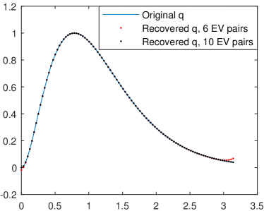
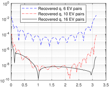
Figure 1: On the left: exact (blue line), recovered from 6 eigenvalue pairs (red dots) and recovered from 10 eigenvalue pairs (black dots) potential $q_{1}$ from Subsection 4.1. On the right: absolute error of the recovered potential, 6, 10 or 16 eigenvalue pairs were used.

On Figure 2 we present the potential $q_{2}$ recovered from 40 and 201 eigenvalue pairs. For 40 eigenvalue pairs the potential $q$ was obtained with $L_{1}(0,\pi)$ error of $4.4\cdot 10^{-2}$, the constants $h$ and $H$ were obtained with the errors of $0.017$ and $0.024$. For 201 eigenvalue pairs, with $1.2\cdot 10^{-2}$, $0.011$ and $0.014$, respectively.

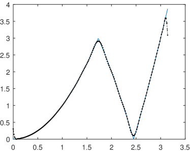
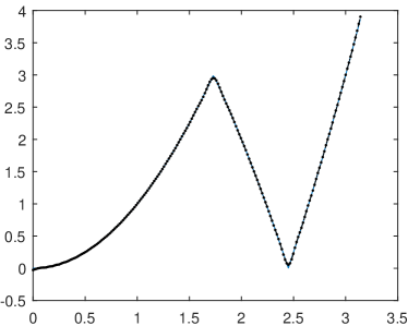
Figure 2: On the left: exact (blue line) and recovered from 40 eigenvalue pairs (black dots); on the right: exact (blue line) and recovered from 201 eigenvalue pairs (black dots) potential $q_{2}$ from Subsection 4.1.

On Figure 3 we present the potential $q_{3}$ recovered from 30 and 201 eigenvalue pairs. While for 30 eigenvalue pairs the algorithm failed near the interval endpoints, inside the interval $(0.5,\pi-0.5)$ the result is acceptable. For 201 eigenvalue pairs the algorithm was able to recover both potential and boundary parameters $h$ and $H$, $L_{1}$ error of the potential was $0.24$, absolute errors of the boundary parameters were $0.0076$ and $0.029$, respectively.

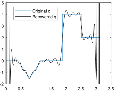
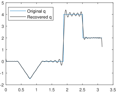
Figure 3: On the left: exact (blue line) and recovered from 30 eigenvalue pairs (black dots); on the right: exact (blue line) and recovered from 201 eigenvalue pairs (black dots) potential $q_{3}$ from Subsection 4.1.

4.2 Inverse problems with known parts of several spectra

As it is stated in [9], “Two-thirds of the spectra of three spectral problems uniquely determine $q$.” In this subsection we numerically illustrate the solution of such inverse problems.

To illustrate the performance of the algorithm we considered two potentials, the same smooth potential $q_{1}$ and the following potential, possessing a discontinuous second derivative $q_{4}(x)=\int_{0}^{x}q_{2}(s)\,ds$, where $q_{1}$ and $q_{2}$ were introduced in Subsection 4.1. We took $H=2$ and $h\in\{1,2,3\}$, and eigenvalues indexed $0,1,3,4,6,7,\ldots$ from the first spectrum, $0,2,3,5,6,8,9,\ldots$ from the second spectrum and $1,2,4,5,7,8,\ldots$ from the third spectrum.

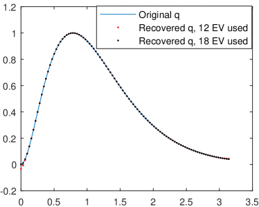
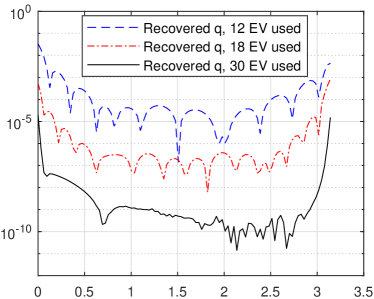
Figure 4: On the left: exact (blue line), recovered from 12 eigenvalues (red dots) and recovered from 18 eigenvalues (black dots) potential $q_{1}$ from Subsection 4.2. On the right: absolute error of the recovered potential, 12, 18 or 30 eigenvalues were used.

On Figure 4 we present the recovered potential $q_{1}$ and its absolute error. The absolute error rapidly decreases with more eigenvalues used and stabilizes at 24 eigenvalues (8 from each spectra). $L_{1}$ error of the recovered $q_{1}$ was $3.9\cdot 10^{-7}$, the parameter $H$ had an absolute error of $3.1\cdot 10^{-7}$.

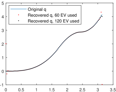
Figure 5: On the left: exact (blue line), recovered from 60 eigenvalues (red dots) and recovered from 120 eigenvalues (black dots) potential $q_{4}$ from Subsection 4.2. On the right: absolute error of the recovered potential, 60 or 120 eigenvalues were used.

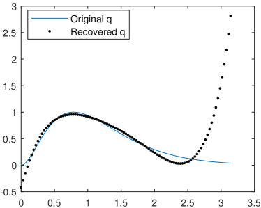
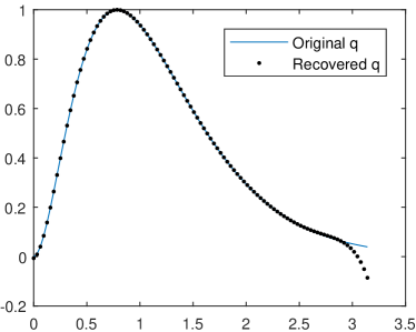
Figure 6: Exact potential $q_{1}$ from Subsection 4.2 (blue line) and recovered one (black dots). On the left: recovered from 10 eigenvalues $\lambda_{0}(h)$, $h\in\{0,1,2,3,4,5,10,20,50,100\}$, on the right: recovered from 30 eigenvalues $\lambda_{0}(h),\lambda_{1}(h),\lambda_{2}(h)$, $h\in\{0,1,2,3,4,5,10,20,50,100\}$.

On Figure 5 we present the recovered potential $q_{4}$ and its absolute error. In this case the potential is of finite smoothness, so the algorithm converges slowly. With 120 eigenvalues (40 from each spectrum) we obtained the following errors: $L_{1}$ error of the potential was $3.7\cdot 10^{-3}$ and the error of the parameter $H$ was $1.5\cdot 10^{-3}$.

In [7, Section 3.14] the following inverse problem was considered. Suppose that the first eigenvalue is known for spectral problems having the same potential but different boundary conditions at $x=0$. From countably many values the potential can be recovered uniquely. However, if only finitely many values are given, the situation changes. The corresponding numerical problem is extremely ill-posed, so the method from [34] was not able to solve it, and the modification from [7] was able to recover only the general shape of the potential.

We tried the proposed algorithm on this problem. For a numerical example we took the potential $q_{1}$ from Subsection 4.1, $H=0$ and $h\in\{0,1,2,3,4,5,10,20,50,100\}$. On Figure 6, left plot, we present the recovered potential. The algorithm failed, it is a case of very small interval for $z_{k}$. And the result does not improve if we take more values of the parameter $h$. However the situation greatly improves if instead of 1 eigenvalue for each spectral problem we take several. On Figure 6, right plot, we present the recovered potential for the inverse problem when the first 3 eigenvalues were taken from each spectrum.

4.3 Partially known potential

In this subsection we illustrate the performance of the proposed method applied to solution of inverse problems with a partially known potential. For comparison we have taken two potentials from [21], a smooth potential $q_{5}(x)=\frac{e^{x}-x^{2}}{12}$ and a non-smooth continuous potential $q_{2}(x)=|3-|x^{2}-3||$. The potentials are known on $[0,\pi/2]$, hence one spectrum is necessary to recover the potential. While in [21] the Dirichlet boundary conditions are considered, we decided to take mixed boundary conditions with $h=1$ and $H=2$ for both potentials.

To solve the inverse problem we followed the idea presented in Subsubsection 2.2.3: solve the Cauchy problems with initial data $v(\rho_{n},0)=1$, $v^{\prime}(\rho_{n},0)=h$ on the segment $[0,\pi/2]$, compute the values of the Weyl-Titchmarsh $m$-function

$$m(\pi/2,\rho_{n}^{2})=\frac{v^{\prime}(\rho_{n},\pi/2)}{v(\rho_{n},\pi/2)},$$

transform them to the Weyl function $M$ using (2.11). After a simple rescaling we get Problem 2.4.

For the numerical example 40 eigenvalues with 1 missing eigenvalue were considered in [21]. For the potential $q_{5}$ we similarly considered 40 eigenvalues, but with 2 eigenvalues missing: $\lambda_{10}$ and $\lambda_{35}$. For the potential $q_{2}$ one eigenvalue $\lambda_{35}$ was missing. We would like to emphasize that we used the proposed method “as is”, without recovering missing eigenvalues (which is impossible, since the algorithm has no information if the points $z_{n}$ correspond to any eigenvalues).

On Figures 7 and 8 we present the recovered potentials and their absolute errors. One can appreciate an especially excellent accuracy in the case of a smooth potential.

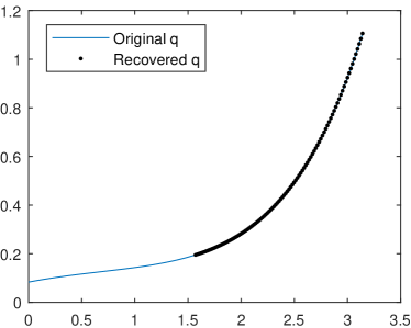
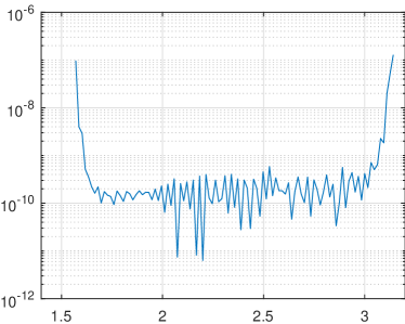
Figure 7: On the left: exact (blue line) and recovered (black dots) potential $q_{5}$ from Subsection 4.3. On the right: absolute error of the recovered potential. Eigenvalues $\{\lambda_{n}\}_{n=0}^{39}\setminus\{\lambda_{10},\lambda_{35}\}$ were used. The error of the recovered parameter $H$ is $5.0\cdot 10^{-10}$, and the $L_{1}$ error of the recovered potential is $3.0\cdot 10^{-9}$.

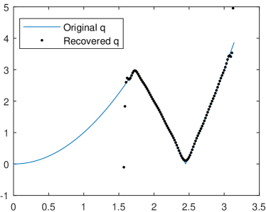
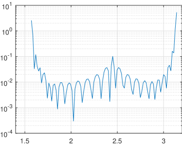
Figure 8: On the left: exact (blue line) and recovered (black dots) potential $q_{2}$ from Subsection 4.3. On the right: absolute error of the recovered potential. Eigenvalues $\{\lambda_{n}\}_{n=0}^{39}\setminus\{\lambda_{35}\}$ were used. The error of the recovered parameter $H$ is $2.5\cdot 10^{-2}$, and the $L_{1}$ error of the recovered potential is $0.11$.

4.4 Recovery of the potential from values of the Weyl function: complex points $z_{n}$ and some problematic choices

The proposed algorithm works even when the numbers $z_{n}$ are complex (however for numerical stability the imaginary parts should be relatively small comparing to the real parts). For illustration we considered the potential $q_{1}$ from Subsection 4.1, $h=1$, $H=2$ and the following sets of points

$$z_{n}^{(k)}=\left(\frac{1}{5}+\frac{n}{2}+k\cdot i\right)^{2},\qquad 0\leq n\leq 40,\ k\in\{0,1,2\}.$$ (4.1)

The obtained results are presented on Figure 9, left plot. The algorithm was able to recover both the potential and the boundary conditions, however the accuracy decreases when the points are taken farther from the real line.

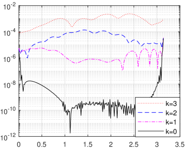
Figure 9: Absolute errors of the recovered potential $q_{1}$ from Subsection 4.4. On the left: using the points (4.1) with different values of $k$. On the right: using the points shown on the legend, $0\leq n\leq 40$.

It should be mentioned that the proposed algorithm may fail for some particular choices of the points $z_{n}$ even for nice potentials. We considered the same problem and the following set of points

$$y_{n}^{(1)}=\left(\frac{1}{4}+\frac{n}{2}\right)^{2},\qquad 0\leq n\leq 40.$$

The truncated system (3.11) was not ill conditioned, but its solution was nowhere close to the exact one and the situation does not improve when taking more or less unknowns. For example, for 9 unknowns $\xi_{0},\ldots,\xi_{8}$ the parameter $h=\omega-\omega_{2}$ resulted to be $0.7999$ instead of $1$. The best value was achieved for 10 unknowns and that was $0.8677$. On Figure 9, right plot we present the absolute error of the recovered potential in comparison with those recovered using a very close set of points

$$y_{n}^{(2)}=\left(0.249+\frac{n}{2}\right)^{2},\qquad 0\leq n\leq 40.$$

For the latter choice of points, the recovered parameter $h$ resulted to be $0.999997$ and the potential was recovered to 5 extra decimal digits. It should be noted that the sets $\{y_{n}^{(1)}\}_{n=0}^{\infty}$ and $\{y_{n}^{(2)}\}_{n=0}^{\infty}$ do not satisfy neither the condition (2.15) nor the condition from [20], so any behavior can be expected for finite subsets. And the set $\{y_{n}^{(1)}\}_{n=0}^{\infty}$ is, in some sense, the worst possible since the points $y_{n}^{(1)}$ are the most distant from any eigenvalue asymptotics (numbers close either to integers or integers plus one half). The situation changes completely if we consider the set $\{0\}\cup\{y_{n}^{(1)}\}_{n=0}^{\infty}$. This set satisfies the condition (2.15), and the proposed method works for it without any problem, see Figure 9, right plot. The recovered parameter $h$ was $0.9999999991$.

5 Conclusions

A direct method for recovering the Sturm-Liouville problem from the Weyl-Titchmarsh function given on a countable set of points is developed, which leads to an efficient numerical algorithm for solving a variety of inverse Sturm-Liouville problems. The main role in the proposed approach is played by the coefficients of the Fourier-Legendre series expansion of the transmutation operator integral kernel. We show how the given spectral data lead to an infinite system of linear algebraic equations for the coefficients, and the crucial observation is that for recovering the potential it is sufficient to find the first coefficient only. In practical terms this observation translates into the fact that very few equations in the truncated system are enough for solving the inverse Sturm-Liouville problem.

The method is simple, direct and accurate. Its limitations are all related to a possible insufficiency of the input data. A too reduced number of eigendata or a special choice of points at which the Weyl function is given may lead to inaccurate results, as we illustrate by numerical examples.

References

- [1] M. Abramovitz and I. A. Stegun, Handbook of mathematical functions, New York: Dover, 1972.
- [2] F. V. Atkinson, Discrete and continuous boundary problems, New York: Academic Press, 1964.
- [3] A. R. Barnett, The calculation of spherical Bessel and Coulomb functions, in Computational Atomic Physics, Electron and Positron Collisions with Atoms and Ions, Berlin: Springer-Verlag, 1996, 181–202.
- [4] N. P. Bondarenko, Inverse Sturm-Liouville problem with analytical functions in the boundary condition, Open Mathematics 18 (2020), 512–528.
- [5] N. P. Bondarenko, Solvability and stability of the inverse Sturm–Liouville problem with analytical functions in the boundary condition, Math. Meth. Appl. Sci. 43 (2020), 7009–7021.
- [6] H. Campos, V. V. Kravchenko and S. M. Torba, Transmutations, L-bases and complete families of solutions of the stationary Schrödinger equation in the plane, J. Math. Anal. Appl. 389 (2012), no. 2, 1222–1238.
- [7] Kh. Chadan, D. Colton, L. Päivärinta and W. Rundell, An introduction to inverse scattering and inverse spectral problems. SIAM, Philadelphia, 1997.
- [8] K. Chadan and P. C. Sabatier, Inverse problems in quantum scattering theory. Second edition, Springer-Verlag, New York, 1989.
- [9] F. Gesztesy, R. del Rio and B. Simon, Inverse spectral analysis with partial information on the potential, III. Updating boundary conditions, Internat. Math. Research Notices 15 (1997), 751–758.
- [10] F. Gesztesy and B. Simon, A new approach to inverse spectral theory II. General real potentials and the connection to the spectral measure, Ann. of Math. 152 (2000), 593–643.
- [11] F. Gesztesy and B. Simon, Inverse spectral analysis with partial information on the potential, II. The case of discrete spectrum, Trans. Amer. Math. Soc. 352 (2000), 2765–2787.
- [12] E. Gillman and H. R. Fiebig, Accurate recursive generation of spherical Bessel and Neumann functions for a large range of indices, Comput. Phys. 2 (1988), 62–72.
- [13] G. M. L. Gladwell, Inverse problems in vibration – II, Appl. Mech. Rev. 49(10S) (1996), S25–S34.
- [14] G. M. L. Gladwell, Inverse problems in vibration. Second edition, Kluwer Academic Publishers, Dordrecht, 2005.
- [15] K. Gou and Z. Chen, Inverse Sturm-Liouville problems and their biomedical engineering applications, JSM Math. Stat. 2 (2015), 1008.
- [16] T. N. Harutyunyan and A. M. Tonoyan, Some properties of the kernel of a transmutation operator, 2021, to appear.
- [17] H. Hochstadt, The inverse Sturm–Liouville problem, Comm. Pure Appl. Math., 26 (1973), 715–729.
- [18] H. Hochstadt and B. Lieberman, An inverse Sturm-Liouville problem with mixed given data, SIAM J. Appl. Math. 34 (1978), 676–680.
- [19] M. Horváth, On the inverse spectral theory of Schrödinger and Dirac operators, Trans. Amer. Math. Soc. 353 (2001), 4155–4171.
- [20] M. Horváth, Inverse spectral problems and closed exponential systems, Ann. of Math. 162 (2005), 885–918.
- [21] A. Kammanee and C. Böckmann, Determination of partially known Sturm–Liouville potentials, Appl. Math. Comput. 204 (2008) 928–937.
- [22] K. V. Khmelnytskaya, V. V. Kravchenko and S. M. Torba, A representation of the transmutation kernels for the Schrödinger operator in terms of eigenfunctions and applications, Appl. Math. Comput. 353 (2019), 274–281.
- [23] K. V. Khmelnytskaya and T. V. Torchynska, Reconstruction of potentials in quantum dots and other small symmetric structures, Math. Methods Appl. Sci. 33 (2010), 469–472.
- [24] V. V. Kravchenko, On a method for solving the inverse Sturm–Liouville problem, J. Inverse Ill-posed Probl. 27 (2019), 401–407.
- [25] V. V. Kravchenko, Direct and inverse Sturm-Liouville problems: A method of solution, Birkhäuser, Cham, 2020.
- [26] V. V. Kravchenko, L. J. Navarro and S. M. Torba, Representation of solutions to the one-dimensional Schrödinger equation in terms of Neumann series of Bessel functions, Appl. Math. Comput. 314 (2017), 173–192.
- [27] V. V. Kravchenko and S. M. Torba, A Neumann series of Bessel functions representation for solutions of Sturm-Liouville equations, Calcolo 55 (2018), article 11, 23pp.
- [28] V. V. Kravchenko and S. M. Torba, A direct method for solving inverse Sturm-Liouville problems, Inverse Probl. 37 (2021), 015015 (32pp).
- [29] B. M. Levitan, Inverse Sturm-Liouville problems, VSP, Zeist, 1987.
- [30] V. A. Marchenko, Some questions on one-dimensional linear second order differential operators, Transactions of Moscow Math. Soc., 1 (1952), 327–420.
- [31] V. A. Marchenko, Sturm-Liouville operators and applications: revised edition, AMS Chelsea Publishing, 2011.
- [32] M. Neher, Enclosing solutions of an inverse Sturm-Liouville problem with finite data, Computing 53 (1994), 379–395.
- [33] V. Pivovarchik, An inverse problem by eigenvalues of four spectra, J. Math. Anal. Appl. 396 (2012) 715–723.
- [34] W. Rundell and P. E. Sacks, Reconstruction techniques for classical inverse Sturm–Liouville problems, Math. Comput. 58 (1992), 161–183.
- [35] A. M. Savchuk, Reconstruction of the potential of the Sturm–Liouville operator from a finite set of eigenvalues and normalizing constants, Math. Notes 99 (2016), 715–728.
- [36] E. L. Shishkina and S. M. Sitnik, Transmutations, singular and fractional differential equations with applications to mathematical physics, Elsevier, Amsterdam, 2020.
- [37] A. M. Savchuk and A. A. Shkalikov, Recovering of a potential of the Sturm-Liouville problem from finite sets of spectral data, in Spectral Theory and Differential Equations, Amer. Math. Soc. Transl. Ser. 2, 233 (2014), 211–224.
- [38] A. A. Shkalikov, Boundary problems for ordinary differential equations with parameter in the boundary conditions, J. Sov. Math. 33 (1986), 1311–1342.
- [39] B. Simon, A new approach to inverse spectral theory I. Fundamental formalism, Ann. of Math. 150 (1999), 1029–1057.
- [40] A. O. Vatulyan, Inverse problems of solid mechanics, Fizmatlit, Moscow, 2007 (in Russian).
- [41] C. F. Yang, N. P. Bondarenko and X. C. Xu, An inverse problem for the Sturm-Liouville pencil with arbitrary entire functions in the boundary condition, Inverse Probl. Imag. 14 (2020), 153–169.
- [42] V. A. Yurko, Introduction to the theory of inverse spectral problems, Fizmatlit, Moscow, 2007 (in Russian).