Breaking the Deadly Triad with a Target Network

Abstract

The deadly triad refers to the instability of a reinforcement learning algorithm when it employs off-policy learning, function approximation, and bootstrapping simultaneously. In this paper, we investigate the target network as a tool for breaking the deadly triad, providing theoretical support for the conventional wisdom that a target network stabilizes training. We first propose and analyze a novel target network update rule which augments the commonly used Polyak-averaging style update with two projections. We then apply the target network and ridge regularization in several divergent algorithms and show their convergence to regularized TD fixed points. Those algorithms are off-policy with linear function approximation and bootstrapping, spanning both policy evaluation and control, as well as both discounted and average-reward settings. In particular, we provide the first convergent linear $Q$-learning algorithms under nonrestrictive and changing behavior policies without bi-level optimization.

lb sz yh

1 Introduction

The deadly triad (see, e.g., Chapter 11.3 of Sutton & Barto (2018)) refers to the instability of a value-based reinforcement learning (RL, Sutton & Barto (2018)) algorithm when it employs off-policy learning, function approximation, and bootstrapping simultaneously. Different from on-policy methods, where the policy of interest is executed for data collection, off-policy methods execute a different policy for data collection, which is usually safer (Dulac-Arnold et al., 2019) and more data efficient (Lin, 1992; Sutton et al., 2011). Function approximation methods use parameterized functions, instead of a look-up table, to represent quantities of interest, which usually cope better with large-scale problems (Mnih et al., 2015; Silver et al., 2016). Bootstrapping methods construct update targets for an estimate by using the estimate itself recursively, which usually has lower variance than Monte Carlo methods (Sutton, 1988). However, when an algorithm employs all those three preferred ingredients (off-policy learning, function approximation, and bootstrapping) simultaneously, there is usually no guarantee that the resulting algorithm is well behaved and the value estimates can easily diverge (see, e.g., Baird (1995); Tsitsiklis & Van Roy (1997); Zhang et al. (2021)), yielding the notorious deadly triad.

An example of the deadly triad is $Q$-learning (Watkins & Dayan, 1992) with linear function approximation, whose divergence is well documented in Baird (1995). However, Deep-$Q$-Networks (DQN, Mnih et al. (2015)), a combination of $Q$-learning and deep neural network function approximation, has enjoyed great empirical success. One major improvement of DQN over linear $Q$-learning is the use of a target network, a copy of the neural network function approximator (the main network) that is periodically synchronized with the main network. Importantly, the bootstrapping target in DQN is computed via the target network instead of the main network. As the target network changes slowly, it provides a stable bootstrapping target which in turn stabilizes the training of DQN. Instead of the periodical synchronization, Lillicrap et al. (2015) propose a Polyak-averaging style target network update, which has also enjoyed great empirical success (Fujimoto et al., 2018; Haarnoja et al., 2018).

Inspired by the empirical success of the target network in RL with deep networks, in this paper, we theoretically investigate the target network as a tool for breaking the deadly triad. We consider a two-timescale framework, where the main network is updated faster than the target network. By using a target network to construct the bootstrapping target, the main network update becomes least squares regression. After adding ridge regularization (Tikhonov et al., 2013) to this least squares problem, we show convergence for both the target and main networks.

Our main contributions are twofold. First, we propose a novel target network update rule augmenting the Polyak-averaging style update with two projections. The balls for the projections are usually large so most times they are just identity mapping. However, those two projections offer significant theoretical advantages making it possible to analyze where the target network converges to (Section 3). Second, we apply the target network in various existing divergent algorithms and show their convergence to regularized TD (Sutton, 1988) fixed points. Those algorithms are off-policy algorithms with linear function approximation and bootstrapping, spanning both policy evaluation and control, as well as both discounted and average-reward settings. In particular, we provide the first convergent linear $Q$-learning algorithms under nonrestrictive and changing behavior policies without bi-level optimization, for both discounted and average-reward settings.

2 Background

Let $M$ be a real positive definite matrix and $x$ be a vector, we use $\norm{x}_{M}\doteq\sqrt{x^{\top}Mx}$ to denote the norm induced by $M$ and $\norm{\cdot}_{M}$ to denote the corresponding induced matrix norm. When $M$ is the identity matrix $I$, we ignore the subscript $I$ for simplicity. We use vectors and functions interchangeably when it does not cause confusion, e.g., given $f:\mathcal{X}\to\mathbb{R}$, we also use $f$ to denote the corresponding vector in $\mathbb{R}^{|\mathcal{X}|}$. All vectors are column vectors. We use 1 to denote an all one vector, whose dimension can be deduced from the context. 0 is similarly defined.

We consider an infinite horizon Markov Decision Process (MDP, see, e.g., Puterman (2014)) consisting of a finite state space $\mathcal{S}$, a finite action space $\mathcal{A}$, a transition kernel $p:\mathcal{S}\times\mathcal{S}\times\mathcal{A}\to[0,1]$, and a reward function $r:\mathcal{S}\times\mathcal{A}\to\mathbb{R}$. At time step $t$, an agent at a state $S_{t}$ executes an action $A_{t}\sim\pi(\cdot|S_{t})$, where $\pi:\mathcal{A}\times\mathcal{S}\to[0,1]$ is the policy followed by the agent. The agent then receives a reward $R_{t+1}\doteq r(S_{t},A_{t})$ and proceeds to a new state $S_{t+1}\sim p(\cdot|S_{t},A_{t})$.

In the discounted setting, we consider a discount factor $\gamma\in[0,1)$ and define the return at time step $t$ as $G_{t}\doteq\sum_{i=1}^{\infty}\gamma^{i-1}R_{t+i}$, which allows us to define the action-value function $q_{\pi}(s,a)\doteq\mathbb{E}_{\pi,p}[G_{t}|S_{t}=s,A_{t}=a]$. The action-value function $q_{\pi}$ is the unique fixed point of the Bellman operator ${\mathcal{T}}_{\pi}$, i.e., $q_{\pi}={\mathcal{T}}_{\pi}q_{\pi}\doteq r+\gamma P_{\pi}q_{\pi}$, where $P_{\pi}\in\mathbb{R}^{{|\mathcal{S}||\mathcal{A}|}\times{|\mathcal{S}||\mathcal{A}|}}$ is the transition matrix, i.e., $P_{\pi}((s,a),(s^{\prime},a^{\prime}))\doteq\sum_{a}p(s^{\prime}|s,a)\pi(a^{\prime}|s^{\prime})$.

In the average-reward setting, we assume:

Assumption 2.1.

The chain induced by $\pi$ is ergodic.

This allows us to define the reward rate
$\bar{r}_{\pi}\doteq\lim_{T\to\infty}\frac{1}{T}\sum_{t=1}^{T}\mathbb{E}[R_{t}|p,\pi]$. The differential action-value function $\bar{q}_{\pi}(s,a)$ is defined as

$$\textstyle{\lim_{T\to\infty}\sum_{t=0}^{T}\mathbb{E}_{\pi,p}[r(S_{t},A_{t})-\bar{r}_{\pi}|S_{0}=s,A_{0}=a]}.$$ (1)

The differential Bellman equation is

$$\bar{q}=r-\bar{r}{\textbf{1}}+P_{\pi}\bar{q},$$ (2)

where $\bar{q}\in\mathbb{R}^{|\mathcal{S}||\mathcal{A}|}$ and $\bar{r}\in\mathbb{R}$ are free variables. It is well known that all solutions to (2) form a set $\quantity{(\bar{q},\bar{r})\mid\bar{r}=\bar{r}_{\pi},\bar{q}=q_{\pi}+c{\textbf{1}},c\in\mathbb{R}}$ (Puterman, 2014).

The policy evaluation problem refers to estimating $q_{\pi}$ or $(\bar{q}_{\pi},\bar{r}_{\pi})$. The control problem refers to finding a policy $\pi$ maximizing $q_{\pi}(s,a)$ for each $(s,a)$ or maximizing $\bar{r}_{\pi}$. With linear function approximation, we approximate $q_{\pi}(s,a)$ or $\bar{q}_{\pi}(s,a)$ with $x(s,a)^{\top}w$, where $x:\mathcal{S}\times\mathcal{A}\to\mathbb{R}^{K}$ is a feature mapping and $w\in\mathbb{R}^{K}$ is the learnable parameter. We use $X\in\mathbb{R}^{{|\mathcal{S}||\mathcal{A}|}\times K}$ to denote the feature matrix, each row of which is $x(s,a)^{\top}$, and assume:

Assumption 2.2.

$X$ has linearly independent columns.

In the average-reward setting, we use an additional parameter $\bar{r}\in\mathbb{R}$ to approximate $\bar{r}_{\pi}$. In the off-policy learning setting, the data for policy evaluation or control is collected by executing a policy $\mu$ (behavior policy) in the MDP, which is different from $\pi$ (target policy). In the rest of the paper, we consider the off-policy linear function approximation setting thus always assume $A_{t}\sim\mu(\cdot|S_{t})$. We use as shorthand $x_{t}\doteq x(S_{t},A_{t}),\bar{x}_{t}\doteq\sum_{a}\pi(a|S_{t})x(S_{t},a)$.

Policy Evaluation. In the discounted setting, similar to Temporal Difference Learning (TD, Sutton (1988)), one can use Off-Policy Expected SARSA to estimate $q_{\pi}$, which updates $w$ as

$$\delta_{t} \leftarrow R_{t+1}+\gamma\bar{x}_{t+1}^{\top}w_{t}-x_{t}^{\top}w_{t},$$ (3)

$$w_{t+1} \leftarrow w_{t}+\alpha_{t}\delta_{t}x_{t},$$ (4)

where $\quantity{\alpha_{t}}$ are learning rates. In the average-reward setting, (2) implies that $\bar{r}_{\pi}=d^{\top}(r+P_{\pi}\bar{q}_{\pi}-\bar{q}_{\pi})$ holds for any probability distribution $d$. In particular, it holds for $d=d_{\mu}$. Consequently, to estimate $\bar{q}_{\pi}$ and $\bar{r}_{\pi}$, Wan et al. (2020); Zhang et al. (2021) update $w$ and $\bar{r}$ as

$$w_{t+1} \leftarrow w_{t}+\alpha_{t}(R_{t+1}-\bar{r}_{t}+\bar{x}_{t+1}^{\top}w_{t}-x_{t}^{\top}w_{t})x_{t},$$ (5)

$$\bar{r}_{t+1} \leftarrow\bar{r}_{t}+\alpha_{t}(R_{t+1}+\bar{x}_{t+1}^{\top}w_{t}-x_{t}^{\top}w_{t}-\bar{r}_{t}).$$ (6)

Unfortunately, both (4) and (6) can possibly diverge (see, e.g., Tsitsiklis & Van Roy (1997); Zhang et al. (2021)), which exemplifies the deadly triad in discounted and average-reward settings respectively.

Control. In the discounted setting, $Q$-learning with linear function approximation yields

$$\delta_{t} \leftarrow R_{t+1}+\gamma\max_{a^{\prime}}x(S_{t+1},a^{\prime})^{\top}w_{t}-x_{t}^{\top}w_{t},$$ (7)

$$w_{t+1} \leftarrow w_{t}+\alpha_{t}\delta_{t}x_{t}.$$ (8)

In the average-reward setting, Differential $Q$-learning (Wan et al., 2020) with linear function approximation yields

$$\delta_{t} \leftarrow R_{t+1}-\bar{r}_{t}+\gamma\max_{a^{\prime}}x(S_{t+1},a^{\prime})^{\top}w_{t}-x_{t}^{\top}w_{t},$$ (9)

$$w_{t+1} \leftarrow w_{t}+\alpha_{t}\delta_{t}x_{t},\quad\bar{r}_{t+1}\leftarrow\bar{r}_{t}+\alpha_{t}\delta_{t}.$$ (10)

Unfortunately, both (8) and (10) can possibly diverge as well (see, e.g., Baird (1995); Zhang et al. (2021)), exemplifying the deadly triad again.

Motivated by the empirical success of the target network in deep RL, one can apply the target network in the linear function approximation setting. For example, using a target network in (8) yields

$$\delta_{t} \leftarrow R_{t+1}+\gamma\max_{a^{\prime}}x(S_{t+1},a^{\prime})^{\top}\theta_{t}-x_{t}^{\top}w_{t},$$ (11)

$$w_{t+1} \leftarrow w_{t}+\alpha_{t}\delta_{t}x_{t},$$ (12)

$$\theta_{t+1} \leftarrow\theta_{t}+\beta_{t}(w_{t}-\theta_{t}),$$ (13)

where $\theta$ denotes the target network, $\quantity{\beta_{t}}$ are learning rates, and we consider the Polyak-averaging style target network update. The convergence of (12) and (13), however, remains unknown. Besides target networks, regularization has also been widely used in deep RL, e.g., Mnih et al. (2015) consider a Huber loss instead of a mean-squared loss; Lillicrap et al. (2015) consider $\ell_{2}$ weight decay in updating $Q$-values.

3 Analysis of the Target Network

In Sections 4 & 5, we consider the merits of using a target network in several linear RL algorithms (e.g., (4) (6) (8) (10)). To this end, in this section, we start by proposing and analyzing a novel target network update rule:

$$\theta_{t+1}\doteq\Gamma_{B_{1}}\big{(}\theta_{t}+\beta_{t}(\Gamma_{B_{2}}(w_{t})-\theta_{t})\big{)}.$$ (14)

In (14), $w$ denotes the main network and $\theta$ denotes the target network. $\Gamma_{B_{1}}:\mathbb{R}^{K}\to\mathbb{R}^{K}$ is a projection to the ball $B_{1}\doteq\quantity{x\in\mathbb{R}^{K}\mid\norm{x}\leq R_{B_{1}}}$, i.e.,

$$\textstyle{\Gamma_{B_{1}}(x)\doteq x\mathbb{I}_{\norm{x}\leq R_{B_{1}}}+({R_{B_{1}}x}/{\norm{x}})\mathbb{I}_{\norm{x}>R_{B_{1}}}},$$ (15)

where $\mathbb{I}$ is the indicator function. $\Gamma_{B_{2}}$ is a projection onto the ball $B_{2}$ with a radius $R_{B_{2}}$. We make the following assumption about the learning rates:

Assumption 3.1.

$\quantity{\beta_{t}}$ is a deterministic positive nonincreasing sequence satisfying $\sum_{t}\beta_{t}=\infty,\sum_{t}\beta_{t}^{2}<\infty$.

While (14) specifies only how $\theta$ is updated, we assume $w$ is updated such that $w$ can track $\theta$ in the sense that

Assumption 3.2.

There exists $w^{*}:\mathbb{R}^{K}\to\mathbb{R}^{K}$ such that $\lim_{t\to\infty}\norm{w_{t}-w^{*}(\theta_{t})}=0$ almost surely.

After making some additional assumptions on $w^{*}$, we arrive at our general convergent results.

Assumption 3.3.

$\sup_{\theta}\norm{w^{*}(\theta)}<R_{B_{2}}<R_{B_{1}}<\infty$.

Assumption 3.4.

$w^{*}$ is a contraction mapping w.r.t. $\norm{\cdot}$.

Theorem 1.

(Convergence of Target Network) Under Assumptions 3.1-3.4, the iterate $\quantity{\theta_{t}}$ generated by (14) satisfies

$$\textstyle{\lim_{t\to\infty}w_{t}=\lim_{t\to\infty}\theta_{t}=\theta^{*}}\mbox{\quad almost surely,\quad}$$ (16)

where $\theta^{*}$ is the unique fixed point of $w^{*}(\cdot)$.

Assumptions 3.2 - 3.4 are assumed only for now. Once the concrete update rules for $w$ are specified in the algorithms in Sections 4 & 5, we will prove that those assumptions indeed hold. Assumption 3.2 is expected to hold because we will later require that the target network to be updated much slower than the main network. Consequently, the update of the main network will become a standard least-square regression, whose solution $w^{*}$ usually exists. Assumption 3.4 is expected to hold becuase we will later apply ridge regularization to the least-square regression. Consequently, its solution $w^{*}$ will not change too fast w.r.t. the change of the regression target.

The target network update (14) is the same as that in (13) except for the two projections, where the first projection $\Gamma_{B_{1}}$ is standard in optimization literature. The second projection $\Gamma_{B_{2}}$, however, appears novel and plays a crucial role in our analysis. First, if we have only $\Gamma_{B_{1}}$, the iterate $\quantity{\theta_{t}}$ would converge to the invariant set of the ODE

$$\textstyle{\derivative{t}\theta(t)=w^{*}(\theta(t))-\theta(t)+\zeta(t)},$$ (17)

where $\zeta(t)$ is a reflection term that moves $\theta(t)$ back to $B_{1}$ when $\theta(t)$ becomes too large (see, e.g., Section 5 of Kushner & Yin (2003)). Due to this reflection term, it is possible that $\theta(t)$ visits the boundary of $B_{1}$ infinitely often. It thus becomes unclear what the invariant set of (17) is even if $w^{*}$ is contractive. By introducing the second projection $\Gamma_{B_{2}}$ and ensuring $R_{B_{1}}>R_{B_{2}}$, we are able to remove the reflection term and show that the iterate $\quantity{\theta_{t}}$ tracks the ODE

$$\textstyle{\derivative{t}\theta(t)=w^{*}(\theta(t))-\theta(t)},$$ (18)

whose invariant set is a singleton $\quantity{\theta^{*}}$ when Assumption 3.4 holds. See the proof of Theorem 1 in Section A.1 based on the ODE approach (Kushner & Yin, 2003; Borkar, 2009) for more details. Second, to ensure the main network tracks the target network in the sense of Assumption 3.2 in our applications in Sections 4 & 5, it is crucial that the target network changes sufficiently slowly in the following sense:

Lemma 1.

$\norm{\theta_{t+1}-\theta_{t}}\leq\beta_{t}C_{0}$ for some constant $C_{0}>0$.

Lemma 1 would not be feasible without the second projection $\Gamma_{B_{2}}$ and we defer its proof to Section A.2

In Sections 4 & 5, we provide several applications of Theorem 1 in both discounted and average-reward settings, for both policy evaluation and control. We consider a two-timescale framework, where the target network is updated more slowly than the main network. Let $\quantity{\alpha_{t}}$ be the learning rates for updating the main network $w$; we assume

Assumption 3.5.

$\quantity{\alpha_{t}}$ is a deterministic positive nonincreasing sequence satisfying $\sum_{t}\alpha_{t}=\infty,\sum_{t}\alpha_{t}^{2}<\infty$. Further, for some $d>0$, $\sum_{t}(\beta_{t}/\alpha_{t})^{d}<\infty$.

4 Application to Off-Policy Policy Evaluation

In this paper, we consider estimating the action-value $q_{\pi}$ instead of the state-value $v_{\pi}$ for unifying notations of policy evaluation and control. The algorithms for estimating $v_{\pi}$ are straightforward up to change of notations and introduction of importance sampling ratios.

Discounted Setting. Using a target network for bootstrapping in (4) yields

$$w_{t+1}\leftarrow w_{t}+\alpha_{t}(R_{t+1}+\gamma\bar{x}_{t+1}^{\top}\theta_{t}-x_{t}^{\top}w_{t})x_{t}.$$ (19)

As $\theta_{t}$ is quasi-static for $w_{t}$ (Lemma 1 and Assumption 3.5), this update becomes least squares regression. Motivated by the success of ridge regularization in least squares and the widespread use of weight decay in deep RL, which is essentially ridge regularization, we add ridge regularization to this least squares, yielding $Q$-evaluation with a Target Network (Algorithm 1).

Algorithm 1 $Q$-evaluation with a Target Network

  INPUT: $\eta>0,R_{B_{1}}>R_{B_{2}}>0$

  Initialize $\theta_{0}\in B_{1}$ and $S_{0}$

  Sample $A_{0}\sim\mu(\cdot|S_{0})$

  for $t=0,1,\dots$ do

     Execute $A_{t}$, get $R_{t+1}$ and $S_{t+1}$

     Sample $A_{t+1}\sim\mu(\cdot|S_{t+1})$

     $\bar{x}_{t+1}\doteq\sum_{a^{\prime}}\pi(a^{\prime}|S_{t+1})x(S_{t+1},a^{\prime})$

     $\delta_{t}\doteq R_{t+1}+\gamma\bar{x}_{t+1}^{\top}\theta_{t}-x_{t}^{\top}w_{t}$

     $w_{t+1}\doteq w_{t}+\alpha_{t}\delta_{t}x_{t}-\alpha_{t}\eta w_{t}$

     $\theta_{t+1}\doteq\Gamma_{B_{1}}\big{(}\theta_{t}+\beta_{t}(\Gamma_{B_{2}}(w_{t})-\theta_{t})\big{)}$

  end for

Let $A=X^{\top}D_{\mu}(I-\gamma P_{\pi})X,b=X^{\top}D_{\mu}r$, where $D_{\mu}$ is a diagonal matrix whose diagonal entry is $d_{\mu}$, the stationary state-action distribution of the chain induced by $\mu$. Let $\Pi_{D_{\mu}}\doteq X(X^{\top}D_{\mu}X)^{-1}X^{\top}D_{\mu}$ be the projection to the column space of $X$. We have

Assumption 4.1.

The chain in $\mathcal{S}\times\mathcal{A}$ induced by $\mu$ is ergodic.

Theorem 2.

Under Assumptions 2.2, 3.1, 3.5, & 4.1, for any $\xi\in(0,1)$, let $\textstyle{C_{0}\doteq\frac{2(1-\xi)\sqrt{\eta}}{\gamma\norm{P_{\pi}}_{D_{\mu}}},C_{1}\doteq\frac{\norm{r}}{2\xi\sqrt{\eta}}+1}$, then for all $\norm{X}<C_{0},C_{1}<R_{B_{1}},R_{B_{1}}-\xi<R_{B_{2}}<R_{B_{1}}$ the iterate $\quantity{w_{t}}$ generated by Algorithm 1 satisfies

$$\textstyle{\lim_{t\to\infty}w_{t}=w^{*}_{\eta}}\mbox{\quad almost surely,\quad}$$ (20)

where $w^{*}_{\eta}$ is the unique solution of $(A+\eta I)w-b={\textbf{0}}$, and

$$\norm{Xw^{*}_{\eta}-q_{\pi}}$$ (21)

$$\leq \textstyle{(\frac{\sigma_{\max}(X)^{2}}{\sigma_{\min}(X)^{4}\sigma_{\min}(D_{\mu})^{2.5}}\norm{q_{\pi}}\eta+\norm{\Pi_{D_{\mu}}q_{\pi}-q_{\pi}})/\xi},$$ (22)

where $\sigma_{\max}(\cdot),\sigma_{\min}(\cdot)$ denotes the largest and minimum singular values.

We defer the proof to Section A.3. Theorem 2 requires that the balls for projection are sufficiently large, which is completely feasible in practice. Theorem 2 also requires that the feature norm $\norm{X}$ is not too large. Similar assumptions on feature norms also appear in Zou et al. (2019); Du et al. (2019); Chen et al. (2019b); Carvalho et al. (2020); Wang & Zou (2020); Wu et al. (2020) and can be easily achieved by scaling.

The solutions to $Aw-b={\textbf{0}}$, if they exist, are TD fixed points for off-policy policy evaluation in the discounted setting (Sutton et al., 2009b, a). Theorem 2 shows that Algorithm 1 finds a regularized TD fixed point $w^{*}_{\eta}$, which is also the solution of Least-Squares TD methods (LSTD, Boyan (1999); Yu (2010)). LSTD maintains estimates for $A$ and $b$ (referred to as $\hat{A}$ and $\hat{b}$) in an online fashion, which requires $\mathcal{O}(K^{2})$ computational and memory complexity per step. As $\hat{A}$ is not guaranteed to be invertible, LSTD usually uses $(\hat{A}+\eta I)^{-1}\hat{b}$ as the solution and $\eta$ plays a key role in its performance (see, e.g, Chapter 9.8 of Sutton & Barto (2018)). By contrast, Algorithm 1 finds the LSTD solution (i.e., $w^{*}_{\eta}$) with only $\mathcal{O}(K)$ computational and memory complexity per step. Moreover, Theorem 2 provides a performance bound for $w^{*}_{\eta}$. Let $w^{*}_{0}\doteq A^{-1}b$; Kolter (2011) shows with a counterexample that the approximation error of TD fixed points (i.e., $\norm{Xw^{*}_{0}-q_{\pi}}$) can be arbitrarily large if $\mu$ is far from $\pi$, as long as there is representation error (i.e., $\norm{\Pi_{D_{\mu}}q_{\pi}-q_{\pi}}>0$) (see Section 6 for details). By contrast, Theorem 2 guarantees that $\norm{Xw^{*}_{\eta}-q_{\pi}}$ is bounded from above, which is one possible advantage of regularized TD fixed points.

Algorithm 2 Diff. $Q$-evaluation with a Target Network

  INPUT: $\eta>0,R_{B_{1}}>R_{B_{2}}>0$

  Initialize $[\theta^{r}_{0},\theta^{w\top}_{0}]^{\top}\in B_{1}$ and $S_{0}$

  Sample $A_{0}\sim\mu(\cdot|S_{0})$

  for $t=0,1,\dots$ do

     Execute $A_{t}$, get $R_{t+1}$ and $S_{t+1}$

     Sample $A_{t+1}\sim\mu(\cdot|S_{t+1})$

     $\bar{x}_{t+1}\doteq\sum_{a^{\prime}}\pi(a^{\prime}|S_{t+1})x(S_{t+1},a^{\prime})$

     $\delta_{t}\doteq R_{t+1}-\theta^{r}_{t}+\bar{x}_{t+1}^{\top}\theta^{w}_{t}-x_{t}^{\top}w_{t}$

     $w_{t+1}\doteq w_{t}+\alpha_{t}\delta_{t}x_{t}-\alpha_{t}\eta w_{t}$

     $\bar{r}_{t+1}\doteq\bar{r}_{t}+\alpha_{t}(R_{t+1}+\bar{x}_{t+1}^{\top}\theta_{t}^{w}-x_{t}^{\top}\theta_{t}^{w}-\bar{r}_{t})$

     $\matrixquantity[\theta^{r}_{t+1}\\ \theta^{w}_{t+1}]\doteq\Gamma_{B_{1}}\big{(}\matrixquantity[\theta^{r}_{t}\\ \theta^{w}_{t}]+\beta_{t}(\Gamma_{B_{2}}(\matrixquantity[\bar{r}_{t}\\ w_{t}])-\matrixquantity[\theta^{r}_{t}\\ \theta^{w}_{t}])\big{)}$

  end for

Average-reward Setting. In the average-reward setting, we need to learn both $\bar{r}$ and $w$. Hence, we consider target networks $\theta^{r}$ and $\theta^{w}$ for $\bar{r}$ and $w$ respectively. Plugging $\theta^{r}$ and $\theta^{w}$ into (6) for bootstrapping yields Differential $Q$-evaluation with a Target Network (Algorithm 2), where $\quantity{B_{i}}$ are now balls in $R^{K+1}$. In Algorithm 2, we impose ridge regularization only on $w$ as $\bar{r}$ is a scalar and thus does not have any representation capacity limit.

Theorem 3.

Under Assumptions 2.1, 2.2, 3.1, 3.5, & 4.1, for any $\xi\in(0,1)$, there exist constants $C_{0}$ and $C_{1}$ such that for all $\norm{X}<C_{0},C_{1}<R_{B_{1}},R_{B_{1}}-\xi<R_{B_{2}}<R_{B_{1}}$, the iterates $\quantity{\bar{r}_{t}}$ and $\quantity{w_{t}}$ generated by Algorithm 2 satisfy

$$\textstyle{\lim_{t\to\infty}\bar{r}_{t}} =\textstyle{d_{\mu}^{\top}(r+P_{\pi}Xw^{*}_{\eta}-Xw^{*}_{\eta})},$$ (23)

$$\textstyle{\lim_{t\to\infty}w_{t}} =w^{*}_{\eta}\mbox{\quad almost surely,\quad}$$ (24)

where $w^{*}_{\eta}$ is the unique solution of $(\bar{A}+\eta I)w-\bar{b}={\textbf{0}}$ with

$$\bar{A} \doteq X(D_{\mu}-d_{\mu}d_{\mu}^{\top})(I-P_{\pi})X,$$ (25)

$$\bar{b} \doteq X^{\top}(D_{\mu}-d_{\mu}d_{\mu}^{\top})r.$$ (26)

If features are zero-centered (i.e., $X^{\top}d_{\mu}={\textbf{0}}$), then

$$\norm{Xw^{*}_{\eta}-\bar{q}_{\pi}^{c}} \leq(\textstyle{\frac{\sigma_{\max}(X)^{2}}{\sigma_{\min}(X)^{4}\sigma_{\min}(D_{\mu})^{2.5}}}\norm{\bar{q}_{\pi}^{c}}\eta$$ (27)

$$\quad+\norm{\Pi_{D_{\mu}}\bar{q}_{\pi}^{c}-\bar{q}_{\pi}^{c}})/\xi,$$ (28)

$$|\bar{r}^{*}_{\eta}-\bar{r}_{\pi}| \leq\norm{d_{\mu}^{\top}(P_{\pi}-I)}\inf_{c}\norm{(Xw^{*}_{\eta}-\bar{q}_{\pi}^{c})},$$ (29)

where $\bar{q}_{\pi}^{c}\doteq\bar{q}_{\pi}+c{\textbf{1}}$.

We defer the proof to Section A.4. As the differential Bellman equation (2) has infinitely many solutions for $\bar{q}$, all of which differ only by some constant offsets, we focus on analyzing the quality of $Xw^{*}_{\eta}$ w.r.t. $\bar{q}_{\pi}^{c}$ in Theorem 3. The zero-centered feature assumption is also used in Zhang et al. (2021), which can be easily fulfilled in practice by subtracting all features with the estimated mean. In the on-policy case (i.e., $\mu=\pi$), we have $d_{\mu}^{\top}(P_{\pi}-I)={\textbf{0}}$, indicating $\bar{r}^{*}_{\eta}=\bar{r}_{\pi}$, i.e., the regularization on the value estimate does not pose any bias on the reward rate estimate.

As shown by Zhang et al. (2021), if the update (6) converges, it converges to $w^{*}_{0}$, the TD fixed point for off-policy policy evaluation in the average-reward setting, which satisfies $\bar{A}w^{*}_{0}+\bar{b}=0$. Theorem 3 shows that Algorithm 2 converges to a regularized TD fixed point. Though Zhang et al. (2021) give a bound on $\norm{Xw^{*}_{0}-\bar{q}_{\pi}^{c}}$, their bound holds only if $\mu$ is sufficiently close to $\pi$. By contrast, our bound on $w^{*}_{\eta}$ in Theorem 3 holds for all $\mu$.

5 Application to Off-Policy Control

Discounted Setting. Introducing a target network and ridge regularization in (8) yields $Q$-learning with a Target Network (Algorithm 3), where the behavior policy $\mu_{\theta}$ depends on $\theta$ through the action-value estimate $X\theta$ and can be any policy satisfying the following two assumptions.

Assumption 5.1.

Let $\mathcal{P}$ be the closure of $\quantity{P_{\mu_{\theta}}\mid\theta\in\mathbb{R}^{K}}$. For any $P\in\mathcal{P}$, the Markov chain evolving in $\mathcal{S}\times\mathcal{A}$ induced by $P$ is ergodic.

Assumption 5.2.

$\mu_{\theta}(a|s)$ is Lipschitz continuous in $X_{s}\theta$, where $X_{s}\in\mathbb{R}^{|\mathcal{A}|\times K}$ is the feature matrix for the state $s$, i.e., its $a$-th row is $x(s,a)^{\top}$.

Assumption 5.1 is standard. When the behavior policy $\mu$ is fixed (independent of $\theta$), the induced chain is usually assumed to be ergodic when analyzing the behavior of $Q$-learning (see, e.g., Melo et al. (2008); Chen et al. (2019b); Cai et al. (2019)). In Algorithm 3, the behavior policy $\mu_{\theta}$ changes every step, so it is natural to assume that any of those behavior policies induces an ergodic chain. A similar assumption is also used by Zou et al. (2019) in their analysis of on-policy linear SARSA. Moreover, Zou et al. (2019) assume not only the ergodicity but also the uniform ergodicity of their sampling policies. Similarly, in Assumption 5.1, we assume ergodicity for not only all the transition matrices, but also their limits (c.f. the closure $\mathcal{P}$). A similar assumption is also used by Marbach & Tsitsiklis (2001) in their analysis of on-policy actor-critic methods. Assumption 5.2 can be easily fulfilled, e.g., by using a softmax policy w.r.t. $x(s,\cdot)^{\top}\theta$.

Algorithm 3 $Q$-learning with a Target Network

  INPUT: $\eta>0,R_{B_{1}}>R_{B_{2}}>0$

  Initialize $\theta_{0}\in B_{1}$ and $S_{0}$

  Sample $A_{0}\sim\mu_{\theta_{0}}(\cdot|S_{0})$

  for $t=0,1,\dots$ do

     Execute $A_{t}$, get $R_{t+1}$ and $S_{t+1}$

     Sample $A_{t+1}\sim\mu_{\theta_{t}}(\cdot|S_{t})$

     $\delta_{t}\doteq R_{t+1}+\gamma\max_{a^{\prime}}x(S_{t+1},a^{\prime})^{\top}\theta_{t}-x_{t}^{\top}w_{t}$

     $w_{t+1}\doteq w_{t}+\alpha_{t}\delta_{t}x_{t}-\alpha_{t}\eta w_{t}$

     $\theta_{t+1}\doteq\Gamma_{B_{1}}\big{(}\theta_{t}+\beta_{t}(\Gamma_{B_{2}}(w_{t})-\theta_{t})\big{)}$

  end for

Theorem 4.

Under Assumptions 2.2, 3.1, 3.5, 5.1, & 5.2, for any $\xi\in(0,1),R_{B_{1}}>R_{B_{2}}>R_{B_{1}}-\xi>0$, there exists a constant $C_{0}$ such that for all $\norm{X}<C_{0}$, the iterate $\quantity{w_{t}}$ generated by Algorithm 3 satisfies

$$\textstyle{\lim_{t\to\infty}w_{t}=w^{*}_{\eta}}\mbox{\quad almost surely,\quad}$$ (30)

where $w^{*}_{\eta}$ is the unique solution of

$$(A_{\pi_{w},\mu_{w}}+\eta I)w-b_{\mu_{w}}={\textbf{0}}$$ (31)

inside $B_{1}$. Here

$$A_{\pi_{w},\mu_{w}} \doteq X^{\top}D_{\mu_{w}}(I-\gamma P_{\pi_{w}})X,\,b_{\mu_{w}}\doteq X^{\top}D_{\mu_{w}}r,$$ (32)

and $\pi_{w}$ denotes the greedy policy w.r.t. $x(s,\cdot)^{\top}w$.

We defer the proof to Section A.5. Analogously to the policy evaluation setting, if we call the solutions of $A_{\pi_{w},\mu_{w}}w-b_{\mu_{w}}={\textbf{0}}$ TD fixed points for control in the discounted setting, then Theorem 4 asserts that Algorithm 3 finds a regularized TD fixed point.

Algorithm 3 and Theorem 4 are significant in two aspects. First, in Algorithm 3, the behavior policy is a function of the target network and thus changes every time step. By contrast, previous work on $Q$-learning with function approximation (e.g., Melo et al. (2008); Maei et al. (2010); Chen et al. (2019b); Cai et al. (2019); Chen et al. (2019a); Lee & He (2019); Xu & Gu (2020); Carvalho et al. (2020); Wang & Zou (2020)) usually assumes the behavior policy is fixed. Though Fan et al. (2020) also adopt a changing behavior policy, they consider bi-level optimization. At each time step, the nested optimization problem must be solved exactly, which is computationally expensive and sometimes unfeasible. To the best of our knowledge, we are the first to analyze $Q$-learning with function approximation under a changing behavior policy and without nested optimization problems. Compared with the fixed behavior policy setting or the bi-level optimization setting, our two-timescale setting with a changing behavior policy is more closely related to actual practice (e.g., Mnih et al. (2015); Lillicrap et al. (2015)).

Second, Theorem 4 does not enforce any similarity between $\mu_{\theta}$ and $\pi_{w}$; they can be arbitrarily different. By contrast, previous work (e.g., Melo et al. (2008); Chen et al. (2019b); Cai et al. (2019); Xu & Gu (2020); Lee & He (2019)) usually requires the strong assumption that the fixed behavior policy $\mu$ is sufficiently close to the target policy $\pi_{w}$. As the target policy (i.e., the greedy policy) can change every time step due to the changing action-value estimates, this strong assumption rarely holds. While some work removes this strong assumption, it introduces other problems instead. In Greedy-GQ, Maei et al. (2010) avoid this strong assumption by computing sub-gradients of an MSPBE objective $\text{MSPBE}(w)\doteq\norm{A_{\pi_{w},\mu}w-b_{\mu}}_{C_{\mu}^{-1}}^{2}$ directly, where $C_{\mu}\doteq X^{\top}D_{\mu}X$. If linear $Q$-learning (8) under a fixed behavior policy $\mu$ converges, it converges to the minimizer of MSPBE$(w)$. Greedy-GQ, however, converges only to a stationary point of MSPBE$(w)$. By contrast, Algorithm 3 converges to a minimizer of our regularized MSPBE (c.f. (31)). In Coupled $Q$-learning, Carvalho et al. (2020) avoid this strong assumption by using a target network as well, which they update as

$$\theta_{t+1}\leftarrow\theta_{t}+\alpha_{t}((x_{t}x_{t}^{\top})w_{t}-\theta_{t}).$$ (33)

This target network update deviates much from the commonly used Polyak-averaging style update, while our (14) is identical to the Polyak-averaging style update most times if the balls for projection are sufficiently large. Coupled $Q$-learning updates the main network $w$ as usual (see (12)). With the Coupled $Q$-learning updates (12) and (33), Carvalho et al. (2020) prove that the main network and the target network converge to $\bar{w}$ and $\bar{\theta}$ respectively, which satisfy

$$X\bar{w}=XX^{\top}D_{\mu}\mathcal{T}_{\pi_{\bar{w}}}X\bar{w},\quad X\bar{\theta} =\Pi_{D_{\mu}}\mathcal{T}_{\pi_{\bar{w}}}X\bar{w}.$$ (34)

It is, however, not clear how $\bar{w}$ and $\bar{\theta}$ relate to TD fixed points. Yang et al. (2019) also use a target network to avoid this strong assumption. Their target network update is the same as (14) except that they have only one projection $\Gamma_{B_{1}}$. Consequently, they face the problem of the reflection term $\zeta(t)$ (c.f. (17)). They also assume the main network $\quantity{w_{t}}$ is always bounded, a strong assumption that we do not require. Moreover, they consider a fixed sampling distribution for obtaining i.i.d. samples, while our data collection is done by executing the changing behavior policy $\mu_{\theta}$ in the MDP.

One limit of Theorem 4 is that the bound on $\norm{X}$ (i.e., $C_{0}$) depends on $1/R_{B_{1}}$ (see the proof in Section A.5 for the analytical expression), which means $C_{0}$ could potentially be small. Though we can use a small $\eta$ accordingly to ensure that the regularization effect of $\eta$ is modest, a small $C_{0}$ may not be desirable in some cases. To address this issue, we propose Gradient $Q$-learning with a Target Network, inspired by Greedy-GQ. We first equip MSPBE$(w)$ with a changing behavior policy $\mu_{w}$, yielding the following objective $\norm{A_{\pi_{w},\mu_{w}}w-b_{\mu_{w}}}_{C_{\mu_{w}}^{-1}}^{2}$. We then use the target network $\theta$ in place of $w$ in the non-convex components, yielding

$$L(w,\theta)\doteq\textstyle{\norm{A_{\pi_{\theta},\mu_{\theta}}w-b_{\mu_{\theta}}}_{C_{\mu_{\theta}}^{-1}}^{2}+\eta\norm{w}^{2}},$$ (35)

where we have also introduced a ridge term. At time step $t$, we update $w_{t}$ following the gradient $\nabla_{w}L(w,\theta_{t})$ and update the target network $\theta_{t}$ as usual. Details are provided in Algorithm 4, where the additional weight vector $u\in\mathbb{R}^{K}$ results from a weight duplication trick (see Sutton et al. (2009b, a) for details) to address a double sampling issue in estimating $\nabla_{w}L(w,\theta)$.

Algorithm 4 Gradient $Q$-learning with a Target Network

  INPUT: $\eta>0,R_{B_{1}}>R_{B_{2}}>0$

  Initialize $\theta_{0}\in B_{1}$ and $S_{0}$

  Sample $A_{0}\sim\mu_{\theta_{0}}(\cdot|S_{0})$

  for $t=0,1,\dots$ do

     Execute $A_{t}$, get $R_{t+1}$ and $S_{t+1}$

     Sample $A_{t+1}\sim\mu_{\theta_{t}}(\cdot|S_{t})$

     $\bar{x}_{t+1}\doteq\sum_{a^{\prime}}\pi_{\theta_{t}}(a^{\prime}|S_{t+1})x(S_{t+1},a^{\prime})$

     $\delta_{t}\doteq R_{t+1}+\gamma\bar{x}_{t+1}^{\top}w_{t}-x_{t}^{\top}w_{t}$

     $u_{t+1}\doteq u_{t}+\alpha_{t}(\delta_{t}-x_{t}^{\top}u_{t})x_{t}$

     $w_{t+1}\doteq w_{t}+\alpha_{t}(x_{t}-\gamma\bar{x}_{t+1})x_{t}^{\top}u_{t}-\alpha_{t}\eta w_{t}$

     $\theta_{t+1}\doteq\Gamma_{B_{1}}\big{(}\theta_{t}+\beta_{t}(\Gamma_{B_{2}}(w_{t})-\theta_{t})\big{)}$

  end for

In Algorithm 3, the target policy $\pi_{w}$ is a greedy policy, which is not continuous in $w$. This discontinuity is not a problem there but requires sub-gradients in the analysis of Algorithm 4, which complicates the presentation. We, therefore, impose Assumption 5.2 on $\pi_{w}$ as well.

Assumption 5.3.

$\pi_{\theta}(a|s)$ is Lipschitz continuous in $X_{s}\theta$.

Though a greedy policy no longer satisfies Assumption 5.3, we can simply use a softmax policy with any temperature.

Theorem 5.

Under Assumptions 2.2, 3.1, 3.5, & 5.1-5.3, there exist positive constants $C_{0}$ and $C_{1}$ such that for all $\norm{X}<C_{0},R_{B_{1}}>R_{B_{2}}>C_{1}$, the iterate $\quantity{w_{t}}$ generated by Algorithm 4 satisfies

$$\textstyle{\lim_{t\to\infty}w_{t}=w^{*}_{\eta}}\mbox{\quad almost surely,\quad}$$ (36)

where $w^{*}_{\eta}$ is the unique solution of

$$(A_{\pi_{w},\mu_{w}}^{\top}C_{\mu_{w}}^{-1}A_{\pi_{w},\mu_{w}}+\eta I)w=A_{\pi_{w},\mu_{w}}^{\top}C_{\mu_{w}}^{-1}b_{\mu_{w}}.$$ (37)

We defer the proof to Section A.6. Importantly, the $C_{0}$ here does not depend on $R_{B_{1}}$ and $R_{B_{2}}$. More importantly, the condition on $\norm{X}$ (or equivalently, $\eta$) in Theorem 5 is only used to fulfill Assumption 3.4, without which $\quantity{\theta_{t}}$ in Algorithm 4 still converges to an invariant set of the ODE (18). This condition is to investigate where the iterate converges to instead of whether it converges or not. If we assume $w^{*}_{0}\doteq\lim_{\eta\to 0}w^{*}_{\eta}$ exists and $A_{\pi_{w^{*}_{0}},\mu_{w^{*}_{0}}}$ is invertible, we can see $A_{\pi_{w^{*}_{0}},\mu_{w^{*}_{0}}}w^{*}_{0}-b_{\mu_{w^{*}_{0}}}={\textbf{0}}$, indicating $w^{*}_{0}$ is a TD fixed point. $w^{*}_{\eta}$ can therefore be regarded as a regularized TD fixed point, though how the regularization is imposed here (c.f. (35)) is different from that in Algorithm 3 (c.f. (31)).

Average-reward Setting. Similar to Algorithm 2, introducing a target network and ridge regularization in (10) yields Differential $Q$-learning with a Target Network (Algorithm 5). Similar to Algorithm 2, $\quantity{B_{i}}$ are now balls in $R^{K+1}$.

Algorithm 5 Diff. $Q$-learning with a Target Network

  INPUT: $\eta>0,R_{B_{1}}>R_{B_{2}}>0$

  Initialize $[\theta^{r}_{0},\theta^{w\top}_{0}]^{\top}\in B_{1}$ and $S_{0}$

  Sample $A_{0}\sim\mu(\cdot|S_{0})$

  for $t=0,1,\dots$ do

     Execute $A_{t}$, get $R_{t+1}$ and $S_{t+1}$

     Sample $A_{t+1}\sim\mu_{\theta_{t}^{w}}(\cdot|S_{t+1})$

     $\delta_{t}\doteq R_{t+1}-\theta^{r}_{t}+\max_{a^{\prime}}x(S_{t+1},a^{\prime})^{\top}\theta^{w}_{t}-x_{t}^{\top}w_{t}$

     $w_{t+1}\doteq w_{t}+\alpha_{t}\delta_{t}x_{t}-\alpha_{t}\eta w_{t}$

     $\delta_{t}^{\prime}\doteq R_{t+1}+\max_{a^{\prime}}x(S_{t+1},a^{\prime})^{\top}\theta^{w}_{t}-x_{t}^{\top}\theta^{w}_{t}-\bar{r}_{t}$

     $\bar{r}_{t+1}\doteq\bar{r}_{t}+\alpha_{t}\delta_{t}^{\prime}$

     $\matrixquantity[\theta^{r}_{t+1}\\ \theta^{w}_{t+1}]\doteq\Gamma_{B_{1}}\big{(}\matrixquantity[\theta^{r}_{t}\\ \theta^{w}_{t}]+\beta_{t}(\Gamma_{B_{2}}(\matrixquantity[\bar{r}_{t}\\ w_{t}])-\matrixquantity[\theta^{r}_{t}\\ \theta^{w}_{t}])\big{)}$

  end for

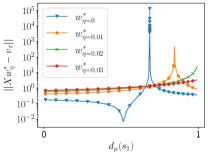
(a)

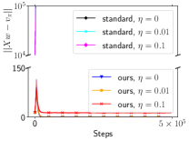
(b)

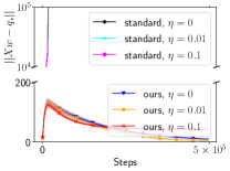
(c)

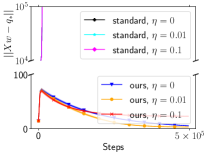
(d)

Figure 1: (a) Effect of regularization on Kolter’s example. $v_{\pi}$ is the true state-value function. (b) Policy evaluation on Baird’s example. (c) Control on Baird’s example with a fixed behavior policy. (d) Control on Baird’s example with an action-value-dependent behavior policy. In (b)(c)(d), the curves are averaged over 30 independent runs with shaded region indicating one standard deviation. $q_{*}$ is the optimal action-value function. $\eta$ is the weight for the ridge term. Those marked “ours” are curves of algorithms we propose; those marked “standard” are standard semi-gradient off-policy algorithms. Interestingly, the three “standard” curves overlap and get unbounded quickly.

Theorem 6.

Under Assumptions 2.2, 3.1, 3.5, 5.1, & 5.2, let $L_{\mu}$ denote the Lipschitz constant of $\mu_{\theta}$, for any $\xi\in(0,1),R_{B_{1}}>R_{B_{2}}>R_{B_{1}}-\xi>0$, there exist constants $C_{0}$ and $C_{1}$ such that for all $\norm{X}<C_{0},L_{\mu}<C_{1}$, the iterate $\quantity{w_{t}}$ generated by Algorithm 5 satisfies

$$\textstyle{\lim_{t\to\infty}w_{t}=w^{*}_{\eta}}\mbox{\quad almost surely,\quad}$$ (38)

where $w^{*}_{\eta}$ is the unique solution of
$(\bar{A}_{\pi_{w},\mu_{w}}+\eta I)w-\bar{b}_{\mu_{w}}={\textbf{0}}$ inside $B_{1}$, where

$$\bar{A}_{\pi_{w},\mu_{w}} \doteq X(D_{\mu_{w}}-d_{\mu_{w}}d_{\mu_{w}}^{\top})(I-P_{\pi_{w}})X,$$ (39)

$$\bar{b}_{\mu_{w}} \doteq X^{\top}(D_{\mu_{w}}-d_{\mu_{w}}d_{\mu_{w}}^{\top})r,$$ (40)

and $\pi_{w}$ is a greedy policy w.r.t. $x(s,\cdot)^{\top}w$.

We defer the proof to Section A.7. Theorem 6 requires $\mu_{\theta}$ to be sufficiently smooth, which is a standard assumption even in the on-policy setting (e.g., Melo et al. (2008); Zou et al. (2019)). It is easy to see that if (10) converges, it converges to a solution of $\bar{A}_{\pi_{w},\mu_{w}}w-\bar{b}_{\mu_{w}}={\textbf{0}}$, which we call a TD fixed point for control in the average-reward setting. Theorem 6, which shows that Algorithm 5 finds a regularized TD fixed point, is to the best of our knowledge the first theoretical study for linear $Q$-learning in the average-reward setting.

6 Experiments

All the implementations are publicly available. 

We first use Kolter’s example (Kolter, 2011) to investigate how $\eta$ influences the performance of $w^{*}_{\eta}$ in the policy evaluation setting. Details are provided in Section D.1. This example is a two-state MDP with small representation error (i.e., $\norm{\Pi_{D_{\mu}}v_{\pi}-v_{\pi}}$ is small). We vary the sampling probability of one state ($d_{\mu}(s_{1})$) and compute corresponding $w^{*}_{\eta}$ analytically. Figure 1a shows that with $\eta=0$, the performance of $w^{*}_{\eta}$ becomes arbitrarily poor when $d_{\mu}(s_{1})$ approaches around 0.71. With $\eta=0.01$, the spike exists as well. If we further increase $\eta$ to $0.02$ and $0.03$, the performance for $w^{*}_{\eta}$ becomes well bounded. This confirms the potential advantage of the regularized TD fixed points.

We then use Baird’s example (Baird, 1995) to empirically investigate the convergence of the algorithms we propose. We use exactly the same setup as Chapter 11.2 of Sutton & Barto (2018). Details are provided in Section D.2. In particular, we consider three settings: policy evaluation (Figure 1b), control with a fixed behavior policy (Figure 1c), and control with an action-value dependent behavior policy (Figure 1d). For the policy evaluation setting, we compare a TD version of Algorithm 1 and standard Off-Policy Linear TD (possibly with ridge regularization). For the two control settings, we compare Algorithm 3 with standard linear $Q$-learning (possibly with ridge regularization). We use constant learning rates and do not use any projection in all the compared algorithms. The exact update rules are provided in Section D.2. Interestingly, Figures 1b-d show that even with $\eta=0$, i.e., no ridge regularization, our algorithms with target network still converge in the tested domains. By contrast, without a target network, even when mild regularization is imposed, standard off-policy algorithms still diverge. This confirms the importance of the target network.

7 Discussion and Related Work

For all the algorithms we propose, both the target network and the ridge regularization are at play. One may wonder if it is possible to ensure convergence with only ridge regularization without the target network. In the policy evaluation setting, the answer is affirmative. Applying ridge regularization in (4) directly yields

$$w_{t+1}\leftarrow w_{t}+\alpha_{t}\delta_{t}x_{t}-\alpha_{t}\eta w_{t},$$ (41)

where $\delta_{t}$ is defined in (4). The expected update of (41) is

$$\Delta_{w} \doteq b-(A+\eta I)w$$ (42)

$$\doteq b-X^{\top}D_{\mu}Xw+\gamma X^{\top}D_{\mu}(P_{\pi}Xw)-\eta w.$$ (43)

If its Jacobian w.r.t. $w$, denoted as $J_{w}(\Delta_{w})$, is negative definite, the convergence of $\quantity{w_{t}}$ is expected (see, e.g., Section 5.5 of Vidyasagar (2002)). This negative definiteness can be easily achieved by ensuring $\eta>\norm{X}^{2}\norm{D_{\mu}(I-\gamma P_{\pi})}$ (see Diddigi et al. (2019) for similar techniques). This direct ridge regularization, however, would not work in the control setting. Consider, for example, linear $Q$-learning with ridge regularization (i.e., (41) with $\delta_{t}$ defined in (8)). The Jacobian of its expected update is $J_{w}(b_{\mu_{w}}-(A_{\pi_{w},\mu_{w}}+\eta I)w)$. It is, however, not clear how to ensure this Jacobian is negative definite by tuning $\eta$. By using a target network for bootstrapping, $P_{\pi}Xw$ becomes $P_{\pi}X\theta$. So $J_{w}(\Delta_{w})$ becomes $-J_{w}(X^{\top}D_{\mu}Xw+\eta w)$, which is always negative definite. Similarly, $J_{w}(b_{\mu_{w}}-(A_{\pi_{w},\mu_{w}}+\eta)w)$ becomes $-J_{w}(X^{\top}D_{\mu_{\theta}}Xw+\eta w)$ in Algorithm 3, which is always negative definite regardless of $\theta$. The convergence of the main network $\quantity{w_{t}}$ can, therefore, be expected. The convergence of the target network $\quantity{\theta_{t}}$ is then delegated to Theorem 1. Now it is clear that in the deadly triad setting, the target network stabilizes training by ensuring the Jacobian of the expected update is negative definite. One may also wonder if it is possible to ensure convergence with only the target network without ridge regularization. The answer is unclear. In our analysis, the conditions on $\norm{X}$ (or equivalently, $\eta$) are only sufficient and not necessarily necessary. We do see in Figure 1 that even with $\eta=0$, our algorithms still converge in the tested domains. How small $\eta$ can be in general and under what circumstances $\eta$ can be 0 are still open problems, which we leave for future work. Further, ridge regularization usually affects the convergence rate of the algorithm, which we also leave for future work.

In this paper, we investigate target network as one possible solution for the deadly triad. Other solutions include Gradient TD methods (Sutton et al. (2009b, a, 2016) for the discounted setting; Zhang et al. (2021) for the average-reward setting) and Emphatic TD methods (Sutton et al. (2016) for the discounted setting). Other convergence results of $Q$-learning with function approximation include Tsitsiklis & Van Roy (1996); Szepesvári & Smart (2004), which require special approximation architectures, Wen & Van Roy (2013); Du et al. (2020), which consider deterministic MDPs, Li et al. (2011); Du et al. (2019), which require a special oracle to guide exploration, Chen et al. (2019a), which require matrix inversion every time step, and Wang et al. (2019); Yang & Wang (2019, 2020); Jin et al. (2020), which consider linear MDPs (i.e., both $p$ and $r$ are assumed to be linear). Achiam et al. (2019) characterize the divergence of $Q$-learning with nonlinear function approximation via Taylor expansions and use preconditioning to empirically stabilize training. Van Hasselt et al. (2018) empirically study the role of a target network in the deadly triad setting in deep RL, which is complementary to our theoretical analysis.

Regularization is also widely used in RL. Yu (2017) introduce a general regularization term to improve the robustness of Gradient TD algorithms. Du et al. (2017) use ridge regularization in MSPBE to improve its convexity. Zhang et al. (2020) use ridge regularization to stabilize the training of critic in an off-policy actor-critic algorithm. Kolter & Ng (2009); Johns et al. (2010); Petrik et al. (2010); Painter-Wakefield et al. (2012); Liu et al. (2012) use Lasso regularization in policy evaluation, mainly for feature selection.

8 Conclusion

In this paper, we proposed and analyzed a novel target network update rule, with which we improved several linear RL algorithms that are known to diverge previously due to the deadly triad. Our analysis provided a theoretical understanding, in the deadly triad setting, of the conventional wisdom that a target network stabilizes training. A possibility for future work is to introduce nonlinear function approximation, possibly over-parameterized neural networks, into our analysis.

Appendix A Convergence of Target Networks

We first state a result from Borkar (2009) regarding the convergence of a linear system. Consider updating the parameter $y\in\mathbb{R}^{K}$ recursively as

$$y_{t+1}\doteq y_{t}+\beta_{t}(h(y_{t})+\epsilon_{t}),$$ (44)

where $h:\mathbb{R}^{K}\to\mathbb{R}^{K}$ and $\quantity{\epsilon_{t}}$ is a deterministic or random bounded sequence satisfying $\lim_{t\to\infty}\norm{\epsilon_{t}}=0$. Assuming

Assumption A.1.

$h$ is Lipschitz continuous.

Assumption A.2.

The learning rates $\quantity{\beta_{t}}$ satisfies $\sum_{t}\beta_{t}=\infty,\sum_{t}\beta_{t}^{2}<\infty$.

Assumption A.3.

$\sup_{t}\norm{y_{t}}<\infty$ almost surely.

Theorem 7.

(The third extension of Theorem 2 in Chapter 2 of Borkar (2009)) Under Assumptions A.1- A.3, almost surely, the sequence $\quantity{y_{t}}$ generated by (44) converges to a compact connected internally chain transitive invariant set of the ODE

$$\derivative{t}y(t)=h(y(t)).$$ (45)

A.1 Proof of Theorem 1

Proof.

Similar to Chapter 5.4 of Borkar (2009), we consider $\dot{\Gamma}_{B_{1}}$, the directional derivative of $\Gamma_{B_{1}}$. At a point $x\in\mathbb{R}^{K}$, given a direction $y\in R^{K}$, we have

$$\dot{\Gamma}_{B_{1}}(x,y) \doteq\lim_{\delta\to 0}\frac{\Gamma_{B_{1}}(x+\delta y)-\Gamma_{B_{1}}(x)}{\delta}$$ (46)

$$=\begin{cases}y,&x\in int(B_{1})\\ y,&x\in\partial B_{1},y\in F_{x}(B_{1})\\ -\frac{xx^{\top}y}{\norm{x}^{3}}+\frac{y}{\norm{x}},&\text{otherwise}\end{cases}$$ (47)

where $int(B_{1})$ is the interior of $B_{1}$, $\partial B_{1}$ is the boundary of $B_{1}$, $F_{x}(B_{1})\doteq\quantity{y\in\mathbb{R}^{K}\mid\exists\delta>0,\mbox{\quad s.t.\quad}x+\delta y\in B_{1}}$ is the feasible directions of $B_{1}$ w.r.t. $x$. The first two cases are trivial and are easy to deal with. The third case is complicated and is the source of the reflection term $\zeta(t)$ in (17). However, thanks to the projection $\Gamma_{B_{2}}$, we succeeded in getting rid of it.

By (14), $\theta_{t}\in B_{1}$ always holds. With the directional derivative, we can rewrite the update rule of $\quantity{\theta_{t}}$ as

$$\theta_{t+1} =\Gamma_{B_{1}}\big{(}\theta_{t}+\beta_{t}(\Gamma_{B_{2}}(w_{t})-\theta_{t})\big{)}$$ (48)

$$=\theta_{t}+\beta_{t}\frac{\Gamma_{B_{1}}\big{(}\theta_{t}+\beta_{t}(\Gamma_{B_{2}}(w_{t})-\theta_{t})\big{)}-\Gamma_{B_{1}}(\theta_{t})}{\beta_{t}}$$ (49)

$$=\theta_{t}+\beta_{t}\big{(}\dot{\Gamma}_{B_{1}}(\theta_{t},\Gamma_{B_{2}}(w_{t})-\theta_{t})+o(\beta_{t})\big{)}\mbox{\quad(Definition of limit)\quad}.$$ (50)

We now compute $\dot{\Gamma}_{B_{1}}(\theta_{t},\Gamma_{B_{2}}(w_{t})-\theta_{t})$. We proceed by showing that only the first two cases in $\dot{\Gamma}_{B_{1}}(x,y)$ can happen and the third case will never occur.

For $\theta_{t}\in\text{int}(B_{1})$, we have

$$\dot{\Gamma}_{B_{1}}(\theta_{t},\Gamma_{B_{2}}(w_{t})-\theta_{t})=\Gamma_{B_{2}}(w_{t})-\theta_{t}.$$ (51)

For $\theta_{t}\in\partial B_{1}$,

$$\langle{\theta_{t}},{\Gamma_{B_{2}}(w_{t})-\theta_{t}}\rangle =\langle{\theta_{t}},{\Gamma_{B_{2}}(w_{t})}\rangle-R_{B_{1}}^{2}\leq R_{B_{1}}R_{B_{2}}-R_{B_{1}}^{2}<0.$$ (52)

Let $y_{0}\doteq\Gamma_{B_{2}}(w_{t})-\theta_{t}$, (52) implies that we can decompose $y_{0}$ as $y_{0}=y_{1}+y_{2}$, where $\langle{\theta_{t}},{y_{1}}\rangle=0$ and $\langle{\theta_{t}},{y_{2}}\rangle=-\norm{\theta_{t}}\norm{y_{2}}$. Here $y_{2}$ is the projection of $y_{0}$ onto $\theta_{t}$, which is in the opposite direction of $\theta_{t}$ and $y_{1}$ is the remaining orthogonal component. By Pythagoras’s theorem, for any $\delta>0$,

$$\norm{\theta_{t}+\delta y_{0}}^{2} =\norm{\delta y_{1}}^{2}+\norm{\theta_{t}+\delta y_{2}}^{2}$$ (53)

$$=\delta^{2}\norm{y_{1}}^{2}+\norm{\theta_{t}}^{2}-2\delta\norm{\theta_{t}}\norm{y_{2}}+\delta^{2}\norm{y_{2}}^{2}.$$ (54)

For sufficiently small $\delta$, e.g., $\delta^{2}\norm{y_{1}}^{2}-2\delta\norm{\theta_{t}}\norm{y_{2}}+\delta^{2}\norm{y_{2}}^{2}<0$, we have

$$\norm{\theta_{t}+\delta y_{0}}^{2}<\norm{\theta_{t}}^{2}=R_{B_{1}}^{2},$$ (55)

implying $\Gamma_{B_{2}}(w_{t})-\theta_{t}\in F_{\theta_{t}}(B_{1})$. So we have

$$\dot{\Gamma}_{B_{1}}(\theta_{t},\Gamma_{B_{2}}(w_{t})-\theta_{t})=\Gamma_{B_{2}}(w_{t})-\theta_{t}.$$ (56)

Combining (51) and (56) yields

$$\theta_{t+1} =\theta_{t}+\beta_{t}\big{(}\Gamma_{B_{2}}(w_{t})-\theta_{t}+o(\beta_{t})\big{)}$$ (57)

$$=\theta_{t}+\beta_{t}\big{(}\Gamma_{B_{2}}(w^{*}(\theta_{t}))-\theta_{t}+o(1)+o(\beta_{t})\big{)}\mbox{\quad(Assumption~{}\ref{assu target net main net} and the continuity of $\Gamma_{B_{2}}$)\quad}$$ (58)

$$=\theta_{t}+\beta_{t}\big{(}w^{*}(\theta_{t})-\theta_{t}+o(1)+o(\beta_{t}))\mbox{\quad(Assumption~{}\ref{assu target net boundedness})\quad}$$ (59)

Assumption A.1 is verified by Assumption 3.4; Assumption A.2 is verified by Assumption 3.1; Assumption A.3 is verified directly by the projection in (14). By Theorem 7, almost surely, $\quantity{\theta_{t}}$ converges to a compact connected internally chain transitive invariant set of the ODE

$$\derivative{t}\theta(t)=w^{*}(\theta(t))-\theta(t).$$ (60)

Under Assumption 3.4, the Banach fixed-point theorem asserts that there is a unique $\theta^{*}$ satisfying $w^{*}(\theta^{*})=\theta^{*}$, i.e., $\theta^{*}$ is the unique equilibrium of the ODE above. We now show $\theta^{*}$ is globally asymptotically stable. Consider the candidate Lyapunov function

$$V(\theta)\doteq\frac{1}{2}\norm{\theta-\theta^{*}}^{2}.$$ (61)

We have

$$\derivative{t}V(\theta(t))= \langle{\theta(t)-\theta^{*}},{\derivative{t}\theta(t)}\rangle$$ (62)

$$= \langle{\theta(t)-\theta^{*}},{w^{*}(\theta(t))-\theta(t)}\rangle$$ (63)

$$= \langle{\theta(t)-\theta^{*}},{w^{*}(\theta(t))-\theta(t)-w^{*}(\theta^{*})+\theta^{*}}\rangle$$ (64)

$$\leq \varrho\norm{\theta(t)-\theta^{*}}^{2}-\norm{\theta(t)-\theta^{*}}^{2},$$ (65)

where $\varrho<1$ is the Lipschitz constant of $w^{*}$. It is easy to see

• $V(\theta)\geq 0$

• $V(\theta)=0\iff\theta=\theta^{*}$

• $\derivative{t}V(\theta(t))\leq 0$

• $\derivative{t}V(\theta(t))=0\iff\theta=\theta^{*}$

Consequently, $\theta^{*}$ is globally asymptotically stable, implying

$$\lim_{t\to\infty}\theta_{t} =\theta^{*},$$ (66)

$$\lim_{t\to\infty}w_{t} =\lim_{t\to\infty}w^{*}(\theta_{t})=w^{*}(\theta^{*})=\theta^{*}.$$ (67)

∎

A.2 Proof of Lemma 1

Proof.

By (14), $\theta_{t}\in B_{1}$ holds for all $t$. So

$$\norm{\theta_{t+1}-\theta_{t}}$$ (68)

$$= \norm{\Gamma_{B_{1}}\Big{(}\theta_{t}+\beta_{t}(\Gamma_{B_{2}}(w_{t})-\theta_{t})\Big{)}-\Gamma_{B_{1}}(\theta_{t})}$$ (69)

$$\leq \beta_{t}\norm{\Gamma_{B_{2}}(w_{t})-\theta_{t}}\mbox{\quad(Nonexpansiveness of projection)\quad}$$ (70)

$$\leq \beta_{t}(R_{B_{1}}+R_{B_{2}}).$$ (71)

∎

A.3 Proof of Theorem 2

Proof.

Consider the Markov process $Y_{t}\doteq(S_{t},A_{t},S_{t+1})$. By Assumption 4.1, $Y_{t}$ adopts a unique stationary distribution, which we refer to as $d_{\mathcal{Y}}$. We have $d_{\mathcal{Y}}(s,a,s^{\prime})=d_{\mu}(s)\mu(a|s)p(s^{\prime}|s,a)$. We define

$$h_{\theta}(s,a,s^{\prime}) \doteq\big{(}r(s,a)+\gamma\sum_{a^{\prime}}\pi(a^{\prime}|s^{\prime})x(s^{\prime},a^{\prime})^{\top}\Gamma_{B_{1}}(\theta)\big{)}x(s,a),$$ (72)

$$G_{\theta}(s,a,s^{\prime}) \doteq x(s,a)x(s,a)^{\top}+\eta I.$$ (73)

As $\theta_{t}\in B_{1}$ holds for all $t$, we can rewrite the update of $w_{t}$ in Algorithm 1 as

$$w_{t+1}=w_{t}+\alpha_{t}(h_{\theta_{t}}(Y_{t})-G_{\theta_{t}}(Y_{t})w_{t}).$$ (74)

The asymptotic behavior of $\quantity{w_{t}}$ is then governed by

$$\bar{h}(\theta) \doteq\mathbb{E}_{(s,a,s^{\prime})\sim d_{\mathcal{Y}}}[h_{\theta}(s,a,s^{\prime})]$$ (75)

$$=X^{\top}D_{\mu}r+\gamma X^{\top}D_{\mu}P_{\pi}X\Gamma_{B_{1}}(\theta),$$ (76)

$$\bar{G}(\theta) \doteq\mathbb{E}_{(s,a,s^{\prime})\sim d_{\mathcal{Y}}}[G_{\theta}(s,a,s^{\prime})]$$ (77)

$$=X^{\top}D_{\mu}X+\eta I.$$ (78)

Define

$$w^{*}(\theta)\doteq\bar{G}(\theta)^{-1}\bar{h}(\theta)=(X^{\top}D_{\mu}X+\eta I)^{-1}X^{\top}D_{\mu}(r+\gamma P_{\pi}X\Gamma_{B_{1}}(\theta)).$$ (79)

We now verify Assumptions 3.2, 3.3, & 3.4 to invoke Theorem 1.

Assumption 3.2 is verified in Lemma 2.

To verify Assumption 3.4, we use SVD and get

$$D_{\mu}^{\frac{1}{2}}X=U^{\top}\Sigma V,$$ (80)

where $U,V$ are two orthogonal matrices, $\Sigma=\matrixquantity[\Sigma_{+}\\ 0]$ is a rectangular diagonal matrix with $\Sigma_{+}\doteq diag([\dots,\sigma_{i},\dots])$ being a diagonal matrix. Assumptions 4.1 & 2.2 imply that $\sigma_{i}>0$. We have

$$\norm{(X^{\top}D_{\mu}X+\eta I)^{-1}X^{\top}D_{\mu}^{\frac{1}{2}}}= \norm{V^{\top}(\Sigma^{\top}\Sigma+\eta I)^{-1}\Sigma^{\top}U}=\norm{(\Sigma^{\top}\Sigma+\eta I)^{-1}\Sigma^{\top}}$$ (81)

$$= \norm{diag([\cdots,\frac{\sigma_{i}}{\sigma_{i}^{2}+\eta},\cdots])}=\norm{diag([\cdots,\frac{1}{\sigma_{i}+\eta/\sigma_{i}},\cdots])}=\max_{i}\frac{1}{\sigma_{i}+\eta/\sigma_{i}}$$ (82)

$$\leq \frac{1}{2\sqrt{\eta}}$$ (83)

According to (79), it is then easy to see

$$\norm{w^{*}(\theta_{1})-w^{*}(\theta_{2})} \leq\frac{\gamma}{2\sqrt{\eta}}\norm{D_{\mu}^{\frac{1}{2}}P_{\pi}}\norm{X}\norm{\Gamma_{B_{1}}(\theta_{1})-\Gamma_{B_{1}}(\theta_{2})}$$ (84)

$$\leq\frac{\gamma}{2\sqrt{\eta}}\norm{D_{\mu}^{\frac{1}{2}}P_{\pi}}\norm{X}\norm{\theta_{1}-\theta_{2}}$$ (85)

$$\leq\frac{\gamma}{2\sqrt{\eta}}\norm{D_{\mu}^{\frac{1}{2}}P_{\pi}D_{\mu}^{-\frac{1}{2}}}\norm{D_{\mu}^{\frac{1}{2}}}\norm{X}\norm{\theta_{1}-\theta_{2}}$$ (86)

$$=\frac{\gamma}{2\sqrt{\eta}}\norm{P_{\pi}}_{D_{\mu}}\norm{D_{\mu}^{\frac{1}{2}}}\norm{X}\norm{\theta_{1}-\theta_{2}}\mbox{\quad(See (20) in \cite[citet]{\@@bibref{Authors Phrase1YearPhrase2}{kolter2011fixed}{\@@citephrase{(}}{\@@citephrase{)}}})\quad}$$ (87)

$$\leq\frac{\gamma}{2\sqrt{\eta}}\norm{P_{\pi}}_{D_{\mu}}\norm{X}\norm{\theta_{1}-\theta_{2}}.$$ (88)

Take any $\xi\in(0,1)$, assuming

$$\norm{X}\leq\frac{2(1-\xi)\sqrt{\eta}}{\gamma\norm{P_{\pi}}_{D_{\mu}}},$$ (90)

then

$$\norm{w^{*}(\theta_{1})-w^{*}(\theta_{2})}\leq(1-\xi)\norm{\theta_{1}-\theta_{2}}.$$ (91)

Assumption 3.4, therefore, holds.

We now select proper $R_{B_{1}}$ and $R_{B_{2}}$ to fulfill Assumption 3.3. Plugging (81) and (90) into (79) yields

$$\norm{w^{*}(\theta)} \leq\frac{1}{2\sqrt{\eta}}\norm{D_{\mu}^{\frac{1}{2}}r}+(1-\xi)R_{B_{1}}$$ (92)

$$=R_{B_{1}}-\xi+(\frac{1}{2\sqrt{\eta}}\norm{D_{\mu}^{\frac{1}{2}}r}+\xi-\xi R_{B_{1}})$$ (93)

For sufficiently large $R_{B_{1}}$, e.g.,

$$R_{B_{1}}\geq\frac{1}{2\xi\sqrt{\eta}}\norm{D_{\mu}^{\frac{1}{2}}r}+1,$$ (94)

we have $\sup_{\theta}\norm{w^{*}(\theta)}\leq R_{B_{1}}-\xi$. Selecting $R_{B_{2}}\in(R_{B_{1}}-\xi,R_{B_{1}})$ then fulfills Assumption 3.3.

With Assumptions 3.1 - 3.4 satisfied, Theorem 1 then implies that there exists a unique $\theta_{\infty}$ such that

$$w^{*}(\theta_{\infty})=\theta_{\infty}\mbox{\quad and\quad}\lim_{t\to\infty}\theta_{t}=\lim_{t\to\infty}w_{t}=\theta_{\infty}.$$ (95)

Next we show what $\theta_{\infty}$ is. We define

$$f(\theta)\doteq(X^{\top}D_{\mu}X+\eta I)^{-1}X^{\top}D_{\mu}(r+\gamma P_{\pi}X\theta).$$ (96)

Note this is just the right side of equation (79) without the projection. (81) and (90) imply that $f$ is a contraction. The Banach fixed-point theorem then asserts that $f$ adopts a unique fixed point, which we refer to as $w^{*}_{\eta}$. We have

$$\norm{w^{*}_{\eta}} =\norm{f(w^{*}_{\eta})}\leq\frac{1}{2\sqrt{\eta}}(\norm{r}+\gamma\norm{P_{\pi}}_{D_{\mu}}\norm{X}\norm{w^{*}_{\eta}})$$ (97)

$$\leq\frac{\norm{r}}{2\sqrt{\eta}}+(1-\xi)\norm{w^{*}_{\eta}}\mbox{\quad(By~{}\eqref{eq:op-td-inequ1})\quad}$$ (98)

$$\implies\norm{w^{*}_{\eta}} \leq\frac{\norm{r}}{2\xi\sqrt{\eta}}$$ (99)

Then for sufficiently large $R_{B_{1}}$, e.g.,

$$R_{B_{1}}\geq\frac{\norm{r}}{2\xi\sqrt{\eta}},$$ (100)

we have $w^{*}_{\eta}=\Gamma_{B_{1}}(w^{*}_{\eta})$, implying $w^{*}_{\eta}$ is a fixed point of $w^{*}(\cdot)$ (i.e., the right side of (79)) as well. As $w^{*}(\cdot)$ is a contraction, we have $\theta_{\infty}=w^{*}_{\eta}$. Rewriting $f(w^{*}_{\eta})=w^{*}_{\eta}$ yields

$$Aw^{*}_{\eta}+\eta w^{*}_{\eta}-b ={\textbf{0}}.$$ (101)

In other words, $w^{*}_{\eta}$ is the unique (due to the contraction of $f$) solution of $(A+\eta I)w-b={\textbf{0}}$.

Combining (90),  (94), and (100), the desired constants are

$$C_{0} \doteq\frac{2(1-\xi)\sqrt{\eta}}{\gamma\norm{P_{\pi}}_{D_{\mu}}},$$ (102)

$$C_{1} \doteq\frac{\norm{r}}{2\xi\sqrt{\eta}}+1.$$ (103)

We now bound $\norm{Xw^{*}_{\eta}-q_{\pi}}$. For any $y\in\mathbb{R}^{|\mathcal{S}|}$, we define the ridge regularized projection $\Pi^{\eta}_{D_{\mu}}$ as

$$\Pi^{\eta}_{D_{\mu}}y \doteq X\arg\min_{w}\left(\norm{Xw-y}^{2}_{D_{\mu}}+\eta\norm{w}^{2}\right)$$ (104)

$$=X(X^{\top}D_{\mu}X+\eta I)^{-1}X^{\top}D_{\mu}y.$$ (105)

$\Pi_{D_{\mu}}^{\eta}$ is connected with $f$ as $\Pi_{D_{\mu}}^{\eta}{\mathcal{T}}_{\pi}(Xw)=Xf(w)$. We have

$$\norm{Xw^{*}_{\eta}-q_{\pi}} \leq\norm{Xw^{*}_{\eta}-\Pi^{\eta}_{D_{\mu}}q_{\pi}}+\norm{\Pi^{\eta}_{D_{\mu}}q_{\pi}-q_{\pi}}$$ (106)

$$=\norm{Xf(w^{*}_{\eta})-\Pi^{\eta}_{D_{\mu}}q_{\pi}}+\norm{\Pi^{\eta}_{D_{\mu}}q_{\pi}-q_{\pi}}$$ (107)

$$=\norm{\Pi^{\eta}_{D_{\mu}}{\mathcal{T}}_{\pi}(Xw^{*}_{\eta})-\Pi^{\eta}_{D_{\mu}}{\mathcal{T}}_{\pi}q_{\pi}}+\norm{\Pi^{\eta}_{D_{\mu}}q_{\pi}-q_{\pi}}$$ (108)

$$=\norm{\Pi^{\eta}_{D_{\mu}}\gamma P_{\pi}Xw^{*}_{\eta}-\Pi^{\eta}_{D_{\mu}}\gamma P_{\pi}q_{\pi}}+\norm{\Pi^{\eta}_{D_{\mu}}q_{\pi}-q_{\pi}}$$ (109)

$$=\norm{\gamma\Pi^{\eta}_{D_{\mu}}P_{\pi}(Xw^{*}_{\eta}-q_{\pi})}+\norm{\Pi^{\eta}_{D_{\mu}}q_{\pi}-q_{\pi}}$$ (110)

$$\leq\norm{\gamma X(X^{\top}D_{\mu}X+\eta I)^{-1}X^{\top}D_{\mu}P_{\pi}}\norm{Xw^{*}_{\eta}-q_{\pi}}+\norm{\Pi^{\eta}_{D_{\mu}}q_{\pi}-q_{\pi}}$$ (111)

$$\leq(1-\xi)\norm{Xw^{*}_{\eta}-q_{\pi}}+\norm{\Pi^{\eta}_{D_{\mu}}q_{\pi}-q_{\pi}}\mbox{\quad(By \eqref{eq:op-td-contraction} and \eqref{eq:op-td-inequ1})\quad}$$ (112)

The above equation implies

$$\norm{Xw^{*}_{\eta}-q_{\pi}} \leq\frac{1}{\xi}\norm{\Pi^{\eta}_{D_{\mu}}q_{\pi}-q_{\pi}}\leq\frac{1}{\xi}\left(\norm{\Pi^{\eta}_{D_{\mu}}q_{\pi}-\Pi_{D_{\mu}}q_{\pi}}+\norm{\Pi_{D_{\mu}}q_{\pi}-q_{\pi}}\right),$$ (114)

where $\Pi_{D_{\mu}}$ is shorthand for $\Pi_{D_{\mu}}^{\eta=0}$. We now bound $\norm{\Pi^{\eta}_{D_{\mu}}-\Pi_{D_{\mu}}}$.

$$\norm{\Pi^{\eta}_{D_{\mu}}-\Pi_{D_{\mu}}} \leq\norm{X}\norm{(X^{\top}D_{\mu}X+\eta I)^{-1}-(X^{\top}D_{\mu}X)^{-1}}\norm{X^{\top}D_{\mu}}$$ (115)

$$=\norm{D_{\mu}^{-\frac{1}{2}}D_{\mu}^{\frac{1}{2}}X}\norm{V^{\top}\big{(}(\Sigma_{+}^{2}+\eta I)^{-1}-\Sigma_{+}^{-2}\big{)}V}\norm{X^{\top}D_{\mu}^{\frac{1}{2}}D_{\mu}^{\frac{1}{2}}}$$ (116)

$$\leq\norm{D_{\mu}^{-\frac{1}{2}}}\norm{\Sigma}\norm{(\Sigma_{+}^{2}+\eta I)^{-1}-\Sigma_{+}^{-2}}\norm{\Sigma}\norm{D_{\mu}^{\frac{1}{2}}}$$ (117)

$$\leq\norm{D_{\mu}^{-\frac{1}{2}}}\norm{\Sigma}\norm{diag([\dots,\frac{\eta}{\sigma_{i}^{2}(\eta+\sigma_{i}^{2})},\dots])}\norm{\Sigma}\norm{D_{\mu}^{\frac{1}{2}}}$$ (118)

$$\leq\norm{D_{\mu}^{-\frac{1}{2}}}\norm{\Sigma}\max_{i}\frac{\eta}{\sigma_{i}^{2}(\eta+\sigma_{i}^{2})}\norm{\Sigma}\norm{D_{\mu}^{\frac{1}{2}}}$$ (119)

$$\leq\norm{D_{\mu}^{-\frac{1}{2}}}\norm{\Sigma}^{2}\max_{i}\frac{\eta}{\sigma_{i}^{4}}\norm{D_{\mu}^{\frac{1}{2}}}$$ (120)

$$\leq\norm{D_{\mu}^{-\frac{1}{2}}}\frac{\sigma_{\max}(\Sigma)^{2}}{\sigma_{\min}(\Sigma)^{4}}\norm{D_{\mu}^{\frac{1}{2}}}\eta$$ (121)

($$\sigma_{\max}(\cdot) \sigma_{\min}(\cdot)$$ and indicate the largest and smallest singular values)

$$=\frac{\sigma_{\max}(D_{\mu}^{\frac{1}{2}}X)^{2}}{\sigma_{\min}(D_{\mu}^{\frac{1}{2}}X)^{4}}\frac{\sigma_{\max}(D_{\mu}^{\frac{1}{2}})}{\sigma_{\min}(D_{\mu}^{\frac{1}{2}})}\eta$$ (122)

$$\leq\frac{\sigma_{\max}(X)^{2}}{\sigma_{\min}(X)^{4}\sigma_{\min}(D_{\mu})^{2.5}}\eta$$ (123)

($$\sigma_{\max}(XY)\leq\sigma_{\max}(X)\sigma_{\max}(Y);\sigma_{\min}(XY)\geq\sigma_{\min}(X)\sigma_{\min}(Y)$$ )

. (124)

Finally, we arrive at

$$\norm{Xw^{*}_{\eta}-q_{\pi}} \leq\frac{1}{\xi}\Big{(}\frac{\sigma_{\max}(X)^{2}}{\sigma_{\min}(X)^{4}\sigma_{\min}(D_{\mu})^{2.5}}\norm{q_{\pi}}\eta+\norm{\Pi_{D_{\mu}}q_{\pi}-q_{\pi}}\Big{)},$$ (125)

which completes the proof. ∎

A.4 Proof of Theorem 3

Proof.

The proof is similar to the proof of Theorem 2 in Section A.3. We, therefore, highlight only the difference to avoid verbatim repetition. Define

(126)

We can then rewrite the update of $\bar{r}$ and $w$ in Algorithm 2 as

$$u_{t+1}=u_{t}+\alpha_{t}(h_{\theta_{t}}(Y_{t})-G_{\theta_{t}}(Y_{t})u_{t}).$$ (127)

Similarly, we define

(128)

(129)

We proceed to verifying Assumptions 3.2, 3.3, & 3.4 to invoke Theorem 1.

Assumption 3.2 is verified in Lemma 3.

For Assumption 3.4 to hold, note

$$\norm{\bar{G}(\theta)^{-1}} =\max\quantity{1,\norm{(X^{\top}D_{\mu}X+\eta I)^{-1}}}\leq\max\quantity{1,\frac{1}{\eta}}$$ (130)

$$\norm{\bar{H}_{2}}^{2} =\max_{\norm{u}=1}\norm{\bar{H}_{2}u}^{2}=\max_{\norm{u}=1}\norm{\matrixquantity[d_{\mu}^{\top}(P_{\pi}-I)Xw\\ -X^{\top}d_{\mu}\bar{r}+X^{\top}D_{\mu}P_{\pi}Xw]}^{2}$$ (131)

$$=\max_{\norm{u}=1}\norm{d_{\mu}^{\top}(P_{\pi}-I)Xw}^{2}+\norm{-X^{\top}d_{\mu}\bar{r}+X^{\top}D_{\mu}P_{\pi}Xw}^{2}$$ (132)

$$\leq\max_{\norm{u}=1}\norm{d_{\mu}^{\top}(P_{\pi}-I)X}^{2}\norm{w}^{2}+2\norm{X^{\top}d_{\mu}}^{2}\norm{\bar{r}}^{2}+2\norm{X^{\top}D_{\mu}P_{\pi}X}^{2}\norm{w}^{2}$$ (133)

$$\leq\max\quantity{\norm{d_{\mu}^{\top}(P_{\pi}-I)X}^{2}+2\norm{X^{\top}D_{\mu}P_{\pi}X}^{2},2\norm{X^{\top}d_{\mu}}^{2}}$$ (134)

$$\implies\norm{\bar{H}_{2}} \leq\norm{X}\max\quantity{\norm{d_{\mu}^{\top}(P_{\pi}-I)}+\sqrt{2}\norm{D_{\mu}P_{\pi}},\sqrt{2}\norm{d_{\mu}}}.$$ (135)

The above equations suggest that

$$\norm{u^{*}(\theta_{1})-u^{*}(\theta_{2})} \leq\max\quantity{1,\frac{1}{\eta}}\norm{X}\max\quantity{\norm{d_{\mu}^{\top}(P_{\pi}-I)}+\sqrt{2}\norm{D_{\mu}P_{\pi}},\sqrt{2}\norm{d_{\mu}}}\norm{\theta_{1}-\theta_{2}}.$$ (136)

Take any $\xi\in(0,1)$, assuming

$$\norm{X}\leq\frac{1-\xi}{\max\quantity{1,\frac{1}{\eta}}\max\quantity{\norm{d_{\mu}^{\top}(P_{\pi}-I)}+\sqrt{2}\norm{D_{\mu}P_{\pi}},\sqrt{2}\norm{d_{\mu}}}},$$ (137)

then

$$\norm{u^{*}(\theta_{1})-u^{*}(\theta_{2})}\leq(1-\xi)\norm{\theta_{1}-\theta_{2}}.$$ (138)

Assumption 3.4, therefore, holds.

We now select proper $R_{B_{1}}$ and $R_{B_{2}}$ to fulfill Assumption 3.3. Using (137), it is easy to see

$$\norm{u^{*}(\theta)}\leq\max\quantity{1,\frac{1}{\eta}}\norm{\bar{h}_{1}}+(1-\xi)R_{B_{1}}.$$ (139)

For sufficiently large $R_{B_{1}}$, e.g.,

$$R_{B_{1}}\geq\max\quantity{1,\frac{1}{\eta}}\frac{\norm{\bar{h}_{1}}}{\xi}+1,$$ (140)

we have $\sup_{\theta}\norm{w^{*}(\theta)}\leq R_{B_{1}}-\xi$. Selecting $R_{B_{2}}\in(R_{B_{1}}-\xi,R_{B_{1}})$ then fulfills Assumption 3.3.

With Assumptions 3.1 - 3.4 satisfied, Theorem 1 then implies that there exists a unique $\theta_{\infty}$ such that

$$u^{*}(\theta_{\infty})=\theta_{\infty}\mbox{\quad and\quad}\lim_{t\to\infty}\theta_{t}=\lim_{t\to\infty}u_{t}=\theta_{\infty}.$$ (141)

Next we show what $\theta_{\infty}$ is. We define

$$f(\theta)\doteq\bar{G}(\theta)^{-1}(\bar{h}_{1}+\bar{H}_{2}\theta).$$ (142)

Note this is just $u^{*}(\theta)$ without the projection. Under (137), it is easy to show $f$ is a contraction. The Banach fixed-point theorem then asserts that $f$ adopts a unique fixed point, which we refer to as $u^{*}_{\eta}$. Using (137) again, we get

$$\norm{u^{*}_{\eta}} =\norm{f(u^{*}_{\eta})}\leq\max\quantity{1,\frac{1}{\eta}}\norm{\bar{h}_{1}}+(1-\xi)\norm{w^{*}_{\eta}}$$ (143)

$$\implies\norm{u^{*}_{\eta}} \leq\max\quantity{1,\frac{1}{\eta}}\frac{\norm{\bar{h}_{1}}}{\xi}$$ (144)

Then for sufficiently large $R_{B_{1}}$, e.g.,

$$R_{B_{1}}\geq\max\quantity{1,\frac{1}{\eta}}\frac{\norm{\bar{h}_{1}}}{\xi},$$ (145)

we have $u^{*}_{\eta}=\Gamma_{B_{1}}(u^{*}_{\eta})$, implying $u^{*}_{\eta}$ is a fixed point of $u^{*}(\cdot)$ as well. As $u^{*}(\cdot)$ is a contraction, we have $\theta_{\infty}=u^{*}_{\eta}$. Writing $u^{*}_{\eta}$ as $\matrixquantity[\bar{r}^{*}_{\eta}\\ w^{*}_{\eta}]$ and expanding $f(u^{*}_{\eta})=u^{*}_{\eta}$ yields

$$\bar{r}^{*}_{\eta} =d_{\mu}^{\top}(r+P_{\pi}Xw^{*}_{\eta}-Xw^{*}_{\eta}),$$ (146)

$$(X^{\top}D_{\mu}X+\eta I)w^{*}_{\eta} =X^{\top}D_{\mu}r-X^{\top}d_{\mu}\bar{r}^{*}_{\eta}+X^{\top}D_{\mu}P_{\pi}Xw^{*}_{\eta}.$$ (147)

Rearranging terms yields $(\bar{A}+\eta I)w^{*}_{\eta}-\bar{b}=0$, i.e., $w^{*}_{\eta}$ is the unique (due to the contraction of $f$) solution of $(\bar{A}+\eta I)w-\bar{b}=0$.

We now bound $\norm{Xw^{*}_{\eta}-\bar{q}_{\pi}^{c}}$.

$$\norm{Xw^{*}_{\eta}-\bar{q}_{\pi}^{c}} \leq\norm{Xw^{*}_{\eta}-\Pi^{\eta}_{D_{\mu}}\bar{q}_{\pi}^{c}}+\norm{\Pi^{\eta}_{D_{\mu}}\bar{q}_{\pi}^{c}-\bar{q}_{\pi}^{c}}$$ (148)

$$=\norm{X(X^{\top}D_{\mu}X+\eta I)^{-1}(X^{\top}D_{\mu}r-X^{\top}d_{\mu}\bar{r}^{*}_{\eta}+X^{\top}D_{\mu}P_{\pi}Xw^{*}_{\eta})-\Pi^{\eta}_{D_{\mu}}\bar{q}_{\pi}^{c}}+\norm{\Pi^{\eta}_{D_{\mu}}\bar{q}_{\pi}^{c}-\bar{q}_{\pi}^{c}}$$ (149)

$$=\norm{\Pi_{D_{\mu}}^{\eta}(r+P_{\pi}Xw^{*}_{\eta})-\Pi_{D_{\mu}}^{\eta}(r+P_{\pi}\bar{q}_{\pi}^{c})}+\norm{\Pi^{\eta}_{D_{\mu}}\bar{q}_{\pi}^{c}-\bar{q}_{\pi}^{c}}\mbox{\quad(Using $X^{\top}d_{\mu}={\textbf{0}}$)\quad}$$ (150)

$$=\norm{\Pi^{\eta}_{D_{\mu}}P_{\pi}(Xw^{*}_{\eta}-\bar{q}_{\pi}^{c})}+\norm{\Pi^{\eta}_{D_{\mu}}\bar{q}_{\pi}^{c}-\bar{q}_{\pi}^{c}}$$ (151)

$$\leq\norm{X(X^{\top}D_{\mu}X+\eta I)^{-1}X^{\top}D_{\mu}P_{\pi}}\norm{Xw^{*}_{\eta}-\bar{q}_{\pi}^{c}}+\norm{\Pi^{\eta}_{D_{\mu}}\bar{q}_{\pi}^{c}-\bar{q}_{\pi}^{c}}$$ (152)

$$\leq\frac{1}{\eta}\norm{X}^{2}\norm{D_{\mu}P_{\pi}}\norm{Xw^{*}_{\eta}-\bar{q}_{\pi}^{c}}+\norm{\Pi^{\eta}_{D_{\mu}}\bar{q}_{\pi}^{c}-\bar{q}_{\pi}^{c}}.$$ (153)

Assuming

$$\norm{X}^{2}\leq\frac{(1-\xi)\eta}{\norm{D_{\mu}P_{\pi}}},$$ (154)

we have

$$\norm{Xw^{*}_{\eta}-\bar{q}_{\pi}^{c}}\leq\frac{1}{\xi}\norm{\Pi^{\eta}_{D_{\mu}}\bar{q}_{\pi}^{c}-\bar{q}_{\pi}^{c}}\leq\frac{1}{\xi}\Big{(}\frac{\sigma_{\max}(X)^{2}}{\sigma_{\min}(X)^{4}\sigma_{\min}(D_{\mu})^{2.5}}\norm{\bar{q}_{\pi}^{c}}\eta+\norm{\Pi_{D_{\mu}}\bar{q}_{\pi}^{c}-\bar{q}_{\pi}^{c}}\Big{)}\mbox{\quad(c.f.~{}\eqref{eq:regularized projection bound})\quad}.$$ (155)

It is then easy to see

$$|\bar{r}^{*}_{\eta}-\bar{r}_{\pi}|\leq\norm{d_{\mu}^{\top}(P_{\pi}-I)(Xw^{*}_{\eta}-\bar{q}_{\pi}^{c})}\leq\frac{1}{\xi}\norm{d_{\mu}^{\top}(P_{\pi}-I)}\Big{(}\frac{\sigma_{\max}(X)^{2}}{\sigma_{\min}(X)^{4}\sigma_{\min}(D_{\mu})^{2.5}}\norm{\bar{q}_{\pi}^{c}}\eta+\norm{\Pi_{D_{\mu}}\bar{q}_{\pi}^{c}-\bar{q}_{\pi}^{c}}\Big{)}.$$ (156)

Taking infimum for $c\in\mathbb{R}$ then yields the desired results.

Combining (137), (140), (145), and (154), the desired constants are

$$C_{0} \doteq\min\quantity{\frac{1-\xi}{\max\quantity{1,\frac{1}{\eta}}\max\quantity{\norm{d_{\mu}^{\top}(P_{\pi}-I)}+\sqrt{2}\norm{D_{\mu}P_{\pi}},\sqrt{2}\norm{d_{\mu}}}},\sqrt{\frac{(1-\xi)\eta}{\norm{D_{\mu}P_{\pi}}}}},$$ (157)

$$C_{1} \doteq\max\quantity{1,\frac{1}{\eta}}\frac{\norm{\bar{h}_{1}}}{\xi}+1,$$ (158)

which completes the proof. ∎

A.5 Proof of Theorem 4

Proof.

The proof is similar to the proof of Theorem 2 in Section A.3 but is more involving. We define

$$h_{\theta}(s,a,s^{\prime}) \doteq\big{(}r(s,a)+\gamma\max_{a^{\prime}}x(s^{\prime},a^{\prime})^{\top}\bar{\theta}\big{)}x(s,a),$$ (159)

$$G_{\theta}(s,a,s^{\prime}) \doteq x(s,a)x(s,a)^{\top}+\eta I,$$ (160)

where $\bar{\theta}\doteq\Gamma_{B_{1}}(\theta)$ is shorthand. As $\theta_{t}\in B_{1}$ holds for all $t$, we can rewrite the update of $w_{t}$ in Algorithm 3 as

$$w_{t+1}=w_{t}+\alpha_{t}(h_{\theta_{t}}(Y_{t})-G_{\theta_{t}}(Y_{t})w_{t}).$$ (161)

The expected update given $\theta$ is then controlled by

$$\bar{h}(\theta) \doteq\mathbb{E}_{(s,a)\sim d_{\mu_{\theta}},s^{\prime}\sim p(\cdot|s,a)}[h_{\theta}(s,a,s^{\prime})]$$ (162)

$$=X^{\top}D_{\mu_{\theta}}r+\gamma X^{\top}D_{\mu_{\theta}}P_{\pi_{\bar{\theta}}}X\bar{\theta},$$ (163)

$$\bar{G}(\theta) \doteq\mathbb{E}_{(s,a)\sim d_{\mu_{\theta}},s^{\prime}\sim p(\cdot|s,a)}[G_{\theta}(s,a,s^{\prime})]$$ (164)

$$=X^{\top}D_{\mu_{\theta}}X+\eta I,$$ (165)

where Assumption 5.1 ensures the existence of $d_{\mu_{\theta}}$ and $\pi_{\theta}$ is the target policy, i.e. a greedy policy with random tie breaking defined as follows.

Let $\mathcal{A}^{\max}_{s,\theta}\doteq\arg\max_{a}x(s,a)^{\top}\theta$ be the set of maximizing actions for state $s$, we define

$$\pi_{\theta}(a|s)\doteq\begin{cases}\frac{1}{|\mathcal{A}^{\max}_{s,\theta}|},&a\in\mathcal{A}^{\max}_{s,\theta}\\ 0,&\text{otherwise}\end{cases}.$$ (166)

Similar to the proof in Section A.3, we define

$$w^{*}(\theta)\doteq\bar{G}(\theta)^{-1}\bar{h}(\theta)=(X^{\top}D_{\mu_{\theta}}X+\eta I)^{-1}X^{\top}D_{\mu_{\theta}}(r+\gamma P_{\pi_{\bar{\theta}}}X\bar{\theta})$$ (167)

and proceed to verify Assumptions 3.2 - 3.4 to invoke Theorem 1.

Assumption 3.2 is proved in Lemma 4.

For Assumption 3.4, Lemma 10 shows that $w^{*}(\theta)$ is Lipschitz continuous in $\theta$ with

$$C_{w}\doteq\eta^{-1}\norm{X}\norm{r}L_{D}+\eta^{-2}\norm{X}^{3}\norm{r}L_{D}+\gamma\eta^{-1}L_{0}\norm{X}^{2}+\gamma U_{P}\norm{X}R_{B_{1}}(\eta^{-1}\norm{X}L_{D}+\eta^{-2}\norm{X}^{3}L_{D})$$ (168)

being a Lipschitz constant. Here $L_{D}$, $L_{0}$, and $U_{P}$ are positive constants detailed in the proof of Lemma 10. Assuming

$$\norm{X}\leq 1\mbox{\quad and\quad}\gamma U_{P}\norm{X}R_{B_{1}}\leq 1,$$ (169)

we have

$$C_{w}\leq\eta^{-2}\norm{X}(\eta\norm{r}L_{D}+\norm{r}L_{D}+\gamma\eta L_{0}+\eta L_{D}+L_{D}).$$ (170)

Take any $\xi\in(0,1)$, assuming

$$\norm{X}\leq(1-\xi)\eta^{2}(\eta\norm{r}L_{D}+\norm{r}L_{D}+\gamma\eta L_{0}+\eta L_{D}+L_{D})^{-1},$$ (171)

it then follows that $C_{w}\leq 1-\xi$. Assumptions 3.4, therefore, holds.

We now select proper $R_{B_{1}}$ and $R_{B_{2}}$ to fulfill Assumption 3.3. Similar to Lemma 10 (see, e.g., the last three rows of Table 1 in the proof of Lemma 10), we can easily get

$$\norm{w^{*}(\theta)}\leq\eta^{-1}\norm{X}\norm{r}+\gamma\eta^{-1}\norm{X}U_{P}\norm{X}R_{B_{1}}.$$ (172)

Using (169) yields

$$\norm{w^{*}(\theta)}\leq\eta^{-1}\norm{X}(\norm{r}+1).$$ (173)

For sufficiently large $R_{B_{1}}$, e.g.,

$$R_{B_{1}}>\eta^{-1}\norm{X}(\norm{r}+1)+\xi,$$ (174)

we have $\sup_{\theta}\norm{w^{*}(\theta)}<R_{B_{1}}-\xi$. Taking $R_{B_{2}}\in(R_{B_{1}}-\xi,R_{B_{1}})$ then fulfills Assumption 3.3.

With Assumptions 3.1 - 3.4 satisfied, Theorem 1 implies that there exists a unique $\theta_{\infty}$ such that

$$w^{*}(\theta_{\infty})=\theta_{\infty}\mbox{\quad and\quad}\lim_{t\to\infty}\theta_{t}=\lim_{t\to\infty}w_{t}=\theta_{\infty}.$$ (175)

We now show what $\theta_{\infty}$ is. We define

$$f(\theta)\doteq(X^{\top}D_{\mu_{\theta}}X+\eta I)^{-1}X^{\top}D_{\mu_{\theta}}(r+\gamma P_{\pi_{{\theta}}}X{\theta})$$ (176)

and consider a ball $B_{0}\doteq\quantity{\theta\in\mathbb{R}^{K}\mid\norm{\theta}\leq R_{B_{0}}}$ with $R_{B_{0}}$ to be tuned (for the Brouwer fixed-point theorem). We have

$$\norm{f(\theta)} \leq\eta^{-1}\norm{X}\norm{r}+\gamma\eta^{-1}\norm{X}^{2}U_{P}\norm{\theta}$$ (177)

Assuming

$$\gamma\eta^{-1}\norm{X}^{2}U_{P}<1-\xi,$$ (178)

we have

$$\norm{f(\theta)} \leq\eta^{-1}\norm{X}\norm{r}+(1-\xi)\norm{\theta}$$ (179)

$$=R_{B_{0}}-(R_{B_{0}}-(1-\xi)\norm{\theta}-\eta^{-1}\norm{X}\norm{r}).$$ (180)

Then for sufficiently large $R_{B_{0}}$, e.g.,

$$R_{B_{0}}\geq\frac{\norm{X}\norm{r}}{\eta\xi},$$ (181)

we have

$$\theta\in B_{0}\implies f(\theta)\in B_{0}.$$ (182)

The Brouwer fixed-point theorem then asserts that there exists a $w^{*}_{\eta}\in B_{0}$ such that $f(w^{*}_{\eta})=w^{*}_{\eta}$. For sufficiently large $R_{B_{1}}$, e.g.,

$$R_{B_{1}}>R_{B_{0}},$$ (183)

we have $\Gamma_{B_{1}}(w^{*}_{\eta})=w^{*}_{\eta}$, i.e., $w^{*}_{\eta}$ is also a fixed point of $w^{*}(\cdot)$. The contraction of $w^{*}(\cdot)$ then implies $\theta_{\infty}=w^{*}_{\eta}$. Rewriting $f(w^{*}_{\eta})=w^{*}_{\eta}$ yields

$$A_{\pi_{w^{*}_{\eta}},\mu_{w^{*}_{\eta}}}w^{*}_{\eta}+\eta w^{*}_{\eta}-b_{\mu_{w^{*}_{\eta}}} ={\textbf{0}}.$$ (184)

In other words, $w^{*}_{\eta}$ is the unique solution of $(A_{\pi_{w},\mu_{w}}+\eta I)w-b_{\mu_{w}}={\textbf{0}}$ inside $B_{1}$ (due to the contraction of $w^{*}(\cdot)$). Combining (169) (171) (178) (174) (183), the desired constant is

$$C_{0}\doteq\min\{ 1,\frac{1}{\gamma U_{P}R_{B_{1}}},\frac{\eta(R_{B_{1}}-\xi)}{\norm{r}+1},\sqrt{\frac{\eta(1-\xi)}{\gamma U_{P}}},\frac{R_{B_{1}}\eta\xi}{\norm{r}},$$ (185)

$$\frac{(1-\xi)\eta^{2}}{\eta\norm{r}L_{D}+\norm{r}L_{D}+\gamma\eta L_{0}+\eta L_{D}+L_{D}}\},$$ (186)

which completes the proof. As $R_{B_{1}}$ is usually large, in general $C_{0}$ is $\mathcal{O}(R_{B_{1}}^{-1})$. Though $C_{0}$ is potentially small, we can use small $\eta$ as well. So a small $C_{0}$ (i.e., $\norm{X}$) does not necessarily implies a large regularization bias. ∎

A.6 Proof of Theorem 5

Proof.

Let $\kappa_{t}\doteq[u_{t}^{\top},w_{t}^{\top}]^{\top}$, Algorithms 4 implies that

$$\kappa_{t+1}=\kappa_{t}+\alpha_{t}(h_{\theta_{t}}(Y_{t})-G_{\theta_{t}}(Y_{t})\kappa_{t}),$$ (187)

where

(188)

We define

(189)

(190)

(191)

where $[\cdot]_{K+1:2K}$ is the subvector indexed from $K+1$ to $2K$.

We proceed to verifying Assumptions 3.2, 3.3, & 3.4 thus invoke Theorem 1.

Assumption 3.2 is verified in Lemma 5. Lemma 11 shows that if $\norm{X}\leq 1$, there exist a constant $L_{w}>0$, which depends on $X$ through only $\frac{X}{\norm{X}}$, such that

$$\norm{w^{*}(\theta_{1})-w^{*}(\theta_{2})}\leq L_{w}\norm{X}\norm{\theta_{1}-\theta_{2}}.$$ (192)

As $w^{*}(\cdot)$ is independent of $R_{B_{1}}$, so does $L_{w}$. So as long as

$$\norm{X}\leq C_{0}\doteq\min\quantity{1,\frac{1-\xi}{L_{w}}},$$ (193)

$w^{*}(\cdot)$ is contractive and Assumption 3.4 is satisfied. Since $L_{w}$ depends on $X$ only through $\frac{X}{\norm{X}}$, there are indeed $X$ satisfying (193). E.g., if some $X^{\prime}$ does not satisfy (193), we can simply scale $X^{\prime}$ down by some scalar. In the proof of Lemma 11, we show $\sup_{\theta}\norm{C_{\mu_{\theta}}^{-1}}<\infty$. It is then easy to see $\sup_{\theta}\norm{w^{*}(\theta)}<\infty$. Consequently, we can choose sufficiently large $R_{B_{1}}$ and $R_{B_{2}}$ such that Assumption 3.3 holds.

With Assumptions 3.1 - 3.4 satisfied, Theorem 1 implies that there exists a unique $w^{*}_{\eta}$ such that

$$w^{*}(w^{*}_{\eta})=w^{*}_{\eta}\mbox{\quad and\quad}\lim_{t\to\infty}\theta_{t}=\lim_{t\to\infty}w_{t}=w^{*}_{\eta}.$$ (194)

Expanding $w^{*}(w^{*}_{\eta})=w^{*}_{\eta}$ yields

$$w^{*}_{\eta}=(A_{\pi_{w^{*}_{\eta}},\mu_{w^{*}_{\eta}}}^{\top}C_{\mu_{w^{*}_{\eta}}}^{-1}A_{\pi_{w^{*}_{\eta}},\mu_{w^{*}_{\eta}}}+\eta I)^{-1}A_{\pi_{w^{*}_{\eta}},\mu_{w^{*}_{\eta}}}^{\top}C_{\mu_{w^{*}_{\eta}}}^{-1}b_{\mu_{w^{*}_{\eta}}},$$ (195)

which completes the proof. ∎

A.7 Proof of Theorem 6

Proof.

The proof is combination of the proofs of Theorem 3 and Theorem 4. To avoid verbatim repetition, in this proof, we show only the existence of the constants $C_{0}$ and $C_{1}$ without showing the exact expressions. We define

(196)

We can then rewrite the update of $\bar{r}$ and $w$ in Algorithm 5 as

$$u_{t+1}=u_{t}+\alpha_{t}(h_{\theta_{t}}(Y_{t})-G_{\theta_{t}}(Y_{t})u_{t}).$$ (197)

In the rest of this proof, we write $\mu_{\theta}$ and $\pi_{\theta}$ as shorthand for $\mu_{\theta^{w}}$ and $\pi_{\theta^{w}}$. We define

(198)

(199)

We proceed to verifying Assumptions 3.2, 3.3, & 3.4 to invoke Theorem 1.

Assumption 3.2 is verified in Lemma 6.

For Assumption 3.4, Lemma 12 suggests that assuming $\norm{X}\leq 1$, $L_{\mu}\leq 1$, then

$$C_{u}=\max\quantity{1,\eta^{-1}}(\mathcal{O}(\norm{X})+\mathcal{O}(L_{\mu}))+\max\quantity{1,\eta^{-2}}\mathcal{O}(\norm{X})$$ (200)

is a Lipschitz constant of $u^{*}(\theta)$. Take any $\xi\in(0,1)$, it is easy to see there exists positive constants $C_{2}$ and $C_{3}$ such that

$$\norm{X}\leq C_{2},L_{\mu}\leq C_{3}\implies C_{u}\leq 1-\xi.$$ (201)

Assumption 3.4, therefore, holds.

We now select proper $R_{B_{1}}$ and $R_{B_{2}}$ to fulfill Assumption 3.3. Using (201), it is easy to see

$$\norm{u^{*}(\theta)}\leq C_{4}+(1-\xi)R_{B_{1}}$$ (202)

for some positive constant $C_{4}$. For sufficiently large $R_{B_{1}}$, e.g.,

$$R_{B_{1}}\geq\max\frac{C_{4}}{\xi}+1,$$ (203)

we have $\sup_{\theta}\norm{u^{*}(\theta)}\leq R_{B_{1}}-\xi$. Selecting $R_{B_{2}}\in(R_{B_{1}}-\xi,R_{B_{1}})$ then fulfills Assumption 3.3.

With Assumptions 3.1 - 3.4 satisfied, Theorem 1 then implies that there exists a unique $\theta_{\infty}$ such that

$$u^{*}(\theta_{\infty})=\theta_{\infty}\mbox{\quad and\quad}\lim_{t\to\infty}\theta_{t}=\lim_{t\to\infty}u_{t}=\theta_{\infty}.$$ (204)

We now show what $\theta_{\infty}$ is. We define

Similar to the proof of Theorem 4 in Section A.5, we can use the Brouwer fixed point theorem to find a $u^{*}_{\eta}\in\Gamma_{B_{1}}$ such that $f(u^{*}_{\eta})=u^{*}_{\eta}$ if

$$R_{B_{1}}\geq C_{5}$$ (205)

for some constant $C_{5}$. Then it is easy to see $u^{*}_{\eta}$ is also the fixed point of $u^{*}(\cdot)$, implying $\theta_{\infty}=u^{*}_{\eta}$. Rearranging terms of $u^{*}_{\eta}=f(u^{*}_{\eta})$ yields

$$(\bar{A}_{\pi_{w},\mu_{w}}+\eta I)w-\bar{b}_{\mu_{w}}={\textbf{0}},$$ (206)

and the desired constants $C_{0}$ and $C_{1}$ can be deduced from (201), (203), & (205). ∎

Appendix B Convergence of Main Networks

This section is a collection of several convergence proofs of main networks. We first state a general convergence result regarding the convergence of time varying linear systems from Konda (2002), which will be repeatedly used.

Consider a stochastic process $\quantity{Y_{t}}$ taking values in a finite space $\mathcal{Y}$. Let $\quantity{P_{\theta}\in\mathbb{R}^{|\mathcal{Y}|\times|\mathcal{Y}|}\mid\theta\in\mathbb{R}^{K}}$ be a parameterized family of transition kernels on $\mathcal{Y}$. We update the parameter $w\in\mathbb{R}^{K}$ recursively as

$$w_{t+1}\doteq w_{t}+\alpha_{t}(h_{\theta_{t}}(Y_{t})-G_{\theta_{t}}(Y_{t})w_{t}),$$ (207)

where $h_{\theta}:\mathcal{Y}\to\mathbb{R}^{K}$ and $G_{\theta}:\mathcal{Y}\to\mathbb{R}^{K\times K}$ are two vector- and matrix-valued functions.

Assumption B.1.

$\Pr(Y_{t+1}\mid Y_{0},w_{0},\theta_{0},\cdots,Y_{t},w_{t},\theta_{t})=P_{\theta_{t}}(Y_{t},Y_{t+1})$.

Assumption B.2.

The learning rates $\quantity{\alpha_{t}}$ is positive deterministic nonincreasing and satisfies

$$\sum_{t}\alpha_{t}=\infty,\sum_{t}\alpha_{t}^{2}<\infty.$$ (208)

Assumption B.3.

The random sequence $\quantity{\theta_{t}}$ satisfies

$$\norm{\theta_{t+1}-\theta_{t}}\leq\beta_{t}C,$$ (209)

where $C>0$ is a constant, $\quantity{\beta_{t}}$ is a deterministic sequence satisfying

$$\sum_{t}\Big{(}\frac{\beta_{t}}{\alpha_{t}}\Big{)}^{d}<\infty.$$ (210)

for some $d>0$.

Assumption B.4.

For each $\theta$, there exists $\bar{h}(\theta)\in\mathbb{R}^{K},\bar{G}(\theta)\in\mathbb{R}^{K\times K},\hat{h}_{\theta}:\mathcal{Y}\to\mathbb{R}^{K},\hat{G}_{\theta}:\mathcal{Y}\to\mathbb{R}^{K\times K}$ such that for each $y\in\mathcal{Y}$,

$$\hat{h}_{\theta}(y) =h_{\theta}(y)-\bar{h}(\theta)+\sum_{y^{\prime}}P_{\theta}(y,y^{\prime})\hat{h}_{\theta}(y^{\prime}),$$ (211)

$$\hat{G}_{\theta}(y) =G_{\theta}(y)-\bar{G}(\theta)+\sum_{y^{\prime}}P_{\theta}(y,y^{\prime})\hat{G}_{\theta}(y^{\prime}).$$ (212)

Assumption B.5.

$\sup_{\theta}\norm{\bar{h}(\theta)}<\infty,\sup_{\theta}\norm{\bar{G}(\theta)}<\infty$.

Assumption B.6.

For any $f_{\theta}\in\quantity{h_{\theta},\hat{h}_{\theta},G_{\theta},\hat{G}_{\theta}}$, $\sup_{\theta,y}\norm{f_{\theta}(y)}<\infty$.

Assumption B.7.

There exists some constant $C>0$ such that

$$\norm{\bar{h}(\theta)-\bar{h}(\theta^{\prime})}\leq C\norm{\theta-\theta^{\prime}},\norm{\bar{G}(\theta)-\bar{G}(\theta^{\prime})}\leq C\norm{\theta-\theta^{\prime}}.$$ (213)

Assumption B.8.

There exists some constant $C>0$ such that for any $f_{\theta}\in\quantity{h_{\theta},\hat{h}_{\theta},G_{\theta},\hat{G}_{\theta}}$ and $y\in\mathcal{Y}$,

$$\norm{f_{\theta}(y)-f_{\theta^{\prime}}(y)}\leq C\norm{\theta-\theta^{\prime}}.$$ (214)

Assumption B.9.

There exists a constant $\zeta>0$ such that for all $w,\theta$,

$$w^{\top}\bar{G}(\theta)w\geq\zeta\norm{w}^{2}.$$

Theorem 8.

(Theorem 3.2 in Konda (2002)) Under Assumptions B.1- B.9, almost surely,

$$\lim_{t\to\infty}\norm{\bar{h}(\theta_{t})-\bar{G}(\theta_{t})w_{t}}=0.$$ (215)

We start with the convergence of the main network in $Q$-evaluation with a Target Network (Algorithm 1).

Lemma 2.

Almost surely, $\lim_{t\to\infty}\norm{w_{t}-w^{*}(\theta_{t})}=0$.

Proof.

This proof is a special case of the proof of Lemma 4. We, therefore, omit it to avoid verbatim repetition. ∎

We then show the convergence of the main network in Differential $Q$-evaluation with a Target Network (Algorithm 2).

Lemma 3.

Almost surely, $\lim_{t\to\infty}\norm{u_{t}-u^{*}(\theta_{t})}=0$.

Proof.

This proof is the same as the proof of Lemma 2 up to change of notations. We, therefore, omit it to avoid verbatim repetition. ∎

We now proceed to show the convergence of the main network in $Q$-learning with a Target Network (Algorithm 3). In Lemma 4 and its proof, we continue using the notations in Theorem 4 and its proof (Section A.5).

Lemma 4.

Almost surely, $\lim_{t\to\infty}\norm{w_{t}-w^{*}(\theta_{t})}=0$.

Proof.

We proceed by verifying Assumptions B.1- B.9. Let $Y_{t}\doteq(S_{t},A_{t},S_{t+1})$ and

$$\mathcal{Y}\doteq\quantity{(s,a,s^{\prime})\mid s\in\mathcal{S},a\in\mathcal{A},s^{\prime}\in\mathcal{S},p(s^{\prime}|s,a)>0}.$$ (216)

Let $y_{1}=(s_{1},a_{1},s_{1}^{\prime}),y_{2}=(s_{2},a_{2},s_{2}^{\prime})$, we define $P_{\theta}\in\mathbb{R}^{|\mathcal{Y}|\times|\mathcal{Y}|}$ as

$$P_{\theta}(y_{1},y_{2})\doteq\mathbb{I}_{s_{1}^{\prime}=s_{2}}\mu_{\theta}(a_{2}|s_{2})p(s_{2}^{\prime}|s_{2},a_{2}).$$ (217)

Recall in Section A.5, we define

$$\bar{\theta} \doteq\Gamma_{B_{1}}(\theta),$$ (218)

$$h_{\theta}(s,a,s^{\prime}) \doteq\big{(}r(s,a)+\gamma\max_{a^{\prime}}x(s^{\prime},a^{\prime})^{\top}\bar{\theta}\big{)}x(s,a),$$ (219)

$$G_{\theta}(s,a,s^{\prime}) \doteq x(s,a)x(s,a)^{\top}+\eta I,$$ (220)

$$\bar{h}(\theta) \doteq\mathbb{E}_{(s,a)\sim d_{\mu_{\theta}},s^{\prime}\sim p(\cdot|s,a)}[h_{\theta}(s,a,s^{\prime})]$$ (221)

$$=X^{\top}D_{\mu_{\theta}}r+\gamma X^{\top}D_{\mu_{\theta}}P_{\pi_{\bar{\theta}}}X\bar{\theta},$$ (222)

$$\bar{G}(\theta) \doteq\mathbb{E}_{(s,a)\sim d_{\mu_{\theta}},s^{\prime}\sim p(\cdot|s,a)}[G_{\theta}(s,a,s^{\prime})]$$ (223)

$$=X^{\top}D_{\mu_{\theta}}X+\eta I.$$ (224)

According to Algorithm 3, we have

$$\Pr(Y_{t+1}|Y_{0},w_{0},\theta_{0},\dots,Y_{t},w_{t},\theta_{t}) =\Pr(S_{t+1},A_{t+1},S_{t+2}|S_{t},A_{t},S_{t+1},\theta_{t})$$ (225)

$$=\mu_{\theta_{t}}(A_{t+1}|S_{t+1})p(S_{t+2}|S_{t+1},A_{t+1})$$ (226)

$$=P_{\theta_{t}}(Y_{t},Y_{t+1}).$$ (227)

Assumption B.1 therefore holds. Assumptions B.2 & B.3 are satisfied automatically by Assumptions 3.1, 3.5, and Lemma 1.

Consider a Markov Reward Process (MRP) in $\mathcal{Y}$ with transition kernel $P_{\theta}$ and reward function $h_{\theta}(y)_{i}$, the $i$-th element of $h_{\theta}(y)$ (we need an MRP for each $i$). The stationary distribution of this MRP is $d_{\mathcal{Y},\theta}(s,a,s^{\prime})=d_{\mu_{\theta}}(s,a)p(s^{\prime}|s,a)$. The reward rate of this MRP is $\sum_{y}d_{\mathcal{Y},\theta}(y)h_{\theta}(y)_{i}=\bar{h}(\theta)_{i}$, the $i$-the element of $\bar{h}(\theta)$. We define

$$\hat{h}_{\theta}(y)\doteq\mathbb{E}[\sum_{k=0}^{\infty}h_{\theta}(Y_{k})-\bar{h}(\theta)|Y_{0}=y,P_{\theta}].$$ (228)

By definition, $\hat{h}_{\theta}(y)_{i}$ is the differential value function of this MRP. The differential Bellman equation (2) then implies the first equation in Assumption B.4 holds. Similarly, we define

$$\hat{G}_{\theta}(y)\doteq\mathbb{E}[\sum_{k=0}^{\infty}G_{\theta}(Y_{k})-\bar{G}(\theta)|Y_{0}=y,P_{\theta}],$$ (229)

the second equation in Assumption B.4 holds as well.

Assumption B.5 follows directly from the definition of $\bar{h}(\theta)$ and $\bar{G}(\theta)$. The boundedness of $h_{\theta}(y)$ and $G_{\theta}(y)$ in Assumption B.6 follows directly from their definitions. The differential value function of the MRP can be equivalently expressed as (see, e.g, Eq (8.2.2) in Puterman (2014))

$$\hat{h}_{\theta,i} =(I-P_{\theta}+{\textbf{1}}d_{\mathcal{Y},\theta}^{\top})^{-1}(I-{\textbf{1}}d_{\mathcal{Y},\theta}^{\top})h_{\theta,i},$$ (230)

$$\hat{G}_{\theta,ij} =(I-P_{\theta}+{\textbf{1}}d_{\mathcal{Y},\theta}^{\top})^{-1}(I-{\textbf{1}}d_{\mathcal{Y},\theta}^{\top})G_{\theta,ij},$$ (231)

where $h_{\theta,i}$ denotes the vector in $\mathbb{R}^{|\mathcal{Y}|}$ whose $y$-th element is $h_{\theta}(y)_{i}$ and $\hat{h}_{\theta,i},\hat{G}_{\theta,ij},G_{\theta,ij}$ are similarly defined as $h_{\theta,i}$. Note the existence of the matrix inversion results directly from the ergodicity of the chain (see, e.g., Section A.5 in the appendix of Puterman (2014)). To show the boundedness of $\hat{h}_{\theta}(y)$ and $\hat{G}_{\theta}(y)$ required in Assumption B.6, it suffices to show the boundedness of $(I-P_{\theta}+{\textbf{1}}d_{\mathcal{Y},\theta}^{\top})^{-1}(I-{\textbf{1}}d_{\mathcal{Y},\theta}^{\top})$. The intuition is simple: it is a continuous function in a compact set $\mathcal{P}$ (defined in Assumption 5.1), so it obtains its maximum. We now formalize this intuition. We first define a function $f:\mathcal{P}\to\mathbb{R}^{|\mathcal{Y}|\times|\mathcal{Y}|}$ that maps a transition matrix in $\mathcal{S}\times\mathcal{A}$ to a transition matrix in $\mathcal{Y}$. For $P\in\mathcal{P},y_{1}\in\mathcal{Y},y_{2}\in\mathcal{Y}$, we have $f(P)(y_{1},y_{2})\doteq\mathbb{I}_{s_{1}^{\prime}=s_{2}}P((s_{1},a_{1}),(s_{2},a_{2}))p(s_{2}^{\prime}|s_{2},a_{2})/p(s_{1}^{\prime}|s_{1},a_{1})$. Let $\mathcal{P}^{\mathcal{Y}}\doteq\quantity{f(P)\mid P\in\mathcal{P}}$. As $f$ is continuous and $\mathcal{P}$ is compact, it is easy to see $\mathcal{P}^{\mathcal{Y}}$ is also compact. It is easy to verify that $f(P)$ is a valid transition kernel in $\mathcal{Y}$. As Assumption 5.1 asserts $P$ is ergodic, we use $d_{P}$ to denote the stationary distribution of the chain induced by $P$. Let $d_{f(P)}(s,a,s^{\prime})\doteq d_{P}(s,a)p(s^{\prime}|s,a)$, it is easy to verify that $d_{f(P)}$ is the stationary distribution of the chain induced by $f(P)$, from which it is easy to see the chain in $\mathcal{Y}$ induced by $f(P)$ is also ergodic, i.e., any $P^{\prime}\in\mathcal{P}^{\mathcal{Y}}$ is ergodic. Consider the function $g(P^{\prime})\doteq(I-P^{\prime}+\textbf{1}d_{P^{\prime}}^{\top})^{-1}(I-\textbf{1}d_{P^{\prime}}^{\top})$. The ergodicity of $P^{\prime}$ ensures $g(P^{\prime})$ is well defined. As $\mathcal{P}^{\mathcal{Y}}$ is compact and $g$ is continuous, $g$ attains its maximum in $\mathcal{P}^{\mathcal{Y}}$, say, e.g., $U_{g}$. For any $\theta\in\mathbb{R}^{K}$, it is easy to verify that $P_{\theta}=f(P_{\mu_{\theta}})\in\mathcal{P}^{\mathcal{Y}}$, where $P_{\theta}$ is defined in (217). Consequently, $\norm{g(P_{\theta})}\leq U_{g}$. The boundedness of $\hat{h}_{\theta}(y)$ and $\hat{G}_{\theta}(y)$ then follows directly from the boundedness of $h_{\theta}(y)$ and $G_{\theta}(y)$. Assumption B.6 therefore holds.

The Lipschitz continuity of $h_{\theta}(y),\bar{h}(\theta),G_{\theta}(y),\bar{G}(\theta)$ in $\theta$ follows directly from the Lipschitz continuity of $D_{\mu_{\theta}}$ (Lemma 9), the Lipschitz continuity of $P_{\pi_{\bar{\theta}}}X\bar{\theta}$ (the proof of Lemma 10), and Lemma 7. We can easily show the boundedness of $(I-P_{\theta}+{\textbf{1}}d_{\mathcal{Y},\theta}^{\top})^{-1}$ similar to the boundedness of $(I-P_{\theta}+{\textbf{1}}d_{\mathcal{Y},\theta}^{\top})^{-1}(I-{\textbf{1}}d_{\mathcal{Y},\theta}^{\top})$. The Lipschitz continuity of $\hat{h}_{\theta}(y)$ and $\hat{G}_{\theta}(y)$ in $\theta$ is then an exercise of Lemmas 7 & 8. Assumptions B.7 & B.8 are then satisfied.

Assumptions B.9 follows directly from the positive definiteness of $\bar{G}(\theta)$.

With Assumptions B.1- B.9 satisfied, invoking Theorem 8 completes the proof. ∎

We now show the convergence of the main network in Gradient $Q$-learning with a Target Network (Algorithm 4). In Lemma 5 and its proof, we continue using the notations in Theorem 5 and its proof (Section A.6).

Lemma 5.

Almost surely, $\lim_{t\to\infty}\norm{w_{t}-w^{*}(\theta_{t})}=0$.

Proof.

We proceed by verifying Assumptions B.1-B.9. Assumptions B.1-B.8 can be verified in the same way as the proof of Lemma 4. We, therefore, omit it to avoid verbatim repetition. For Assumption B.9, consider $\kappa\doteq[u^{\top},w^{\top}]^{\top}$, we have

$$\kappa^{\top}\bar{G}(\theta)\kappa=u^{\top}C_{\mu_{\theta}}u+\eta\norm{w}^{2},$$ (232)

where $C_{\mu_{\theta}}=X^{\top}D_{\mu_{\theta}}X$. We first show that there exists a constant $C_{1}>0$ such that $u^{\top}C_{\mu_{\theta}}u\geq C_{1}\norm{u}^{2}$ holds for any $u$ and $\theta$, which is equivalent to showing for some $C_{1}>0$,

$$u^{\top}C_{\mu_{\theta}}u\geq C_{1}$$ (233)

holds for any $u\in\mathcal{U}\doteq\quantity{u\mid\norm{u}=1}$ and $\theta\in\mathbb{R}^{K}$. Consider $\mathcal{P}$ defined in 5.1. For any $P\in\mathcal{P}$, we use $D_{P}$ to denote a diagonal matrix whose diagonal term is the stationary distribution of the chain induced by $P$. Assumptions 2.2 & 5.1 then ensure that $X^{\top}D_{P}X$ is positive definite, i.e.,

$$u^{\top}X^{\top}D_{P}Xu>0$$ (234)

holds for any $u\in\mathcal{U}$ and $P\in\mathcal{P}$. As $u^{\top}X^{\top}D_{P}Xu$ is a continuous function in both $u$ and $P$, it obtains its minimum in the compact set $\mathcal{U}\times\mathcal{P}$, say, e.g., $C_{1}>0$, i.e.

$$u^{\top}X^{\top}D_{P}Xu\geq C_{1}$$ (235)

holds for any $u\in\mathcal{U}$ and $P\in\mathcal{P}$. It is then easy to see

$$u^{\top}C_{\mu_{\theta}}u\geq C_{1}\norm{u}^{2}$$ (236)

holds for any $u\in\mathbb{R}^{K}$ and $\theta\in\mathbb{R}^{K}$, implying

$$\kappa^{\top}\bar{G}(\theta)\kappa\geq\min\quantity{\eta,C_{1}}\norm{\kappa}^{2}.$$ (237)

Assumption B.9, therefore, holds. Theorem 8 then implies that

$$\lim_{t\to\infty}\norm{\kappa_{t}-\bar{G}(\theta_{t})^{-1}\bar{h}(\theta_{t})}=0,$$ (238)

which completes the proof. ∎

We now show the convergence of the main network in Differential $Q$-learning with a Target Network (Algorithm 5).

Lemma 6.

Almost surely, $\lim_{t\to\infty}\norm{u_{t}-u^{*}(\theta_{t})}=0$.

Proof.

The proof is the same as the proof of Lemma 4 up to change of notations. We, therefore, omit it to avoid verbatim repetition. ∎

Appendix C Technical Lemmas

Lemma 7.

Let $f_{1}(x)$ and $f_{2}(x)$ be two Lipschitz continuous functions with Lipschitz constants $C_{1}$ and $C_{2}$. If they are also bounded by $U_{1}$ and $U_{2}$, then their product $f_{1}(x)f_{2}(x)$ is also Lipschitz continuous with $C_{1}U_{2}+C_{2}U_{1}$ being a Lipschitz constant.

Proof.

$$\norm{f_{1}(x)f_{2}(x)-f_{1}(y)f_{2}(y)} \leq\norm{f_{1}(x)(f_{2}(x)-f_{2}(y))}+\norm{f_{2}(y)(f_{1}(x)-f_{1}(y))}$$ (239)

$$\leq(U_{1}C_{2}+U_{2}C_{1})\norm{x-y}.$$ (240)

∎

Lemma 8.

$\norm{Y_{1}^{-1}-Y_{2}^{-1}}\leq\norm{Y_{1}^{-1}}\norm{Y_{1}-Y_{2}}\norm{Y_{2}^{-1}}$.

Proof.

$$\norm{Y_{1}^{-1}-Y_{2}^{-1}}=\norm{Y_{1}^{-1}(Y_{1}-Y_{2})Y_{2}^{-1}}\leq\norm{Y_{1}^{-1}}\norm{Y_{1}-Y_{2}}\norm{Y_{2}^{-1}}.$$ (241)

∎

Lemma 9.

Under Assumption 5.1 & 5.2, $D_{\mu_{\theta}}$ is Lipschitz continuous in $\theta$.

Proof.

By the definition of stationary distribution, we have $\matrixquantity[P_{\mu_{\theta}}^{\top}-I\\ {\textbf{1}}^{\top}]d_{\mu_{\theta}}=\matrixquantity[{\textbf{0}}\\ 1]$. Let $L(P)\doteq\matrixquantity[P^{\top}-I\\ {\textbf{1}}^{\top}]$. Assumption 5.1 ensures that for any $\theta$, $L(P_{\mu_{\theta}})$ has full column rank. So

$$d_{\mu_{\theta}}=\big{(}L(P_{\mu_{\theta}})^{\top}L(P_{\mu_{\theta}})\big{)}^{-1}L(P_{\mu_{\theta}})^{\top}\matrixquantity[{\textbf{0}}\\ 1].$$ (242)

It is easy to see $L(P_{\mu_{\theta}})$ is Lipschitz continuous in $\theta$ and $\sup_{\theta}\norm{L(P_{\mu_{\theta}})}<\infty$. We now show $\big{(}L(P_{\mu_{\theta}})^{\top}L(P_{\mu_{\theta}})\big{)}^{-1}$ is Lipschitz continuous in $\theta$ and is uniformly bounded for all $\theta$, invoking Lemma 7 with which will then complete the proof. Note

$$\big{(}L(P_{\mu_{\theta}})^{\top}L(P_{\mu_{\theta}})\big{)}^{-1}=\frac{adj\big{(}L(P_{\mu_{\theta}})^{\top}L(P_{\mu_{\theta}})\big{)}}{\det\big(L(P_{\mu_{\theta}})^{\top}L(P_{\mu_{\theta}})\big{missing})},$$ (243)

where $adj(\cdot)$ denotes the adjugate matrix. By the properties of determinants and adjugate matrices, it is easy to see both the numerator and the denominator are Lipschitz continuous in $\theta$ and are uniformly bounded for all $\theta$. It thus remains to show the denominator is bounded away from $0$. Consider the compact set $\mathcal{P}$ defined in Assumption 5.1, for any $P\in\mathcal{P}$, Assumption 5.1 ensures $L(P)^{\top}L(P)$ is invertible, i.e., $|\det(L(P)^{\top}L(P))|>0$. As $|\det(L(P)^{\top}L(P))|$ is continuous in $P$, so it obtains its minimum in the compact set $\mathcal{P}$, say $C_{0}>0$. It then follows $\inf_{\theta}|\det(L(P_{\mu_{\theta}})^{\top}L(P_{\mu_{\theta}}))|\geq C_{0}>0$, which completes the proof. ∎

Lemma 10.

The $w^{*}(\theta)$ defined in (167) is Lipschitz continuous in $\theta$.

Proof.

Recall

$$w^{*}(\theta)\doteq\bar{G}(\theta)^{-1}\bar{h}(\theta)=(X^{\top}D_{\mu_{\theta}}X+\eta I)^{-1}X^{\top}D_{\mu_{\theta}}(r+\gamma P_{\pi_{\bar{\theta}}}X\bar{\theta}).$$ (244)

We first show $P_{\pi_{\theta}}X\theta$ is Lipschitz continuous in $\theta$. By definition of $\pi_{\theta}$,

$$(P_{\pi_{{\theta}}}X{\theta})(s,a) =\sum_{s^{\prime}}p(s^{\prime}|s,a)\max_{a^{\prime}}x(s^{\prime},a^{\prime})^{\top}\theta.$$ (245)

Let $X_{s^{\prime}}\in\mathbb{R}^{|\mathcal{A}|\times K}$ be a matrix whose $a^{\prime}$-th row is $x(s^{\prime},a^{\prime})^{\top}$. Then

$$|(P_{\pi_{{\theta_{1}}}}X{\theta_{1}})(s,a)-(P_{\pi_{{\theta_{2}}}}X{\theta_{2}})(s,a)|= |\sum_{s^{\prime}}p(s^{\prime}|s,a)(\max_{a^{\prime}}x(s^{\prime},a^{\prime})^{\top}\theta_{1}-\max_{a^{\prime}}x(s^{\prime},a^{\prime})^{\top}\theta_{2})|$$ (246)

$$\leq \sum_{s^{\prime}}p(s^{\prime}|s,a)|\max_{a^{\prime}}x(s^{\prime},a^{\prime})^{\top}\theta_{1}-\max_{a^{\prime}}x(s^{\prime},a^{\prime})^{\top}\theta_{2}|$$ (247)

$$\leq \sum_{s^{\prime}}p(s^{\prime}|s,a)\max_{a^{\prime}}|x(s^{\prime},a^{\prime})^{\top}\theta_{1}-x(s^{\prime},a^{\prime})^{\top}\theta_{2}|$$ (248)

$$\leq \sum_{s^{\prime}}p(s^{\prime}|s,a)\norm{X_{s^{\prime}}\theta_{1}-X_{s^{\prime}}\theta_{2}}_{\infty}$$ (249)

$$\leq \sum_{s^{\prime}}p(s^{\prime}|s,a)\norm{X_{s^{\prime}}}_{\infty}\norm{\theta_{1}-\theta_{2}}_{\infty}$$ (250)

$$\leq \norm{X}_{\infty}\norm{\theta_{1}-\theta_{2}}_{\infty},$$ (251)

$$\implies\norm{P_{\pi_{{\theta_{1}}}}X{\theta_{1}}-P_{\pi_{{\theta_{2}}}}X{\theta_{2}}}_{\infty}\leq \norm{X}_{\infty}\norm{\theta_{1}-\theta_{2}}_{\infty}.$$ (252)

The equivalence between norms then asserts that there exists a constant $L_{0}>0$ such that

$$\norm{P_{\pi_{{\theta_{1}}}}X{\theta_{1}}-P_{\pi_{{\theta_{2}}}}X{\theta_{2}}}\leq L_{0}\norm{X}\norm{\theta_{1}-\theta_{2}}.$$ (253)

It is easy to see $L_{0}\norm{X}$ is also a Lipschitz constant of $P_{\pi_{\bar{\theta}}}X\bar{\theta}$ by the property of projection.

Lemma 9 ensures that $D_{\mu_{\theta}}$ is Lipschitz continuous in $\theta$ and we use $L_{D}$ to denote a Lipschitz constant. We remark that if we assume $\norm{X}\leq 1$, we can indeed select an $L_{D}$ that is independent of $X$. To see this, let $L_{\mu}$ be the Lipschitz constant in Assumption 5.2, then we have

$$\absolutevalue{\mu_{\theta}(a|s)-\mu_{\theta^{\prime}}(a|s)}\leq L_{\mu}\norm{X_{s}\theta-X_{s}\theta^{\prime}}_{\infty}\leq L_{\mu}\norm{X_{s}}_{\infty}\norm{\theta-\theta^{\prime}}_{\infty}\leq L_{\mu}\norm{X}_{\infty}\norm{\theta-\theta^{\prime}}_{\infty}.$$ (254)

Due to the equivalence between norms, there exists a constant $L_{\mu}^{\prime}>0$ such that

$$\absolutevalue{\mu_{\theta}(a|s)-\mu_{\theta^{\prime}}(a|s)}\leq L_{\mu}^{\prime}\norm{X}\norm{\theta-\theta^{\prime}}\leq L_{\mu}^{\prime}\norm{\theta-\theta^{\prime}}.$$ (255)

We can now use Lemmas 7 & 8 to compute the bounds and Lipschitz constants for several terms of interest, which are detailed in Table 1. From Table 1 and Lemma 7, a Lipschitz constant of $w^{*}(\theta)$ is

$$C_{w}\doteq\big{(}\eta^{-1}\norm{X}\norm{r}L_{D}+\eta^{-2}\norm{X}^{3}\norm{r}L_{D}\big{)}+\eta^{-1}\norm{X}\gamma L_{0}\norm{X}+\gamma U_{P}\norm{X}R_{B_{1}}(\eta^{-1}\norm{X}L_{D}+\eta^{-2}\norm{X}^{3}L_{D}),$$ (256)

which completes the proof.

	Bound	Lipschitz constant
$D_{\mu_{\theta}}$	$1$	$L_{D}$
$(X^{\top}D_{\mu_{\theta}}X+\eta I)^{-1}$	$\eta^{-1}$	$\eta^{-2}\norm{X}^{2}L_{D}$
$X^{\top}D_{\mu_{\theta}}r$	$\norm{X}\norm{r}$	$\norm{X}\norm{r}L_{D}$
$(X^{\top}D_{\mu_{\theta}}X+\eta I)^{-1}X^{\top}D_{\mu_{\theta}}r$	$\eta^{-1}\norm{X}\norm{r}$	$\eta^{-1}\norm{X}\norm{r}L_{D}+\eta^{-2}\norm{X}^{3}\norm{r}L_{D}$
$(X^{\top}D_{\mu_{\theta}}X+\eta I)^{-1}X^{\top}D_{\mu_{\theta}}$	$\eta^{-1}\norm{X}$	$\eta^{-1}\norm{X}L_{D}+\eta^{-2}\norm{X}^{3}L_{D}$
$\gamma P_{\pi_{\bar{\theta}}}X^{\top}\bar{\theta}$	$\gamma U_{P}\norm{X}R_{B_{1}}$	$\gamma L_{0}\norm{X}$

Table 1: $U_{P}\doteq\sup_{\theta}\norm{P_{\pi_{\theta}}}$.

∎

Lemma 11.

Under Assumptions 2.2, 5.1 - 5.3, if $\norm{X}\leq 1$, then $w^{*}(\theta)$ defined in (191) satisfies

$$\norm{w^{*}(\theta_{1})-w^{*}(\theta_{2})}\leq\norm{X}L_{w}\norm{\theta_{1}-\theta_{2}},$$ (264)

where $L_{w}$ is a positive constant that depends on $X$ through only $\frac{X}{\norm{X}}$.

Proof.

We first recall that if $\norm{X}\leq 1$, the Lipschitz constants for both $\mu_{\theta}$ and $\pi_{\theta}$ in $\theta$ can be selected to be independent of $X$ (c.f. (255)). Recall

$$w^{*}(\theta)=(\eta I+A_{\pi_{\theta},\mu_{\theta}}^{\top}C_{\mu_{\theta}}^{-1}A_{\pi_{\theta},\mu_{\theta}})^{-1}A_{\pi_{\theta},\mu_{\theta}}^{\top}C_{\mu_{\theta}}^{-1}X^{\top}D_{\mu_{\theta}}r.$$ (265)

Let

$$\tilde{X}\doteq\frac{X}{\norm{X}},\tilde{A}_{\pi_{\theta},\mu_{\theta}}=\tilde{X}^{\top}D_{\mu_{\theta}}(I-\gamma P_{\pi_{\theta}})\tilde{X},\tilde{C}_{\mu_{\theta}}=\tilde{X}^{\top}D_{\mu_{\theta}}\tilde{X},$$ (266)

then

$$w^{*}(\theta)=\norm{X}(\eta I+\norm{X}^{2}\tilde{A}_{\pi_{\theta},\mu_{\theta}}^{\top}\tilde{C}_{\mu_{\theta}}^{-1}\tilde{A}_{\pi_{\theta},\mu_{\theta}})^{-1}\tilde{A}_{\pi_{\theta},\mu_{\theta}}^{\top}\tilde{C}_{\mu_{\theta}}^{-1}\tilde{X}D_{\mu_{\theta}}r.$$ (267)

We now show $w^{*}(\theta)/\norm{X}$ is Lipschitz continuous in $\theta$ by invoking Lemmas 7 & 8. Let $D_{P}\in\mathbb{R}^{{|\mathcal{S}||\mathcal{A}|}\times{|\mathcal{S}||\mathcal{A}|}}$ be a diagonal matrix whose diagonal entry is the stationary distribution of the chain induced by $P$. For any $P\in\mathcal{P}$, Assumption 5.1 ensures that $D_{P}$ is positive definite. Consequently, $\norm{(\tilde{X}^{\top}D_{P}\tilde{X})^{-1}}$ is well defined and is continuous in $P$, implying it obtains its maximum in the compact set $\mathcal{P}$, say $U_{g}$. So $\norm{\tilde{C}_{\mu_{\theta}}^{-1}}\leq U_{g}$ and importantly, $U_{g}$ depends on $X$ through only $\frac{X}{\norm{X}}$. Using Lemma 7, it is easy to see the bound and the Lipschitz constant of $\tilde{A}_{\pi_{\theta},\mu_{\theta}}^{\top}\tilde{C}_{\mu_{\theta}}^{-1}\tilde{A}_{\pi_{\theta},\mu_{\theta}}$ depend on $X$ through only $\frac{X}{\norm{X}}$. It is easy to see $\norm{(\eta I+\norm{X}^{2}\tilde{A}_{\pi_{\theta},\mu_{\theta}}^{\top}\tilde{C}_{\mu_{\theta}}^{-1}\tilde{A}_{\pi_{\theta},\mu_{\theta}})^{-1}}\leq 1/\eta$. If we further assuming $\norm{X}\leq 1$, Lemma 8 then implies that $(\eta I+\norm{X}^{2}\tilde{A}_{\pi_{\theta},\mu_{\theta}}^{\top}\tilde{C}_{\mu_{\theta}}^{-1}\tilde{A}_{\pi_{\theta},\mu_{\theta}})^{-1}$ has a Lipschitz constant that depends on $X$ through only $\frac{X}{\norm{X}}$. It is then easy to see there exists a constant $L_{w}>0$, which depends on $X$ only through $\frac{X}{\norm{X}}$, such that

$$\norm{w^{*}(\theta_{1})-w^{*}(\theta_{2})}\leq L_{w}\norm{X}\norm{\theta_{1}-\theta_{2}},$$ (268)

which completes the proof. ∎

Lemma 12.

The $u^{*}(\theta)$ defined in (199) is Lipschitz continuous in $\theta$.

Proof.

Recall

(269)

(270)

We now use Lemmas 7 & 8 to compute the bounds and Lipschitz constants for several terms of interest, which are detailed in Table 2. From Table 2 and Lemma 7, a Lipschitz constant of $u^{*}(\theta)$ is

$$C_{u}=\max\quantity{1,\eta^{-1}}(\mathcal{O}(\norm{X})+\mathcal{O}(L_{\mu}))+\max\quantity{1,\eta^{-2}}\mathcal{O}(\norm{X})$$ (271)

which completes the proof.

	Bound	Lipschitz constant
$D_{\mu_{\theta}}$	$1$	$L_{D}$
$\bar{G}(\theta)^{-1}$	$\max\quantity{1,\eta^{-1}}$	$\max\quantity{1,\eta^{-2}}\mathcal{O}(\norm{X}^{2})$
$\bar{h}_{1}(\theta)$	$\mathcal{O}(\norm{X})+\mathcal{O}(1)$	$\mathcal{O}(L_{\mu})$
$\bar{H}_{2}(\theta)$	$\mathcal{O}(\norm{X})$	$\mathcal{O}(\norm{X})$
$\bar{h}(\theta)$	$\mathcal{O}(\norm{X})+\mathcal{O}(1)$	$\mathcal{O}(\norm{X})+\mathcal{O}(L_{\mu})$

Table 2: Bounds and Lipschitz constants of several terms, assuming $\norm{X}\leq 1,L_{\mu}\leq 1$.

∎

Appendix D Experiment Details

D.1 Kolter’s Example

Kolter’s example is a simple two-state Markov chain with $P_{\pi}\doteq\matrixquantity[0.5&0.5\\ 0.5&0.5]$. The reward is set in a way such that the state-value function is $v_{\pi}=\matrixquantity[1\\ 1.05]$. The feature matrix is $X\doteq\matrixquantity[1\\ 1.05+\epsilon]$. Kolter (2011) shows that for any $\epsilon>0,C>0$, there exists a $D_{\mu}=diag(\matrixquantity[d_{\mu}(s_{1})\\ d_{\mu}(s_{2})])$ such that

$$\norm{\Pi_{D_{\mu}}v_{\pi}-v_{\pi}}\leq\epsilon\mbox{\quad and\quad}\norm{Xw^{*}_{0}-v_{\pi}}\geq C,$$ (278)

where $w^{*}_{0}$ is the TD fixed point. This suggests that as long as there is representation error (i.e., $\epsilon>0$), the performance of the TD fixed point can be arbitrarily poor. In our experiments, we set $\epsilon=0.01$ and find when $d_{\mu}(s_{1})$ approaches around 0.71, $\norm{Xw^{*}_{0}-v_{\pi}}$ becomes unbounded.

D.2 Baird’s Example

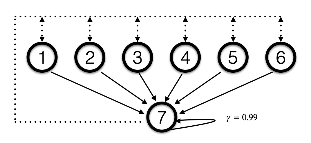
Figure 2: The Baird’s example used in Chapter 11.2 of Sutton & Barto (2018). The figure is taken from Zhang et al. (2020). At each state, there are two actions. The solid action always leads to $s_{7}$; the dashed action leads to one of $\quantity{s_{1},\dots,s_{6}}$ with equal probability. The discount factor $\gamma$ is 0.99.

Figure 2 shows Baird’s example. In the policy evaluation setting (corresponding to Figure 1b), we use the same state features as Sutton & Barto (2018), i.e.,

The weight $w$ is initialized as $[1,1,1,1,1,1,10,1]^{\top}$ as suggested by Sutton & Barto (2018). The behavior policy is $\mu_{0}(\text{dashed}|s_{i})=6/7$ and $\mu_{0}(\text{solid}|s_{i})=1/7$ for $i=1,\dots,7$. And the target policy always selects the solid action. The standard Off-Policy Linear TD (with ridge regularization) updates $w_{t}$ as

$$w_{t+1} \leftarrow w_{t}+\alpha\frac{\pi(A_{t}|S_{t})}{\mu(A_{t}|S_{t})}(R_{t+1}+x_{t+1}^{\top}w_{t}-x_{t}^{\top}w_{t})x_{t}-\alpha\eta w_{t},$$ (279)

where we use $\alpha=0.01$ as used by Sutton & Barto (2018). Note as long as $\alpha>0$, it diverges. Here we overload $x$ to denote the state feature and $x_{t}\doteq x(S_{t})$. We use a TD version of Algorithm 1 to estimate $v_{\pi}$, which updates $w_{t}$ as

$$w_{t+1} \leftarrow w_{t}+\alpha\frac{\pi(A_{t}|S_{t})}{\mu(A_{t}|S_{t})}(R_{t+1}+x_{t+1}^{\top}\theta_{t}-x_{t}^{\top}w_{t})x_{t}-\alpha\eta w_{t},$$ (280)

$$\theta_{t+1} \leftarrow\theta_{t}+\beta(w_{t}-\theta_{t}),$$ (281)

where we set $\alpha=\beta=0.01,\theta_{0}=w_{0}$.

For the control setting (corresponding to Figures 1c & 1d), we construct the state-action feature in the same way as the Errata of Baird (1995), i.e.,

The first 7 rows of $X$ are the features of the solid action; the second 7 rows are the dashed action. The weight $w$ is initialized as $[1,1,1,1,1,1,10,1,1,1,1,1,1,1,1]^{\top}$. The standard linear $Q$-learning (with ridge regularization) updates $w_{t}$ as

$$w_{t+1}\leftarrow w_{t}+\alpha(R_{t+1}+\max_{a^{\prime}}x(S_{t+1},a)^{\top}w_{t}-x_{t}^{\top}w_{t})x_{t}-\alpha\eta w_{t},$$ (282)

where we set $\alpha=0.01$. The variant of Algorithm 3 we use in this experiment updates $w_{t}$ as

$$w_{t+1} \leftarrow w_{t}+\alpha(R_{t+1}+\max_{a^{\prime}}x(S_{t+1},a)^{\top}\theta_{t}-x_{t}^{\top}w_{t})x_{t}-\alpha\eta w_{t},$$ (283)

$$\theta_{t+1} \leftarrow\theta_{t}+\beta(w_{t}-\theta_{t}),$$ (284)

where we set $\alpha=0.01,\beta=0.001,\theta_{0}=w_{0}$. The behavior policy for Figure 1c is still $\mu_{0}$; the behavior policy for Figure 1d is $0.9\mu_{0}+0.1\mu_{w}$, where $\mu_{w}$ is a softmax policy w.r.t. $x(s,\cdot)^{\top}w$. For our algorithm with target network, the softmax policy is computed using the target network as shown in Algorithm 3.

References

• Achiam et al. (2019) Achiam, J., Knight, E., and Abbeel, P. Towards characterizing divergence in deep q-learning. arXiv preprint arXiv:1903.08894, 2019.
• Baird (1995) Baird, L. Residual algorithms: Reinforcement learning with function approximation. Machine Learning, 1995.
• Borkar (2009) Borkar, V. S. Stochastic approximation: a dynamical systems viewpoint. Springer, 2009.
• Boyan (1999) Boyan, J. A. Least-squares temporal difference learning. In Proceedings of the 16th International Conference on Machine Learning, 1999.
• Cai et al. (2019) Cai, Q., Yang, Z., Lee, J. D., and Wang, Z. Neural temporal-difference and q-learning provably converge to global optima. arXiv preprint arXiv:1905.10027, 2019.
• Carvalho et al. (2020) Carvalho, D., Melo, F. S., and Santos, P. A new convergent variant of q-learning with linear function approximation. Advances in Neural Information Processing Systems, 33, 2020.
• Chen et al. (2019a) Chen, S., Devraj, A. M., Bušić, A., and Meyn, S. Zap q-learning with nonlinear function approximation. arXiv preprint arXiv:1910.05405, 2019a.
• Chen et al. (2019b) Chen, Z., Zhang, S., Doan, T. T., Clarke, J.-P., and Maguluri, S. T. Finite-sample analysis of nonlinear stochastic approximation with applications in reinforcement learning. arXiv preprint arXiv:1905.11425, 2019b.
• Diddigi et al. (2019) Diddigi, R. B., Kamanchi, C., and Bhatnagar, S. A convergent off-policy temporal difference algorithm. arXiv preprint arXiv:1911.05697, 2019.
• Du et al. (2017) Du, S. S., Chen, J., Li, L., Xiao, L., and Zhou, D. Stochastic variance reduction methods for policy evaluation. In Proceedings of the 34th International Conference on Machine Learning, 2017.
• Du et al. (2019) Du, S. S., Luo, Y., Wang, R., and Zhang, H. Provably efficient q-learning with function approximation via distribution shift error checking oracle. In Advances in Neural Information Processing Systems, 2019.
• Du et al. (2020) Du, S. S., Lee, J. D., Mahajan, G., and Wang, R. Agnostic $q$-learning with function approximation in deterministic systems: Near-optimal bounds on approximation error and sample complexity. Advances in Neural Information Processing Systems, 2020.
• Dulac-Arnold et al. (2019) Dulac-Arnold, G., Mankowitz, D., and Hester, T. Challenges of real-world reinforcement learning. arXiv preprint arXiv:1904.12901, 2019.
• Fan et al. (2020) Fan, J., Wang, Z., Xie, Y., and Yang, Z. A theoretical analysis of deep q-learning. In Learning for Dynamics and Control. PMLR, 2020.
• Fujimoto et al. (2018) Fujimoto, S., van Hoof, H., and Meger, D. Addressing function approximation error in actor-critic methods. arXiv preprint arXiv:1802.09477, 2018.
• Haarnoja et al. (2018) Haarnoja, T., Zhou, A., Abbeel, P., and Levine, S. Soft actor-critic: Off-policy maximum entropy deep reinforcement learning with a stochastic actor. arXiv preprint arXiv:1801.01290, 2018.
• Jin et al. (2020) Jin, C., Yang, Z., Wang, Z., and Jordan, M. I. Provably efficient reinforcement learning with linear function approximation. In Conference on Learning Theory, pp.  2137–2143. PMLR, 2020.
• Johns et al. (2010) Johns, J., Painter-Wakefield, C., and Parr, R. Linear complementarity for regularized policy evaluation and improvement. Advances in neural information processing systems, 2010.
• Kolter (2011) Kolter, J. Z. The fixed points of off-policy td. In Advances in Neural Information Processing Systems, 2011.
• Kolter & Ng (2009) Kolter, J. Z. and Ng, A. Y. Regularization and feature selection in least-squares temporal difference learning. In Proceedings of the 26th annual international conference on machine learning, 2009.
• Konda (2002) Konda, V. R. Actor-critic algorithms. PhD thesis, Massachusetts Institute of Technology, 2002.
• Kushner & Yin (2003) Kushner, H. and Yin, G. G. Stochastic approximation and recursive algorithms and applications. Springer Science & Business Media, 2003.
• Lee & He (2019) Lee, D. and He, N. A unified switching system perspective and ode analysis of q-learning algorithms. arXiv preprint arXiv:1912.02270, 2019.
• Li et al. (2011) Li, L., Littman, M. L., Walsh, T. J., and Strehl, A. L. Knows what it knows: a framework for self-aware learning. Machine learning, 2011.
• Lillicrap et al. (2015) Lillicrap, T. P., Hunt, J. J., Pritzel, A., Heess, N., Erez, T., Tassa, Y., Silver, D., and Wierstra, D. Continuous control with deep reinforcement learning. arXiv preprint arXiv:1509.02971, 2015.
• Lin (1992) Lin, L.-J. Self-improving reactive agents based on reinforcement learning, planning and teaching. Machine Learning, 1992.
• Liu et al. (2012) Liu, B., Mahadevan, S., and Liu, J. Regularized off-policy td-learning. Advances in Neural Information Processing Systems, 2012.
• Maei et al. (2010) Maei, H. R., Szepesvári, C., Bhatnagar, S., and Sutton, R. S. Toward off-policy learning control with function approximation. In Proceedings of the 27th International Conference on Machine Learning, 2010.
• Marbach & Tsitsiklis (2001) Marbach, P. and Tsitsiklis, J. N. Simulation-based optimization of markov reward processes. IEEE Transactions on Automatic Control, 2001.
• Melo et al. (2008) Melo, F. S., Meyn, S. P., and Ribeiro, M. I. An analysis of reinforcement learning with function approximation. In Proceedings of the 25th International Conference on Machine Learning, 2008.
• Mnih et al. (2015) Mnih, V., Kavukcuoglu, K., Silver, D., Rusu, A. A., Veness, J., Bellemare, M. G., Graves, A., Riedmiller, M., Fidjeland, A. K., Ostrovski, G., et al. Human-level control through deep reinforcement learning. Nature, 2015.
• Painter-Wakefield et al. (2012) Painter-Wakefield, C., Parr, R., and Durham, N. L1 regularized linear temporal difference learning. Technical report: Department of Computer Science, Duke University, Durham, NC, TR-2012–01, 2012.
• Petrik et al. (2010) Petrik, M., Taylor, G., Parr, R., and Zilberstein, S. Feature selection using regularization in approximate linear programs for markov decision processes. arXiv preprint arXiv:1005.1860, 2010.
• Puterman (2014) Puterman, M. L. Markov decision processes: discrete stochastic dynamic programming. John Wiley & Sons, 2014.
• Silver et al. (2016) Silver, D., Huang, A., Maddison, C. J., Guez, A., Sifre, L., Van Den Driessche, G., Schrittwieser, J., Antonoglou, I., Panneershelvam, V., Lanctot, M., et al. Mastering the game of go with deep neural networks and tree search. Nature, 2016.
• Sutton (1988) Sutton, R. S. Learning to predict by the methods of temporal differences. Machine Learning, 1988.
• Sutton & Barto (2018) Sutton, R. S. and Barto, A. G. Reinforcement Learning: An Introduction (2nd Edition). MIT press, 2018.
• Sutton et al. (2009a) Sutton, R. S., Maei, H. R., Precup, D., Bhatnagar, S., Silver, D., Szepesvári, C., and Wiewiora, E. Fast gradient-descent methods for temporal-difference learning with linear function approximation. In Proceedings of the 26th International Conference on Machine Learning, 2009a.
• Sutton et al. (2009b) Sutton, R. S., Maei, H. R., and Szepesvári, C. A convergent $o(n)$ temporal-difference algorithm for off-policy learning with linear function approximation. In Advances in Neural Information Processing Systems, 2009b.
• Sutton et al. (2011) Sutton, R. S., Modayil, J., Delp, M., Degris, T., Pilarski, P. M., White, A., and Precup, D. Horde: A scalable real-time architecture for learning knowledge from unsupervised sensorimotor interaction. In Proceedings of the 10th International Conference on Autonomous Agents and Multiagent Systems, 2011.
• Sutton et al. (2016) Sutton, R. S., Mahmood, A. R., and White, M. An emphatic approach to the problem of off-policy temporal-difference learning. The Journal of Machine Learning Research, 2016.
• Szepesvári & Smart (2004) Szepesvári, C. and Smart, W. D. Interpolation-based q-learning. In Proceedings of the twenty-first international conference on Machine learning, pp.  100, 2004.
• Tikhonov et al. (2013) Tikhonov, A. N., Goncharsky, A., Stepanov, V., and Yagola, A. G. Numerical methods for the solution of ill-posed problems. Springer Science & Business Media, 2013.
• Tsitsiklis & Van Roy (1996) Tsitsiklis, J. N. and Van Roy, B. Feature-based methods for large scale dynamic programming. Machine Learning, 1996.
• Tsitsiklis & Van Roy (1997) Tsitsiklis, J. N. and Van Roy, B. Analysis of temporal-diffference learning with function approximation. In Advances in Neural Information Processing Systems, 1997.
• Van Hasselt et al. (2018) Van Hasselt, H., Doron, Y., Strub, F., Hessel, M., Sonnerat, N., and Modayil, J. Deep reinforcement learning and the deadly triad. arXiv preprint arXiv:1812.02648, 2018.
• Vidyasagar (2002) Vidyasagar, M. Nonlinear systems analysis. SIAM, 2002.
• Wan et al. (2020) Wan, Y., Naik, A., and Sutton, R. S. Learning and planning in average-reward markov decision processes. arXiv preprint arXiv:2006.16318, 2020.
• Wang & Zou (2020) Wang, Y. and Zou, S. Finite-sample analysis of greedy-gq with linear function approximation under markovian noise. arXiv preprint arXiv:2005.10175, 2020.
• Wang et al. (2019) Wang, Y., Wang, R., Du, S. S., and Krishnamurthy, A. Optimism in reinforcement learning with generalized linear function approximation. arXiv preprint arXiv:1912.04136, 2019.
• Watkins & Dayan (1992) Watkins, C. J. and Dayan, P. Q-learning. Machine Learning, 1992.
• Wen & Van Roy (2013) Wen, Z. and Van Roy, B. Efficient exploration and value function generalization in deterministic systems. Advances in Neural Information Processing Systems, 2013.
• Wu et al. (2020) Wu, Y., Zhang, W., Xu, P., and Gu, Q. A finite time analysis of two time-scale actor critic methods. arXiv preprint arXiv:2005.01350, 2020.
• Xu & Gu (2020) Xu, P. and Gu, Q. A finite-time analysis of q-learning with neural network function approximation. In International Conference on Machine Learning, pp. 10555–10565. PMLR, 2020.
• Yang & Wang (2020) Yang, L. and Wang, M. Reinforcement learning in feature space: Matrix bandit, kernels, and regret bound. In International Conference on Machine Learning, pp. 10746–10756. PMLR, 2020.
• Yang & Wang (2019) Yang, L. F. and Wang, M. Sample-optimal parametric q-learning using linearly additive features. arXiv preprint arXiv:1902.04779, 2019.
• Yang et al. (2019) Yang, Z., Fu, Z., Zhang, K., and Wang, Z. Convergent reinforcement learning with function approximation: A bilevel optimization perspective, 2019. URL https://openreview.net/forum?id=ryfcCo0ctQ.
• Yu (2010) Yu, H. Convergence of least squares temporal difference methods under general conditions. In ICML, 2010.
• Yu (2017) Yu, H. On convergence of some gradient-based temporal-differences algorithms for off-policy learning. arXiv preprint arXiv:1712.09652, 2017.
• Zhang et al. (2020) Zhang, S., Liu, B., Yao, H., and Whiteson, S. Provably convergent two-timescale off-policy actor-critic with function approximation. In Proceedings of the 37th International Conference on Machine Learning, 2020.
• Zhang et al. (2021) Zhang, S., Wan, Y., Sutton, R. S., and Whiteson, S. Average-reward off-policy policy evaluation with function approximation. arXiv preprint arXiv:2101.02808, 2021.
• Zou et al. (2019) Zou, S., Xu, T., and Liang, Y. Finite-sample analysis for sarsa with linear function approximation. In Advances in Neural Information Processing Systems, 2019.