Fixed-Domain Asymptotics Under Vecchia’s Approximation of Spatial Process Likelihoods

Abstract

Statistical modeling for massive spatial data sets has generated a substantial literature on scalable spatial processes based upon Vecchia’s approximation. Vecchia’s approximation for Gaussian process models enables fast evaluation of the likelihood by restricting dependencies at a location to its neighbors. We establish inferential properties of microergodic spatial covariance parameters within the paradigm of fixed-domain asymptotics when they are estimated using Vecchia’s approximation. The conditions required to formally establish these properties are explored, theoretically and empirically, and the effectiveness of Vecchia’s approximation is further corroborated from the standpoint of fixed-domain asymptotics.

Keywords: Fixed-domain asymptotics; Gaussian processes; Likelihood approximations; Matérn covariance function; Microergodic parameter estimation; Spatial statistics

I.   Introduction

Geostatististical data are often modeled by treating observations as partial realizations of a spatial random field. We customarily model the random field $\{Y(s):s\in{\cal D}\}$ over a bounded region ${\cal D}\in\mathbb{R}^{d}$ as a Gaussian process (GP), denoted $Y(s)\sim GP(\mu_{\beta}(s),K_{\theta}(\cdot,\cdot))$, with mean $\mu_{\beta}(s)$ and covariance function $K_{\theta}(s,s^{\prime})=\mbox{cov}(y(s_{i}),y(s_{j}))$. The probability law for a finite set $\chi=\{s_{1},s_{2},\ldots,s_{n}\}$ is given by $y\sim N(\mu_{\beta},K_{\theta})$, where $y=(y(s_{i}))$ and $\mu_{\beta}=(\mu_{\beta}(s_{i}))$ are $n\times 1$ vectors with elements $y(s_{i})$ and $\mu_{\beta}(s_{i})$, respectively, and $K_{\theta}=(K_{\theta}(s_{i},s_{j}))$ is the $n\times n$ spatial covariance matrix whose $(i,j)$th element is the value of the covariance function $K_{\theta}(s_{i},s_{j})$. We consider the widely employed stationary Matérn covariance function (Matérn, 1986; Stein, 1999b) given by

$$K_{\theta}(s,s^{\prime}):=\frac{\sigma^{2}(\phi\|h\|)^{\nu}}{\Gamma(\nu)2^{\nu-1}}{\cal K}_{\nu}(\phi\|h\|),\quad\|h\|\geq 0\;,$$ (1)

where $h=s-s^{\prime}$, $\sigma^{2}>0$ is called the partial sill or spatial variance, $\phi>0$ is the scale or decay parameter, $\nu>0$ is a smoothness parameter, $\Gamma(\cdot)$ is the Gamma function, ${\cal K}_{\nu}(\cdot)$ is the modified Bessel function of order $\nu$ (Abramowitz and Stegun, 1965, Section 10) and $\theta=\{\sigma^{2},\phi,\nu\}$. The spectral density corresponding to (1), which we will need later, is

$$f(u)=C\frac{\sigma^{2}\phi^{2\nu}}{(\phi^{2}+u^{2})^{\nu+\frac{d}{2}}}\quad\mbox{for some }C>0.$$ (2)

Likelihood-based inference for $\theta$ will require matrix computations in the order of $\sim n^{3}$ floating point operations (flops) and can become impracticable when the number of spatial locations, $n$, is very large. Writing $Y_{n}=(y_{1},y_{2},\ldots,y_{n})^{\top}$, where $y_{i}:=y(s_{i})$ for $i=1,2,\ldots,n$ are the $n$ sampled measurements, we write the joint density $p(Y_{n}\,|\,\theta):=N(Y_{n};\;\mu_{\beta},K_{\theta})$ as

$$p(Y_{n}\,|\,\theta)=p(y_{1};\theta)\prod_{i=2}^{n}p(y_{i}\,|\,y_{(i-1)};\theta)\;,$$ (3)

where $y_{(i)}=(y_{1},\ldots y_{i})$. Vecchia (1988) suggested a simple approximation to (3) based upon the notion that it may not be critical to use all components of $y_{(i-1)}$ in $p(y_{i}\,|\,y_{(i-1)};\theta)$. Instead, the joint density $p(Y_{n}\,|\,\theta)$ in (3) is approximated by

$$\tilde{p}(Y_{n}\,|\,\theta)=p(y_{1}\,|\,\theta)\prod_{i=2}^{n}p(y_{i}\,|\,S_{(i-1)};\theta)\;,$$ (4)

where $S_{(i)}$ is a subvector of $y_{(i)}$ for $i=1,\ldots,n$. The density $\tilde{p}(Y_{n}\,|\,\theta)$ in (4) is called Vecchia’s approximation and can be regarded as a quasi- or composite likelihood (Zhang, 2012; Eidsvik et al., 2014; Bachoc and Lagnoux, 2020). Vecchia’s approximation has attracted a remarkable amount of attention in recent times, already too vast to be comprehensively reviewed here (see, e.g., Stein et al., 2004; Datta et al., 2016a, b; Guinness, 2018; Katzfuss et al., 2020; Katzfuss and Guinness, 2021; Peruzzi et al., 2022). Algorithmic developments in Bayesian and frequentist settings Finley et al. (2019); Zhang et al. (2019); Katzfuss et al. (2020) have enabled scalability to massive data sets (with $n\sim 10^{7}$ locations) and (4) lies at the core of several methods that tackle “big data” problems in geospatial analysis (Sun et al., 2012; Banerjee, 2017; Heaton et al., 2019).

The Vecchia approximation has recently garnered substantial attention in the spatial statistics literature as an edifice for building massively scalable Gaussian process models. While substantial methodological innovation has been generated by this approach, developing a theoretical understanding regarding the inference and identifiability of the spatial process parameters has remained largely unaddressed. This is because the Vecchia approximation distorts the stationarity of the parent process and, hence, the theoretical tractability of the spatial processes are lost. Our current approach is an original first attempt based upon Zhang (2012) to formally introduce methods that can study the asymptotic properties of inference from Vecchia’s approximation. While a completely rigorous development is available only in the one-dimensional setting, we emphasize that the approach we develop is novel and should generate subsequent theoretical research in two-dimensions. Therefore, we limit the formal theory to one-dimension but present some insightful numerical experiments in two-dimensions to show that the inferential behavior secured over the real line will be expected to carry over to spatial domains.

Following the fixed-domain (infill) asymptotic paradigm for spatial inference (Stein, 1999a; Zhang and Zimmerman, 2005) we discuss inferential properties for the parameters in (1). In this setting, Zhang (2004) showed that not all parameters in $\theta$ admit consistent maximum likelihood estimators from the full Gaussian likelihood in (3) constructed with a stationary Matérn covariance function, but certain microergodic parameters are consistently estimated. Du et al. (2009, Theorem 5) formally established the asymptotic distributions of these microergodic parameters. Kaufman and Shaby (2013) addressed jointly estimating the decay and the variance parameters in the Matérn family and the effect of a prefixed decay on inference when having relatively small sample size. All of the aforementioned work has been undertaken using (3). Here, we formally establish the inferential properties for the estimates of microergodic parameters obtained from Vecchia’s approximate likelihood in (4). We build our work on a brief but insightful discussion in Section 10.5.3 of Zhang (2012), regarding the inferential behaviour arising from (4). To the best of our knowledge such explorations have not hitherto been formally undertaken. Following the aforementioned works in spatial asymptotics, we will restrict attention to the infill or fixed domain setting and focus on the inferential properties of the microergodic parameters for any given value of the smoothness parameter. More specifically, we explore the criteria for asymptotic normality for the maximum likelihood estimates of the microergodic parameters obtained from Vecchia’s approximation. In this regard, our work follows the paradigm laid out in Zhang (2012) in that we can no longer assume that the conditioning set is bounded. We provide conditions under which the inference under the Vecchia approximations of the Matérn process will be asymptotically equivalent to the full model. This distinguishes our intended contribution from that in Bachoc and Lagnoux (2020), where bounded conditional sets are exploited to establish consistency results for some selected values of the smoothness parameter. On the other hand, we show that a different set of conditions can yield a closed form asymptotic distribution for any given value of the smoothness parameter. For the subsequent development, it suffices to assume that $\mu_{\beta}(s)=0$, i.e., the data has been detrended. Hence, we work with a zero-centered stationary Gaussian process with the Matérn covariance function in (1), a fixed smoothness parameter $\nu$ and with the sampling locations $\chi_{n}$ restricted to a bounded region.

The balance of this article is arranged as follows. One of our key results, Theorem 1, is presented in Section II, providing general criteria for asymptotic normality of maximum likelihood estimates of microergodic parameters obtained from Vecchia’s approximation. In Section III, we demonstrate that these general criteria are implied by a condition on the conditioning size which grows much slower than the sample size. We numerically check the conclusions for one-dimensional cases and extend the discussion for two-dimensional cases in Section IV.

II.   Infill Asymptotics for Vecchia’s approximation

II.1   Microergodic parameters

Identifiability and consistent estimation of $\theta$ in (1) relies upon the equivalence and orthogonality of Gaussian measures. Two probability measures $P_{1}$ and $P_{2}$ on a measurable space $(\Omega,{\cal F})$ are said to be equivalent, denoted $P_{1}\equiv P_{2}$, if they are absolutely continuous with respect to each other. Thus, $P_{1}\equiv P_{2}$ implies that for all $A\in{\cal F}$, $P_{1}(A)=0$ if and only if $P_{2}(A)=0$. On the other hand, $P_{1}$ and $P_{2}$ are orthogonal, denoted $P_{1}\perp P_{2}$, if there exists $A\in{\cal F}$ for which $P_{1}(A)=1$ and $P_{2}(A)=0$. While measures may be neither equivalent nor orthogonal, Gaussian measures are in general one or the other. For a Gaussian probability measure $P_{\theta}$ indexed by a set of parameters $\theta$ and $\kappa$, a function of $\theta$, we say that $\kappa(\theta)$ is microergodic if $\kappa(\theta_{1})\neq\kappa(\theta_{2})$ implies $P_{\theta_{1}}\perp P_{\theta_{2}}$ (see, e.g., Stein, 1999b; Zhang, 2012). Two Gaussian probability measures defined by Matérn covariance functions $K_{\theta_{1}}(h)$ and $K_{\theta_{2}}(h)$, where $\theta_{1}=\{\sigma^{2}_{1},\phi_{1},\nu\}$ and $\theta_{2}=\{\sigma^{2}_{2},\phi_{2},\nu\}$ are equivalent if and only if $\sigma_{1}^{2}\phi_{1}^{2\nu}=\sigma_{2}^{2}\phi_{2}^{2\nu}$ (Theorem 2 in Zhang, 2004). Consequently, one cannot consistently estimate $\sigma^{2}$ or $\phi$ (Corollary 1 in Zhang, 2004) from full Gaussian process likelihood functions, $\sigma^{2}\phi^{2\nu}$ is a microergodic parameter that can be consistently estimated.

If the oracle (data generating) values of $\phi$ and $\sigma^{2}$ are $\phi_{0}$ and $\sigma^{2}_{0}$, respectively, then for any fixed value of the decay $\phi=\phi_{1}$, we know from Du et al. (2009, Theorem 5) that

$$\sqrt{n}(\hat{\sigma}_{n}^{2}\phi_{1}^{2\nu}-\sigma_{0}^{2}\phi_{0}^{2\nu})\overset{{\cal L}}{\longrightarrow}N(0,2(\sigma_{0}^{2}\phi_{0}^{2\nu})^{2})\;,$$ (5)

where $\hat{\sigma}_{n}^{2}$ is the maximum likelihood estimator from the full likelihood (3).

II.2   Parameter estimation

Let $\hat{\sigma}_{n,vecch}^{2}$ be the maximum likelihood estimate of the variance $\sigma^{2}$,

$$\hat{\sigma}_{n,vecch}^{2}=\mbox{argmax}_{\sigma^{2}}\{\tilde{p}(Y_{n}\,|\,\phi_{1},\sigma^{2}),\;\sigma^{2}\in\mathbb{R}^{+}\}\;,$$ (6)

where $\tilde{p}(\cdot)$ is the density (4). We develop the asymptotic equivalence of $\hat{\sigma}_{n,vecch}^{2}$ with $\hat{\sigma}_{n}^{2}$. To proceed further, we introduce some notations. Assume that the target process $y(s)\sim GP(0,K_{\theta}(\cdot))$, where $K_{\theta}(h)$ is defined in (1) with a fixed $\nu$. Let $P_{j}$, $j=0,1$ denote probability measures for $y(s)\sim GP(0,K_{\theta_{i}})$ with $\theta_{j}=\{\sigma_{j}^{2},\phi_{j},\nu\}$. Assume that $\sigma_{1}^{2}=\sigma_{0}^{2}\phi_{0}^{2\nu}/\phi_{1}^{2\nu}$ and let $E_{j}(\cdot)$ denote the expectation with respect to probability measure $P_{j}$, $j=0,1$. We define

$$\begin{split}e_{0,j}&:=y_{1},\;\mu_{i,j}:=E_{j}(y_{i}\,|\,y_{(i-1)}),\;e_{i,j}:=y_{i}-\mu_{i,j},\;i=2,\ldots,n\\ \tilde{e}_{0,j}&:=y_{1},\;\tilde{\mu}_{i,j}:=E_{j}(y_{i}\,|\,S_{(i-1)}),\;\tilde{e}_{i,j}:=y_{i}-\tilde{\mu}_{i,j},\;i=2,\ldots,n\;.\end{split}$$ (7)

In Lemma 1 we derive a useful expression for $\hat{\sigma}_{n,vecch}^{2}$ using the quantities in (7).

Lemma 1.

The estimate of $\sigma^{2}$ from Vecchia’s likelihood approximation with fixed $\nu$, and $\phi=\phi_{1}$ can be expressed as

$$\hat{\sigma}^{2}_{n,vecch}=\frac{\sigma_{1}^{2}}{n}\sum_{i=1}^{n}\frac{\tilde{e}_{i,1}^{2}}{E_{1}\tilde{e}_{i,1}^{2}}\;.$$ (8)

Proof.

In Vecchia’s approximation (4) with fixed $\nu$, $\phi=\phi_{1}$ and unknown $\sigma^{2}$ in $K_{\theta}(\cdot)$, $p(y_{i}\,|\,S_{(i-1)})$ is Gaussian with mean $\widetilde{\mu}_{i,1}=\widetilde{\Sigma}_{i,1}^{12}(\widetilde{\Sigma}_{i,1}^{22})^{-1}S_{(i-1)}$ and variance $\widetilde{\Sigma}_{i,1}:=\widetilde{\Sigma}_{i,1}^{11}-\widetilde{\Sigma}_{i,1}^{12}(\widetilde{\Sigma}_{i,1}^{22})^{-1}\widetilde{\Sigma}_{i,1}^{21}$, where $\displaystyle\begin{pmatrix}\widetilde{\Sigma}_{i,1}^{11}&\widetilde{\Sigma}_{i,1}^{12}\\ \widetilde{\Sigma}_{i,1}^{21}&\widetilde{\Sigma}_{i,1}^{22}\end{pmatrix}$ is the covariance matrix of $\displaystyle\begin{pmatrix}y_{i}\\ S_{(i-1)}\end{pmatrix}$ under $\tilde{p}(\cdot;\phi_{1},\sigma^{2})$. Since $\widetilde{\mu}_{i,1}$ does not depend on $\sigma^{2}$, and $\widetilde{\Sigma}_{i,1}$ can be expressed as $\sigma^{2}\widetilde{\Sigma}^{\dagger}_{i,1}$, where $\widetilde{\Sigma}^{\dagger}_{i,1}$ does not depend upon $\sigma^{2}$, the conditional distributions $p(y_{i}\,|\,S_{(i-1)})$ under Vecchia’s approximation is

$$p(y_{i}\,|\,S_{(i-1)})=\frac{1}{\sqrt{2\pi\sigma^{2}\widetilde{\Sigma}^{\dagger}_{i,1}}}\exp\left(-\frac{\tilde{e}_{i,1}^{2}}{2\sigma^{2}\widetilde{\Sigma}^{\dagger}_{i,1}}\right).$$

A direct computation of (6) with any fixed $\phi_{1}$ yields (8), where we have used the fact $E_{1}\tilde{e}^{2}_{i,1}=\sigma_{1}^{2}\widetilde{\Sigma}^{\dagger}_{i,1}$ on the right hand side of (8). ∎

Our main result builds on the discussion in Section 10.5.3 of Zhang (2012) to establish the following theorem that explores the asymptotic distribution of $\hat{\sigma}_{n,vecch}^{2}$.

Theorem 1.

Assume that either of the following conditions holds:

$$\sum_{i=1}^{n}\frac{E_{0}(\tilde{e}_{i,1}-e_{i,0})^{2}}{E_{1}\tilde{e}_{i,1}^{2}}=\mathcal{O}(1)\quad\mbox{and}\quad\sum_{i=1}^{n}\left(\frac{E_{0}e_{i,0}^{2}}{E_{1}\tilde{e}_{i,1}^{2}}-1\right)^{2}=\mathcal{O}(1).$$ (9)

or

$$\sum_{i=1}^{n}\frac{E_{1}(\tilde{e}_{i,1}-e_{i,0})^{2}}{E_{0}e_{i,0}^{2}}=\mathcal{O}(1)\quad\mbox{and}\quad\sum_{i=1}^{n}\left(\frac{E_{1}\tilde{e}_{i,1}^{2}}{E_{0}e_{i,0}^{2}}-1\right)^{2}=\mathcal{O}(1).$$ (10)

Then

$$\sqrt{n}(\hat{\sigma}_{n,vecch}^{2}\phi_{1}^{2\nu}-\sigma_{0}^{2}\phi_{0}^{2\nu})\overset{\mathcal{L}}{\longrightarrow}N(0,2(\sigma_{0}^{2}\phi_{0}^{2\nu})^{2})\;.$$ (11)

Before presenting the proof of Theorem 1, we state and prove the following lemma.

Lemma 2.

The assumptions in (9) imply that

$$E_{0}\left[\sum_{i=1}^{n}\frac{\tilde{e}_{i,1}^{2}}{E_{1}\tilde{e}_{i,1}^{2}}-\sum_{i=1}^{n}\frac{e_{i,0}^{2}}{E_{0}e_{i,0}^{2}}\right]=o(\sqrt{n}),$$ (12)

Proof.

We first prove that (9) implies (12). Note that

$$\Bigg{|}E_{0}\left[\sum_{i=1}^{n}\frac{\tilde{e}_{i,1}^{2}}{E_{1}\tilde{e}_{i,1}^{2}}-\sum_{i=1}^{n}\frac{e_{i,0}^{2}}{E_{0}e_{i,0}^{2}}\right]\Bigg{|} =\Bigg{|}\sum_{i=1}^{n}\left(\frac{E_{0}(\tilde{e}_{i,1}-e_{i,0}+e_{i,0})^{2}}{E_{1}\tilde{e}_{i,1}^{2}}-1\right)\Bigg{|}$$

$$=\Bigg{|}\sum_{i=1}^{n}\frac{E_{0}(\tilde{e}_{i,1}-e_{i,0})^{2}}{E_{1}\tilde{e}_{i,1}^{2}}+\sum_{i=1}^{n}\left(\frac{E_{0}e_{i,0}^{2}}{E_{1}\tilde{e}_{i,1}^{2}}-1\right)\Bigg{|}$$

$$\leq\sum_{i=1}^{n}\frac{E_{0}(\tilde{e}_{i,1}-e_{i,0})^{2}}{E_{1}\tilde{e}_{i,1}^{2}}+\sum_{i=1}^{n}\Bigg{|}\frac{E_{0}e_{i,0}^{2}}{E_{1}\tilde{e}_{i,1}^{2}}-1\Bigg{|},$$

where the second equality follows from the fact that $\tilde{e}_{i,1}-e_{i,0}$ and $e_{i,0}$ are independent under $P_{0}$. By the first condition in (9), we get $\sum_{i=1}^{n}E_{0}(\tilde{e}_{i,1}-e_{i,0})^{2}/E_{1}\tilde{e}_{i,1}^{2}=\mathcal{O}(1)=o(\sqrt{n})$. Fix $\varepsilon>0$. By the second condition in (9), there is $M>0$ such that $\sum_{i>M}\left(E_{0}e_{i,0}^{2}/E_{1}\tilde{e}_{i,1}^{2}-1\right)^{2}<\varepsilon$. So for $n>M$, we can use the Cauchy–Schwarz inequality to obtain

$$\sum_{i=1}^{n}\left|\frac{E_{0}e_{i,0}^{2}}{E_{1}\tilde{e}_{i,1}^{2}}-1\right| =\sum_{i=1}^{M}\left|\frac{E_{0}e_{i,0}^{2}}{E_{1}\tilde{e}_{i,1}^{2}}-1\right|+\sum_{i=M+1}^{n}\left|\frac{E_{0}e_{i,0}^{2}}{E_{1}\tilde{e}_{i,1}^{2}}-1\right|$$

$$\leq\sum_{i=1}^{M}\left|\frac{E_{0}e_{i,0}^{2}}{E_{1}\tilde{e}_{i,1}^{2}}-1\right|+\sqrt{(n-M)\varepsilon}\;.$$

Dividing both sides by $\sqrt{n}$ reveals that $\limsup_{n\rightarrow\infty}\frac{1}{\sqrt{n}}\sum_{i=1}^{n}\left|E_{0}e_{i,0}^{2}/E_{1}\tilde{e}_{i,1}^{2}-1\right|\leq\sqrt{\varepsilon}$. Since $\varepsilon>0$ is arbitrary, it follows that $\sum_{i=1}^{n}\left|E_{0}e_{i,0}^{2}/E_{1}\tilde{e}_{i,1}^{2}-1\right|=o(\sqrt{n})$ and we obtain (12).

∎

We now present a proof of Theorem 1.

Proof of Theorem 1.

Recall that $\sum_{i=1}^{n}e_{i,0}^{2}/(E_{0}e_{i,0}^{2})=Y_{n}^{\top}V_{n,0}^{-1}Y_{n}$, where $V_{n,0}$ is the covariance matrix of $Y_{n}$ under $P_{0}$. Using (8) that was derived in Lemma 1, we obtain

$$\sqrt{n}(\hat{\sigma}_{n,vecch}^{2}/\sigma_{1}^{2}-1)=\frac{1}{\sqrt{n}}\left[\sum_{i=1}^{n}\frac{\tilde{e}_{i,1}^{2}}{E_{1}\tilde{e}_{i,1}^{2}}-\sum_{i=1}^{n}\frac{e_{i,0}^{2}}{E_{0}e_{i,0}^{2}}\right]+\sqrt{n}\left(\frac{1}{n}Y_{n}^{\top}V_{n,0}^{-1}Y_{n}-1\right).$$ (13)

By the central limit theorem, we have $\sqrt{n}\left(\frac{1}{n}Y_{n}^{\top}V_{n,0}^{-1}Y_{n}-1\right)\overset{\mathcal{L}}{\longrightarrow}N(0,2)$.

We next show that the condition (9) implies that

$$\begin{split}\sum_{i=1}^{n}\frac{\tilde{e}_{i,1}^{2}}{E_{1}\tilde{e}_{i,1}^{2}}-\sum_{i=1}^{n}\frac{e_{i,0}^{2}}{E_{0}e_{i,0}^{2}}&=o(\sqrt{n}).\end{split}$$ (14)

To prove this, it will be sufficient to show that

$$\sum_{i=1}^{n}\frac{\tilde{e}_{i,1}^{2}}{E_{1}\tilde{e}_{i,1}^{2}}-\sum_{i=1}^{n}\frac{e_{i,0}^{2}}{E_{0}e_{i,0}^{2}}-E_{0}\left[\sum_{i=1}^{n}\frac{\tilde{e}_{i,1}^{2}}{E_{1}\tilde{e}_{i,1}^{2}}-\sum_{i=1}^{n}\frac{e_{i,0}^{2}}{E_{0}e_{i,0}^{2}}\right]=O(1).$$ (15)

The result in (14) will then follow from Lemma 2. We turn to proving (15). Our argument relies on the equivalence of Gaussian sequences. Let $\widetilde{P}_{1,n}$ be the probability distribution corresponding to $\tilde{p}(Y_{n};\phi_{1},\sigma_{1}^{2})$, and let $\rho_{n}:=\tilde{p}(Y_{n};\phi_{1},\sigma_{1}^{2})/p(Y_{n};\phi_{0},\sigma_{0}^{2})$ be the Radon-Nikodym derivative of $\widetilde{P}_{1,n}$ with respect to $P_{0}$ on the realization $Y_{n}$ for a given $n$. Write $\widetilde{P}_{1,\infty}$ (respectively, $P_{0,\infty}$) for the probability distribution corresponding to $\tilde{p}(\cdot;\phi_{1},\sigma_{1}^{2})$ (respectively, $p(\cdot;\phi_{0},\sigma_{0}^{2})$) on the infinite sequence $(Y_{1},Y_{2},\ldots)$. By Kakutani’s dichotomy, $\widetilde{P}_{1,\infty}$ and $P_{0,\infty}$ are either equivalent or mutually singular to each other. If $\widetilde{P}_{1,\infty}$ is equivalent to $P_{0,\infty}$, then $\mbox{lim}_{n\rightarrow\infty}\rho_{n}=\rho_{\infty}=:d\widetilde{P}_{1,\infty}/dP_{0,\infty}$ with $P_{0}$-probability $1$ (see, e.g., Ibragimov and Rozanov, 1978, Section III.2.1). Also, $\mathbb{P}_{0}(0<\rho_{\infty}<\infty)=1$ and $-\infty<E_{0}(\log\rho_{\infty})<\infty$. As a consequence,

$$\log\rho_{n} =-\frac{1}{2}\log\frac{\det\widetilde{V}_{n,1}}{\det V_{n,0}}-\frac{1}{2}\left(\sum_{i=1}^{n}\frac{\tilde{e}_{i,1}^{2}}{E_{1}\tilde{e}_{i,1}^{2}}-\sum_{i=1}^{n}\frac{e_{i,0}^{2}}{E_{0}e_{i,0}^{2}}\right)=\mathcal{O}(1),$$

$$E_{0}(\log\rho_{n}) =-\frac{1}{2}\log\frac{\det\widetilde{V}_{n,1}}{\det V_{n,0}}-\frac{1}{2}E_{0}\left[\sum_{i=1}^{n}\frac{\tilde{e}_{i,1}^{2}}{E_{1}\tilde{e}_{i,1}^{2}}-\sum_{i=1}^{n}\frac{e_{i,0}^{2}}{E_{0}e_{i,0}^{2}}\right]=\mathcal{O}(1),$$

where $\widetilde{V}_{n,1}$ (respectively, $V_{n,0}$) is the covariance matrix of $Y_{n}$ under $\widetilde{P}_{1,\infty}$ (respectively, $P_{0}$). By taking the difference of the above two equations, we get (15) under the condition that $\widetilde{P}_{1,\infty}$ is equivalent to $P_{0,\infty}$. Using Theorem 5, Section VII.6 of Shiryaev (1996), we can conclude that

$$\widetilde{P}_{1,\infty}\mbox{ is equivalent to }P_{0,\infty} \Longleftrightarrow\sum_{i=1}^{\infty}\left[\frac{E_{0}(\tilde{e}_{i,1}-e_{i,0})^{2}}{E_{1}\tilde{e}_{i,1}^{2}}+\left(\frac{E_{0}e_{i,0}^{2}}{E_{1}\tilde{e}_{i,1}^{2}}-1\right)^{2}\right]<\infty$$ (16)

$$\Longleftrightarrow\sum_{i=1}^{\infty}\left[\frac{E_{1}(\tilde{e}_{i,1}-e_{i,0})^{2}}{E_{0}e_{i,0}^{2}}+\left(\frac{E_{1}\tilde{e}_{i,1}^{2}}{E_{0}e_{i,0}^{2}}-1\right)^{2}\right]<\infty.$$

Since first equivalence in (16) is simply a reformulation of (9), we have established that the condition (9) implies (15) and, hence, the result in (14).

The proof from condition (10) to (14) is established following the proof from condition (9) to (14). We now break the quantity $\sum_{i=1}^{n}\tilde{e}_{i,1}^{2}/E_{1}\tilde{e}_{i,1}^{2}-\sum_{i=1}^{n}e_{i,0}^{2}/E_{0}e_{i,0}^{2}$ in (14) into

$$\sum_{i=1}^{n}\frac{\tilde{e}_{i,1}^{2}}{E_{1}\tilde{e}_{i,1}^{2}}-\sum_{i=1}^{n}\frac{e_{i,0}^{2}}{E_{0}e_{i,0}^{2}}-E_{1}\left[\sum_{i=1}^{n}\frac{\tilde{e}_{i,1}^{2}}{E_{1}\tilde{e}_{i,1}^{2}}-\sum_{i=1}^{n}\frac{e_{i,0}^{2}}{E_{0}e_{i,0}^{2}}\right]\\ +E_{1}\left[\sum_{i=1}^{n}\frac{\tilde{e}_{i,1}^{2}}{E_{1}\tilde{e}_{i,1}^{2}}-\sum_{i=1}^{n}\frac{e_{i,0}^{2}}{E_{0}e_{i,0}^{2}}\right]\;,$$

and replace the left hand-side of (15) and (12) by the two quantities respectively. Then the equivalence of $P_{1}$ and $P_{0}$ along with lemma 2 shows that the replaced (12) holds. The proof that (10) implies the replaced (15) remains the same except that we now use the second equivalence in (16). Thus we complete the proof of Theorem 1. ∎

Turning to the connection between Theorem 1 and predictive consistency of Vecchia’s approximation in the sense of Kaufman and Shaby (2013, p.478), note that $e_{i,0}$ and $\tilde{e}_{i,1}$ are the predictive errors for $y_{i}$ under the full model with correct parameters and under (4) with possibly incorrectly specified parameters $(\phi,\sigma)=(\phi_{1},\sigma_{1})$. A consequence of (9) or (10) is that $\displaystyle{E_{1}\tilde{e}_{i,1}^{2}/E_{0}e_{i,0}^{2}}\to 1$ as $i$ (and hence $n$) is large. Hence, (9) or (10) implies asymptotic normality of estimates as well as predictive consistency.

III.   Infill Asymptotics for Vecchia’s Approximation on the line

It is possible to obtain further insights into Theorem 1 when considering the asymptotic normality of $\hat{\sigma}_{n,vecch}$ for Matérn models with observations on the real line. Whilst the conditions (9) and (10) are, in general, analytically intractable due to the presence of $E_{0}\tilde{e}^{2}_{i,1}$, we will show that (10) holds for Matérn models on $\mathbb{R}$.

To simplify the presentation, we consider the fixed domain $\mathcal{D}=[0,1]$, and the sampled locations $\chi=\{i/n:0\leq i\leq n\}$. Denote $\delta=1/n$ for the spacing of $\chi$, and $y_{i}=y(i\delta)$, $0\leq i\leq n$ for the observations. We define $S_{(i)}=S_{(i)}[k]:=(y_{i},y_{i-1},\ldots,y_{i-k+1})$ for a positive integer $k$, where $S_{(i)}[k]$ is the vector of $k$ consecutive observations backward from $y_{i}$. The integer $k$ is capped by $i$ since $S_{(i)}[k]$ is a subvector of $y_{(i)}$.

Assumption 1.

Let $\mathcal{D}=[0,1]$, and $\chi=\{i\delta:0\leq i\leq n\}$ with $\delta=1/n$. Then

$$\sum_{i=1}^{n}\frac{E_{1}(e_{i,1}-e_{i,0})^{2}}{E_{1}e_{i,1}^{2}}=\mathcal{O}(1).$$ (17)

Before stating the main result on $\mathbb{R}$, we demonstrate why this assumption is reasonable. We empirically investigate $\sum_{i=1}^{n}E_{1}(e_{i,1}-e_{i,0})^{2}/E_{1}e_{i,1}^{2}$ for increasing values of $n$. Figure 1 plots the values of $\sum_{i=1}^{n}E_{1}(e_{i,1}-e_{i,0})^{2}/E_{1}e_{i,1}^{2}$ with $\chi=\{i\delta:0\leq i\leq n\}$ for $\nu=0.25,0.5,1.0,1.5,2.0$, and $n$ ranging from $100$ to $1200$. As $n$ increases, the plot tends to flatten as is suggested by the assumption.

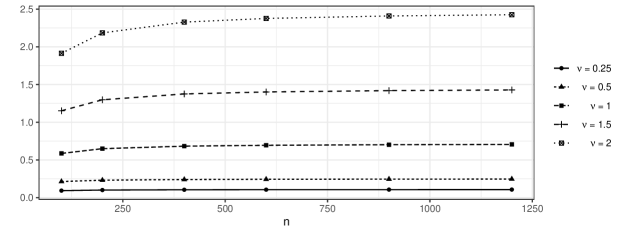
Figure 1: Trend of $\sum_{i=1}^{n}E_{1}(e_{i,1}-e_{i,0})^{2}/E_{1}e_{i,1}^{2}$ for Matérn model when $\chi$ is a regular grid $\chi=\{i\delta:0\leq i\leq n\}$. Parameter $\sigma^{2}$ in Matérn covariogram equals $1.0$ and decay $\phi$ for different $\nu$ are set to make the correlation of two points equals 0.05 when their distance reaches 0.2.

Some additional explanation is also possible from a theoretical viewpoint. Since $P_{0}$ and $P_{1}$ are equivalent, Corollary 3.1 of Stein (1990a) implies that $E_{1}(e_{i,1}-e_{i,0})^{2}/E_{1}e_{i,1}^{2}\to 0$ as $n,i\to\infty$. By stationarity and symmetry of the Matérn model, $e_{i,j}$ is distributed as the error of the least square estimate of $y_{0}:=y(0)$ given observations $y_{(i)}=(y_{1},\ldots,y_{i})^{\top}$. Hence, $e_{i,j}$ can be realized as $y_{0}-E_{j}(y_{0}\,|\,y_{(i)})$. Similarly, $\tilde{e}_{i,j}$ can be realized as $y_{0}-E_{j}(y_{0}\,|\,S_{(i-1)})$. Now consider the infinitely sampled locations $\{i\delta:i\geq 0\}$, and extend the finite sample $Y_{n}:=(y_{0},\ldots,y_{n})^{\top}$ to $Y:=(y_{0},y_{1},\ldots)^{\top}$ with $y_{i}:=y(i\delta)$. The sampled locations of $Y$ form an infinite grid on $[0,\infty)$, and $\delta=1/n$ is determined based on the sample size of $Y_{n}$. Let $e_{\infty,j}$ be the error $y_{0}-E_{j}(y_{0}\,|\,y_{1},\ldots)$ for the infinite sequence $Y$. For $f_{0}$ (resp. $f_{1}$) the spectral density under $P_{0}$ (resp. $P_{1}$), it is easily seen that $f_{0},f_{1}\sim C\sigma_{0}^{2}\phi_{0}^{\nu}u^{-2\nu-1}$ as $u\rightarrow\infty$, and $(f_{1}-f_{0})/f_{0}\asymp u^{-2}$. Therefore, by Theorem 2 of Stein (1999b),

$$\frac{E_{1}(e_{\infty,1}-e_{\infty,0})^{2}}{E_{1}e_{\infty,1}^{2}}=O(\delta^{\min(2\nu+1,4)}\log(\delta^{-1})^{1(\nu=3/2)}))\;.$$ (18)

Intuitively, $e_{i,j}\approx e_{\infty,j}$ for large $i$. It will not be unreasonable to speculate a stronger result where (18) still holds by replacing $e_{\infty,j}$ with $e_{i,j}$ for large $i$, which would imply (17). As indicated on p.138 of Stein (1999a), obtaining the rate of $E_{1}(e_{i,1}-e_{i,0})^{2}/E_{1}e_{i,1}^{2}$ for any bounded domain $\mathcal{D}$ is a highly non-trivial task. The only known results are obtained in Stein (1990b, 1999b) for $\nu=\frac{1}{2},\frac{3}{2},\ldots$, which also imply (17). In fact, we need that $E_{1}e_{i,1}^{2}=E_{1}e_{\infty,1}^{2}(1+\mathcal{O}(i^{-\kappa}))$ for any $\kappa>0$. Hence, the only missing piece in the above heuristics is an estimate of $E_{1}e_{i,0}^{2}/E_{1}e_{\infty,0}^{2}$, which we do not explore further here. Our result is stated as follows.

Theorem 2.

Let $\mathcal{D}=[0,1]$, $\chi=\{i\delta:0\leq i\leq n\}$ and $S_{(i)}=S_{(i)}[n^{\epsilon}]$ for $\epsilon\in(0,1)$. If (17) holds, then (10) also holds. Consequently, (11) holds for the Matérn model ($\nu>0$).

We make a few remarks before presenting a proof. Theorem 2 states that the asymptotic normality of the microergodic parameter $\sigma^{2}\phi^{2\nu}$ still holds under Vecchia’s approximation in a neighborhood of at most size $k=n^{\epsilon}\ll n$ (sample size), where the computation of $\hat{\sigma}^{2}_{n,vecch}$ is much cheaper. This justifies the validity of Vecchia’s approximation for Matérn models from a fixed-domain perspective. The range $n^{\epsilon}$ may not be optimal, and it might be possible to improve to $k=\mathcal{O}(\log n)$. However, we do not pursue this direction here from a theoretical standpoint. A simulation study is provided for the case of $k=\mathcal{O}(\log n)$ in Section IV.

An interesting situation arises with $\nu=1/2$, in which the process reduces to the Ornstein-Uhlenbeck process, and $p(y_{i}\,|\,y_{(i-1)})=p(y_{i}\,|\,y_{i-1})$. Therefore, (11) trivially holds for Vechhia’s approximation with a neighbor of size $k=1=\mathcal{O}(1)$. It is, therefore, natural to enquire whether the asymptotic normality of (11) holds under Vecchia’s approximation within a range $k=\mathcal{O}(1)$. If this is true, computational efforts can be reduced further. Unfortunately, this need not be the case. For $\nu<1/4$ and $k=\mathcal{O}(1)$, $n^{2\nu}(\hat{\sigma}_{n,vecch}^{2}\phi_{1}^{2\nu}-\sigma_{0}^{2}\phi_{0}^{2\nu})$ converges to a non-Gaussian distribution (Bachoc and Lagnoux, 2020). The cases for $\nu\geq 1/4$ remain unresolved.

Now we turn to the proof of Theorem 2. The key to this analysis is the following proposition, which relies on a result on the bound of $e_{\infty,j}-e_{i,j}$, i.e. the difference between the errors of the finite and the infinite least square estimates (Baxter, 1962). The study dates back to the work of Kolmogorov (1941), see also Grenander and Szegö (1958); Ibragimov (1964); Dym and McKean (1970, 1976); Ginovian (1999) for related discussions.

Proposition 1.

Let $\kappa>0$. There exist $C_{0},C_{\kappa}>0$ such that for $\delta<1$ and $j=0,1$,

$$E_{j}e_{\infty,j}^{2}\sim C_{0}\delta^{2\nu},$$ (19)

$$E_{j}(e_{\infty,j}-e_{i,j})^{2}\leq C_{\kappa}\delta^{2\nu}i^{-\kappa}.$$ (20)

Proof.

From the discussion below (17) that $e_{i,j}$ and $e_{\infty,j}$ can be realized as $e_{i,j}=y_{0}-E_{j}(y_{0}\,|\,y_{1},\ldots,y_{i})$ and $e_{\infty,j}=y_{0}-E_{j}(y_{0}\,|\,y_{1},y_{2},\ldots)$, where $y_{i}:=y(i\delta)$ is indexed by nonnegative integers, we know from Stein (1999a, p.77) that the spectral density of $Y$ under $P_{j}$ is

$$\overline{f}^{\delta}_{j}(u)=\frac{1}{\delta}\sum_{\ell=-\infty}^{\infty}f_{j}\left(\frac{u+2\pi\ell}{\delta}\right)\quad\mbox{for }u\in(-\pi,\pi],\quad j=0,1\;,$$

where $f_{j}$ is the spectral density defined by (2) corresponding to $P_{j}$. For $j=0,1$, $f_{j}(u)\sim C\sigma_{0}^{2}\phi_{0}^{2\nu}u^{-2\nu-1}$ as $u\to\infty$. From Stein (1999a, p.80, (17)), we obtain

$$E_{j}e_{\infty,j}^{2}\sim 2\pi C\sigma_{0}^{2}\phi_{0}^{2\nu}\delta^{2\nu}\exp\left(\frac{1}{2\pi}\int_{-\pi}^{\pi}\log\left(\Sigma_{\ell=-\infty}^{\infty}|u+2\pi\ell|^{-2\nu-1}\right)du\right),$$

which implies (19) with

$$C_{0}=2\pi C\sigma_{0}^{2}\phi_{0}^{2\nu}\exp\left(\frac{1}{2\pi}\int_{-\pi}^{\pi}\log\left(\Sigma_{\ell=-\infty}^{\infty}|u+2\pi\ell|^{-2\nu-1}\right)du\right)\;.$$

Turning to (20), we know from Baxter (1962, p.142, (15)) that

$$E_{j}(e_{i,j}-e_{\infty,j})^{2}=E_{j}e_{\infty,j}^{2}\,E_{j}e_{i,j}^{2}\sum_{m=i}^{\infty}|\phi_{m,j}(0)|^{2},$$ (21)

where $\phi_{m,j}(\cdot)$ are the Szegö polynomials associated with the spectral $\overline{f}^{\delta}_{j}$ (see Section 2.1 of Grenander and Szegö, 1958, for background). Note that $E_{j}e_{\infty,j}^{2}\sim C_{0}\delta^{2\nu}$ and $E_{j}e_{i,j}^{2}\leq E_{j}e_{1,j}^{2}\to 0$ as $\delta\to 0$. It will be sufficient to establish

$$\sum_{m=0}^{\infty}m^{\kappa}|\phi_{m,j}(0)|\leq D_{\kappa}\quad\mbox{for some }D_{\kappa}>0,$$ (22)

in which case the identity (21) will imply (20). The key observation of Baxter (1962) (Theorem 2.3) is that (22) holds if the $\kappa^{th}$ moment of the Fourier coefficients associated with $\overline{f}^{\delta}_{j}$ is bounded from above by $D^{\prime}_{\kappa}$ for some $D^{\prime}_{\kappa}>0$, i.e.

$$\sum_{m=0}^{\infty}m^{\kappa}|c_{m,j}|<D_{\kappa}^{\prime},\quad\mbox{where }c_{m,j}:=\frac{1}{2\pi}\int_{-\pi}^{\pi}\overline{f}^{\delta}_{j}(u)e^{-inu}du.$$

A sufficient condition for the latter to hold is that the $\kappa^{th}$ derivative of $\overline{f}^{\delta}_{j}$ is integrable, and $\int_{-\pi}^{\pi}\left|\frac{d^{\kappa}}{du^{\kappa}}\overline{f}^{\delta}_{j}(u)\right|du\leq D^{\prime\prime}_{\kappa}$, for some $D^{\prime\prime}_{\kappa}>0$ which does not depend on $\delta<1$. Breaking the sum of $\overline{f}^{\delta}_{j}$ according to $\ell=0$ and $\ell\neq 0$ produces

$$\int_{-\pi}^{\pi}\left|\frac{d^{\kappa}}{du^{\kappa}}\overline{f}^{\delta}_{j}(u)\right|du\leq A\int_{-\infty}^{\infty}(1+u^{2\nu+1+\kappa})^{-1}du+A^{\prime}\delta^{2\nu}\sum_{\ell\neq 0}l^{-2\nu-1-\kappa}\;,$$ (23)

where $A,A^{\prime}>0$ are numerical constants. Hence, the right hand side of (23) is bounded by $D^{\prime\prime}_{\kappa}=A\int_{-\infty}^{\infty}(1+u^{2\nu+1+\kappa})^{-1}du+A^{\prime}\sum_{\ell\neq 0}l^{-2\nu-1-\kappa}$, which depends only on $\kappa$. ∎

Proof of Theorem 2.

We fix $\kappa=2/\epsilon$, and use $C^{(1)}_{\kappa},C^{(2)}_{\kappa},\ldots$ to denote constants depending only on $\kappa$. Note that $E_{0}e_{i,0}^{2}=E_{0}e_{\infty,0}^{2}+E_{0}(e_{\infty,0}-e_{i,0})^{2}$, since $e_{\infty,0}$ and $e_{\infty,0}-e_{i,0}$ are independent under $P_{0}$. By Proposition 1, we get $E_{0}e_{i,0}^{2}\sim C_{0}\delta^{2\nu}(1+C^{(1)}_{\kappa}i^{-\kappa})$. Similarly, $E_{1}\tilde{e}^{2}_{i,1}=E_{1}e_{\infty,1}^{2}+E_{1}(\tilde{e}_{i,1}-e_{\infty,1})^{2}\sim C_{0}\delta^{2\nu}(1+C^{(2)}_{\kappa}\min(i,n^{\epsilon})^{-\kappa})$, because $\tilde{e}_{i,1}$ is realized as $y_{0}-E_{1}\left(y_{0}\,|\,S_{(i-1)}[k]\right)$ with $k=\min(i,n^{\epsilon})$. Therefore,

$$\sum_{i=1}^{n}\left(\frac{E_{1}\tilde{e}^{2}_{i,1}}{E_{0}e_{i,0}^{2}}-1\right)^{2} \leq\sum_{i\geq n^{\epsilon}}\left(\frac{C^{(3)}_{\kappa}n^{-\epsilon\kappa}}{1+C^{(1)}_{\kappa}i^{-\kappa}}\right)^{2}+\sum_{i=1}^{n}\left(\frac{C^{(4)}_{\kappa}i^{-\kappa}}{1+C^{(1)}_{\kappa}i^{-\kappa}}\right)^{2}$$

$$\leq\frac{C^{(5)}_{\kappa}}{n^{3}}+C^{(6)}_{\kappa}\sum_{i=1}^{n}i^{-2\kappa}\leq C_{\kappa}^{(7)}.$$

Moreover, we have

$$\frac{E_{1}(\tilde{e}_{i,1}-e_{i,0})^{2}}{E_{0}e_{i,0}^{2}}\leq 3\frac{E_{1}(\tilde{e}_{i,1}-e_{\infty,1})^{2}}{E_{0}e_{i,0}^{2}}+3\frac{E_{1}(e_{i,1}-e_{\infty,1})^{2}}{E_{0}e_{i,0}^{2}}+3\frac{E_{1}(e_{i,1}-e_{i,0})^{2}}{E_{1}e_{i,1}^{2}}\frac{E_{1}e_{i,1}^{2}}{E_{0}e_{i,0}^{2}}.$$

By the same argument as above, for the first two terms:

$$\sum_{i=1}^{n}\frac{E_{1}(\tilde{e}_{i,1}-e_{\infty,1})^{2}}{E_{0}e_{i,0}^{2}}<C^{(8)}_{\kappa}\quad\mbox{and}\quad\sum_{i=1}^{n}\frac{E_{1}(e_{i,1}-e_{\infty,1})^{2}}{E_{0}e_{i,0}^{2}}<C^{(9)}_{\kappa}.$$

For the last term,

$$\sum_{i=1}^{n}\frac{E_{1}(e_{i,1}-e_{i,0})^{2}}{E_{1}e_{i,1}^{2}}\frac{E_{1}e_{i,1}^{2}}{E_{0}e_{i,0}^{2}}\leq C^{(10)}_{\kappa}\sum_{i=1}^{n}\frac{E_{1}(e_{i,1}-e_{i,0})^{2}}{E_{1}e_{i,1}^{2}},$$

which converges because of (17). This establishes (10) and, hence, (11) follows. ∎

IV.   Simulations

Based on (12) and (15) provided in Theorem 1, Theorem 2 has proved that

$$c_{n}(\phi_{1},\phi_{0},k)=\frac{1}{\sqrt{n}}\left[\sum_{i=1}^{n}\frac{\tilde{e}_{i,1}^{2}}{E_{1}\tilde{e}_{i,1}^{2}}-\sum_{i=1}^{n}\frac{e_{i,0}^{2}}{E_{0}e_{i,0}^{2}}\right]=o(1)\;$$ (24)

when $k=n^{\epsilon}$ for $\epsilon\in(0,1)$. The equation (24) induces the critical condition (14), resulting in the convergence in law in (11). Looking into the more challenging case $k=\mathcal{O}(\log(n))$, we extend the discussion in Theorem 2 via investigating the behaviour of $c_{n}(\phi_{1},\phi_{0},k)$ in (24) for a sequence of datasets with increasing sample sizes. Our experiments involve two data generation schemes. The first scheme considers the study domains $\mathcal{D}_{1}=[0,1]$ with $n$ observations on the grid $\chi_{1}=\{i/(n-1):0\leq i\leq n-1\}$ and $\mathcal{D}_{2}=[0,1]^{2}$ with $n=n_{s}^{2}$ observations on the grid $\chi_{2}=\{(i/(n_{s}-1),j/(n_{s}-1)):0\leq i,\leq n_{s}-1,0\leq j\leq n_{s}-1\}$. With this scheme, we generate a sequence of datasets with increasing sample size on increasingly finer grids on the study domains. The second scheme generates data on a “disturbed grid”. On $\mathcal{D}_{1}=[0,1]$ with $n$ observations, $\chi_{1}$ comprises locations randomly sampled by $\mbox{N}(i/(n+2),0.15/(n+2))$ for $i=1,\ldots,n$. On $\mathcal{D}_{2}=[0,1]^{2}$ with $n=n_{s}^{2}$ observations, locations in $\chi_{2}$ are generated by $\{N(i/(n_{s}+2),0.15/(n_{s}+2)),N(i/(n_{s}+2),0.15/(n_{s}+2))\}$ for $i,j=1,\ldots,n_{s}$. With this scheme, we first generate simulations with the largest sample size, and then randomly select successively larger subsets from the same dataset to examine the tendency of $c_{n}(\phi_{1},\phi_{0},k)$ with an increasing $n$. The first scheme matches the setup of our proofs in the preceding sections, and the second scheme serves as a more directly informative regime for simulation studies about asymptotics. In practice, estimation using Vecchia’s approximation (4) is complicated by the fixed ordering of locations. Guinness (2018) has provided excellent practical insights into this issue that can considerably improve finite sample behaviour in certain settings. In this study, we test two different orderings of locations, maximin ordering and sorted coordinate ordering. The sorted coordinate ordering orders locations on $\chi_{2}$ first based on the second coordinate and then break ties based on the associated first coordinate. We take $S_{(i)}[k]$ as the at most $k$ nearest neighbors of $y_{i+1}$. In both studies on $\mathcal{D}_{1}$ and $\mathcal{D}_{2}$, we fix $\sigma^{2}=1.0$ and consider $5$ different smoothness values $\nu\in\{0.25,0.5,1.0,1.5,2\}$. We choose different decay parameters $\phi_{0}$ for different $\nu$ so that $K_{\theta}(h)=0.05$ when $h=0.2$ and $0.5$ for the study on $\mathcal{D}_{1}$ and $\mathcal{D}_{2}$, respectively.

For each fixed value of $\theta=\{\sigma^{2},\phi,\nu\}$, we generate $100$ datasets with $Y_{n}$ being the realization from $y(s)\sim GP(0,K_{\theta}(\cdot))$ and calculate $c_{n}(\phi_{1},\phi_{0},k)$ with $k$ being the closest integer to $3\log(n)$, and $\phi_{1}=1.2\phi_{0}$ and $1.1\phi_{0}$ for $\mathcal{D}_{1}$ and $\mathcal{D}_{2}$, respectively. Then, we record the mean and standard deviation of the $100$ values of $c_{n}(\phi_{1},\phi_{0},k)$. We repeat this process for different values of $n$ ranging from $2^{6}=64$ to $2^{12}=4096$ in the study on $\mathcal{D}_{1}$. The study on $\mathcal{D}_{2}$ follows the study on $\mathcal{D}_{1}$ with $n_{s}$ ranging from $9$ to $81$. The code for this simulation study is available on https://github.com/LuZhangstat/vecchia_consistency. Figure 2(a) & 2(b) summarize the study results on $\mathcal{D}_{1}$ under the two data generation schemes. Each figure presents 10 different graphs, one for each value of $\nu$ and each ordering, showing the mean and standard deviation of $c_{n}(\phi_{1},\phi_{0},k)$ for different values of $n$.

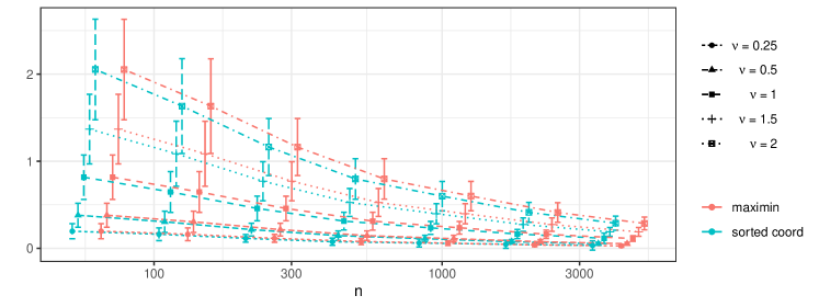
(a) Increasingly finer grids (Data generation scheme 1)

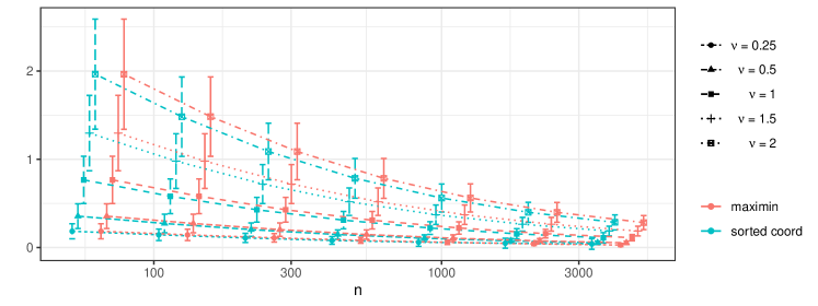
(b) Successively increasing datasets (Data generation scheme 2)

Figure 2: The mean of $c_{n}(\phi_{1},\phi_{0},k)$ of $100$ simulations on $\mathcal{D}_{1}=[0,1]$. The error bars represent one standard deviation. The sample size $n$ take on values in $64,128,256,512,1024,2048$ and $4096$. The graphs in red and blue show the results using maximin ordering and sorted coordinate ordering, respectively.

The value of $c_{n}(\phi_{1},\phi_{0},k)$, as seen in Figure 2, decreases rapidly as the sample size increases, supporting the main conclusion in Theorem 2. We do not observe a strong impact of ordering and data generation scheme on the results. The corresponding graphs for the study on $\mathcal{D}_{2}$ are presented in Figure 3. These graphs also reveal decreasing trends, but with more gentle slopes as compared to Figure 2. The results under the second data generation scheme are slightly better than those under the first scheme. When the smoothness $\nu$ is small, the standard deviation decreases faster with maximin ordering than with sorted coordinate ordering. Meanwhile, the standard deviation doesn’t decrease significantly with the increase of $n$ when $\nu$ is large.

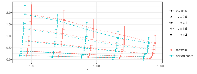
(a) Increasingly finer grids (Data generation scheme 1)

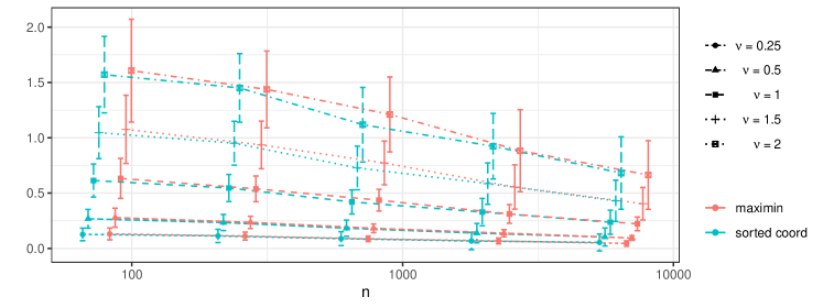
(b) Successively increasing datasets (Data generation scheme 2)

Figure 3: The mean of $c_{n}(\phi_{1},\phi_{0},k)$ of $100$ simulations on $\mathcal{D}_{2}=[0,1]^{2}$. The error bars represent one standard deviation. The sample size $n$ take on values in $81,256,729,2209$ and $6561$. The graphs in red and blue show the results using maximin ordering and sorted coordinate ordering, respectively.

To explore further, we reproduce the study on $\mathcal{D}_{2}$ with $k$ being the closet integer to $\sqrt{n}$, and we illustrate the results in Figure 4. We observe that the standard deviation decreases rapidly as $n$ increases in all cases.

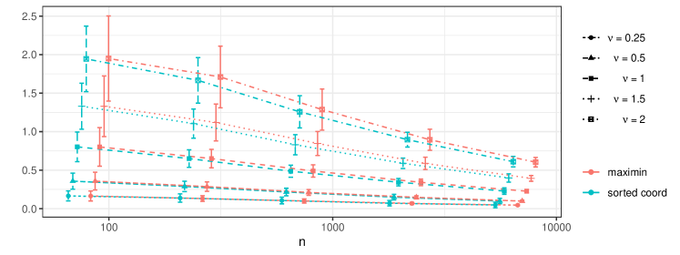
(a) Increasingly finer grids (Data generation scheme 1)

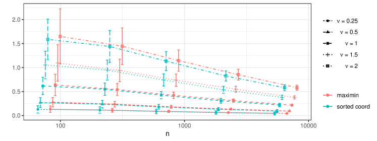
(b) Successively increasing datasets (Data generation scheme 2)

Figure 4: The mean of $c_{n}(\phi_{1},\phi_{0},k)$ of $100$ simulations on $\mathcal{D}_{2}=[0,1]^{2}$. The error bars represent one standard deviation. The sample size $n$ take on values in $81,256,729,2209$ and $6561$. The graphs in red and blue show the results using maximin ordering and sorted coordinate ordering, respectively.

We have also seen, from the proof in Theorem 1, that $c_{n}(k,\phi_{1},\phi_{0})=\sqrt{n}(\hat{\sigma}^{2}_{n,vecch}/\sigma_{1}^{2}-\hat{\sigma}_{0,n}^{2}/\sigma_{0}^{2})$ where $\hat{\sigma}_{0,n}^{2}=\mbox{argmax}_{\sigma^{2}}\{p(y;\phi_{0},\sigma^{2}),\;\sigma^{2}\in\mathbb{R}^{+}\}\;$ is the maximum likelihood estimator from (3) when fixing $\phi_{1}=\phi_{0}$. Hence, $c_{n}(k,\phi_{1},\phi_{0})$ also measures the discrepancy between $\hat{\sigma}^{2}_{n,vecch}/\sigma_{1}^{2}$ and $\hat{\sigma}_{0,n}^{2}/\sigma_{0}^{2}$, and the decreasing trend of $c_{n}(\phi_{0},\phi_{1},k)$ indicates that the inference based on Vecchia’s approximation approaches the inference based on the full likelihood as sample size increases. This phenomenon reveals that Vecchia’s approximation is still efficient when the neighbor size $k$ is substantially smaller than the sample size.

V.   Conclusions and Future work

We have developed insights into inference based on GP likelihood approximations by Vecchia (1988) under fixed domain asymptotics for geostatistical data analysis. We have formally established the sufficient conditions for such approximations to have the same asymptotic efficiency as a full GP likelihood in estimating parameters in Matérn covariance function. The insights obtained here will enhance our understanding of identifiability of process parameters and can also be useful for developing priors for the microergodic parameters in Bayesian modeling. The results derived here will also offer insights into formally establishing posterior consistency of process parameters for a number of Bayesian models that have emerged from (4) (Datta et al., 2016a, b; Katzfuss and Guinness, 2021; Peruzzi et al., 2022).

We anticipate the current manuscript to generate further research in variants of geostatistical models. For example, it is conceivable that these results will lead to asymptotic investigations of covariance-tapered models (see, e.g., Wang et al., 2011) and in adapting some results, such as Theorems 2 and 3 in Kaufman and Shaby (2013) where $\phi$ is estimated, to the approximate likelihoods presented here. Another direction of research can lead to formal developments regarding the inferential consistency of the “nugget” or the variance of measurement error when the spatial process has a discontinuity at $0$ arising white noise (Tang et al., 2021). Finally, there is scope to specifically investigate fixed domain inference for other likelihood approximations that extend or generalize (4) (see, e.g., Katzfuss and Guinness, 2021; Peruzzi et al., 2022).

References

- Abramowitz and Stegun (1965) M. Abramowitz and A. Stegun. Handbook of Mathematical Functions: with Formulas, Graphs, and Mathematical Tables. Dover, 1965.
- Bachoc and Lagnoux (2020) F. Bachoc and A. Lagnoux. Fixed-domain asymptotic properties of maximum composite likelihood estimators for Gaussian processes. J. Statist. Plann. Inference, 209:62–75, 2020.
- Banerjee (2017) Sudipto Banerjee. High-dimensional bayesian geostatistics. Bayesian Analysis, 12:583–614, 2017.
- Baxter (1962) Glen Baxter. An asymptotic result for the finite predictor. Math. Scand., 10:137–144, 1962.
- Datta et al. (2016a) A. Datta, S. Banerjee, A. O. Finley, and A. E. Gelfand. Hierarchical Nearest-Neighbor Gaussian Process Models for Large Geostatistical Datasets. Journal of the American Statistical Association, 111:800–812, 2016a. URL http://dx.doi.org/10.1080/01621459.2015.1044091.
- Datta et al. (2016b) A. Datta, S. Banerjee, A. O. Finley, N. A. S. Hamm, and M. Schaap. Non-separable Dynamic Nearest-Neighbor Gaussian Process Models for Large spatio-temporal Data With an Application to Particulate Matter Analysis. Annals of Applied Statistics, 10:1286–1316, 2016b. URL http://dx.doi.org/10.1214/16-AOAS931.
- Du et al. (2009) J. Du, H. Zhang, and V. S. Mandrekar. Fixed-domain asymptotic properties of tapered maximum likelihood estimators. The Annals of Statistics, 37(6A):3330–3361, 2009.
- Dym and McKean (1970) H. Dym and H. P. McKean. Extrapolation and interpolation of stationary Gaussian processes. Ann. Math. Statist., 41:1817–1844, 1970.
- Dym and McKean (1976) H. Dym and H. P. McKean. Gaussian processes, function theory, and the inverse spectral problem. Academic Press [Harcourt Brace Jovanovich, Publishers], New York-London, 1976. Probability and Mathematical Statistics, Vol. 31.
- Eidsvik et al. (2014) Jo Eidsvik, Benjamin A. Shaby, Brian J. Reich, Matthew Wheeler, and Jarad Niemi. Estimation and prediction in spatial models with block composite likelihoods. Journal of Computational and Graphical Statistics, 23(2):295–315, 2014. doi: 10.1080/10618600.2012.760460. URL https://doi.org/10.1080/10618600.2012.760460.
- Finley et al. (2019) Andrew O Finley, Abhirup Datta, Bruce C Cook, Douglas C Morton, Hans E Andersen, and Sudipto Banerjee. Efficient algorithms for Bayesian Nearest Neighbor Gaussian Processes. Journal of Computational and Graphical Statistics, 28(2):401–414, 2019.
- Ginovian (1999) M. S. Ginovian. Asymptotic behavior of the prediction error for stationary random sequences. Izv. Nats. Akad. Nauk Armenii Mat., 34(1):18–36 (2000), 1999.
- Grenander and Szegö (1958) Ulf Grenander and Gabor Szegö. Toeplitz forms and their applications. California Monographs in Mathematical Sciences. University of California Press, Berkeley-Los Angeles, 1958.
- Guinness (2018) Joseph Guinness. Permutation and grouping methods for sharpening Gaussian process approximations. Technometrics, 60(4):415–429, 2018.
- Heaton et al. (2019) Matthew J Heaton, Abhirup Datta, Andrew O Finley, Reinhard Furrer, Joseph Guinness, Rajarshi Guhaniyogi, Florian Gerber, Robert B Gramacy, Dorit Hammerling, Matthias Katzfuss, et al. A case study competition among methods for analyzing large spatial data. Journal of Agricultural, Biological and Environmental Statistics, 24(3):398–425, 2019.
- Ibragimov (1964) I. A. Ibragimov. On the asymptotic behavior of the prediction error. Theory of Probability & Its Applications, 9(4):627–634, 1964.
- Ibragimov and Rozanov (1978) Ildar Abdullovich Ibragimov and Y. A. Rozanov. Gaussian random processes, volume 9 of Applications of Mathematics. Springer-Verlag, New York-Berlin, 1978. Translated from the Russian by A. B. Aries.
- Katzfuss and Guinness (2021) Matthias Katzfuss and Joseph Guinness. A general framework for vecchia approximations of gaussian processes. Statist. Sci., 36(1):124–141, 02 2021. doi: 10.1214/19-STS755. URL https://doi.org/10.1214/19-STS755.
- Katzfuss et al. (2020) Matthias Katzfuss, Joseph Guinness, Wenlong Gong, and Daniel Zilber. Vecchia approximations of Gaussian-process predictions. Journal of Agricultural, Biological and Environmental Statistics, 25(3):383–414, 2020.
- Kaufman and Shaby (2013) C. G. Kaufman and B. A. Shaby. The role of the range parameter for estimation and prediction in geostatistics. Biometrika, 100(2):473–484, 2013.
- Kolmogorov (1941) A. Kolmogorov. Interpolation und Extrapolation von stationären zufälligen Folgen. Bull. Acad. Sci. URSS Sér. Math. [Izvestia Akad. Nauk. SSSR], 5:3–14, 1941.
- Matérn (1986) B. Matérn. Spatial Variation. Springer-Verlag, 1986.
- Peruzzi et al. (2022) Michele Peruzzi, Sudipto Banerjee, and Andrew O. Finley. Highly scalable bayesian geostatistical modeling via meshed gaussian processes on partitioned domains. Journal of the American Statistical Association, 117(538):969–982, 2022. doi: 10.1080/01621459.2020.1833889. URL https://doi.org/10.1080/01621459.2020.1833889.
- Shiryaev (1996) A. N. Shiryaev. Probability, volume 95 of Graduate Texts in Mathematics. Springer-Verlag, New York, second edition, 1996.
- Stein (1999a) M. L. Stein. Interpolation of Spatial Data: Some Theory for Kriging. Springer-Verlag, 1999a.
- Stein (1990a) Michael L. Stein. Uniform asymptotic optimality of linear predictions of a random field using an incorrect second-order structure. Ann. Statist., 18(2):850–872, 1990a.
- Stein (1990b) Michael L. Stein. Bounds on the efficiency of linear predictions using an incorrect covariance function. Ann. Statist., 18(3):1116–1138, 1990b.
- Stein (1999b) Michael L. Stein. Predicting random fields with increasing dense observations. Ann. Appl. Probab., 9(1):242–273, 1999b.
- Stein et al. (2004) Michael L Stein, Zhiyi Chi, and Leah J Welty. Approximating likelihoods for large spatial data sets. Journal of the Royal Statistical Society: Series B (Statistical Methodology), 66(2):275–296, 2004.
- Sun et al. (2012) Ying Sun, Bo Li, and Marc G Genton. Geostatistics for large datasets. In Advances and challenges in space-time modelling of natural events, pages 55–77. Springer, 2012.
- Tang et al. (2021) Wenpin Tang, Lu Zhang, and Sudipto Banerjee. On identifiability and consistency of the nugget in Gaussian spatial process models. J. R. Stat. Soc. Ser. B. Stat. Methodol., 83(5):1044–1070, 2021.
- Vecchia (1988) A. V. Vecchia. Estimation and model identification for continuous spatial processes. Journal of the Royal Statistical society, Series B, 50:297–312, 1988.
- Wang et al. (2011) Daqing Wang, Wei-Liem Loh, et al. On fixed-domain asymptotics and covariance tapering in gaussian random field models. Electronic Journal of Statistics, 5:238–269, 2011.
- Zhang (2004) Hao Zhang. Inconsistent estimation and asymptotically equal interpolations in model-based geostatistics. Journal of the American Statistical Association, 99(465):250–261, 2004.
- Zhang (2012) Hao Zhang. Asymptotics and computation for spatial statistics. In Advances and Challenges in Space-time Modelling of Natural Events, pages 239–252. Springer, 2012.
- Zhang and Zimmerman (2005) Hao Zhang and Dale L Zimmerman. Towards reconciling two asymptotic frameworks in spatial statistics. Biometrika, 92(4):921–936, 2005.
- Zhang et al. (2019) Lu Zhang, Abhirup Datta, and Sudipto Banerjee. Practical bayesian modeling and inference for massive spatial datasets on modest computing environments. Statistical Analysis and Data Mining: The ASA Data Science Journal, 12(3):197–209, 2019. doi: 10.1002/sam.11413. URL https://doi.org/10.1002/sam.11413.