Electronic spectrum of Kekulé patterned graphene considering second neighbor-interactions

Abstract

The effects of second-neighbor interactions in Kekulé patterned graphene electronic properties are studied starting from a tight-binding Hamiltonian. Thereafter, a low-energy effective Hamiltonian is obtained by projecting the high energy bands at the $\Gamma$ point into the subspace defined by the Kekulé wave vector. The spectrum of the low energy Hamiltonian is in excellent agreement with the one obtained from a numerical diagonalization of the full tight-binding Hamiltonian. The main effect of the second-neighbour interaction is that a set of bands gains an effective mass and a shift in energy, thus lifting the degeneracy of the conduction bands at the Dirac point. This band structure is akin to a “spin-one Dirac cone”, a result expected for honeycomb lattices with a distinction between one third of the atoms in one sublattice. Finally, we present a study of Kekulé patterned graphene nanoribbons. This shows that the previous effects are enhanced as the width decreases. Moreover, edge states become dispersive, as expected due to second neighbors interaction, but here the Kek-Y bond texture results in an hybridization of both edge states. The present study shows the importance of second neighbors in realistic models of Kekulé patterned graphene, specially at surfaces.

I Intoduction

The space-modulation of two-dimensional materials has opened avenues for new exciting physical phenomena and applications MOGERA2020470 ; Wu_2020 ; NaumisReview ; Chen2019 ; Yankowitz2018 ; Ni2015 ; Taboada2017 ; Ohta2012 ; Bistritzer ; Zheng2016 . Several mechanisms allow to perform such modulations, these include interactions with substrateszhou2007substrate as in moire patternsponomarenko2013cloning , strainvozmediano2010gauge ; amorim2016novel ; naumis2017electronic , adatomsBianchi2010 ; Kaasbjerg2019 , magnetic fieldsnovoselov2004electric ; jiang2007infrared ; guinea2006electronic , and time dependent electromagnetic fieldseckardt2015high ; LaserGap ; FloquetTop .

Among such modulated systems, in graphene it has been experimentally observed that vacancies in a Cu substrate induce a spatial frequency modulation with the size of an hexagonal ring of carbon atoms Gutierrez2016 . This modulated system is known as kekulé-distorted graphene Gutierrez2016 ; Gamayun ; Elias_2019 ; Wu2020 ; Tijerina_2019 ; Hoi_2019 ; Penglin_2019 . As an example of its interest and importance, such kekulé distortion has been proposed as a possible mechanism behind superconductivity in magic-angle twisted bilayer graphene Bitan_2010 ; Hoi_2019 . Also, strain in kekulé distorted graphene can be used to perform valleytronics Elias_2019 , a feature that recently has been experimentally confirmed Daejin . Multiflavor Dirac fermions were predicted to emerge in kekulé graphene bilayers Tijerina_2019 , and it is even possible to produce such modulation in non-atomic systems, as with mechanical waves in solids Mendez2020 and acoustical lattices Penglin_2019 . Kekulé modulations are also reacheable via photonic Photonic_2019 , polaronic Cerda2013 and atomic systems Atomic_2019 .

Gamayun et. al demostrated the absence of a gap for a Kek-Y distortion and deduced the low energy Hamiltonian for Kekulé distortions by using a first-neighbor tight-binding Hamiltonian Gamayun . They show how the two Dirac cones merge at the center of the Brillouin zone, producing either a gap (Kek-O) or the superposition of two cones with different Fermi velocities (Kek-Y)Gamayun .

Several works have been made using such first-neighbor tight-binding Hamiltonian, for example to study uniaxial strainElias_2019 ; Eom2020Direct and the electronic transport properties KuboKek ; Elias2020 ; Barrier-Kek ; kek-device .

However, its is known that second-neighbors interactions in graphene are very important Castro_Neto ; Botello . They are fundamental to explain the electronic properties at graphene surface as in graphene nanoribbons Castro_Neto . This leads to the natural question of what are the effects of second neighbors interactions in a Kekulké patterns. Although Density Functional Calculations already contains such effects, due to the involved energies and the low resolution of the mesh calculations near the Dirac cones, its is difficult to assert a detailed picture of the energy dispersion. In that sense, a tight-binding calculation can be very useful. Here we tackle this question by producing a low-energy Hamiltonian for a Kekulé patterned graphene which includes second-neighbor interactions. The resulting model is validated through a comparison with the numerical calculations.

The paper is organized as follows. In Sec. First and second neighbor Kekulé-Y graphene Hamiltonian we introduce the Hamiltonian for a honeycomb lattice with a Kek-Y distortion up to next-nearest neighbors, and in Sec. Low-Energy Hamiltonian we calculate an effective four band low-energy Hamiltonian, finally in II we present our conclusions and remarks.

First and second neighbor Kekulé-Y graphene Hamiltonian

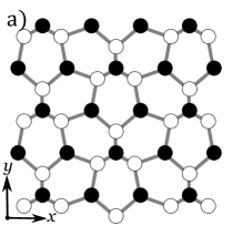
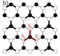
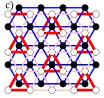
Figure 1: Kek-Y distorted graphene lattice. The A and B sublattices are denoted by the black and white circles respectively. a) Deformed lattice, not in scale for illustration purposes. b) Nearest neighbors hoppings. The bold black lines indicate a stronger bond than the gray ones. c) Next-nearest neighbors interactions scheme. They form two independent triangular lattices for each sublattice, here shown in blue for the one corresponding to the A sublattice. These A-A bonds remain unaltered by the Kek-Y pattern. For the B sublattice, a B-B bond texture is induced in such a way that the bonds near the Y deformation (bold red lines) are stronger than the others (pink lines).

We can consider the Kek-Y bond modulation as a periodic strain which reduces the distance between one third of the atoms in one sublattice with its three nearest neighbors as shown in Fig. 1a. Thus the hopping integral gets modified by the change in the interatomic distances accordingly with strain theory naumis2017electronic . However, this would also mean a change in the next-nearest neighbors hoppings. In Fig. 1c we illustrate this point, by showing in red (pink) the stronger (weaker) bonds for the B sublattice. In blue we show the hoppings between the A sublattice atoms, which remain unaltered.

Assuming the Gruneissen parameter to be equal for both first and second neighbors we can consider that the bond changes with the same proportionality. Thus the Hamiltonian for graphene with Kek-Y distortion considering hopping up to next-nearest neighbors is,

$$H=-\sum_{\bm{r}}\sum_{j=1}^{3}t^{(0)}_{\bm{r}}a_{\bm{r}}^{\dagger}b_{\bm{r+\delta_{j}}}+h.c.+\sum_{\bm{r}}\sum_{m\neq n}t_{2}a_{\bm{r}}^{\dagger}a_{\bm{r+\delta_{m}-\delta_{n}}}+\sum_{\bm{r}}\sum_{m\neq n}t^{(2)}_{\bm{r}}b_{\bm{r}+\delta_{m}}^{\dagger}b_{\bm{r+\delta_{n}}},$$ (1)

where $\bm{r}$ is the position vector that runs over the atomic positions of sites in sublattice A and its given by $\bm{r}=n_{1}\bm{a}_{1}+n_{2}\bm{a}_{2}$ where $n_{1}$, $n_{2}$ are integers, $\bm{a}_{1}=a\left(-\frac{\sqrt{3}}{2},\frac{3}{2}\right)$, $\bm{a}_{2}=a\left(\frac{\sqrt{3}}{2},\frac{3}{2}\right)$ are the lattice vectors and $a$ is the distance between carbon atoms $1.42$ Å. The vectors $\delta_{1}=a\left(\frac{\sqrt{3}}{2},-\frac{1}{2}\right)$, $\delta_{2}=a\left(-\frac{\sqrt{3}}{2},-\frac{1}{2}\right)$ and $\delta_{3}=a\left(0,1\right)$ go from a site in the A sublattice towards its three nearest neighbors in the B sublattice as shown in Fig. 1. The space dependent hopping parameters $t_{\bm{r}}^{(0)}$ and $t_{\bm{r}}^{(2)}$ between nearest neighbors and next-nearest neighbors respectively, are periodically modulated as

$$t_{\bm{r}}^{(0)}/t_{0}=t_{\bm{r}}^{(2)}/t_{2}=1+2\Delta\text{cos}(\bm{G}\cdot\bm{r}),$$ (2)

here $t_{0}=2.8$ eV is the hopping parameter for first neighbors in pristine graphene, and $t_{2}$ for second neighbors which will be taken as $t_{2}=0.1t_{0}$ unless otherwise indicated. $\Delta$ is the Kekulé coupling amplitude and $\bm{G}=\frac{4\pi}{9}\sqrt{3}(1,0)$ is the Kekulé wave vector. The Fourier transform of our tight-binding Hamiltonian is then,

$$\begin{split}H(\bm{k})=&-\epsilon(\bm{k})a^{\dagger}_{\bm{k}}b_{\bm{k}}-\Delta\epsilon(\bm{k+G})a_{\bm{k+G}}^{\dagger}b_{\bm{k}}-\Delta\epsilon(\bm{k-G})a_{\bm{k-G}}^{\dagger}b_{\bm{k}}+h.c.\\ &+f(\bm{k})a_{\bm{k}}^{\dagger}a_{\bm{k}}+f(\bm{k})b_{\bm{k}}^{\dagger}b_{\bm{k}}+\Delta f^{+}(\bm{k})b_{\bm{k+G}}^{\dagger}b_{\bm{k}}+\Delta f^{-}(\bm{k})b_{\bm{k-G}}^{\dagger}b_{\bm{k}},\end{split}$$ (3)

where

$$\epsilon(k)=t_{0}\sum_{j=1}^{3}e^{i\bm{k\cdot\delta_{j}}},$$ (4a)

$$f(k)=t_{2}\sum_{m\neq n}e^{i\bm{k\cdot(\delta_{m}-\delta_{n})}},$$ (4b)

$$f^{\pm}(k)=t_{2}\sum_{m\neq n}e^{i\bm{k\cdot(\delta_{m}-\delta_{n})}}e^{\mp i\bm{G\cdot\delta_{n}}},$$ (4c)

here $\epsilon(\bm{k})$ and $f(\bm{k})$ are the dispersion relations for a honeycomb and a triangular lattice respectively. Some properties of $f^{\pm}(\bm{k})$ are:

$$f^{\pm^{*}}(\bm{k}\pm\bm{G})=f^{\mp}(\bm{k}\mp\bm{G}),\quad f^{\mp^{*}}(\bm{k}\pm\bm{G})=f^{\pm}(\bm{k}).$$ (5)

By defining the column vector $c_{\bm{k}}=(a_{\bm{k}},b_{\bm{k}},a_{\bm{k+G}},b_{\bm{k+G}},a_{\bm{k-G}},b_{\bm{k-G}})$ we can rewrite the Hamiltonian as a 6 x 6 matrix:

$$H(\bm{k})=c_{\bm{k}}^{\dagger}\begin{pmatrix}H_{\Gamma}&T\\ T^{\dagger}&H_{G}\end{pmatrix}c_{\bm{k}},$$ (6a)

made from the original $$\Gamma$$ point graphene Hamiltonian,

$$H_{\Gamma}=\begin{pmatrix}f(\bm{k})&-\epsilon(\bm{k})\\ -\epsilon(\bm{k})&f(\bm{k})\\ \end{pmatrix},$$ (6b)

the $$\bm{G} \bm{-G}$$ and points Hamiltonian,

$$H_{G}=\begin{pmatrix}f(\bm{k+G})&-\epsilon(\bm{k+G})&0&-\Delta\epsilon(\bm{k-G})\\ -\epsilon^{*}(\bm{k+G})&f(\bm{k+G})&-\Delta\epsilon^{*}(\bm{k+G})&\Delta f^{-}(\bm{k-G})\\ 0&-\Delta\epsilon(\bm{k+G})&f(\bm{k-G})&-\epsilon(\bm{k-G})\\ -\Delta\epsilon^{*}(\bm{k-G})&\Delta f^{+}(\bm{k+G})&-\epsilon^{*}(\bm{k-G})&f(\bm{k-G})\\ \end{pmatrix},$$ (6c)

and the interaction between them,

$$T=\begin{pmatrix}0&-\Delta\epsilon(\bm{k+G})&0&-\Delta\epsilon(\bm{k-G})\\ -\Delta\epsilon^{*}(\bm{k})&\Delta f^{-}(\bm{k+G})&-\Delta\epsilon^{*}(\bm{k})&\Delta f^{+}(\bm{k-G})\end{pmatrix}.$$ (6d)

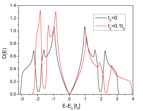
Figure 2: Comparison of the DOS for Kekulé patterned graphene with and without the second-neighbor interaction, where the zero energy corresponds to the Fermi energy. Notice the electron-hole asymmetry which is specially clear for the band widths.

In Fig. 2 we present the density of states (DOS) obtained from a numerical diagonalization of Eq. (6a). As expected, the main effect is the breaking of the electron-hole symmetry reflected in changes of the band widths. Also, around the Fermi energy there are changes that we explore in the following section, as we will develop a low-energy approximation and compare it with the numerical diagonalization of the Hamiltonian given in (6a).

Low-Energy Hamiltonian

Let us now build a low energy Hamiltonian starting with the full $6\times 6$ Hamiltonian given by Eq. (6a). Since we are interested in the low energy bands, we expand up to first order in $\bm{k}$ the functions that appear in Eq. (6a). We obtain the following results,

$$\epsilon(\bm{k})\approx 3t_{0},\quad\epsilon(\bm{k\pm G})\approx\frac{3}{2}t_{0}(\mp k_{x}+ik_{y}),$$ (7a)

$$f(\bm{k})\approx 6t_{2},\quad f(\bm{k\pm G})\approx-3t_{2},$$ (7b)

$$f^{\pm}(\bm{k\pm G})\approx 0,\quad f^{\pm}(\bm{k\mp G})\approx\frac{9}{2}t_{2}(\pm k_{x}+ik_{y}),\quad f^{\pm}(\bm{k})\approx\frac{9}{2}t_{2}(\mp k_{x}-ik_{y}).$$ (7c)

Using the previous approximations, the linearized components of the Hamiltonian Eq. (6a) are given by,

$$H_{\Gamma}\approx\begin{pmatrix}6t_{2}&-3t_{0}\\ -3t_{0}&6t_{2}\\ \end{pmatrix},$$ (8a)

$$H_{G}\approx\begin{pmatrix}-3t_{2}&v_{F}\hbar(k_{x}-ik_{y})&0&-\Delta v_{F}\hbar(k_{x}+ik_{y})\\ v_{F}\hbar(k_{x}+ik_{y})&-3t_{2}&\Delta v_{F}\hbar(k_{x}+ik_{y})&0\\ \ \par 0&\Delta v_{F}\hbar(k_{x}-ik_{y})&-3t_{2}&-v_{F}\hbar(k_{x}+ik_{y})\\ -\Delta v_{F}\hbar(k_{x}-ik_{y}))&0&-v_{F}\hbar(k_{x}-ik_{y})&-3t2\\ \end{pmatrix},$$ (8b)

$$T\approx\begin{pmatrix}0&\Delta v_{F}\hbar(k_{x}-ik_{y})&0&-\Delta v_{F}\hbar(k_{x}+ik_{y})\\ -3\Delta t_{0}&-\Delta v_{2}\hbar(k_{x}-ik_{y})&-3\Delta t_{0}&\Delta v_{2}\hbar(k_{x}+ik_{y})\end{pmatrix},$$ (8c)

where we defined two velocities, one is the usual Fermi velocity in pristine graphene,

$$v_{F}=\frac{3at_{0}}{2\hbar}$$ (9)

and the other is due to second neighbors,

$$v_{2}=\frac{9at_{2}}{2\hbar}=3\left(\frac{t_{2}}{t_{0}}\right)v_{F}.$$ (10)

As we are interested in the spectrum at low energies, the relevant part is the one associated with the valleys $\bm{K}$ and $\bm{K^{\prime}}$ which corresponds to the block matrix $H_{G}$, and then we can add the effects from higher energy bands in the $\bm{\Gamma}$ point as a perturbation. We have verified that this is an essential step in order to recover the spectrum obtained from a direct diagonalization. We can obtain the effective Hamiltonian by projecting $H_{\Gamma}$ into the subspace of $H_{G}$. To do this, consider the Schrodinger equation applied to Eq. (6a),

$$H_{\Gamma}\Psi_{\bm{\Gamma}}+T\Psi_{\bm{G}}=E\Psi_{\Gamma}$$ (11)

and

$$T^{\dagger}\Psi_{\bm{\Gamma}}+H_{\bm{G}}\Psi_{\bm{G}}=E\Psi_{\bm{G}}$$ (12)

where $\Psi_{\Gamma}$ and $\Psi_{\bm{G}}$ are the components of the solution $\Psi=(\Psi_{\Gamma},\Psi_{\bm{G}})$ on each subspace.

From the first equation we can obtain $\Psi_{\Gamma}$ and use it on the second to obtain an effective Hamiltonian for the $\Psi_{\bm{G}}$ component resulting in an effective Hamiltonian,

$$H_{Eff}=H_{G}+T^{\dagger}(E\mathds{1}-H_{\Gamma})^{-1}T$$ (13)

This Hamiltonian is exact but needs a self-consistent procedure to find $E$. However, if we expand the term $(E\mathds{1}-H_{\Gamma})^{-1}$ and keep the first order term. we can make the approximation $E\approx E_{0}=-3t_{2}$ which is the original energy dispersion in the $\Gamma$ point. Now we write the Dirac-like equation for this system,

$$\mathcal{H}\begin{pmatrix}\Psi_{\bm{K}^{\prime}}\\ \Psi_{\bm{K}}\end{pmatrix}=E\begin{pmatrix}\Psi_{\bm{K}^{\prime}}\\ \Psi_{\bm{K}}\end{pmatrix},$$ (14a)

$$\Psi_{\bm{K}^{\prime}}=\begin{pmatrix}-\psi_{B,\bm{K}^{\prime}}\\ \psi_{A,\bm{K}^{\prime}}\end{pmatrix},\quad\Psi_{\bm{K}}=\begin{pmatrix}\psi_{A,\bm{K}}\\ \psi_{K,\bm{K}}\end{pmatrix},$$ (14b)

where the explicit form of the low-energy Hamiltonian is finally given by,

$$\mathcal{H}=\begin{pmatrix}E_{0}&v_{F}(1-\Delta^{2})(p_{x}-ip_{y})&v_{F}\Delta(1-\Delta)(p_{x}-ip_{y})&0\\ v_{F}(1-\Delta^{2})(p_{x}+ip_{y})&E_{0}+\mu&\mu&v_{F}\Delta(1-\Delta)(p_{x}-ip_{y})\\ v_{F}\Delta(1-\Delta^{2})(p_{x}+ip_{y})&\mu&E_{0}+\mu&v_{F}(1-\Delta^{2})(p_{x}-ip_{y})\\ 0&v_{F}\Delta(1-\Delta^{2})(p_{x}+ip_{y})&v_{F}(1-\Delta^{2})(p_{x}+ip_{y})&E_{0}\end{pmatrix},$$

which can be compactly written as,

$$\begin{split}\mathcal{H}=&E_{0}\bm{\sigma}_{0}\otimes\bm{\tau}_{0}+v_{f}(1-\Delta^{2})(\bm{p}\cdot\bm{\sigma})\otimes\bm{\tau}_{0}+v_{f}\Delta(1-\Delta)\bm{\sigma}_{0}\otimes(\bm{p}\cdot\bm{\tau})\\ &+\frac{\mu}{2}(\bm{\sigma}_{0}\otimes\bm{\tau}_{0}+\bm{\sigma}_{x}\otimes\bm{\tau}_{x}+\bm{\sigma}_{y}\otimes\bm{\tau}_{y}-\bm{\sigma}_{z}\otimes\bm{\tau}_{z}),\end{split}$$ (14c)

with $\mu$ defined as,

$$\mu=\frac{9\Delta^{2}t_{0}^{2}t_{2}}{t_{0}^{2}-9t_{2}^{2}}.$$ (15)

The four low-energy bands are

$$E_{D}^{\pm}=E_{0}\pm v_{D}|\bm{p}|,$$ (16a)

$$E_{M}^{\pm}=E_{0}+\mu\pm\sqrt{v_{M}^{2}\bm{p}^{2}+\mu^{2}},$$ (16b)

were we defined $v_{D}=v_{F}(1-\Delta)$ and $v_{M}=v_{F}(1-\Delta)(1+2\Delta)$.

Therefore, there is a mix of two-flavor Fermion gases. One with and effective Dirac Hamiltonian,

$$H_{D}=E_{0}\bm{\sigma}_{0}+v_{D}\bm{p}\cdot\bm{\sigma},$$ (17)

and the other,

$$H_{M}=(E_{0}+\mu)\bm{\sigma}_{0}+v_{M}\bm{p}\cdot\bm{\sigma}+\mu\bm{\sigma}_{z}.$$ (18)

In Fig. 3 we compare our results from Eq. (16b) with the numerical diagonalization of the tight-binding Hamiltonian given by Eq. (6a). First we notice an excellent agreement within this regime. Without second neighbors interaction, the Kek-Y bond texture couples both valleys in the $\Gamma$ point, resulting in two concentric cones with different velocities Gamayun . Turning on the interaction gives rise to two main effects, a set of bands gains an effective mass and a shift in energy. This last effect results in a particle-hole symmetry breaking, lifting the degeneracy of the conduction bands at the Dirac point, therefore only three bands intersect. This structure is akin to a “spin-one Dirac cone”, expected for a honeycomb lattices with a distinction between one third of the atoms in one sublattice single_valley ; pseudospin_one . We can see that the effect of adding next-nearest-neighbors interaction is equivalent to that of an on-site potential $\mu$ on the atom at which the Y deformation is centered Gamayun .

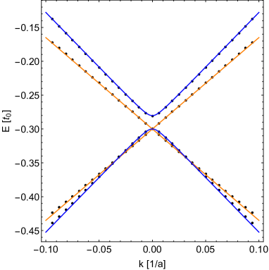
Figure 3: Low-energy dispersion around the $\Gamma$ point with $\Delta=0.1$ and $t_{2}/t_{0}=0.1$. The solid lines indicate our analytic results for both the conic (orange) and the bands with an effective mass (blue). The numerical tight-binding calculations obtained by a direct diagonalization of the Hamiltonian are represented by the dots.

From Eq. (16b) we can easily calculate the density of states per unit cell. Considering spin degeneracy, it is given by,

$$D(E)=\frac{A}{\pi\hbar^{2}}\left[\frac{|E-E_{0}|}{v_{D}^{2}}+\frac{E-(E_{0}+\mu)}{v_{M}^{2}}\Theta(E-E_{0}-2\mu)+\frac{(E_{0}+\mu)-E}{v_{M}^{2}}\Theta(E_{0}-E)\right],$$ (19)

where $A=9\sqrt{3}a^{2}/2$ is the unit cell area and $\Theta(E)$ is the Heaviside function. Although the density of states retains its linear behavior around the Dirac point, the massive bands produce a discontinuity shown in Fig. 4.

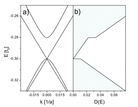
Figure 4: a) A zoom of the energy dispersion around the Fermi energy of Kekulé patterned graphene including up to second-neighbor interactions obtained from the low-energy approximation. b) The corresponding density of states showing how the cone with an effective mass produces two jumps in the DOS.

Second neighbors hoppings are particularly important for graphene nanoribbons (GNR). We calculated numerically the band structure for zigzag edged GNR. In Fig. 5 our results are shown for different values of $t_{2}$ and width $W$. Due to the change in the periodicity produced by the Kekulé texture, the unit cell size $a_{z}$ is three times bigger, thus $a_{z}=3\sqrt{3}a$. We can see that edge states become dispersive, which is a well known effect of second neighbors interaction Castro_Neto , however the combination with the Kek-Y bond texture results in an hybridization of both edge states. The velocity induced in the edge states may indirectly close the small gap predicted for Kek-Y zigzag GNR Elias2020 .

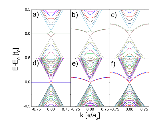
Figure 5: Dispersion for zigzag graphene nanoribbons with Kekulé-Y bond texture and hoppings up to next nearest neighbors. The amplitude of the bond texture is $\Delta=0.1$ for all figures. a), b) and c) show the dispersion with $t_{2}/t_{0}=0,0.1$ and $0.2$ respectively for a ribbon with $W=4.54$ nm, analogously d), e) and f) for a ribbon with $W=13.06$ nm.

II Conclusions

The effects of second-neighbor interactions in Kekulé patterned graphene were studied starting from a tight-binding Hamiltonian. From there, a low-energy effective Hamiltonian was derived using a projection technique. This Hamiltonian was validated thorough a comparison with a numerical calculation obtained from the diagonalization of the full tight-binding Hamiltonian. We found that beyond the expected electron-hole symmetry breaking, the main effect of the second-neighbor interaction is that in one of the Dirac cones, the electron becomes massive when compared with the calculation made considering only first-neighbour interaction. As a result, the density of states near the Fermi energy contains a jump in the otherwise linear behavior. Finally, we considered the effects of second-neighbor interactions in Kekulé patterned graphene nanoribbons, as it is known that such effects are essential to reproduce a minimally realistic behavior at the edges. As expected, the same mass effect is seen in the nanoribbons and in fact is amplified as the width is decreased.

Thus, we expect that such second-neighbor effects to be important in the electronic and optical properties of Kekulé bond textures.

We thank UNAM DGAPA project IN102620 and CONACYT project 1564464. E. Andrade thanks an schoolarship from CONACyT.

References

- [1] Umesha Mogera and Giridhar U. Kulkarni. A new twist in graphene research: Twisted graphene. Carbon, 156:470 – 487, 2020.
- [2] Di Wu, Yi Pan, and Tai Min. Twistronics in graphene, from transfer assembly to epitaxy. Applied Sciences, 10(14):4690, Jul 2020.
- [3] Gerardo G. Naumis, Salvador Barraza-Lopez, Maurice Oliva-Leyva, and Humberto Terrones. Electronic and optical properties of strained graphene and other strained 2D materials: a review. Reports on Progress in Physics, 80:096501, Sep 2017.
- [4] Guorui Chen, Lili Jiang, Shuang Wu, Bosai Lyu, Hongyuan Li, Bheema Lingam Chittari, Kenji Watanabe, Takashi Taniguchi, Zhiwen Shi, Jeil Jung, Yuanbo Zhang, and Feng Wang. Evidence of a gate-tunable mott insulator in a trilayer graphene moiré superlattice. Nature Physics, 15(3):237–241, Mar 2019.
- [5] Matthew Yankowitz, Jeil Jung, Evan Laksono, Nicolas Leconte, Bheema L. Chittari, K. Watanabe, T. Taniguchi, Shaffique Adam, David Graf, and Cory R. Dean. Dynamic band-structure tuning of graphene moiré superlattices with pressure. Nature, 557(7705):404–408, May 2018.
- [6] G. X. Ni, H. Wang, J. S. Wu, Z. Fei, M. D. Goldflam, F. Keilmann, B. Özyilmaz, A. H. Castro Neto, X. M. Xie, M. M. Fogler, and D. N. Basov. Plasmons in graphene moiré superlattices. Nature Materials, 14(12):1217–1222, Dec 2015.
- [7] Pedro Roman-Taboada and Gerardo G. Naumis. Topological edge states on time-periodically strained armchair graphene nanoribbons. Phys. Rev. B, 96:155435, Oct 2017.
- [8] Taisuke Ohta, Jeremy T. Robinson, Peter J. Feibelman, Aaron Bostwick, Eli Rotenberg, and Thomas E. Beechem. Evidence for interlayer coupling and moiré periodic potentials in twisted bilayer graphene. Phys. Rev. Lett., 109:186807, Nov 2012.
- [9] R. Bistritzer and A. H. MacDonald. Moiré butterflies in twisted bilayer graphene. Phys. Rev. B, 84:035440, Jul 2011.
- [10] Xiaohu Zheng, Lei Gao, Quanzhou Yao, Qunyang Li, Miao Zhang, Xiaoming Xie, Shan Qiao, Gang Wang, Tianbao Ma, Zengfeng Di, Jianbin Luo, and Xi Wang. Robust ultra-low-friction state of graphene via moiré superlattice confinement. Nature Communications, 7(1):13204, Oct 2016.
- [11] S Yi Zhou, G-H Gweon, AV Fedorov, de First, PN, WA De Heer, D-H Lee, F Guinea, AH Castro Neto, and A Lanzara. Substrate-induced bandgap opening in epitaxial graphene. Nature materials, 6(10):770–775, 2007.
- [12] LA Ponomarenko, RV Gorbachev, GL Yu, DC Elias, R Jalil, AA Patel, A Mishchenko, AS Mayorov, CR Woods, JR Wallbank, et al. Cloning of dirac fermions in graphene superlattices. Nature, 497(7451):594–597, 2013.
- [13] Maria AH Vozmediano, MI Katsnelson, and Francisco Guinea. Gauge fields in graphene. Physics Reports, 496(4-5):109–148, 2010.
- [14] Bruno Amorim, Alberto Cortijo, F De Juan, AG Grushin, F Guinea, A Gutiérrez-Rubio, H Ochoa, V Parente, Rafael Roldán, Pablo San-Jose, et al. Novel effects of strains in graphene and other two dimensional materials. Physics Reports, 617:1–54, 2016.
- [15] Gerardo G Naumis, Salvador Barraza-Lopez, Maurice Oliva-Leyva, and Humberto Terrones. Electronic and optical properties of strained graphene and other strained 2d materials: a review. Reports on Progress in Physics, 80(9):096501, 2017.
- [16] M. Bianchi, E. D. L. Rienks, S. Lizzit, A. Baraldi, R. Balog, L. Hornekær, and Ph. Hofmann. Electron-phonon coupling in potassium-doped graphene: Angle-resolved photoemission spectroscopy. Phys. Rev. B, 81:041403, Jan 2010.
- [17] Kristen Kaasbjerg and Antti-Pekka Jauho. Signatures of adatom effects in the quasiparticle spectrum of li-doped graphene. Phys. Rev. B, 100:241405, Dec 2019.
- [18] Kostya S Novoselov, Andre K Geim, Sergei V Morozov, D Jiang, Y_ Zhang, Sergey V Dubonos, Irina V Grigorieva, and Alexandr A Firsov. Electric field effect in atomically thin carbon films. science, 306(5696):666–669, 2004.
- [19] Z Jiang, Erik A Henriksen, LC Tung, Y-J Wang, ME Schwartz, Melinda Y Han, P Kim, and Horst L Stormer. Infrared spectroscopy of landau levels of graphene. Physical review letters, 98(19):197403, 2007.
- [20] F Guinea, AH Castro Neto, and NMR Peres. Electronic states and landau levels in graphene stacks. Physical Review B, 73(24):245426, 2006.
- [21] André Eckardt and Egidijus Anisimovas. High-frequency approximation for periodically driven quantum systems from a floquet-space perspective. New journal of physics, 17(9):093039, 2015.
- [22] Hernán L. Calvo, Horacio M. Pastawski, Stephan Roche, and Luis E. F. Foa Torres. Tuning laser-induced band gaps in graphene. Applied Physics Letters, 98(23):232103, 2011.
- [23] Gonzalo Usaj, P. M. Perez-Piskunow, L. E. F. Foa Torres, and C. A. Balseiro. Irradiated graphene as a tunable floquet topological insulator. Phys. Rev. B, 90:115423, Sep 2014.
- [24] Christopher Gutiérrez, Cheol-Joo Kim, Lola Brown, Theanne Schiros, Dennis Nordlund, Edward?B Lochocki, Kyle M. Shen, Jiwoong Park, and Abhay N. Pasupathy. Imaging chiral symmetry breaking from kekulé bond order in graphene. Nature Physics, 12:950, May 2016.
- [25] O V Gamayun, V P Ostroukh, N V Gnezdilov, İ Adagideli, and C W J Beenakker. Valley-momentum locking in a graphene superlattice with y-shaped kekulé bond texture. New Journal of Physics, 20(2):023016, feb 2018.
- [26] Elias Andrade, Ramon Carrillo-Bastos, and Gerardo G. Naumis. Valley engineering by strain in kekulé-distorted graphene. Phys. Rev. B, 99:035411, Jan 2019.
- [27] Qing-Ping Wu, Lu-Lu Chang, Yu-Zeng Li, Zheng-Fang Liu, and Xian-Bo Xiao. Electric-controlled valley pseudomagnetoresistance in graphene with y-shaped kekulã© lattice distortion. Nanoscale Research Letters, 15(1):46, Feb 2020.
- [28] David A. Ruiz-Tijerina, Elias Andrade, Ramon Carrillo-Bastos, Francisco Mireles, and Gerardo G. Naumis. Multiflavor dirac fermions in kekulé-distorted graphene bilayers. Phys. Rev. B, 100:075431, Aug 2019.
- [29] Hoi Chun Po, Liujun Zou, Ashvin Vishwanath, and T. Senthil. Origin of mott insulating behavior and superconductivity in twisted bilayer graphene. Phys. Rev. X, 8:031089, Sep 2018.
- [30] Penglin Gao, Daniel Torrent, Francisco Cervera, Pablo San-Jose, José Sánchez-Dehesa, and Johan Christensen. Majorana-like zero modes in kekulé distorted sonic lattices. Phys. Rev. Lett., 123:196601, Nov 2019.
- [31] Bitan Roy and Igor F. Herbut. Unconventional superconductivity on honeycomb lattice: Theory of kekule order parameter. Phys. Rev. B, 82:035429, Jul 2010.
- [32] Daejin Eom and Ja-Yong Koo. Direct measurement of strain-driven kekulé distortion in graphene and its electronic properties. Nanoscale, 12:19604–19608, 2020.
- [33] F. Ramirez-Ramirez, E. Flores-Olmedo, G. Báez, E. Sadurní, and R. A. Méndez-Sánchez. Emulating tightly bound electrons in crystalline solids using mechanical waves. Scientific Reports, 10(1):10229, Jun 2020.
- [34] Chao Chen, Xing Ding, Jian Qin, Yu He, Yi-Han Luo, Ming-Cheng Chen, Chang Liu, Xi-Lin Wang, Wei-Jun Zhang, Hao Li, Li-Xing You, Zhen Wang, Da-Wei Wang, Barry C. Sanders, Chao-Yang Lu, and Jian-Wei Pan. Observation of topologically protected edge states in a photonic two-dimensional quantum walk. Phys. Rev. Lett., 121:100502, Sep 2018.
- [35] E. A. Cerda-Méndez, D. Sarkar, D. N. Krizhanovskii, S. S. Gavrilov, K. Biermann, M. S. Skolnick, and P. V. Santos. Exciton-polariton gap solitons in two-dimensional lattices. Phys. Rev. Lett., 111:146401, Oct 2013.
- [36] Shankari V. Rajagopal, Toshihiko Shimasaki, Peter Dotti, Mantas Račiūnas, Ruwan Senaratne, Egidijus Anisimovas, André Eckardt, and David M. Weld. Phasonic spectroscopy of a quantum gas in a quasicrystalline lattice. Phys. Rev. Lett., 123:223201, Nov 2019.
- [37] Daejin Eom and Ja-Yong Koo. Direct measurement of the strain-driven kekulé distortion in graphene and its electronic properties. Nanoscale, pages –, 2020.
- [38] Saúl A. Herrera and Gerardo G. Naumis. Electronic and optical conductivity of kekulé-patterned graphene: Intravalley and intervalley transport. Phys. Rev. B, 101:205413, May 2020.
- [39] Elias Andrade, Ramon Carrillo-Bastos, Pierre A. Pantaleón, and Francisco Mireles. Resonant transport in kekulŕ-distorted graphene nanoribbons. Journal of Applied Physics, 127(5):054304, 2020.
- [40] Juan Juan Wang, S. Liu, J. Wang, and Jun-Feng Liu. Valley-coupled transport in graphene with y-shaped kekulé structure. Phys. Rev. B, 98:195436, Nov 2018.
- [41] Qing-Ping Wu, Lu-Lu Chang, Yu-Zeng Li, Zheng-Fang Liu, and Xian-Bo Xiao. Electric-controlled valley pseudomagnetoresistance in graphene with y-shaped kekulé lattice distortion. Nanoscale Research Letters, 15(1):1–6, 2020.
- [42] A. H. Castro Neto, F. Guinea, N. M. R. Peres, K. S. Novoselov, and A. K. Geim. The electronic properties of graphene. Rev. Mod. Phys., 81:109–162, Jan 2009.
- [43] Andrés R. Botello-Méndez, Juan Carlos Obeso-Jureidini, and Gerardo G. Naumis. Toward an accurate tight-binding model of graphene’s electronic properties under strain. The Journal of Physical Chemistry C, 122(27):15753–15760, Jul 2018.
- [44] Yafei Ren, Xinzhou Deng, Zhenhua Qiao, Changsheng Li, Jeil Jung, Changgan Zeng, Zhenyu Zhang, and Qian Niu. Single-valley engineering in graphene superlattices. Physical Review B, 91(24):245415, 2015.
- [45] Gianluca Giovannetti, Massimo Capone, Jeroen van den Brink, and Carmine Ortix. Kekulé textures, pseudospin-one dirac cones, and quadratic band crossings in a graphene-hexagonal indium chalcogenide bilayer. Physical Review B, 91(12):121417, 2015.