Time-Correlated Sparsification for Communication-Efficient Federated Learning

Abstract

Federated learning (FL) enables multiple clients to collaboratively train a shared model without disclosing their local datasets. This is achieved by exchanging local model updates with the help of a parameter server (PS). However, due to the increasing size of the trained models, the communication load due to the iterative exchanges between the clients and the PS often becomes a bottleneck in the performance. Sparse communication is often employed to reduce the communication load, where only a small subset of the model updates are communicated from the clients to the PS. In this paper, we introduce a novel time-correlated sparsification (TCS) scheme, which builds upon the notion that sparse communication framework can be considered as identifying the most significant elements of the underlying model. Hence, TCS seeks a certain correlation between the sparse representations used at consecutive iterations in FL, so that the overhead due to encoding and transmission of the sparse representation can be significantly reduced without compromising the test accuracy. Through extensive simulations on the CIFAR-10 dataset, we show that TCS can achieve centralized training accuracy with $100$ times sparsification, and up to $2000$ times reduction in the communication load when employed together with quantization.

I Introduction

The success of deep neural networks (DNN) in many complex machine learning problems has promoted their employment in a wide range of areas from finance [1] to healthcare [2, 3] and smart manufacturing [4]. However, one of the key challenges in utilizing DNNs in such applications is that often the training data is distributed across multiple institutions, and cannot be aggregated for centralized training due to the sensitivity of data [5] and regulations[6]. On the other hand, data available at in a single institution, such as a single bank, hospital, or a factory, may not be sufficient to train a “sufficiently good” model with the desired generalization capabilities. Hence, collaborative training among multiple institutions/clients without sharing their local datasets addresses both the privacy concerns and the insufficiency of local datasets. [2, 3, 7].

Federated learning (FL) framework has been introduced to address the aforementioned challenges in distributed machine learning [8] by orchestrating the participating clients with the help of a central, so-called parameter server (PS), such that they can perform local training using their datasets first, and then seek a consensus on the global model by communicating with each other. They iterate between local training and consensus steps until converging to a global model. Such a strategy enables collaborative training without exchanging datasets; however, it requires exchange of a large number of parameter values over many iterations. The communication load can be a major bottleneck particularly when the underlying model is of high complexity, which increases the communication delays. For example, the VGG-16 and VGG-19 architectures have 138 and 144 million parameters [9], respectively. Similarly, tens of millions of parameters are trained for speech recognition networks [10]. On top of that, in FL, communication often takes place over bandwidth-limited channels [11, 12]. In general, communication becomes the bottleneck when the clients have relatively high computation speed compared to the throughput of the underlying communication network. To this end, communication-efficient designs are one of the key requirements for the successful implementation of FL over multiple clients in a federated manner.

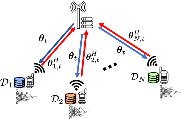
Figure 1: Illustration of the FL system model and the FedAvg algorithm.

I-A Preliminaries

The objective of FL is to solve the following optimization problem over $N$ clients

$$\min_{\boldsymbol{\theta}\in\mathbb{R}^{d}}f(\boldsymbol{\theta})=\frac{1}{N}\sum^{N}_{n=1}\underbrace{\mathds{E}_{\zeta_{n}\sim\mathcal{D}_{n}}f(\boldsymbol{\theta},\zeta_{n})}_{\mathrel{\mathop{:}}=f_{n}(\boldsymbol{\theta})},$$ (1)

where $\boldsymbol{\theta}\in\mathbb{R}^{d}$ denotes the model parameters, $\zeta_{n}$ is a random data sample, $\mathcal{D}_{n}$ denotes the dataset of client $n$, and $f$ is the problem specific empirical loss function. At each iteration of FL, each client aims to minimize its local loss function $f_{n}(\boldsymbol{\theta})$ using the stochastic gradient descent method. Then, the clients seek a consensus on the model with the help of the PS. The most widely used consensus strategy is to periodically average the locally optimized parameter models, which is referred to as federated averaging (FedAvg). The FedAvg procedure is summarized in Algorithm 1. See Fig. 1 for an illustration of the FL model across $N$ clients each with local dataset.

At the beginning of iteration $t$, each client pulls the current global parameter model $\boldsymbol{\theta}_{t}$ from the PS. In order to reduce the communication load, each client performs $H$ local updates before the consensus step, as illustrated in Algorithm 1 (lines 5-6), where

$$\mathbf{g}^{\tau}_{n,t}=\nabla_{\boldsymbol{\theta}}f_{n}(\boldsymbol{\theta}^{\tau-1}_{n,t},\zeta_{n,\tau})$$ (2)

is the gradient estimate of the $n$-th client at $\tau$-th local iteration based on the randomly sampled local data $\zeta_{n,\tau}$ and $\eta_{t}$ is the learning rate.

Algorithm 1 Federated Averaging (FedAvg)

1:for $t=1,2,\ldots$ do

2:     for $n=1,\ldots,N$ do in parallel

3:         Pull $\boldsymbol{\theta}_{t}$ from PS: $\boldsymbol{\theta}^{0}_{n,t}=\boldsymbol{\theta}_{t}$

4:         for $\tau=1,\ldots,H$ do

5:              Compute SGD: $\mathbf{g}^{\tau}_{n,t}=\nabla_{\boldsymbol{\theta}}f_{n}(\boldsymbol{\theta}^{\tau-1}_{n,t},\zeta_{n,\tau})$

6:              Update model: $\boldsymbol{\theta}^{\tau}_{n,t}=\boldsymbol{\theta}^{\tau-1}_{n,t}-\eta_{t}g^{\tau}_{n,t}$          

7:         Push $\boldsymbol{\theta}^{H}_{n,t}$      

8:     Federated Averaging: $\boldsymbol{\theta}_{t+1}=\frac{1}{|\mathcal{S}_{t}|}\sum_{n\in\mathcal{S}_{t}}\boldsymbol{\theta}^{H}_{n,t}$

We note that when $H=1$, clients can send their local gradient estimates instead of updated models, and this particular implementation is called federated SGD (FedSGD). For the sake of completeness, we also want to highlight that when the number of participating clients are large, e.g., FL across mobile devices, the PS can choose a subset of the clients for the consensus to reduce the communication overhead. However, in the scope of this work, we consider a scenario with a moderate number of clients, all of which participate in all the iterations of the learning process. This would be the case when the clients represent institutions, e.g., hospitals or banks; and hence, client selection is not required. Similarly, in the case of federated edge learning (FEEL) [13, 14, 15], the number of colocated wireless devices participating in the training process may be limited.

In addition to multiple local iterations, we can also employ compression of model updates in order to reduce the communication load from the clients to the PS at each iteration. Next, we briefly explain common compression strategies used in conveying the model updates from the clients to the PS in an efficient manner.

I-B Compressed Communication

The global model update in Algorithm 1 (line 8) can be equivalently written in the following form:

$$\boldsymbol{\theta}_{t+1}=\boldsymbol{\theta}_{t}+\frac{1}{N}\sum^{N}_{n=1}\underbrace{\sum^{H}_{\tau=1}-\eta_{t}\mathbf{g}^{\tau}_{n,t}}_{\Delta\boldsymbol{\theta}_{n,t}},$$ (3)

where we call the term $\Delta\boldsymbol{\theta}_{n,t}$ the model difference of the $n$th client at iteration $t$. Hence, each client can send the model difference instead of the updated model, and the compression is applied to this model difference. We can group the compression strategies into two main categories; namely, quantization and sparsification.

I-B1 Quantization

In general, floating point precision with 32 bits is used for training DNNs, thus 32 bits are required to represent each element of the local gradient estimate. Quantization techniques aims to represent each element with fewer bits to reduce the communication load [16, 17, 18, 19, 20, 21, 22, 23]. In the most extreme case, only the sign of each element can be sent, i.e., using only a single bit per dimension, to achieve up to $\times 32$ reduction in the communication load [16, 20, 21, 22]. Simulations with vision and speech recognition models show that significant reduction in the communication bandwidth can be achieved through quantization without much reduction in the network performance.

I-B2 Sparsification

Sparsification techniques transform a $d$ dimensional vector of gradient estimate $\mathbf{g}$ to its sparse representation $\tilde{\mathbf{g}}$, where the non-zero elements of $\tilde{\mathbf{g}}$ are equal to the corresponding elements of $\mathbf{g}$. Sparsification can be considered as applying a $d$-dimensional mask vector $\mathbf{m}\in\left\{0,1\right\}^{d}$ on $\mathbf{g}$; that is, $\tilde{\mathbf{g}}=\mathbf{m}\otimes\mathbf{g}$, where $\otimes$ denotes element-wise multiplication. We denote the sparsification ratio by $\phi$, i.e.,

$$\phi\triangleq\frac{||\mathbf{m}||_{1}}{d}<<1~{}.$$ (4)

It has been shown that it is possible to achieve sparsification ratios in the range of $\phi\in[0.01,0.001]$ for training dense DNN architectures, such as ResNet or VGG, without an apparent loss in test accuracy [24, 25, 26, 27, 28, 29, 30, 31, 32].

We also would like to remark that the three strategies mentioned above, i.e., multiple local updates, quantization, and sparsification, are orthogonal to each other, can be employed together to further reduce the required communication bandwidth in FL.

For collaborative/distributed learning, sparsification is commonly adopted in practice, and we identify its two popular variations in the literature: top-$K$ sparsification and rand-K sparsification [33]. Next, we briefly introduce the two approaches, and present their advantages and disadvantages in order to motivate the novel sparsification strategy we introduce in this work.

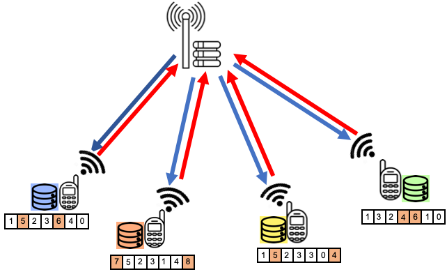
(a) Top-$K$ sparsification with $K=2$.

(b) Rand-$K$ sparsification with $K=2$.

Figure 2: Illustration of the top-$K$ and rand-$K$ sparsification strategies in FL. Vectors at each client represent the model update in an iteration. The colored entries represent the entries that are sent to the PS.

I-C Top-$K$ versus Rand-K Sparsification

In top-$K$ sparsification, each client constructs its own mask $\mathbf{m}_{n,t}$ independently, based on the greatest absolute values in $\Delta\boldsymbol{\theta}_{n,t}$. See Fig. 2(a) for an illustration of the top-$K$ sparsification strategy. Although top-$K$ sparsification is a promising compression strategy, its benefits in practical implementations are limited due to certain drawbacks. First, it requires a sorting operation which is computationally expensive when the size of the DNN architecture is large, which is the case when sparsification is most needed. Second, encoding and communication of the non-sparse locations induce additional overhead. Note that, when a client sends only $\phi d$ entries to the PS after sparsification, the compression ratio in terms of the communication bandwidth is less than $\phi$, since each client is required to send the locations of the all the non-zero parameters as well as their values for the PS to be able to recover the original update vector. More specifically, additional $\log_{2}d$ bits must be transmitted to the PS to represent the location of each non-zero parameter. We want to emphasize that this overhead becomes more significant when the sparsification strategy is combined with quantization; that is, if $q<\log_{2}d$ bits are used to represent the value of each non-zero parameter, then the communication of the non-zero positions becomes the main communication bottleneck. Finally, due to the mismatch between the masks of the clients, there might be a large gap between the sparsity in the uplink and downlink directions. We note that it has been shown in [34, 35] that it is possible to reduce the computational complexity of top-$K$ sparsification, hence in the scope of this paper we mainly focus on the last two drawbacks.
On the other hand, in rand-K sparsification, the sparsity mask is constructed randomly at each iteration. However, by using the same seed, all the clients can use the same random sparsification mask $\mathbf{m}_{t}$. See Fig. 2(b) for an illustration of the rand-$K$ sparsification strategy. Hence, one of the key advantages of rand-K compared to top-$K$, thanks to its pseudo-randomness, is that the clients do not need to encode and send the non-zero positions of their masks since they use an identical mask, which can also be known to the PS. In the case of distributed learning in a cloud center, this would allow using more efficient communication protocols that requires linearity, such as the allreduce operation [33, 36]. Similarly, in the case of FEEL, this would allow employing over-the-air computation in an efficient manner [13, 37, 38, 14]. Besides, rand-K, particularly its block-wise implementation, is more efficient compared to top-$K$ both in terms of computation and memory access complexity [33, 36]. Despite all the aforementioned advantages, rand-K sparsification introduces larger compression errors compared to top-$K$; and thus, performs poorly in the high compression regime [34, 33].
In the light of the above discussions, we emphasize that the optimal sparsification strategy depends on the scenario. For instance, when we consider distributed learning within a cluster with sufficiently fast connection, low compression rates are sufficient to scale distributed computation efficiently [39], hence rand-K might be the right option [33]. However, in FL, where clients are geographically separated and communicate with the PS over low-speed links, top-$K$ might be the only option.

I-D Sparse Network Architectures: Connections to Dynamic Network Pruning

Network pruning aims to reduce the size and complexity of DNNs [40, 41, 42, 43, 44, 45]. Given an initial DNN model $\boldsymbol{\theta}$, the objective of network pruning is to find a sparse version of $\boldsymbol{\theta}$, denoted by $\widetilde{\boldsymbol{\theta}}$, where only a small subset of the parameters are utilized with minimal loss in accuracy. In other words, the objective is to construct a $d$-dimensional mask vector $\mathbf{m}_{p}\in\left\{0,1\right\}^{d}$ to recover $\widetilde{\boldsymbol{\theta}}=\mathbf{m}_{p}\otimes\boldsymbol{\theta}$, where $||\mathbf{m}_{p}||_{1}<<d$. The ‘lottery ticket hypothesis’ [45] further states that such a mask can be employed throughout training to obtain the same level of accuracy with similar training time. We note that the existence of a “good” mask with $||\mathbf{m}_{p}||_{1}<<d$ and a similar test accuracy as the unpruned network implies the existence of a sparse communication strategy during training. If the optimal pruning mask $\mathbf{m}_{p}$ is used throughout training, this would also result in a significant reduction in the communication load by more than a factor of $\phi=||\mathbf{m}_{p}||_{1}/d$, as the clients need to convey only $||\mathbf{m}_{p}||_{1}$ values, and there is no need to specify their locations. However, the optimal pruning mask typically cannot be determined at the beginning of the training process. Alternatively, in dynamic network pruning [40, 41, 42, 43, 44], an evolving sequence of masks are employed over iterations, where the pruning mask employed at each iteration is updated gradually.

I-E Motivation and Contributions

At each iteration of the top-$K$ sparsification strategy, each client constructs a mask vector $\mathbf{m}_{n,t}$ from scratch, independently of the previous iterations, although the gradient values, and hence, the top-$K$ positions, exhibit certain correlation over time. The core idea of our work is to exploit this correlation to reduce the communication load resulting from the transmission of non-zero parameter locations. In other words, if the significant locations, those often observe large gradient values, were known, the clients could simply communicate the values corresponding to these locations without searching for the top-$K$ locations, or specifying their indices to the PS, reducing significantly both the communication load and the complexity.

More specifically, inspired by the dynamic pruning techniques [40, 41, 42, 43, 44], we propose a novel sparse communication strategy, called time correlated sparsification (TCS), where we search for a “good” global mask $\mathbf{m}_{t}$ to be used by all the clients at iteration $t$, which evolves gradually over iterations. Client $n$ uses a slightly personalized mask $\mathbf{m}_{n,t}$ based on the global mask $\mathbf{m}_{t}$, where

$$||\mathbf{m}_{n,t}-\mathbf{m}_{t}||_{1}=\epsilon_{t}<<\phi d.$$ (5)

This correlation between $\mathbf{m}_{n,t}$ and $\mathbf{m}_{t}$ helps to reduce the communication load since $\mathbf{m}_{t}$ is known at the PS. The small variations serve two purposes: First, they are used to ‘explore’ a small portion of new locations to improve the current mask. Second, certain locations may become significant temporarily due to the accumulation of errors when an error feedback mechanism is employed [25, 46, 47, 48, 49].

TCS is designed to benefit from the strong aspects of both the rand-K and top-$K$ sparsification strategies. The advantages of the proposed TCS strategy can be summarized as follows:

• Compared to top-$K$ sparsification, each client encodes and sends only a small number of non-sparse positions at each iteration, which reduces the number of transmitted bits. Furthermore, it makes high compression rates possible when TCS is combined with quantization.

• Although both TCS and top-$K$ offers the same sparsification level in the uplink direction, TCS achieves much higher sparsification level in the downlink direction thanks to the correlation of the masks across clients.

• Finally, since the individual masks mostly coincide, in a FEEL scenario, where the clients communicate with the PS over a shared wireless channel, TCS allows employing over-the-air computation in an efficient manner and takes advantage of the superposition property of the wireless medium [13, 37, 38, 14].

Through extensive simulations on the CIFAR-10 dataset, we show that TCS can achieve centralized training accuracy with $100$ times sparsification, and up to $2000$ times reduction in the communication load when employed together with quantization. We also note that, in the scope of this paper, we consider the general setup without any specification of the communication medium, and will consider the FEEL scenario with over-the-air computation in an extension of this work.

II Time Correlated Sparsification (TCS)

II-A Design principle

The main design principle behind TCS is employing two distinct mask vectors for sparsification. $\mathbf{m}_{global}$ is used to exploit previously identified important DNN parameters, whereas $\mathbf{m}_{local}$ explores new parameters. In particular, $\mathbf{m}_{global}$ is constructed based on the previous model update $\Delta{\boldsymbol{\theta}}$, motivated by the assumption that the most important DNN weights do not change significantly over iterations. Since all the clients receive the same global model update from the PS, mask vector $\mathbf{m}_{global}$ is identical for all the clients.
Let $\phi_{global}$ be the sparsification ratio for the mask $\mathbf{m}_{global}$ such that

$$||\mathbf{m}_{global}||_{1}=K_{global}=\phi_{global}\cdot d.$$ (6)

At the beginning of iteration $t$, each client receives the global model difference $\Delta\boldsymbol{\theta}_{t-1}$ from the PS, and accordingly, obtains $\mathbf{m}_{global}$ by simply identifying the top $K_{global}$ values in $|\Delta\boldsymbol{\theta}_{t-1}|$. In parallel, each client uses the received global model difference to recover $\boldsymbol{\theta}_{t}$.
Following the model update, each client $n\in[N]$ carries out the local SGD steps, and computes the local model difference $\Delta\boldsymbol{\theta}_{n,t}$. Finally, it obtains the sparse version of the local model difference, $\hat{\Delta}\boldsymbol{\theta}_{n,t}$, using the mask vector $\mathbf{m}_{global}$, i.e.,

$$\hat{\Delta}\boldsymbol{\theta}_{n,t}=\mathbf{m}_{global}\otimes\Delta\boldsymbol{\theta}_{n,t}.$$ (7)

We want to emphasize that since the PS sent out $\Delta{\boldsymbol{\theta}}_{t-1}$, mask vector $\mathbf{m}_{global}$ is known by the PS as well. Therefore, for each client it is sufficient to send only the non-zero values of $\hat{\Delta}\boldsymbol{\theta}_{n,t}$, without specifying their positions. Therefore, compared to the conventional top-$K$ sparsification framework, TCS further reduces the communication load by removing the need to communicate the positions of the non-zero values.
However, the main drawback of the above approach is that, if $\mathbf{m}_{global}$ is used throughout the training process, the same subset of weights will be used for model update at all iterations. Therefore, the proposed sparsification strategy requires a feedback mechanism in order to explore new weights at each iteration to check whether there are more important weights to consider for model update.
To introduce such a feedback mechanism, each client $n$ employs a second mask $\mathbf{m}^{n}_{local}$, which is unique to that client. The feedback mechanism works in the following way: given $\hat{\Delta}\boldsymbol{\theta}_{n,t}$, $\mathbf{m}^{n}_{local}$ is obtained as the vector of the greatest $K_{local}=\phi_{local}\cdot d$ entries of $|\Delta\boldsymbol{\theta}_{n,t}-\hat{\Delta}\boldsymbol{\theta}_{n,t}|$. Hence, at each iteration $t$, client $n$ sends, $n\in[N]$,

$$\widetilde{\Delta}\boldsymbol{\theta}_{n,t}=\Delta\boldsymbol{\theta}_{n,t}\otimes(\mathbf{m}_{global}+\mathbf{m}^{n}_{local})$$ (8)

to the PS.
Since the main purpose of $\mathbf{m}^{n}_{local}$ is to explore new important parameters, we assume that $\phi_{local}<<\phi_{global}$. Assume that $q$ bits are used to represent the value of each parameter. Then, using the global sparsification mask, the total number of bits to be conveyed to the PS is $K_{global}\cdot q$. For the feedback mechanism, in addition to $q$ bits to represent each of the parameter values, $\log_{2}d$ bits are required to inform the PS about each position of the parameter within the $d$-dimensional update vector. Hence, the total number of bits transmitted at each iteration is given by:

$$Q_{TCS}=q\cdot d\cdot(\phi_{local}+\phi_{global})+\log_{2}d\cdot d\cdot\phi_{local}.$$ (9)

Here, we would like to note that by utilizing a more efficient encoding strategy, it is possible to represent each position with $\log_{2}(1/\phi_{local})+2$ bits, instead of $\log_{2}d$, which is more communication efficient when $d$ is large. We refer the reader to Subsection II-E for the details of this encoding strategy. We want to emphasize that since $\phi_{local}<<\phi_{global}$, the proposed TCS strategy is more communication efficient than top-$K$ sparsification with the same $\phi_{global}$ value, such that $K=\phi_{global}\times d$. The total number of required bits are given as

$$Q_{topK}=d\cdot\phi_{global}\cdot(q+\log_{2}d).$$ (10)

One can easily observe that for $\phi_{local}<<\phi_{global}$, $Q_{TCS}$ is smaller than $Q_{topK}$, especially when $q$ is small.

II-B Error accumulation

Due to sparsification, there is an error in the local model difference sent to the PS by client $n$, which can be expressed as:

$$\mathbf{e}_{n,t}=\Delta\boldsymbol{\theta}_{n,t}\otimes(1-\mathbf{m}_{global}-\mathbf{m}^{n}_{local}).$$ (11)

It has been shown that the convergence speed can be improved by propagating the current compression error to next iterations [50, 46, 47]. That is, at iteration $t$, client $n$ intends to send

$$\bar{\Delta}\boldsymbol{\theta}_{n,t}=\Delta\boldsymbol{\theta}_{n,t}+\mathbf{e}_{n,t-1}$$ (12)

to the PS. Accordingly, each client performs sparsification on $\bar{\Delta}{\boldsymbol{\theta}}_{n,t}$ instead of $\Delta{\boldsymbol{\theta}}_{n,t}$. The overall TCS algorithm with error accumulation is summarized in Algorithm 2.

Algorithm 2 TCS with error accumulation

1:for $t=1,\ldots,T$ do

2:     Client side:

3:     for $n=1,\ldots,N$ do in parallel

4:         Receive $\Delta\boldsymbol{\boldsymbol{\theta}}_{t-1}$ from PS

5:         $\mathbf{m}_{global}=S_{top}(\Delta\boldsymbol{\theta}_{t-1},K_{global})$

6:         Update model: $\boldsymbol{\boldsymbol{\theta}}_{n,t}=\boldsymbol{\theta}_{n,t-1}+\Delta\boldsymbol{\theta}_{t-1}$

7:         Perform $H$ local updates and compute $\Delta{\boldsymbol{\theta}}_{n,t}$

8:         Error Feedback:

9:         $\bar{\Delta}{\boldsymbol{\theta}}_{n,t}=\Delta{\boldsymbol{\theta}}_{n,t}+\mathbf{e}_{n,t-1}$

10:         $\mathbf{m}^{n}_{local}=S_{top}(\bar{\Delta}{\boldsymbol{\theta}}_{n,t}\otimes(1-\mathbf{m}_{global}),K_{local})$

11:         $\widetilde{\Delta}\boldsymbol{\boldsymbol{\theta}}_{n,t}=(\mathbf{m}^{n}_{local}+\mathbf{m}_{global})\otimes\bar{\Delta}{\boldsymbol{\theta}}_{n,t}$

12:         Send $\widetilde{\Delta}\boldsymbol{\theta}_{n,t}$ to PS

13:         $\mathbf{e}_{n,t}=\bar{\Delta}\boldsymbol{\theta}_{n,t}-\widetilde{\Delta}\boldsymbol{\theta}_{n,t}$      

14:     Aggregate local model differences:

15:     $\Delta\boldsymbol{\theta}_{t}=\frac{1}{N}\sum_{n\in[N]}\widetilde{\Delta}\boldsymbol{\theta}_{n,t}$

16:     Send $\Delta\boldsymbol{\theta}_{t}$ to clients

We note that $S_{top}(\mathbf{v},K)$ in Algorithm 2 maps vector $\mathbf{v}\in\mathbb{R}^{d}$ to a mask vector $\mathbf{m}\in\left\{0,1\right\}^{d}$ such that if $\overline{v}_{K}$ is the $K$th greatest value in $|\mathbf{v}|$, then

$$\mathbf{m}_{i}=1~{}\text{if}~{}|\mathbf{v}_{i}|\geq\overline{v}_{K},$$ (13)

and $0$ otherwise.

II-C Layer-wise fairness

Due to the layered structure of the DNNs and the backpropagation mechanism, gradient values do not have uniform distribution across the layers. As a consequence, when top-$K$ sparsification is employed, the gradient of a weight belonging to initial layers is more likely to be chosen in the sparsified gradient. In other words, gradient values corresponding to later layers will be discarded more often, which may affect the final performance. Furthermore, at each iteration, by using a local mask vector $\mathbf{m}_{local}$, each client suggests $K_{local}$ new parameters to the PS to consider for sparsification, but again, we expect these locations to be distributed in a non-uniform manner across the DNN layers. To mitigate this problem, we introduce a layer-wise fairness constraint which introduces a distinct maximum sparsification ratio for each DNN layer in addition to the given sparsification parameters. The resultant scheme is called TCS with layer-wise fairness (TCS-LF).

Let the DNN architecture consist of $L$ layers, with $d_{l}$ parameters in the $l$-th layer, $l\in[L]$. The mask vectors are formed by concatenating $L$ mask vectors, each corresponding to a different layer. Let $\phi^{max}_{local}$ and $\phi^{max}_{global}$ denote the maximum sparsification levels allowed for the construction of the mask vectors $\mathbf{m}_{local}$ and $\mathbf{m}_{global}$, respectively. Similarly, let $\mathbf{m}^{l}_{local}$ and $\mathbf{m}^{l}_{global}$ denote the local and global mask vectors, respectively, for the $l$-th layer, $l\in[L]$. Then, the layer-wise fairness requiries

$$||\mathbf{m}^{l}_{global}||_{1}\geq\phi^{max}_{global}\cdot d_{l},~{}\forall l\in[L]$$ (14)

and

$$||\mathbf{m}^{n,l}_{local}||_{1}\geq\phi^{max}_{local}\cdot d_{l},~{}\forall l\in[L],~{}\forall n\in[N].$$ (15)

TCS-LF imposes a layer-wise sparsity constraint for both the clients ($\phi^{min}_{local}$) and the PS side ($\phi^{min}_{global}$) by including parameters from every individual layer of the network model. However, it is possible to consider fairness only at the PS side by only imposing the constraint $\phi^{min}_{global}$, which we call TCS with partial layer-wise fairness (TCS-PLF).

II-D TCS with momentum

Momentum SGD is a popular acceleration strategy used in training DNNs, and it increases the convergence speed and provides better generalization [51]. Here, we illustrate how momentum SGD optimizer can be incorporated into the FedSGD framework with the proposed sparsification strategy. We note that, momentum SGD can also be utilized when clients perform multiple local iterations [52, 53]; however, in the scope of this paper we limit our focus to FedSGD with momentum. In FedSGD with sparsification, each client sends sparsified gradient vector, $\widetilde{\mathbf{g}}_{n,t}$, and receives the sum of the sparsified gradients $\widetilde{\mathbf{g}}_{t}$ from the PS. When the momentum SGD is used for the model update, each user first updates the momentum term $\mathbf{w}_{n,t}$ as follows:

$$\mathbf{w}_{n,t}=\beta\cdot\mathbf{w}_{n,t-1}+\widetilde{\mathbf{g}}_{t-1},$$ (16)

where $\beta$ is the momentum coefficient. Following the update of the momentum term, the local model is updated using the momentum:

$$\boldsymbol{\theta}_{n,t}=\boldsymbol{\theta}_{n,t-1}+\eta_{t}\cdot\mathbf{w}_{n,t}.$$ (17)

We refer to the momentum term, $\mathbf{w}_{n,t}$, introduced above as the global momentum, since it is identical for all the clients. The overall TCS framework with global momentum is summarized in Algorithm 3.

Algorithm 3 TCS with global momentum

1:for $t=1,\ldots,T$ do

2:     Client side:

3:     for $n=1,\ldots,N$ do in parallel

4:         Receive $\tilde{\mathbf{g}}_{t-1}$ from PS

5:         $\mathbf{m}_{global}=S_{top}(\mathbf{g}_{t-1},K_{global})$

6:         Update momentum:

7:         $\mathbf{w}_{n,t}=\mathbf{w}_{n,t-1}+\beta\bar{\mathbf{g}}_{t-1}$

8:         Update model: $\boldsymbol{\theta}_{n,t}=\boldsymbol{\theta}_{n,t-1}-\eta_{t}\cdot\mathbf{w}_{n,t}$

9:         Compute SGD: $\mathbf{g}_{n,t}=\nabla_{\boldsymbol{\theta}}F(\boldsymbol{\theta}_{n,t},\zeta_{n,t})$

10:         $\bar{\mathbf{g}}_{n,t}=\mathbf{g}_{n,t}+\mathbf{e}_{n,t-1}$

11:         $\mathbf{m}^{n}_{local}=S_{top}(\bar{\mathbf{g}}_{n,t}\otimes(1-\mathbf{m}_{global}),K_{local})$

12:         $\widetilde{\mathbf{g}}_{n,t}=(\mathbf{m}^{n}_{local}+\mathbf{m}_{global})\otimes\bar{\mathbf{g}}_{n,t}$

13:         Send $\widetilde{\mathbf{g}}_{n,t}$ to PS

14:         $\mathbf{e}_{n,t}=\bar{\mathbf{g}}_{n,t}-\widetilde{\mathbf{g}}_{n,t}$      PS side:

15:     Aggregate local gradients:

16:     $\tilde{\mathbf{g}}_{t}=\frac{1}{N}\sum_{n\in[N]}\widetilde{\mathbf{g}}_{n,t}$

17:     Send $\tilde{\mathbf{g}}_{t}$ to clients

II-E Sparsity encoding

In this subsection, the position of the non-zero values. In general, $\log_{2}d$ bits are sufficient to send the position of each non-zero element of the vectors to be conveyed. However, for the local sparsification step based on $\mathbf{m}^{n}_{local}$, we employ the following coding scheme to send the position of the non-zero values. Let $\mathbf{v}$ be a sparse vector, where $\phi$ portion of its indices are non-zero. Initially, we assume $\mathbf{v}$ is divided into equal-length blocks of size $1/\phi$. The position of each non-zero value in $\mathbf{v}$ can be defined by two parameters; namely, BlockIndex and IntraBlockPosition which denotes the corresponding block and its position within the block, respectively. Hence, IntraBlockPosition can be represented with $\log_{2}(1/\phi)$ bits. To specify the BlockIndex two additional bits are sufficient. We use $0$ to identify the end of each block, and append $1$ to the beginning of the $\log_{2}(1/\phi)$ bits used for IntraBlockPosition. Hence, on average $\log_{2}(1/\phi)+2$ bits are needed to represent the location of each non-zero value.
In the decoding part, given the encoded binary vector $\mathbf{v}_{loc}$ for the position of the non-zero values in $\mathbf{v}$, the PS starts reading the bits from the first index and checks whether it is $0$ or $1$. If it is $1$, then the next $\log_{2}(1/\phi)$ bits are used to recover the position of the non-zero value in the current block. If the index is $0$, then the PS increases BlockIndex, which tracks the current block, by one, and moves on to the next index. The overall decoding procedure is illustrated in Algorithm 4.

Algorithm 4 Sparse position decoding

1:Input: Encoded sparse position vector $\mathbf{v}_{loc}$

2:Initialize: $pointer=0$

3:Initialize: $BlockIndex$

4:while $pointer<length(\mathbf{v}_{loc})$ do

5:     if $\mathbf{v}_{loc}(pointer)=0$ then

6:         $BlockIndex=BlockIndex+1$

7:         $pointer=pointer+1$

8:     else

9:         Read next $\log_{2}(1/\phi)$ bits for $IntraBlockPosition$

10:         Recover the location of a non-zero value:

11:         $(1/\phi)\cdot BlockIndex+IntraBlockPosition$

12:         $pointer=pointer+\log_{2}(1/\phi)+1$      

To elucidate the sparse encoding, consider a sparse vector $\mathbf{v}$ of size $d=12$ with $\phi=1/4$ and the indices of the non-zero values are given as $1,3,10$. Since $\phi=1/4$, the vector is divided into 3 blocks, each of size $4$ and IntraBlockPosition of each non-zero value can be represented by 2 bits, i.e., $00,10,01$; hence, overall the sparse representation can be written as a binary vector of

$$[{\color[rgb]{0,1,0}1}{\color[rgb]{1,0,0}00}{\color[rgb]{0,1,0}1}{\color[rgb]{1,0,0}10}{\color[rgb]{0,0,1}0}{\color[rgb]{0,0,1}0}{\color[rgb]{0,1,0}1}{\color[rgb]{1,0,0}01}{\color[rgb]{0,0,1}0}],$$ (18)

where the bits in red represents the position within the block, bits in green indicate that the following two bits refer to the position within the current block, and bits in blue represent the end of a block.

II-F Fractional quantization

There is already a rich literature on quantized communication in the distributed SGD framework [16, 17, 18, 19, 20, 21, 22]. Although the most common approaches are TernGrad [18] and QSGD [18], we consider the scaled sign operator [46, 16] for quantization. For a given $d$ dimensional vector $\mathbf{u}$, scaled sign operator maps the value of $i$th parameter, $\mathbf{u}_{i}$, to a quantized scalar value, $\mathcal{Q}(\mathbf{u}_{i})$, in the following way:

$$\mathcal{Q}(\mathbf{u}_{i})=\frac{||\mathbf{u}||_{1}}{d}\operatorname{sign}(\mathbf{u}_{i}),$$ (19)

where $\operatorname{sign}(\cdot)$ is the sign operator. It has been shown that the impact of the quantization error can be reduced by dividing $\mathbf{u}$ into $P$ smaller disjoint blocks $\left\{\mathbf{u}_{1},\ldots,\mathbf{u}_{P}\right\}$, and then applying quantization to each block separately, and often these blocks correspond to layers of DNN architecture [16]. Although we follow the same approach, inspired by the natural compression approach in [54], we utilize a different quantization scheme. Let $u_{max}$ and $u_{min}$ be the maximum and minimum values in vector $|\mathbf{u}|$, respectively. We divide the interval $[u_{max},u_{min}]$ into $P$ disjoint intervals $I_{1},\ldots,I_{P}$, such that the $p$th interval, $I_{p}$, is given as

$$I_{p}=[\sigma^{p-1}u_{max},\sigma^{p}u_{max}]$$ (20)

where,

$$\sigma=\left(\frac{u_{min}}{u_{max}}\right)^{1/P}.$$ (21)

Further, let $\mu_{p}$ be the average of the values assigned to interval $I_{p}$. Then fractional quantization maps the value of $i$th parameter, $\mathbf{u}_{i}$, to a quantized scalar value, $\mathcal{Q}_{f}(\mathbf{u}_{i})$, in the following way:

$$\mathcal{Q}_{f}(\mathbf{u}_{i})=\sum^{P}_{p=1}\mathds{1}_{\left\{\mathbf{u}_{i}\in I_{p}\right\}}\mu_{p}\operatorname{sign}(\mathbf{u}_{i}),$$ (22)

where $\mathds{1}_{\left\{\cdot\right\}}$ is the indicator function. Since there are $P$ intervals in total, $\log_{2}P$ bits are sufficient to identify the corresponding interval of $\mathbf{u}_{i}$, $i=1,\ldots,d$. An additional bit is sufficient to represent the sign, hence in total $\log_{2}P+1$ bit are required per parameter. Additional $32\cdot P$ bits are required to convey the mean values of the intervals. Consequently, for a given $d$ dimensional vector $\mathbf{u}$, a total of $d(\log_{2}P+1)+32\cdot P$ bits are required, and often the second term is negligible.
One can observe that fractional quantization strategy ensures the following inequality for each parameter value $\mathbf{u}_{i}$:

$$|\mathcal{Q}_{f}(\mathbf{u}_{i})-\mathbf{u}_{i}|\leq\gamma|\mathbf{u}_{i}|,$$ (23)

where $\gamma=\frac{1-\sigma}{\sigma}$. Accordingly, similar inequality holds for vector $\mathbf{u}$ and its quantized version $\tilde{\mathbf{u}}$ i.e.,

$$||\tilde{\mathbf{u}}-\mathbf{u}_{i}||_{2}\leq\gamma||\mathbf{u}_{i}||_{2}.$$ (24)

We remark that inequality (24) is often used to show the boundedness of the compression error, and to prove the convergence of distributed training with compression error [46]. Besides, as illustrated in inequality (23), fractional quantization also implies a proportional error for each parameter value, which provides a certain fairness among the parameters belonging to different layers of the DNN.

III Numerical Results

In this section, we provide numerical results compering all the introduced schemes above, and illustrate the remarkable improvements in the communication efficiency provided by TCS and its variants.

III-A Simulation Setup

To evaluate the performance of the proposed TCS strategy, we consider the image classification task on the CIFAR-10 dataset [55], which consists of 10 image classes, organized into 50K training and 10K test images, respectively. We employ the ResNet-18 architecture as the DNN [56], which consists of 8 basic blocks, each with two 3x3 convolutional layers and batch normalization. After two consecutive basic blocks, image size is halved with an additional 3x3 convolutional layer. This network consists of 11,173,962 trainable parameters altogether. We consider a network of $N=10$ clients and a federated setup, in which the training dataset is divided among the clients in a disjoint manner. The images, based on their classes, are distributed in an identically and independently distributed (IID) manner among the clients.

III-B Implementation

For performance evaluation, we consider the centralized training as our main benchmark, where we assume that all the training dataset is collected at one client. We set the batch size to 128 and the learning rate to $\eta=0.1$. The performance of this centralized setting will be referred to as the Baseline in our simulation results. For all the FL strategies considered in this work we set the batch size to 64, and adopt the linear learning rate scaling rule in [57], where the learning rate is scaled according to the cumulative batch size and the total number of samples trained by all the clients, taking the batch size of 128 as a reference value with the corresponding learning rate $\eta=0.1$. Hence, for our setup with $N=10$ clients, we use the learning rate $\eta=0.5$. Further, in all the FL implementations we employ the warm up strategy [57], where the learning rate is initially set to $\eta=0.1$, and is increased to its corresponding scaled value gradually in the first 5 epochs. We also note that during the warm up phase we do not employ sparsification and quantization methods for communication.
The DNN architecture is trained for 300 epochs and the learning rate is reduced by a factor of 10 after the first 150 and 225 epochs, respectively [58, 56]. Lastly, in all the simulations we employ L2 regularization with a given weight decay parameter $10^{-4}$.
For performance evaluation, we consider the top-$K$ sparsification scheme as a second benchmark. For top-$K$ sparsification we set the sparsification ratio to $\phi=10^{-2}$. Accordingly, for the proposed TCS strategy we set $\phi_{global}=10^{-2}$ and $\phi_{local}=10^{-3}$. We want to emphasize that for the TCS strategy with 10 clients, these parameters imply a maximum of $0.02$ sparsification ratio; in other words $\times 50$ compression in the PS-to-client direction as well, which is not the case for top-$K$ sparsification. For TCS-LF, we set $\phi^{min}_{local}=4\times 10^{-4}$ and $\phi^{min}_{global}=10^{-3}$ for the network layers and consider $\phi^{min}_{global}=10^{-3}$ for TCS-PFL as well.
We recall that one of the key design parameters of FL is the number of local steps $H$. Hence, we use TCS-L$H$ to denote the TCS scheme with $H$ local iterations and use TCS to refer to the FedSGD scheme where $H=1$. For FedAvg, we consider $H=2$ and $H=2$ in our simulations.
Finally, we also employ quantization strategy to represent each non-zero value with $q<<32$ bits and use the notation ‘Q$q$’ to denote the number of bits used to represent each element.For example, TCS-L4-Q5 denotes to $H=4$ along with 5-bit quantization. For performance evaluation, we employ two performance metrics: test accuracy and the bit budget, corresponding to the performance of the final trained model and the communication load, respectively. More specifically, the bit budget refers to the average number of bits conveyed from a client to the PS per parameter per iteration.

III-C Simulation Results

In our first simulation, we consider 8 schemes, namely the Baseline, top-$K$ sparsification, TCS, TCS-PLF, TCS-LF, TCS-L2, TCS-L4, and TCS-L4-Q5, where the first two are used as benchmark schemes. For each scheme we take the average over 5 trials. The final test accuracy results, with mean and standard deviation, and the bit budget for each scheme is presented in Table I. In Figure 3, we present the test accuracy results with respect to the epoch index.

Method	Test Accuracy (mean $\pm$ std)	Bit budget
TCS	92.44 $\pm$ 0.143	0.363
TCS-L2	92.578 $\pm$ 0.189	0.1815
TCS-L4	92.53 $\pm$ 0.22	0.0907
TCS-L4-Q5	92.485 $\pm$ 0.22	0.01675
TCS-PLF	92.142 $\pm$ 0.166	0.363
TCS-LF	92.115 $\pm$ 0.324	0.363
top-$K$	92.194 $\pm$ 0.247	0.41
Baseline	92.228 $\pm$ 0.232	-

TABLE I: Test accuracy (for $\eta=0.5$) and bit budget of the studied schemes.

We observe that the proposed TCS scheme requires $12\%$ lower bit budget than top-$K$ sparsification while achieving a higher average test accuracy. Similarly, it achieves approximately $\times 100$ reduction in the communication load without losing the accuracy. We also observe that TCS with multiple local iterations, in particular TCS-L2 and TCS-L4, achieve higher test accuracy compared to TCS with single local iteration. While the best accuracy achieved by TCS-L2, TCS-L4 achieves almost the same accuracy, but with half the average bit budget. Although this may seem counter-intuitive at the first glance, we remark that due to random batch sampling in SGD, gradient values behave as random variables, and hence, using model difference over $H$ iterations may provide a more accurate observation to be able to identify new important weights. To reduce the bit budget further we consider TCS-L4-Q5, where all the non-zero values are represented with 5 bits in total while one bit is used for the sign. We observe that TCS with quantization can achieve a $\times 2000$ reduction in the communication load, with an even better test accuracy compared to the centralized baseline.

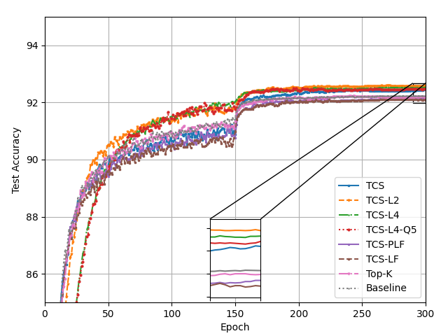
Figure 3: Comparison of the test accuracy results for different FL techniques and the centralized baseline over 300 epochs (for $\eta=0.5$).

Method	Test Accuracy (mean $\pm$ std)	Bit budget
TCS	92.094 $\pm$ 0.182	0.363
TCS-L4	92.62$\pm$ 0.0892	0.0907
TCS-L4-Q5	92.763 $\pm$ 0.210	0.01675
TCS-LF	92.481 $\pm$ 0.157	0.363
TCS-PLF	92.442 $\pm$ 0.189	0.363
TCS-LF-Q5	92.042 $\pm$ 0.173	0.067
top-$K$	91.856 $\pm$ 0.317	0.41
Baseline	92.228 $\pm$ 0.232	-

TABLE II: Test accuracy (for $\eta=0.8$) and bit budget of the studied schemes.

We observe that when $\eta=0.5$, layer-wise fairness (TCS-LF) does not improve the accuracy. We argue that the correlation over time may not be identical for all the layers, which requires more custom choice for the fairness constraints. We also remark that the efficiency of TCS and TCS-LF may depend on the learning rate. To analyze the impact of the learning rate $\eta$ on the performance of TCS and its variations with layer-wise fairness, we repeat our simulations with a learning rate of $\eta=0.8$ and report the results in Table II. The results show that, when the learning rate is increased, although the test accuracy of the TCS slightly reduces, its layer-wise fair variations TCS-LF and TCS-PLF perform better. Similarly to the previous simulation results with $\eta=0.5$, we observe that the highest test accuracy is achieved when TCS is implemented with multiple local steps.
We emphasize that the impact of quantization on the bit budget is more visible with TCS compared to top-$K$ sparsification. When quantization is used with top-$K$ sparsification, the number of bits used for the location becomes the bottleneck as quantization cannot reduce that. When TCS (with $\phi_{global}=10^{-2}$ and $\phi_{local}=10^{-3}$) is employed together with $5$-bit quantization, the corresponding bit budget is $0.067$ (bits per element). On the other hand, top-$K$ sparsification ($\phi=10^{-2}$) with $5$-bit quantization requires a bit budget of $0.14$, which is more than twice the bit budget of TCS. Furthermore, when the number of bits used for quantization decreases, TCS becomes more and more communication efficient.

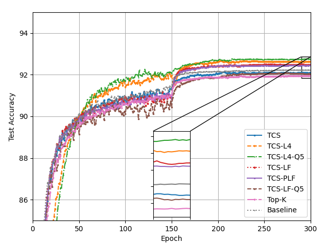
Figure 4: Comparison of the test accuracy results for different FL techniques and the centralized baseline over 300 epochs (for $\eta=0.8$).

Finally, we evaluate the performance of TCS with global momentum, introduced in Section II-D with parameter $\beta=0.9$, and compare it with the centralized baseline with momentum SGD. The final test accuracy results are presented in Table III and illustrated in Figure 5. The results show that TCS with global momentum achieves the same test accuracy result with the centralized baseline while providing $\times 100$ reduction in the communication load as before. Hence, we can conclude that momentum can be efficiently incorporated into the TCS framework.

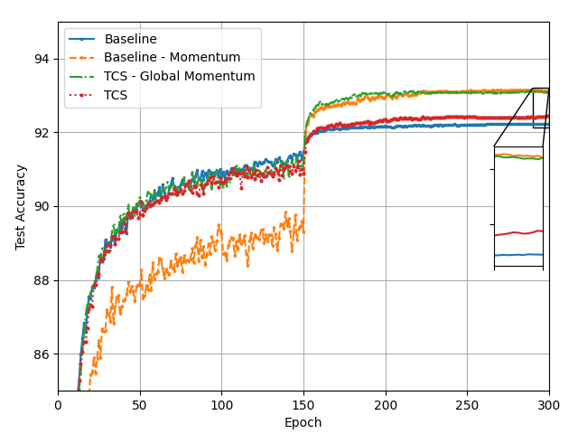
Figure 5: Comparison of the baseline and TCS strategies with and without momentum.

Method	Test Acc.
Baseline	92.23 $\pm$ 0.232
Baseline-Momentum	93.105 $\pm$ 0.346
TCS- Global Momentum	93.102 $\pm$ 0.182
TCS	92.44 $\pm$ 0.128

TABLE III: Test accuracy results of Baseline, Baseline with momentum, TCS with global m omentum and TCS.

IV Conclusion

In this paper, we introduced a novel sparse communication strategy for communication-efficient FL, called time correlated sparsification (TCS), by establishing an analogy between network pruning and gradient sparsification frameworks. The proposed strategy is built upon the assumption that at “important” locations the model difference (or the gradient) changes slowly over time, and utilizes this correlation over iterations to reduce the communication load. Through extensive simulations on CIFAR-10 dataset, we show that TCS can meet or even surpass the centralized baseline accuracy with $\times 100$ sparsification, and can reach up to $\times 2000$ reduction in the communication load when it is employed together with quantization. The proposed TCS strategy provides natural sparsification in the downlink communication as well. By employing a separate quantization operator at the PS, similarly to [48, 49, 23], the communication load for the downlink phase can be reduced further, which we will investigated in an extension of this work.

References

- [1] H. Buehler, L. Gonon, J. Teichmann, and B. Wood, “Deep hedging,” Quantitative Finance, vol. 19, no. 8, pp. 1271–1291, 2019.
- [2] M. J. Sheller, B. Edwards, G. A. Reina, and et al., “Federated learning in medicine: facilitating multi-institutional collaborations without sharing patient data,” in Scientific Reports, vol. 10, 28 Jul 2020.
- [3] F. Zerka, S. Barakat, S. Walsh, M. Bogowicz, R. T. H. Leijenaar, A. Jochems, B. Miraglio, D. Townend, and P. Lambin, “Systematic review of privacy-preserving distributed machine learning from federated databases in health care,” JCO Clinical Cancer Informatics, no. 4, pp. 184–200, 2020.
- [4] P. Trakadas, P. Simoens, P. Gkonis, L. Sarakis, A. Angelopoulos, A. P. Ramallo-González, A. Skarmeta, C. Trochoutsos, D. Calvo, T. Pariente, and et al., “An artificial intelligence-based collaboration approach in industrial iot manufacturing: Key concepts, architectural extensions and potential applications,” Sensors, vol. 20, no. 19, p. 5480, Sep 2020.
- [5] W. Li, F. Milletarì, D. Xu, N. Rieke, J. Hancox, W. Zhu, M. Baust, Y. Cheng, S. Ourselin, M. J. Cardoso, and A. Feng, “Privacy-preserving federated brain tumour segmentation,” in Machine Learning in Medical Imaging. Springer International Publishing, 2019, pp. 133–141.
- [6] C. J. Hoofnagle, B. van der Sloot, and F. Z. Borgesius, “The european union general data protection regulation: what it is and what it means,” Information & Communications Technology Law, vol. 28, no. 1, pp. 65–98, 2019.
- [7] N. Rieke, J. Hancox, W. Li, F. Milletari, H. Roth, S. Albarqouni, S. Bakas, M. N. Galtier, B. Landman, K. Maier-Hein, S. Ourselin, M. Sheller, R. M. Summers, A. Trask, D. Xu, M. Baust, and M. J. Cardoso, “The future of digital health with federated learning,” CoRR, vol. abs/2003.08119, 2020.
- [8] B. McMahan, E. Moore, D. Ramage, S. Hampson, and B. A. y Arcas, “Communication-Efficient Learning of Deep Networks from Decentralized Data,” in Proceedings of the 20th International Conference on Artificial Intelligence and Statistics, ser. Proceedings of Machine Learning Research, vol. 54, Fort Lauderdale, FL, USA, 20–22 Apr 2017, pp. 1273–1282.
- [9] K. Simonyan and A. Zisserman, “Very deep convolutional networks for large-scale image recognition,” in International Conference on Learning Representations, 2015.
- [10] D. Fohr, O. Mella, and I. Illina, “New Paradigm in Speech Recognition: Deep Neural Networks,” in IEEE International Conference on Information Systems and Economic Intelligence, Marrakech, Morocco, Apr. 2017. [Online]. Available: https://hal.archives-ouvertes.fr/hal-01484447
- [11] M. S. H. Abad, E. Ozfatura, D. GUndUz, and O. Ercetin, “Hierarchical federated learning across heterogeneous cellular networks,” in ICASSP 2020 - 2020 IEEE International Conference on Acoustics, Speech and Signal Processing (ICASSP), 2020, pp. 8866–8870.
- [12] S. Wang, T. Tuor, T. Salonidis, K. K. Leung, C. Makaya, T. He, and K. Chan, “Adaptive federated learning in resource constrained edge computing systems,” IEEE Journal on Selected Areas in Communications, vol. 37, no. 6, pp. 1205–1221, 2019.
- [13] M. Mohammadi Amiri and D. Gündüz, “Machine learning at the wireless edge: Distributed stochastic gradient descent over-the-air,” IEEE Transactions on Signal Processing, vol. 68, pp. 2155–2169, 2020.
- [14] M. M. Amiri and D. Gündüz, “Federated learning over wireless fading channels,” IEEE Transactions on Wireless Communications, vol. 19, no. 5, pp. 3546–3557, 2020.
- [15] D. Gunduz, D. B. Kurka, M. Jankowski, M. M. Amiri, E. Ozfatura, and S. Sreekumar, “Communicate to learn at the edge,” IEEE Communications Magazine, 2021.
- [16] S. Zheng, Z. Huang, and J. Kwok, “Communication-efficient distributed blockwise momentum SGD with error-feedback,” in Advances in Neural Information Processing Systems 32, 2019, pp. 11 450–11 460.
- [17] D. Alistarh, D. Grubic, J. Li, R. Tomioka, and M. Vojnovic, “QSGD: Communication-efficient SGD via gradient quantization and encoding,” in Advances in Neural Information Processing Systems 30, 2017, pp. 1709–1720.
- [18] W. Wen, C. Xu, F. Yan, C. Wu, Y. Wang, Y. Chen, and H. Li, “Terngrad: Ternary gradients to reduce communication in distributed deep learning,” in Advances in Neural Information Processing Systems 30, 2017, pp. 1509–1519.
- [19] J. Wu, W. Huang, J. Huang, and T. Zhang, “Error compensated quantized SGD and its applications to large-scale distributed optimization,” in Proceedings of the 35th International Conference on Machine Learning, Stockholmsmässan, Stockholm Sweden, Jul 2018, pp. 5325–5333.
- [20] J. Bernstein, Y.-X. Wang, K. Azizzadenesheli, and A. Anandkumar, “signSGD: Compressed optimisation for non-convex problems,” in Proceedings of the 35th International Conference on Machine Learning, Stockholmsmässan, Stockholm Sweden, Jul 2018, pp. 560–569.
- [21] J. Bernstein, J. Zhao, K. Azizzadenesheli, and A. Anandkumar, “signSGD with majority vote is communication efficient and fault tolerant,” in International Conference on Learning Representations, 2019.
- [22] F. Seide, H. Fu, J. Droppo, G. Li, and D. Yu, “1-bit stochastic gradient descent and application to data-parallel distributed training of speech dnns,” in Interspeech 2014, September 2014.
- [23] M. M. Amiri, D. Gündüz, S. R. Kulkarni, and H. V. Poor, “Federated learning with quantized global model updates,” CoRR, vol. abs/2006.10672, 2020.
- [24] Y. Lin, S. Han, H. Mao, Y. Wang, and B. Dally, “Deep gradient compression: Reducing the communication bandwidth for distributed training,” in International Conference on Learning Representations, 2018.
- [25] S. U. Stich, J.-B. Cordonnier, and M. Jaggi, “Sparsified SGD with memory,” in Advances in Neural Information Processing Systems 31, 2018, pp. 4448–4459.
- [26] D. Alistarh, T. Hoefler, M. Johansson, N. Konstantinov, S. Khirirat, and C. Renggli, “The convergence of sparsified gradient methods,” in Advances in Neural Information Processing Systems 31, 2018, pp. 5976–5986.
- [27] J. Wangni, J. Wang, J. Liu, and T. Zhang, “Gradient sparsification for communication-efficient distributed optimization,” in Advances in Neural Information Processing Systems 31, 2018, pp. 1305–1315.
- [28] A. F. Aji and K. Heafield, “Sparse communication for distributed gradient descent,” in Proceedings of the 2017 Conference on Empirical Methods in Natural Language Processing. Copenhagen, Denmark: Association for Computational Linguistics, Sep. 2017, pp. 440–445.
- [29] S. Shi, Q. Wang, K. Zhao, Z. Tang, Y. Wang, X. Huang, and X. Chu, “A distributed synchronous SGD algorithm with global top-k sparsification for low bandwidth networks,” in 2019 IEEE 39th International Conference on Distributed Computing Systems (ICDCS), 2019, pp. 2238–2247.
- [30] P. Jiang and G. Agrawal, “A linear speedup analysis of distributed deep learning with sparse and quantized communication,” in Advances in Neural Information Processing Systems 31, 2018, pp. 2529–2540.
- [31] L. P. Barnes, H. A. Inan, B. Isik, and A. Ozgur, “rtop-k: A statistical estimation approach to distributed SGD,” CoRR, vol. 2005.10761, 2020.
- [32] F. Sattler, S. Wiedemann, K. Müller, and W. Samek, “Robust and communication-efficient federated learning from non-i.i.d. data,” IEEE Transactions on Neural Networks and Learning Systems, pp. 1–14, 2019.
- [33] N. F. Eghlidi and M. Jaggi, “Sparse communication for training deep networks,” CoRR, vol. abs/2009.09271, 2020.
- [34] S. Shi, X. Chu, K. C. Cheung, and S. See, “Understanding top-k sparsification in distributed deep learning,” CoRR, vol. abs/1911.08772, 2019.
- [35] V. Gupta, D. Choudhary, P. T. P. Tang, X. Wei, X. Wang, Y. Huang, A. Kejariwal, K. Ramchandran, and M. W. Mahoney, “Fast distributed training of deep neural networks: Dynamic communication thresholding for model and data parallelism,” CoRR, vol. abs/2010.08899, 2020.
- [36] C. Xie, S. Zheng, O. Koyejo, I. Gupta, M. Li, and H. Lin, “CSER: Communication-efficient SGD with error reset,” ArXiv, vol. abs/2007.13221, 2020.
- [37] G. Zhu, Y. Wang, and K. Huang, “Broadband analog aggregation for low-latency federated edge learning,” IEEE Trans. Wireless Comms., 2019.
- [38] T. Sery and K. Cohen, “On analog gradient descent learning over multiple access fading channels,” IEEE Trans. Signal Proc., vol. 68, pp. 2897–2911, 2020.
- [39] Z. Zhang, C. Chang, H. Lin, Y. Wang, R. Arora, and X. Jin, “Is network the bottleneck of distributed training?” in Proceedings of the Workshop on Network Meets AI I& ML, ser. NetAI ’20. New York, NY, USA: Association for Computing Machinery, 2020, p. 8–13.
- [40] H. Mostafa and X. Wang, “Parameter efficient training of deep convolutional neural networks by dynamic sparse reparameterization,” in Proceedings of the 36th International Conference on Machine Learning, Long Beach, California, USA, Jun 2019, pp. 4646–4655.
- [41] T. Dettmers and L. Zettlemoyer, “Sparse networks from scratch: Faster training without losing performance,” CoRR, vol. abs/1907.04840, 2019.
- [42] T. Lin, S. U. Stich, L. Barba, D. Dmitriev, and M. Jaggi, “Dynamic model pruning with feedback,” in International Conference on Learning Representations, 2020.
- [43] U. Evci, T. Gale, J. Menick, P. S. Castro, and E. Elsen, “Rigging the lottery: Making all tickets winners,” in Proceedings of the 37th International Conference on Machine Learning, ser. Proceedings of Machine Learning Research, vol. 119, Virtual, 13–18 Jul 2020, pp. 2943–2952.
- [44] X. Dai, H. Yin, and N. K. Jha, “Nest: A neural network synthesis tool based on a grow-and-prune paradigm,” CoRR, vol. abs/1711.02017, 2017.
- [45] J. Frankle and M. Carbin, “The lottery ticket hypothesis: Finding sparse, trainable neural networks,” in International Conference on Learning Representations, 2019.
- [46] S. P. Karimireddy, Q. Rebjock, S. Stich, and M. Jaggi, “Error feedback fixes SignSGD and other gradient compression schemes,” in Proceedings of the 36th International Conference on Machine Learning, Long Beach, California, USA, Jun 2019, pp. 3252–3261.
- [47] J. Wu, W. Huang, J. Huang, and T. Zhang, “Error compensated quantized SGD and its applications to large-scale distributed optimization,” in Proceedings of the 35th International Conference on Machine Learning, Stockholmsmässan, Stockholm Sweden, Jul 2018, pp. 5325–5333.
- [48] H. Tang, C. Yu, X. Lian, T. Zhang, and J. Liu, “DoubleSqueeze: Parallel stochastic gradient descent with double-pass error-compensated compression,” in Proceedings of the 36th International Conference on Machine Learning, Long Beach, California, USA, Jun 2019, pp. 6155–6165.
- [49] Y. Yu, J. Wu, and L. Huang, “Double quantization for communication-efficient distributed optimization,” in Advances in Neural Information Processing Systems 32, 2019, pp. 4438–4449.
- [50] F. Seide, H. Fu, J. Droppo, G. Li, and D. Yu, “1-bit stochastic gradient descent and application to data-parallel distributed training of speech dnns,” in Interspeech 2014, September 2014.
- [51] I. Sutskever, J. Martens, G. Dahl, and G. Hinton, “On the importance of initialization and momentum in deep learning,” ser. Proceedings of Machine Learning Research, vol. 28, no. 3. Atlanta, Georgia, USA: PMLR, 17–19 Jun 2013, pp. 1139–1147.
- [52] J. Wang, V. Tantia, N. Ballas, and M. Rabbat, “SLOWMO: Improving communication-efficient distributed SGD with slow momentum,” in International Conference on Learning Representations, 2020.
- [53] E. Ozfatura, K. Ozfatura, and D. Gunduz, “FedADC: Accelerated federated learning with drift control,” CoRR, vol. abs/2012.09102, 2020.
- [54] S. Horvath, C. Ho, L. Horvath, A. N. Sahu, M. Canini, and P. Richtárik, “Natural compression for distributed deep learning,” CoRR, vol. abs/1905.10988, 2019.
- [55] A. Krizhevsky, V. Nair, and G. Hinton, “Cifar-10 (canadian institute for advanced research).” [Online]. Available: http://www.cs.toronto.edu/ kriz/cifar.html
- [56] K. He, X. Zhang, S. Ren, and J. Sun, “Identity mappings in deep residual networks,” in Computer Vision – ECCV 2016, B. Leibe, J. Matas, N. Sebe, and M. Welling, Eds. Cham: Springer International Publishing, 2016, pp. 630–645.
- [57] P. Goyal, P. Dollár, R. B. Girshick, P. Noordhuis, L. Wesolowski, A. Kyrola, A. Tulloch, Y. Jia, and K. He, “Accurate, large minibatch SGD: training imagenet in 1 hour,” CoRR, vol. abs/1706.02677, 2017.
- [58] K. He, X. Zhang, S. Ren, and J. Sun, “Deep residual learning for image recognition,” in 2016 IEEE Conference on Computer Vision and Pattern Recognition (CVPR), 2016, pp. 770–778.