PyGlove: Symbolic Programming
for Automated Machine Learning
Abstract
Neural networks are sensitive to hyper-parameter and architecture choices. Automated Machine Learning (AutoML) is a promising paradigm for automating these choices. Current ML software libraries, however, are quite limited in handling the dynamic interactions among the components of AutoML. For example, efficient NAS algorithms, such as ENAS [1] and DARTS [2], typically require an implementation coupling between the search space and search algorithm, the two key components in AutoML. Furthermore, implementing a complex search flow, such as searching architectures within a loop of searching hardware configurations, is difficult. To summarize, changing the search space, search algorithm, or search flow in current ML libraries usually requires a significant change in the program logic.
In this paper, we introduce a new way of programming AutoML based on symbolic programming. Under this paradigm, ML programs are mutable, thus can be manipulated easily by another program. As a result, AutoML can be reformulated as an automated process of symbolic manipulation. With this formulation, we decouple the triangle of the search algorithm, the search space and the child program. This decoupling makes it easy to change the search space and search algorithm (without and with weight sharing), as well as to add search capabilities to existing code and implement complex search flows. We then introduce PyGlove, a new Python library that implements this paradigm. Through case studies on ImageNet and NAS-Bench-101, we show that with PyGlove users can easily convert a static program into a search space, quickly iterate on the search spaces and search algorithms, and craft complex search flows to achieve better results.
1 Introduction
Neural networks are sensitive to architecture and hyper-parameter choices [3, 4]. For example, on the ImageNet dataset [5], we have observed a large increase in accuracy thanks to changes in architectures, hyper-parameters, and training algorithms, from the seminal work of AlexNet [5] to recent state-of-the-art models such as EfficientNet [6]. However, as neural networks become increasingly complex, the potential number of architecture and hyper-parameter choices becomes numerous. Hand-crafting neural network architectures and selecting the right hyper-parameters is, therefore, increasingly difficult and often take months of experimentation.
Automated Machine Learning (AutoML) is a promising paradigm for tackling this difficulty. In AutoML, selecting architectures and hyper-parameters is formulated as a search problem, where a search space is defined to represent all possible choices and a search algorithm is used to find the best choices. For hyper-parameter search, the search space would specify the range of values to try. For architecture search, the search space would specify the architectural configurations to try. The search space plays a critical role in the success of neural architecture search (NAS) [7, 8], and can be significantly different from one application to another [9, 8, 10, 11]. In addition, there are also many different search algorithms, such as random search [12], Bayesian optimization [13], RL-based methods [9, 1, 14, 15], evolutionary methods [16], gradient-based methods [2, 17, 10] and neural predictors [18].
This proliferation of search spaces and search algorithms in AutoML makes it difficult to program with existing software libraries. In particular, a common problem of current libraries is that search spaces and search algorithms are tightly coupled, making it hard to modify search space or search algorithm alone. A practical scenario that arises is the need to upgrade a search algorithm while keeping the rest of the infrastructure the same. For example, recent years have seen a transition from AutoML algorithms that train each model from scratch [9, 8] to those that employ weight-sharing to attain massive efficiency gains, such as ENAS and DARTS [1, 2, 14, 19, 15]. Yet, upgrading an existing search space by introducing weight-sharing requires significant changes to both the search algorithm and the model building logic, as we will see in Section 2.2. Such coupling between search spaces and search algorithms, and the resulting inflexibility, impose a heavy burden on AutoML researchers and practitioners.
We believe that the main challenge lies in the programming paradigm mismatch between existing software libraries and AutoML. Most existing libraries are built on the premise of immutable programs, where a fixed program is used to process different data. On the contrary, AutoML requires programs (i.e. model architectures) to be mutable, as they must be dynamically modified by another program (i.e. the search algorithm) whose job is to explore the search space. Due to this mismatch, predefined interfaces for search spaces and search algorithms struggle to accommodate unanticipated interactions, making it difficult to try new AutoML approaches. Symbolic programming, which originated from LISP [20], provides a potential solution to this problem, by allowing a program to manipulate its own components as if they were plain data [21]. However, despite its long history, symbolic programming has not yet been widely explored in the ML community.
In this paper, we reformulate AutoML as an automated process of manipulating ML programs symbolically. Under this formulation, programs are mutable objects which can be cloned and modified after their creation. These mutable objects can express standard machine learning concepts, from a convolutional unit to a complex user-defined training procedure. As a result, all parts of a ML program are mutable. Moreover, through symbolic programming, programs can modify programs. Therefore the interactions between the child program, search space, and search algorithm are no longer static. We can mediate them or change them via meta-programs. For example, we can map the search space into an abstract view which is understood by the search algorithm, translating an architectural search space into a super-network that can be optimized by efficient NAS algorithms.
Further, we propose PyGlove, a library that enables general symbolic programming in Python, as an implementation of our method tested on real-world AutoML scenarios. With PyGlove, Python classes and functions can be made mutable through brief Python annotations, which makes it much easier to write AutoML programs. PyGlove allows AutoML techniques to be easily dropped into preexisting ML pipelines, while also benefiting open-ended research which requires extreme flexibility.
To summarize, our contributions are the following:
-
•
We reformulate AutoML under the symbolic programming paradigm, greatly simplifying the programming interface for AutoML by accommodating unanticipated interactions among the child programs, search spaces and search algorithms via a mutable object model.
-
•
We introduce PyGlove, a general symbolic programming library for Python which implements our symbolic formulation of AutoML. With PyGlove, AutoML can be easily dropped into preexisting ML programs, with all program parts searchable, permitting rapid exploration on different dimensions of AutoML.
-
•
Through case studies, we demonstrate the expressiveness of PyGlove in real-world search spaces. We demonstrate how PyGlove allows AutoML researchers and practitioners to change search spaces, search algorithms and search flows with only a few lines of code.
2 Symbolic Programming for AutoML
Many AutoML approaches (e.g., [9, 22, 2]) can be formulated as three interacting components: the child program, the search space, and the search algorithm. AutoML’s goal is to discover a performant child program (e.g., a neural network architecture or a data augmentation policy) out of a large set of possibilities defined by the search space. The search algorithm accomplishes the said goal by iteratively sampling child programs from the search space. Each sampled child program is then evaluated, resulting in a numeric measure of its quality. This measure is called the reward111While we use RL concepts to illustrate the core idea of our method, as will be shown later, the proposed paradigm is applicable to other types of AutoML methods as well.. The reward is then fed back to the search algorithm to improve future sampling of child programs.
In typical AutoML libraries [23, 24, 25, 26, 27, 28, 29, 30, 31], these three components are usually tightly coupled. The coupling between these components means that we cannot change the interactions between them unless non-trivial modifications are made. This limits the flexibility of the libraries. Some successful attempts have been made to break these couplings. For example, Vizier [26] decouples the search space and the search algorithm by using a dictionary as the search space contract between the child program and the search algorithm, resulting in modular black-box search algorithms. Another example is the NNI library [27], which tries to unify search algorithms with and without weight sharing by carefully designed APIs. This paper, however, solves the coupling problem in a different and more general way: with symbolic programming, programs are allowed to be modified by other programs. Therefore, instead of solving fixed couplings, we allow dynamic couplings through a mutable object model. In this section, we will explain our method and show how this makes AutoML programming more flexible.
2.1 AutoML as an Automated Symbolic Manipulation Process
AutoML can be interpreted as an automated process of searching for a child program from a search space to maximize a reward. We decompose this process into a sequence of symbolic operations. A (regular) child program (Figure 1-a) is symbolized into a symbolic child program (Figure 1-b), which can be then cloned and modified. The symbolic program is further hyperified into a search space (Figure 1-c) by replacing some of the fixed parts with to-be-determined specifications. During the search, the search space is materialized into different child programs (Figure 1-d) based on search algorithm decisions, or can be rewritten into a super-program (Figure 1-e) to apply complex search algorithms such as efficient NAS.
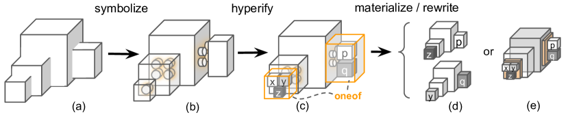
An analogy to this process is to have a robot build a house with LEGO [32] bricks to meet a human being’s taste: symbolizing a regular program is like converting molded plastic parts into LEGO bricks; hyperifying a symbolic program into a search space is like providing a blueprint of the house with variations. With the help of the search algorithm, the search space is materialized into different child programs whose rewards are fed back to the search algorithm to improve future sampling, like a robot trying different ways to build the house and gradually learning what humans prefer.
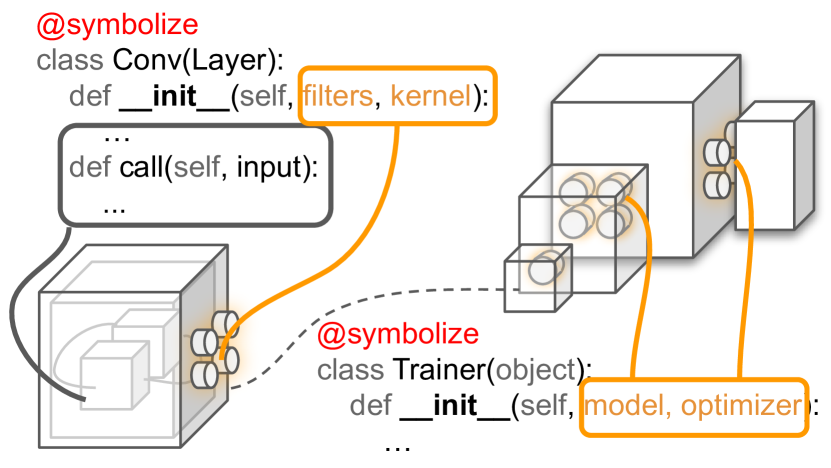
Symbolization.
A (regular) child program can be described as a complex object, which is a composition of its sub-objects. A symbolic child program is such a composition whose sub-objects are no longer tied together forever, but are detachable from each other hence can be replaced by other sub-objects. The symbolic object can be hierarchical, forming a symbolic tree which can be manipulated or executed. A symbolic object is manipulated through its hyper-parameters, which are like the studs of a LEGO brick, interfacing connections with other bricks. However, symbolic objects, unlike LEGO bricks, can have internal states which are automatically recomputed upon modifications. For example, when we change the dataset of a trainer, the train steps will be recomputed from the number of examples in the dataset if the training is based on the number of epochs. With such a mutable object model, we no longer need to create objects from scratch repeatedly, or modify the producers up-stream, but can clone existing objects and modify them into new ones. The symbolic tree representation puts an emphasis on manipulating the object definitions, while leaving the implementation details behind. Figure 2 illustrates the symbolization process.
2.2 Disentangling AutoML through Symbolic Programming
Disentangling search spaces from child programs.
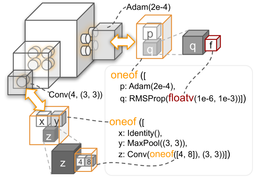
The search space can be disentangled from the child program in that 1) the classes and functions of the child program can be implemented without depending on any AutoML library (Appendix B.1.1), which applies to most preexisting ML projects whose programs were started without taking AutoML in mind; 2) a child program can be manipulated into a search space without modifying its implementation. Figure 4 shows that a child program is turned into a search space by replacing a fixed Conv with a choice of Identity, MaxPool and Conv with searchable filter size. Meanwhile, it swaps a fixed Adam optimizer with a choice between the Adam and an RMSProp with a searchable learning rate.
Disentangling search spaces from search algorithms.
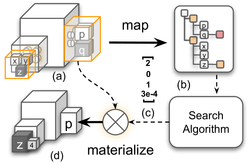
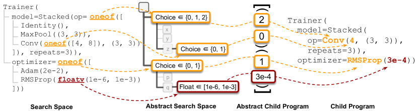
Symbolic programming breaks the coupling between the search space and the search algorithm by preventing the algorithm from seeing the full search space specification. Instead, the algorithm only sees what it needs to see for the purposes of searching. We refer to the algorithm’s view of the search space as the abstract search space. The full specification, in contrast, will be called the concrete search space (or just the “search space” outside this section). The distinction between the concrete and abstract search space is illustrated in Figure 4: the concrete search space acts as a boilerplate for producing concrete child programs, which holds all the program details (e.g., the fixed parts). However, the abstract search space only sees the parts that need decisions, along with their numeric ranges. Based on the abstract search space, an abstract child program is proposed, which can be static numeric values or variables. The static form is for obtaining a concrete child program, shown in Figure 4, while the variable form is used for making a super-program used in efficient NAS – the variables can be either discrete for RL-based use cases or real-valued vectors for gradient-based methods. Mediated by the abstract search space and the abstract child program, the search algorithm can be thoroughly decoupled from the child program. Figure 5 gives a more detailed illustration of Figure 4.
Disentangling search algorithms from child programs.
While many search algorithms can be implemented by rewriting symbolic objects, complex algorithms such as ENAS [1], DARTS [2] and TuNAS [15] can be decomposed into 1) a child-program-agnostic algorithm, plus 2) a meta-program (e.g. a Python function) which rewrites the search space into a representation required by the search algorithm. The meta-program only manipulates the symbols which are interesting to the search algorithm and ignores the rest. In this way, we can decouple the search algorithm from the child program.
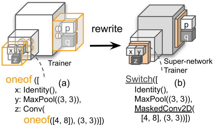
For example, the TuNAS [15] algorithm can be decomposed into 1) an implementation of REINFORCE [33] and 2) a rewrite function which transforms the architecture search space into a super-network, and replaces the regular trainer with a trainer that samples and trains the super-network, illustrated in Figure 6. If we want to switch the search algorithm to DARTS [2], we use a different rewrite function that generates a super-network with soft choices, and replace the trainer with a super-network trainer that updates the choice weights based on the gradients.
2.3 Search space partitioning and complex search flows
Early work [34, 35, 19] shows that factorized search can help partition the computation for optimizing different parts of the program. Yet, complex search flows have been less explored, possibly due in part to their implementation complexity. The effort involved in partitioning a search space and coordinating the search algorithms is usually non-trivial. However, the symbolic tree representation makes search space partitioning a much easier task: with a partition function, we can divide those to-be-determined parts into different groups and optimize each group separately. As a result, each optimization process sees only a portion of the search space – a sub-space – and they work together to optimize the complete search space. Section 3.4 discusses common patterns of such collaboration and how we express complex search flows.
3 AutoML with PyGlove
In this section, we introduce PyGlove, a general symbolic programming library on Python, which also implements our method for AutoML. With examples, we demonstrate how a regular program is made symbolically programmable, then turned into search spaces, searched with different search algorithms and flows in a dozen lines of code.
| Projects | Original lines of code | Modified lines of code |
| PyTorch ResNet [36] | 353 | 15 |
| TensorFlow MNIST [37] | 120 | 24 |
3.1 Symbolize a Python program
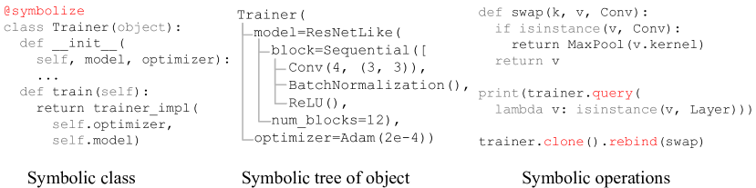
In PyGlove, preexisting Python programs can be made symbolically programmable with a symbolize decorator. Besides classes, functions can be symbolized too, as discussed in Appendix B.1.2. To facilitate manipulation, PyGlove provides a wide range of symbolic operations. Among them, query, clone and rebind are of special importance as they are foundational to other symbolic operations. Examples of these operations can be found in Appendix B.2. Figure 7 shows (1) a symbolic Python class, (2) an instance of the class as a symbolic tree, and (3) key symbolic operations which are applicable to a symbolic object. To convey the amount of work required to drop PyGlove into real-life projects, we show the number of lines of code in making a PyTorch [36] and a TensorFlow [37] projects searchable in Table 1.
3.2 From a symbolic program to a search space
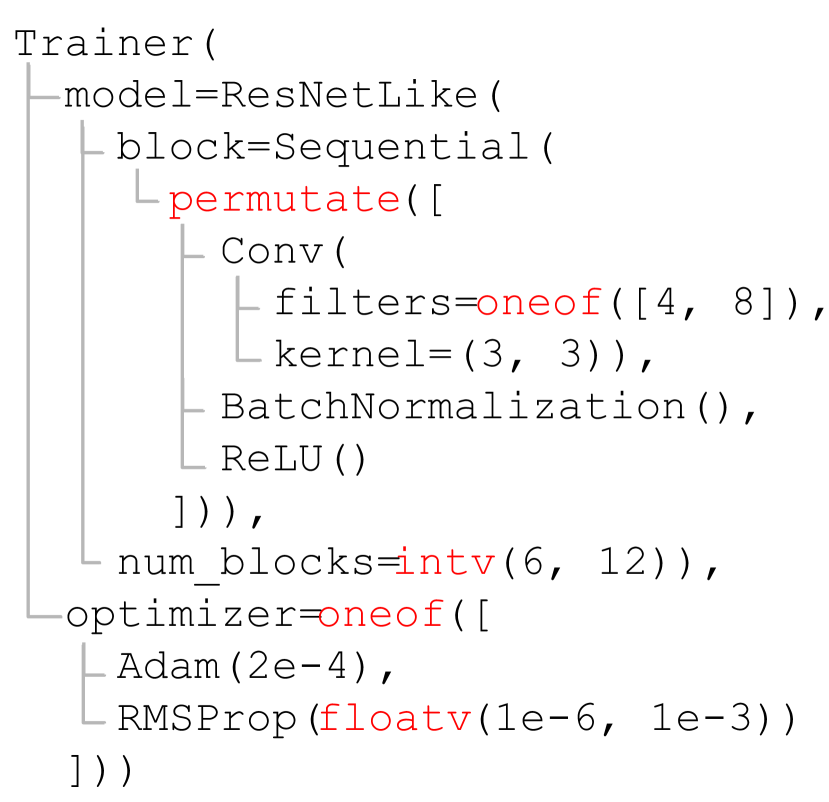
With a child program being a symbolic tree, any node in the tree can be replaced with a to-be-determined specification, which we call hyper value (in correspondence to hyperify, a verb introduced in Section 2.1 in making search spaces). A search space is naturally represented as a symbolic tree with hyper values. In PyGlove, there are three classes of hyper values: 1) a continuous value declared by floatv; 2) a discrete value declared by intv; and 3) a categorical value declared by oneof, manyof or permutate. Table 2 summarizes different hyper value classes with their semantics. Figure 9 shows a search space that jointly optimizes a model and an optimizer. The model space is a number of blocks whose structure is a sequence of permutation from [Conv, BatchNormalization, ReLU] with searchable filter size.
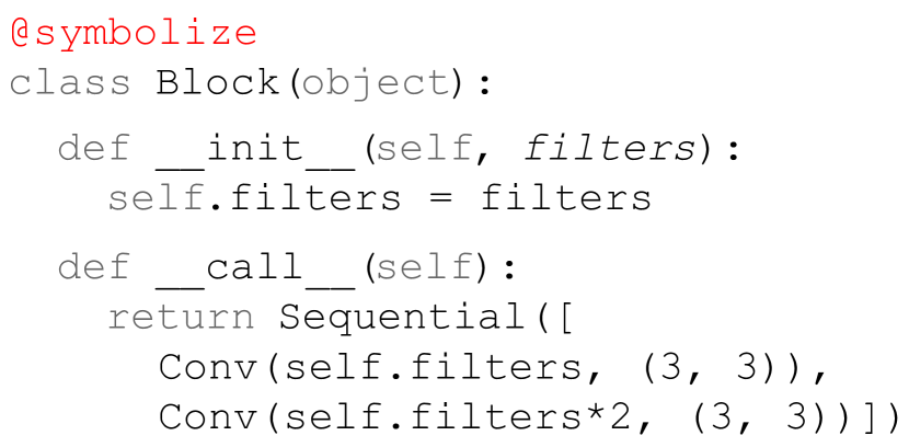
Dependent hyper-parameters can be achieved by using higher-order symbolic objects. For example, if we want to search for the filters of a Conv, which follows another Conv whose filters are twice the input filters, we can create a symbolic Block class, which takes only one filter size – the output filters of the first Conv – as its hyper-parameters. When it’s called, it returns a sequence of 2 Conv units based on its filters, as shown in Figure 9. The filters of the block can be a hyper value at construction time, appearing as a node in the symbolic tree, but will be materialized when it’s called.
3.3 Search algorithms
Without interacting with the child program and the search space directly, the search algorithm in PyGlove repeatedly 1) proposes an abstract child program based on the abstract search space and 2) receives measured qualities for the abstract child program to improve future proposals. PyGlove implements many search algorithms, including Random Search, PPO and Regularized Evolution.
| Strategy | Hyper-parameter annotation | Search space semantics |
| Continuous | floatv(min, max) | A float value from |
| Discrete | intv(min, max) | An int value from |
| Categorical | oneof(candidates) | Choose 1 out of N candidates |
| manyof(K, candidates, ) | Choose K out of N candidates with optional constraints on the uniqueness and order of chosen candidates | |
| permutate(candidates) | A special case of manyof which searches for a permutation of all candidates | |
| Hierarchical | (when a categorical hyper value contains child hyper values) | Conditional search space |
3.4 Expressing search flows
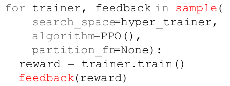
With a search space, a search algorithm, and an optional search space partition function, a search flow can be expressed as a for-loop, illustrated in Figure 10-left. Search space partitioning enables various ways in optimizing the divided sub-spaces, resulting in three basic search types: 1) optimize the sub-spaces jointly; 2) optimize the sub-spaces separately; or 3) factorize the optimization. Figure 10-right maps the three search types into different compositions of for-loop.
| Search type | for-loop pattern |
| Joint | |
| Separate | |
| Factorized | |
Let’s take the search space defined in Figure 9 as an example, which has a hyper-parameter sub-space (the hyper optimizer) and an architectural sub-space (the hyper model). Towards the two sub-spaces, we can 1) jointly optimize them without specifying a partition function, as is shown in Figure 10-left; 2) separately optimize them, by searching the hyper optimizer first with a fixed model, then use the best optimizer found to optimize the hyper model; or 3) factorize the optimization, by searching the hyper optimizer with a partition function in the outer loop. Each example in the loop is a trainer with a fixed optimizer and a hyper model; the latter will be optimized in the inner loop. The combination of these basic patterns can express very complex search flows, which will be further studied through our NAS-Bench-101 experiments discussed in Section 4.3.
3.5 Switching between search spaces
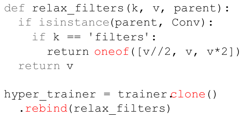
Making changes to the search space is a daily routine for AutoML practitioners, who may move from one search space to another, or to combine orthogonal search spaces into more complex ones. For example, we may start by searching for different operations at each layer, then try the idea of searching for different output filters (Figure 11), and eventually end up with searching for both. We showcase such search space exploration in Section 4.2.
3.6 Switching between search algorithms
The search algorithm is another dimension to experiment with. We can easily switch between search algorithms by passing a different algorithm to the sample function shown in Figure 10-1. When applying efficient NAS algorithms, the hyper_trainer will be rewritten into a trainer that samples and trains the super-network transformed from the architectural search space.
4 Case Study

In this section, we demonstrate that with PyGlove how users can define complex search spaces, explore new search spaces, search algorithms, and search flows with simplicity.
4.1 Expressing complex search spaces
The composition of hyper values can represent complex search spaces. We have reproduced popular NAS papers, including NAS-Bench-101 [38], MNASNet [8], NAS-FPN [39], ProxylessNAS [14], TuNAS [15], and NATS-Bench [40]. Here we use the search spaces from NAS-Bench-101, NAS-FPN, and TuNAS to demonstrate the expressiveness of PyGlove.
In the NAS-Bench-101 search space (Figure 12-top), there are different positions in the network and edge positions that can be independently turned on or off. Each node independently selects one of possible operations.
The NAS-FPN search space is a repeated FPN cell, each of whose nodes (Figure 12-middle) aggregates two outputs of previous nodes. The aggregation is either sum or global attention. We use manyof with the constraints distinct and sorted to select input nodes without duplication.
The TuNAS search space is a stack of blocks, each containing a number of residual layers (Figure 12-bottom) of inverted bottleneck units, whose filter size, kernel size and expansion factor will be tuned. To search the number of layers in a block, we put Zeros as a candidate in the Residual layer so the residual layer may downgrade into an identity mapping.
4.2 Exploring search spaces and search algorithms
We use MobileNetV2 [41] as an example to demonstrate how to explore new search spaces and search algorithms. For a fair comparison, we first retrain the MobileNetV2 model on ImageNet to obtain a baseline. With our training setup, it achieves a validation accuracy of 73.1% (Table 3, row 1) compared with 72.0% in the original MobileNetV2 paper. Details about our experiment setup, search space definitions, and the code for creating search spaces can be found in Appendix C.1.
Search space exploration: Similar to previous AutoML works [14, 8], we explore 3 search spaces derived from MobileNetV2 that tune the hyper-parameters of the inverted bottleneck units [41]: (1) Search space tunes the kernel size and expansion ratio. (2) Search space tunes the output filters (3) Search space combines and to tune the kernel size, expansion ratio and output filters.
From Table 3, we can see that with PyGlove we were able to convert MobileNetV2 into with 23 lines of code (row 2) and with 10 lines of code (row 5). From and , we obtain in just a single line of code (row 6) using rebind with chaining the transform functions from and .
Search algorithm exploration: On the search algorithm dimension, we start by exploring different search algorithms on using black-box search algorithms (Random Search [12], Bayesian [26]) and then efficient NAS (TuNAS [15]). To make model sizes comparable, we constrain the search to 300M multiply-adds222For RS and Bayesian, we use rejection sampling to ensure sampled architectures have around 300M MAdds. using TuNAS’s absolute reward function [15]. To switch between these algorithms, we only had to change 1 line of code.
| # | Search space | Search algorithm | Lines of codes | Search cost | Train cost | Test accuracy | # of MAdds | |
| 1 | () | N/A | N/A | N/A | 1 | 73.1 0.1 | 300M | |
| 2 | () | RS | +23 | 25 | 1 | 73.7 0.3 ( 0.6) | 300 3 M | |
| 3 | RS Bayesian | +1 | 25 | 1 | 73.9 0.3 ( 0.8) | 301 5 M | ||
| 4 | Bayesian TuNAS | +1 | 1 | 1 | 74.2 0.1 ( 1.1) | 301 5 M | ||
| 5 | TuNAS | +10 | 1 | 1 | 73.3 0.1 ( 0.2) | 302 7M | ||
| 6 | TuNAS | +1 | 2 | 1 | 73.8 0.1 ( 0.7) | 302 6M |
4.3 Exploring complex search flows on NAS-Bench-101
PyGlove can greatly reduce the engineering cost when exploring complex search flows. In this section, we explore various ways to optimize the NAS-Bench-101 search space. NAS-Bench-101 is a NAS benchmark where the goal is to find high-performing image classifiers in a search space of neural network architectures. This search space requires optimizing both the types of neural network layers used in the model (e.g., 3x3 Conv) and how the layers are connected.
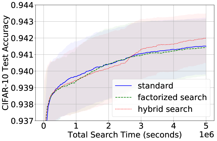
We experiment with three search flows in this exploration: 1) we reproduce the original paper to establish a baseline, which uses the search space defined in Figure 12-top to jointly optimize the nodes and edges. 2) we try a factorized search, which optimizes the nodes in the outer loop and the edges in the inner loop – the reward for a node setting is computed as the average of top 5 rewards from the architectures sampled in the inner loop. While its performance is not as good as the baseline under the same search budget, we suspect that under each fixed node setting, the edge space is not explored enough. 3) To alleviate this problem, we come out a hybrid solution, which uses the first half of the budget to optimize the nodes as in search flow 2, while using the other half to optimize the edges, based on the best node setting found in the first phase. Interestingly, the search trajectory crosses over the baseline in the second phase, ended with a noticeable margin (Figure 13). We used Regularized Evolution [16] for all these searches, each with 500 runs. It takes only 15 lines of code to implement the factorized search and 26 lines of code to implement the hybrid search. Source codes are included in Appendix C.2.
5 Related Work
Software frameworks
have greatly influenced and fueled the advancement of machine learning. The need for computing gradients has made auto-gradient based frameworks [42, 37, 36, 43, 44, 45] flourish. To support modular machine learning programs with the flexibility to modify them, frameworks were introduced with an emphasis on hyper-parameter management [46, 47]. The sensitivity of machine learning to hyper-parameters and model architecture has led to the advent of AutoML libraries [23, 24, 25, 26, 27, 28, 29, 30, 31]. Some (e.g., [23, 24, 25]) formulate AutoML as a problem of jointly optimizing architectures and hyper-parameters. Others (e.g., [26, 27, 28]) focus on providing interfaces for black-box optimization. In particular, Google’s Vizier library [26] provides tools for optimizing a user-specified search space using black-box algorithms [12, 48], but makes the end user responsible for translating a point in the search space into a user program. DeepArchitect [29] proposes a language to create a search space as a program that connects user components. Keras-tuner [30] employs a different way to annotate a model into a search space, though this annotation is limited to a list of supported components. Optuna [49] embraces eager evaluation of tunable parameters, making it easy to declare a search space on the go (Appendix B.4). Meanwhile, efficient NAS algorithms [1, 2, 14] brought new challenges to AutoML frameworks, which require coupling between the controller and child program. AutoGluon [28] and NNI [27] partially solve this problem by building predefined modules that work in both general search mode and weight-sharing mode, however, supporting different efficient NAS algorithms are still non-trivial. Among the existing AutoML systems we are aware of, complex search flows are less explored. Compared to existing systems, PyGlove employs a mutable programming model to solve these problems, making AutoML easily accessible to preexisting ML programs. It also accommodates the dynamic interactions among the child programs, search spaces, search algorithms, and search flows to provide the flexibility needed for future AutoML research.
Symbolic programming
, where a program manipulates symbolic representations, has a long history dating back to LISP [20]. The symbolic representation can be programs as in meta-programming, rules as in logic programming [50] and math expressions as in symbolic computation [51, 52]. In this work, we introduce the symbolic programming paradigm to AutoML by manipulating a symbolic tree-based representation that encodes the key elements of a machine learning program. Such program manipulation is also reminiscent of program synthesis [53, 54, 55], which searches for programs to solve different tasks like string and number manipulation [56, 57, 58, 59], question answering [60, 61], and learning tasks [62, 63]. Our method also shares similarities with prior works in non-deterministic programming [64, 65, 66], which define non-deterministic operators like choice in the programming environment that can be connected to optimization algorithms. Last but not least, our work echos the idea of building robust software systems that can cope with unanticipated requirements via advanced symbolic programming [67].
6 Conclusion
In this paper, we reformulate AutoML as an automated process of manipulating a ML program through symbolic programming. Under this formulation, the complex interactions between the child program, the search space, and the search algorithm are elegantly disentangled. Complex search flows can be expressed as compositions of for-loops, greatly simplifying the programming interface of AutoML without sacrificing flexibility. This is achieved by resolving the conflict between AutoML’s intrinsic requirement in modifying programs and the immutable-program premise of existing software libraries. We then introduce PyGlove, a general-purpose symbolic programming library for Python which implements our method and is tested on real-world AutoML scenarios. With PyGlove, AutoML can be easily dropped into preexisting ML programs, with all program parts searchable, permitting rapid exploration of different dimensions of AutoML.
Broader Impact
Symbolic programming/PyGlove makes AutoML more accessible to machine learning practitioners, which means manual trial-and-error of many categories can be replaced by machines. This can also greatly increase the productivity of AutoML research, at the cost of increasing demand for computation, and – a result – increasing emissions.
We see a big potential in symbolic programming/PyGlove in making machine learning researchers more productive. On a new ground of mutable programs, experiments can be reproduced more easily, modified with lower cost, and shared like data. A large variety of experiments can co-exist in a shared code base that makes combining and comparing different techniques more convenient.
Symbolic programming/PyGlove makes it much easier to develop search-based programs which can be used in a broad spectrum of research and product areas. Some potential areas, such as medicine design, have a clear societal benefit, while others potential applications, such as video surveillance, could improve security while raising new privacy concerns.
Acknowledgments and Disclosure of Funding
We would like to thank Pieter-Jan Kindermans and David Dohan for their help in preparing the case study section of this paper; Jiquan Ngiam, Rishabh Singh for their feedback to the early versions of the paper; Ruoming Pang, Vijay Vasudevan, Da Huang, Ming Cheng, Yanping Huang, Jie Yang, Jinsong Mu for their feedback at early stage of PyGlove; Adams Yu, Daniel Park, Golnaz Ghiasi, Azade Nazi, Thang Luong, Barret Zoph, David So, Daniel De Freitas Adiwardana, Junyang Shen, Lav Rai, Guanhang Wu, Vishy Tirumalashetty, Pengchong Jin, Xianzhi Du, Yeqing Li, Xiaodan Song, Abhanshu Sharma, Cong Li, Mei Chen, Aleksandra Faust, Yingjie Miao, JD Co-Reyes, Kevin Wu, Yanqi Zhang, Berkin Akin, Amir Yazdanbakhsh, Shuyang Cheng, HyoukJoong Lee, Peisheng Li and Barbara Wang for being early adopters of PyGlove and their invaluable feedback.
Funding disclosure: This work was done as a part of the authors’ full-time job in Google.
References
- [1] Hieu Pham, Melody Y Guan, Barret Zoph, Quoc V Le, and Jeff Dean. Efficient neural architecture search via parameter sharing. In The International Conference on Machine Learning (ICML), pages 4092–4101, 2018.
- [2] Hanxiao Liu, Karen Simonyan, and Yiming Yang. DARTS: Differentiable architecture search. In International Conference on Learning Representations (ICLR), 2019.
- [3] Gábor Melis, Chris Dyer, and Phil Blunsom. On the state of the art of evaluation in neural language models. In International Conference on Learning Representations (ICLR), 2018.
- [4] Alfredo Canziani, Adam Paszke, and Eugenio Culurciello. An analysis of deep neural network models for practical applications. arXiv preprint arXiv:1605.07678, 2016.
- [5] Alex Krizhevsky, Ilya Sutskever, and Geoffrey E Hinton. Imagenet classification with deep convolutional neural networks. In The Conference on Neural Information Processing Systems (NeurIPS), pages 1097–1105, 2012.
- [6] Mingxing Tan and Quoc Le. EfficientNet: Rethinking model scaling for convolutional neural networks. In The International Conference on Machine Learning (ICML), pages 6105–6114, 2019.
- [7] Barret Zoph, Vijay Vasudevan, Jonathon Shlens, and Quoc V Le. Learning transferable architectures for scalable image recognition. In Proceedings of the IEEE Conference on Computer Vision and Pattern Recognition (CVPR), pages 8697–8710, 2018.
- [8] Mingxing Tan, Bo Chen, Ruoming Pang, Vijay Vasudevan, Mark Sandler, Andrew Howard, and Quoc V Le. MNASNet: Platform-aware neural architecture search for mobile. In Proceedings of the IEEE Conference on Computer Vision and Pattern Recognition (CVPR), pages 2820–2828, 2019.
- [9] Barret Zoph and Quoc V Le. Neural architecture search with reinforcement learning. In International Conference on Learning Representations (ICLR), 2017.
- [10] Bichen Wu, Xiaoliang Dai, Peizhao Zhang, Yanghan Wang, Fei Sun, Yiming Wu, Yuandong Tian, Peter Vajda, Yangqing Jia, and Kurt Keutzer. FbNet: Hardware-aware efficient convnet design via differentiable neural architecture search. In Proceedings of the IEEE Conference on Computer Vision and Pattern Recognition (CVPR), pages 10734–10742, 2019.
- [11] Xiaoliang Dai, Peizhao Zhang, Bichen Wu, Hongxu Yin, Fei Sun, Yanghan Wang, Marat Dukhan, Yunqing Hu, Yiming Wu, Yangqing Jia, et al. ChamNet: Towards efficient network design through platform-aware model adaptation. In Proceedings of the IEEE Conference on Computer Vision and Pattern Recognition, pages 11398–11407, 2019.
- [12] James Bergstra and Yoshua Bengio. Random search for hyper-parameter optimization. The Journal of Machine Learning Research (JMLR), 13(Feb):281–305, 2012.
- [13] Jasper Snoek, Hugo Larochelle, and Ryan P Adams. Practical bayesian optimization of machine learning algorithms. In The Conference on Neural Information Processing Systems (NeurIPS), pages 2951–2959, 2012.
- [14] Han Cai, Ligeng Zhu, and Song Han. ProxylessNAS: Direct neural architecture search on target task and hardware. In International Conference on Learning Representations (ICLR), 2019.
- [15] Gabriel Bender, Hanxiao Liu, Bo Chen, Grace Chu, Shuyang Cheng, Pieter-Jan Kindermans, and Quoc Le. Can weight sharing outperform random architecture search? an investigation with TuNAS. In The IEEE Conference on Computer Vision and Pattern Recognition, 2020.
- [16] Esteban Real, Alok Aggarwal, Yanping Huang, and Quoc V Le. Regularized evolution for image classifier architecture search. In AAAI Conference on Artificial Intelligence (AAAI), pages 4780–4789, 2019.
- [17] Sirui Xie, Hehui Zheng, Chunxiao Liu, and Liang Lin. Snas: Stochastic neural architecture search, 2020.
- [18] Wei Wen, Hanxiao Liu, Hai Li, Yiran Chen, Gabriel Bender, and Pieter-Jan Kindermans. Neural predictor for neural architecture search. In Proceedings of the European Conference on Computer Vision (ECCV), 2020.
- [19] Xuanyi Dong, Mingxing Tan, Adams Wei Yu, Daiyi Peng, Bogdan Gabrys, and Quoc V Le. AutoHAS: Efficient hyperparameter and architecture search. arXiv preprint arXiv:2006.03656, 2020.
- [20] John McCarthy. Recursive functions of symbolic expressions and their computation by machine, part i. Communications of the ACM, 3(4):184–195, 1960.
- [21] Symbolic programming. https://en.wikipedia.org/wiki/Symbolic_programming.
- [22] Esteban Real, Sherry Moore, Andrew Selle, Saurabh Saxena, Yutaka Leon Suematsu, Jie Tan, Quoc V Le, and Alexey Kurakin. Large-scale evolution of image classifiers. In The International Conference on Machine Learning (ICML), pages 2902–2911, 2017.
- [23] Matthias Feurer, Aaron Klein, Katharina Eggensperger, Jost Springenberg, Manuel Blum, and Frank Hutter. Efficient and robust automated machine learning. In The Conference on Neural Information Processing Systems (NeurIPS), pages 2962–2970, 2015.
- [24] Lars Kotthoff, Chris Thornton, Holger H Hoos, Frank Hutter, and Kevin Leyton-Brown. Auto-weka 2.0: Automatic model selection and hyperparameter optimization in weka. The Journal of Machine Learning Research (JMLR), 18(1):826–830, 2017.
- [25] Matthias Feurer, Aaron Klein, Katharina Eggensperger, Jost Tobias Springenberg, Manuel Blum, and Frank Hutter. Auto-sklearn: efficient and robust automated machine learning. In Automated Machine Learning, pages 113–134. Springer, 2019.
- [26] Daniel Golovin, Benjamin Solnik, Subhodeep Moitra, Greg Kochanski, John Karro, and D Sculley. Google vizier: A service for black-box optimization. In The SIGKDD International Conference on Knowledge Discovery and Data Mining, pages 1487–1495, 2017.
- [27] Neural network intelligence. https://github.com/microsoft/nni.
- [28] Nick Erickson, Jonas Mueller, Alexander Shirkov, Hang Zhang, Pedro Larroy, Mu Li, and Alexander Smola. Autogluon-tabular: Robust and accurate automl for structured data. arXiv preprint arXiv:2003.06505, 2020.
- [29] Renato Negrinho, Darshan Patil, Nghia Le, Daniel Ferreira, Matthew Gormley, and Geoffrey Gordon. Towards modular and programmable architecture search. In The Conference on Neural Information Processing Systems (NeurIPS), pages 13715–13725, 2019.
- [30] Keras tuner. https://github.com/keras-team/keras-tuner.
- [31] Haifeng Jin, Qingquan Song, and Xia Hu. Auto-keras: An efficient neural architecture search system. In The SIGKDD International Conference on Knowledge Discovery and Data Mining, pages 1946–1956, 2019.
- [32] The Lego Group. Lego. https://en.wikipedia.org/wiki/Lego.
- [33] Ronald J Williams. Simple statistical gradient-following algorithms for connectionist reinforcement learning. Machine learning, 8(3-4):229–256, 1992.
- [34] Jeshua Bratman, Satinder Singh, Jonathan Sorg, and Richard Lewis. Strong mitigation: Nesting search for good policies within search for good reward. In Proceedings of the 11th International Conference on Autonomous Agents and Multiagent Systems-Volume 1, pages 407–414. International Foundation for Autonomous Agents and Multiagent Systems, 2012.
- [35] Arber Zela, Aaron Klein, Stefan Falkner, and Frank Hutter. Towards automated deep learning: Efficient joint neural architecture and hyperparameter search. CoRR, abs/1807.06906, 2018.
- [36] Adam Paszke, Sam Gross, Francisco Massa, Adam Lerer, James Bradbury, Gregory Chanan, Trevor Killeen, Zeming Lin, Natalia Gimelshein, Luca Antiga, et al. PyTorch: An imperative style, high-performance deep learning library. In The Conference on Neural Information Processing Systems (NeurIPS), pages 8024–8035, 2019.
- [37] Martín Abadi, Paul Barham, Jianmin Chen, Zhifeng Chen, Andy Davis, Jeffrey Dean, Matthieu Devin, Sanjay Ghemawat, Geoffrey Irving, Michael Isard, et al. Tensorflow: A system for large-scale machine learning. In The USENIX Symposium on Operating Systems Design and Implementation (OSDI 16), pages 265–283, 2016.
- [38] Chris Ying, Aaron Klein, Eric Christiansen, Esteban Real, Kevin Murphy, and Frank Hutter. Nas-bench-101: Towards reproducible neural architecture search. In The International Conference on Machine Learning (ICML), pages 7105–7114, 2019.
- [39] Golnaz Ghiasi, Tsung-Yi Lin, Ruoming Pang, and Quoc V. Le. NAS-FPN: learning scalable feature pyramid architecture for object detection. CoRR, abs/1904.07392, 2019.
- [40] Xuanyi Dong, Lu Liu, Katarzyna Musial, and Bogdan Gabrys. NATS-Bench: Benchmarking nas algorithms for architecture topology and size. arXiv preprint arXiv:2009.00437, 2020.
- [41] Mark Sandler, Andrew Howard, Menglong Zhu, Andrey Zhmoginov, and Liang-Chieh Chen. Mobilenetv2: Inverted residuals and linear bottlenecks. In Proceedings of the IEEE conference on computer vision and pattern recognition, pages 4510–4520, 2018.
- [42] James Bergstra, Olivier Breuleux, Frédéric Bastien, Pascal Lamblin, Razvan Pascanu, Guillaume Desjardins, Joseph Turian, David Warde-Farley, and Yoshua Bengio. Theano: a cpu and gpu math expression compiler. In Proceedings of the Python for scientific computing conference (SciPy), pages 18–24, 2010.
- [43] Yangqing Jia, Evan Shelhamer, Jeff Donahue, Sergey Karayev, Jonathan Long, Ross Girshick, Sergio Guadarrama, and Trevor Darrell. Caffe: Convolutional architecture for fast feature embedding. In The ACM International Conference on Multimedia (ACM MM), pages 675–678, 2014.
- [44] Seiya Tokui. Chainer: A powerful, flexible and intuitive framework of neural networks, 2018.
- [45] Roy Frostig, Matthew Johnson, and Chris Leary. Compiling machine learning programs via high-level tracing. In Conference on Machine Learning and Systems (MLSys), 2018.
- [46] Jonathan Shen, Patrick Nguyen, Yonghui Wu, Zhifeng Chen, Mia X Chen, Ye Jia, Anjuli Kannan, Tara Sainath, Yuan Cao, Chung-Cheng Chiu, et al. Lingvo: a modular and scalable framework for sequence-to-sequence modeling. arXiv preprint arXiv:1902.08295, 2019.
- [47] Gin-config. https://github.com/google/gin-config.
- [48] Max Jaderberg, Valentin Dalibard, Simon Osindero, Wojciech M Czarnecki, Jeff Donahue, Ali Razavi, Oriol Vinyals, Tim Green, Iain Dunning, Karen Simonyan, et al. Population based training of neural networks. arXiv preprint arXiv:1711.09846, 2017.
- [49] Takuya Akiba, Shotaro Sano, Toshihiko Yanase, Takeru Ohta, and Masanori Koyama. Optuna: A next-generation hyperparameter optimization framework. In Proceedings of the 25rd ACM SIGKDD International Conference on Knowledge Discovery and Data Mining, 2019.
- [50] Alain Colmerauer and Philippe Roussel. The birth of prolog. In History of programming languages—II, pages 331–367, 1996.
- [51] Wolfram Research, Inc. Mathematica, Version 12.1. Champaign, IL, 2020.
- [52] Bruno Buchberger et al. Symbolic computation (an editorial). J. Symbolic Comput, 1(1):1–6, 1985.
- [53] Harold Abelson and Gerald Jay Sussman. Structure and interpretation of computer programs. The MIT Press, 1996.
- [54] Sumit Gulwani, Susmit Jha, Ashish Tiwari, and Ramarathnam Venkatesan. Synthesis of loop-free programs. ACM SIGPLAN Notices, 46(6):62–73, 2011.
- [55] Sumit Gulwani, Oleksandr Polozov, and Rishabh Singh. Program synthesis. Foundations and Trends® in Programming Languages, 4(1-2):1–119, 2017.
- [56] Oleksandr Polozov and Sumit Gulwani. Flashmeta: a framework for inductive program synthesis. In Proceedings of the ACM SIGPLAN International Conference on Object-Oriented Programming, Systems, Languages, and Applications (OOPSLA), pages 107–126, 2015.
- [57] Emilio Parisotto, Abdel rahman Mohamed, Rishabh Singh, Lihong Li, Dengyong Zhou, and Pushmeet Kohli. Neuro-symbolic program synthesis. In International Conference on Learning Representations (ICLR), 2017.
- [58] Jacob Devlin, Jonathan Uesato, Surya Bhupatiraju, Rishabh Singh, Abdel rahman Mohamed, and Pushmeet Kohli. Robustfill: Neural program learning under noisy i/o. In The International Conference on Machine Learning (ICML), pages 990–998, 2017.
- [59] Matej Balog, Alexander L Gaunt, Marc Brockschmidt, Sebastian Nowozin, and Daniel Tarlow. DeepCoder: Learning to write programs. In International Conference on Learning Representations (ICLR), 2017.
- [60] Chen Liang, Mohammad Norouzi, Jonathan Berant, Quoc V. Le, and Ni Lao. Memory augmented policy optimization for program synthesis and semantic parsing. In The Conference on Neural Information Processing Systems (NeurIPS), pages 9994–10006, 2018.
- [61] Arvind Neelakantan, Quoc V. Le, and Ilya Sutskever. Neural programmer: Inducing latent programs with gradient descent. In International Conference on Learning Representations (ICLR), 2016.
- [62] Esteban Real, Chen Liang, David R So, and Quoc V Le. Automl-zero: Evolving machine learning algorithms from scratch. In The International Conference on Machine Learning (ICML), 2020.
- [63] Lazar Valkov, Dipak Chaudhari, Akash Srivastava, Charles Sutton, and Swarat Chaudhuri. Houdini: Lifelong learning as program synthesis. In The Conference on Neural Information Processing Systems (NeurIPS), pages 8687–8698, 2018.
- [64] D. Andre and S. Russell. State abstraction in programmable reinforcement learning. In AAAI Conference on Artificial Intelligence (AAAI), 2002.
- [65] Harald Søndergaard and Peter Sestoft. Non-determinism in functional languages. The Computer Journal, 35(5):514–523, 1992.
- [66] Armando Solar-Lezama. The sketching approach to program synthesis. In Asian Symposium on Programming Languages and Systems, pages 4–13. Springer, 2009.
- [67] G. Sussman. Building robust systems an essay. In Massachusetts Institute of Technology, 2007.
Appendix
The appendix provides a formal definition of symbolic programs in our method, including symbolic counterparts of different program constructs, supported operations, and the description of algorithms used in the materialization process. Appendix B gives a more detailed introduction to PyGlove – our implementation of the method – with an example of dropping neural architecture search (NAS) into an existing Tensorflow program (MNIST [37]). Appendix C provides additional information for experiments used in our case studies, including experiment setup, source code for creating search spaces and complex search flows.
Appendix A More on Symbolic Programming for AutoML
A.1 Formal definition of a symbolic program
Give a program construct type , let the hyper-parameters (which defines the uniqueness of an instance of ) be noted as . The symbolic type of can then be defined as the output of the symbolization function applied on , which returns a tuple of ’s type information and its hyper-parameter definitions:
| (1) |
A hyper-parameter of is either a primitive type or a symbolic type. Therefore an instance of – a symbolic object – is a tree node, whose sub-nodes are its hyper-parameters. For convenience, is called a symbolic , e.g: symbolic Dataset, symbolic Conv, etc. A symbolic program is a symbolic object that can be executed, for example, a symbolic Trainer that trains and evaluates a ResNet (as a sub-node) on ImageNet.
Two tree nodes are equal if and only if their type and hyper-parameters are equal. For example, consider a symbolic Conv class which takes filters, kernel_size as its hyper-parameters. Two Conv instances are equal if and only if their filters and kernel_size are equal.
We can clone a tree by copying its type information and hyper-parameters. Similarly, we can replace a hyper-parameter value with a new value, which is the foundation for symbolic manipulation. For example, a symbolic Conv’s kernel_size can be changed from to by another program.
Symbolic constraints can be specified on the hyper-parameters. These constraints define the hyper-parameters’ value types and ranges. When a value is assigned as a hyper-parameter of another symbolic object, it will be validated based on the symbolic constraint on that hyper-parameter. Since the sub-nodes of a symbolic object can be manipulated, the constraints are helpful in catching mistakes during symbolic manipulation.
A.2 Symbolic types
The basic elements of a computer program are classes and functions, plus a few built-in data structure that works with the classes and functions for composition. To symbolize a computer program, we need to map these basic program constructs to their symbolic counterparts. Based on Equation 1, the symbolic type of is defined by ’s type information and hyper-parameters, illustrated in Table 4
| Program construct type | Hyper-parameters |
| class | Constructor arguments. |
| function | Function arguments. |
| list | Indices in the list. |
| dict | Keys in the dict. |
Though a regular function takes arguments, the function itself doesn’t hold its hyper-parameter values. Therefore, in order to manipulate the hyper-parameters of a function, a symbolic function – functor – behaves like an object: an function with bound arguments. As a result, a functor is no different from a class object with a call method, whose arguments could be bound either at construction time or call time. Therefore, a functor can be a node in the symbolic tree.
A.3 Operations on symbolic types
Symbolic objects can be manipulated via a set of operations. Table 5 lists the basic operations applicable to all symbolic types. Particularly, rebind in the modification category is of special importance, as it’s the foundation for implementing complex program transforms.
| Category | Operation | Description | ||
| Modification | rebind() | Replace each node in whose path is a key in dict | ||
| rebind() | Recursively apply the function to each node in | |||
| Inference | isinstance(, ) | Returns true if is an instance of , false otherwise | ||
| has(, ) | Returns true if is a property of , false otherwise | |||
| equal(, ) | Returns true if equals , false otherwise | |||
| Inquiry | parent() | Returns the parent node of | ||
| path() | Returns the path from the tree root to | |||
| get(, ) | Returns the sub-node of which has path | |||
| query(, ) |
|
|||
| Replication | clone() | Returns a symbolic copy of |
A.4 Materializing a child program from an abstract child program
As we decouple the search algorithm from the search space and child program by introducing the abstract search space and abstract child program, we need to materialize the abstract child program into a concrete child program based on the search space. Algorithm 1 illustrates this process, which recursively merges the hyper values from the search space and the numeric choices from the abstract child program. For a continuous or discrete hyper value, the value of choice is the final value to be assigned to its target node in the tree, while for a categorical hyper value, the value of choice is the index of the selected candidate.
A.5 Sampling child programs from a search space
Sampling a child program from a search space can be described as a process in which 1) the search algorithm proposes an abstract child program, and 2) the search space materializes the abstract child program into a concrete program. Before the process starts, an abstract search space will be obtained from the search space for setting up the search algorithm. This process is described by Algorithm 2.
Appendix B More on PyGlove
In this section, we will map the concepts from our method into PyGlove programs, to illustrate how a regular Python program is made symbolic programmable, turned into a search space, and then optimized in a search flow. At the end of this section, we provide an example of enabling NAS for an existing Tensorflow-based MNIST program.
B.1 Symbolize a child program
B.1.1 Symbolize classes
A symbolic class can be converted from a regular Python class using the @symbolize decorator, or can be created on-the-fly without modifying the original class. The symbolize decorator creates a class on-the-fly by multi-inheriting the symbolic Object base class and the user class. The resulting class therefore possesses the capabilities of both parents. Figure 14 shows an code example of symbolizing existing/new classes.
Using symbolic constraints
Constraints which validate new values during object construction or upon modification can be optionally provided when using the @symbolize decorator. Symbolic constraints can greatly reduce human mistakes when a program is manipulated by other programs. It also make the program implementation more crisp: user can program against an argument as it claims to be without additional check.
Recomputing internal states
Symbolic objects may have internal states. The mutable programming model will only work when the internal states are consistent upon modification. When one or more hyper-parameters are modified through rebind, the object’s state will be reset, and the object’s constructor will be invoked (again) on the same instance. Moreover, the change propagates back from the current node to the root of the symbolic tree, allowing all impacted nodes to recompute states upon modification.
B.1.2 Symbolize functions
From function to functor
Making functions symbolic programmable is trickier than for classes, for the following reasons: First: functions don’t explicitly hold their parameters as member variables, although functions’ bound arguments are analogous to member variables in classes. Second: functions don’t have the concept of inheritance, which is necessary to get access to the capabilities provided by the symbolic Object base class. To address these two issues, we introduce the concept of functor, which is a symbolic class with a __call__ method; all the function arguments becoming the functor’s hyper-parameters. Under the functor concept, we unify the representation and operations of classes and functions. Figure 15 shows that functions can be symbolized in the same way as we symbolize classes. Figure 16 shows how functors can be used with great flexibility in binding their hyper-parameters.
Partial and incremental argument binding
Functor comes with a capability that allows arguments to be partially bound at construction time, incrementally bound via property assignment and at call time. We can even override a previously bound argument during the call to the functor.
B.2 Operating symbolic values
Symbolic values can be operated as if they were plain data, including inference, inquiry, modification and replication. Figure 17 gives some examples to these operations.
B.3 Using PyGlove for search
B.3.1 Creating search spaces
With the definition of functors train_model and random_augment, as well as the layer classes, we can create a search space by replacing concrete values with hyper values, illustrated in Figure 18.
B.3.2 Search: putting things together
With hyper_trainer as the search space, we can start a search by sampling concrete trainers from the search space with a search algorithm (e.g. RegularizedEvolution [16]). The trainer is a concrete instance of train_model, which can be invoked to return the validation accuracy on ImageNet. We use the validation accuracy as a reward to feedback to the search algorithm, illustrated in Figure 19.
B.4 More on materialization of hyper values
Materialization of hyper values can take place either eagerly or in a late-bound fashion. In the former case, the hyper value evaluates to a concrete value within its range upon creation, and register the search space into a global context for the first run, which can be picked up by the search algorithm later to propose values for future runs. This conditional evaluation makes it possible to support the define-by-run style search space definition advocated by Optuna [49]. In the latter case, the search space will be inspected from the symbolic tree and the tree can be manipulated freely by the search algorithm before the program is executed.
The advantage of eager evaluation is that one can drop AutoML into a new ML program with minimal code changes. Users do not need to explicitly define the hyper-parameters to search. Instead, we can automatically identify them by executing the user’s code before the start of the search. On the other hand, scattered searchable hyper-parameters makes it hard or error-prone to modify search space over many files, especially when we want to explore multiple search spaces.
Meanwhile, conditional search spaces require special handling. Define-by-run semantics typically do not provide enough information for us to recognize hierarchical search spaces. For instance, it is difficult to distinguish between oneof([oneof([1, 2]), 1]) and oneof([1, 2]) + oneof([3, 4]). In PyGlove, we solve this problem by using a lambda function with zero-argument which returns the candidate: oneof([lambda:oneof([1, 2]), 1]). In this case, the outer oneof will instantiate the inner oneof, making it possible to capture the hierarchy of the hyper value structure.
While eagerly evaluation of hyper values seems to override the mechanism of symbolic manipulation, it is not so for PyGlove: Under eager mode, PyGlove runs the user program once to collect the symbolic objects (like the hyper values) along the program flow, so we can access these objects, manipulate them and inject them back into the program for future runs. As a result, eagerly evaluation can be regarded as an interface for PyGlove to inspect and manipulate the implicit symbolic objects created during program execution.
B.5 Example: Neural Architecture Search on MNIST
This section shows a complete example of dropping PyGlove into an existing ML program as to enable NAS. Added code is highlighted with a light-yellow background.
Appendix C More on case studies
This section describes the experiment details for our case studies in the paper.
C.1 Search spaces and search algorithms exploration
C.1.1 Experiment setup
| Name | Value |
| Image size | 224 * 224 |
| Pre-processing | ResNet preprocessing |
| Training epochs | 360 |
| Batch size | 4096 |
| Optimizer | RMSProp: momentum 0.9, decay 0.9, epsilon 1.0 |
| Learning schedule | Cosine decay with peak learning rate 2.64, with 5 epochs linear warmup at the beginning. |
| L2 | 2e-5 |
| Dropout rate | 0.15 |
| Batch normalization | momentum 0.99, epsilon 0.001 |
| Search space | Hyper-parameters |
| Search the kernel sizes with candidates [(3, 3), (5, 5), (7, 7)] | |
| and expansion ratios with candidates [3, 6] for the inverted bottleneck units | |
| in MobileNetV2; can remove layers from each block. | |
| Search output filters of MobileNetV2 | |
| with multipliers [0.5, 0.625, 0.75, 1.0, 1.25, 1.5, 2.0] | |
| Combine and |
| Search algorithm | Configuration |
| Random Search [12] | 100 trials, each trial trains for 90 epochs, |
| rejection threshold for MAdds: 6M | |
| Bayesian Optimization [26] | 100 trials, each trial trains for 90 epochs |
| rejection threshold for MAdds: 30M | |
| (We use a larger rejection ratio for Bayesian | |
| to limit the rejection rate, since our infra | |
| will take the rewards from rejected trials) | |
| TuNAS [15] | Search for 90 epochs, with RL learning rate set to 0 for first 1/4 of training. The search cost for and is about 4x of static model training, and the cost for about 8x of static model training. |
C.1.2 Creating search spaces
In the Result section, we demonstrated 3 search spaces created from MobileNetV2 [41]. Figure 21-23 show the code for converting the static model into search spaces , and .
C.2 Search flow exploration
In the case study, we explored 3 search flows for optimizing NAS-Bench-101. Here we include the code for the factorized and hybrid search since the standard search is already discussed in Section B.3.2.
C.2.1 Factorized search
For the factorized search, we optimize the nodes in the outer loop and the edges in the inner loop. Each example in the outer loop is a search space of edges with a fixed node setting. Each example in the inner loop is a fixed model architecture. The reward for the outer loop is computed as the average of top 5 rewards from the inner loop.
C.2.2 Hybrid search
For the hybrid search, we use the first half of the budget to optimize the nodes using the same search flow illustrated in Section C.2.1 , then we use the other half of the budget to further optimize the edges with the best nodes found in the prior phase.